Kitaev-like honeycomb magnets: Global phase behavior and emergent effective models

Abstract

Compounds of transition metal ions with strong spin-orbit coupling recently attracted attention due to the possibility to host frustrated bond-dependent anisotropic magnetic interactions. In general, such interactions lead to complex phase diagrams that may include exotic phases, e.g. the Kitaev spin liquid. Here we report on our comprehensive analysis of the global phase diagram of the extended Kitaev-Heisenberg model relevant to honeycomb lattice compounds Na₂IrO₃ and $\alpha$-RuCl₃. We have utilized recently developed method based on spin coherent states that enabled us to resolve arbitrary spin patterns in the cluster ground states obtained by exact diagonalization. Global trends in the phase diagram are understood in combination with the analytical mappings of the Hamiltonian that uncover peculiar links to known models – Heisenberg, Ising, Kitaev, or compass models on the honeycomb lattice – or reveal entire manifolds of exact fluctuation-free ground states. Finally, our study can serve as a methodological example that can be applied to other spin models with complex bond-dependent non-Heisenberg interactions.

I Introduction

In contrast to simple examples of Heisenberg magnets discussed in standard textbooks, frustrated spin systems [1] offer much wider range of phenomena, including the exotic spin-liquid behavior [2; 3] or the emergence of effective monopoles in spin-ice pyrochlores [4; 5]. The usual sources of frustration are frustrated geometry of the lattice (e.g. kagomé [6]) or the presence of longer-range interactions competing with the nearest-neighbor ones (as e.g. in $J_{1}$-$J_{2}$ model [7; 8; 9]) and possibly among themselves. Within the last decade, pseudospin-$\frac{1}{2}$ systems with frustrated bond-dependent non-Heisenberg interactions emerging in Mott insulators as a consequence of spin-orbit coupling (SOC) became a subject of intense research [10; 11; 12; 13; 14; 15; 16]. While one of the main motivations has been a possible realization of the Kitaev honeycomb model [17], the presence of additional interactions leads to very rich magnetic behavior that is particularly attractive as well as challenging to study.

The basic element enabling the realization of the above models possessing bond-dependent anisotropic interactions has been well known for a long time. It relies on a $d^{5}$ valence configuration of heavy transition-metal ions with large SOC which combines the spin $s=\frac{1}{2}$ and effective orbital angular momentum $l_{\mathrm{eff}}=1$ of the hole in the $t_{2g}^{5}$ configuration into $J_{\mathrm{eff}}=\frac{1}{2}$ Kramers doublet ground state [18; 19]. A direct experimental evidence for the spin-orbital entangled multiplet structure [20] was obtained e.g. by resonant x-ray scattering on Sr₂IrO₄ [21] containing $d^{5}$ Ir⁴⁺ ions. It was the seminal theoretical proposal by Jackeli and Khaliullin [22] that suggested how to exploit the $J_{\mathrm{eff}}=\frac{1}{2}$ pseudospins in Mott insulators with large SOC. Two lines of intense research followed. The first one focuses on the square lattice case with the resulting Heisenberg interactions among the pseudospins – a situation appealingly analogous to undoped cuprates. Cuprate-like magnetism was indeed found in perovskite iridates [23] and certain observations support the idea to extend the analogy to the doped case [24; 25]. Yet bigger excitement was initiated by a proposal that the honeycomb $J_{\mathrm{eff}}=\frac{1}{2}$ compounds may be close to the Kitaev limit where Ising-like bond-dependent interactions lead to a spin-liquid ground state. Such an exotic effective spin system may naturally arise when translating the bond-anisotropic interactions of the $d$ orbitals appearing in Kugel-Khomskii models [26] into the pseudospin space via the SOC-induced spin-orbital entanglement [19; 27].

In the search of materials close to the Kitaev limit, much attention has been paid to the honeycomb iridates Na₂IrO₃, $\alpha$-Li₂IrO₃, and the ruthenate $\alpha$-RuCl₃ [28] that is claimed to show signatures of Kitaev physics in the excitation spectra [29; 30; 31; 32]. However, these compounds were found to host long-range magnetic order instead – zigzag type in Na₂IrO₃ [33; 34; 35] and $\alpha$-RuCl₃ [36; 37; 29] and spiral type in $\alpha$-Li₂IrO₃ [38]. Only very recently, an evidence for a liquid state was found in a related compound H₃LiIr₂O₆ [39]. Even though the zigzag phase is present in the phase diagram of the originally proposed Kitaev-Heisenberg model [40], later experiments on Na₂IrO₃ showed that it gives an inconsistent ordered moment direction [41] and additional bond-anisotropic and/or further-neighbor interactions have to be invoked [42; 43; 44; 45; 46; 47]. In the resulting extended Kitaev-Heisenberg models, the highly anisotropic interactions lead to complex phase behavior (see Refs. [42; 43; 15] for examples) or unusual spin excitation spectra showing e.g. a breakdown of the magnon picture even in the long-range ordered phase away from the Kitaev limit [48] or topological features [49; 50].

The (extended) Kitaev-Heisenberg models are not limited to the honeycomb lattice. A large number of other situations have been discussed, including triangular [19; 51; 52; 53; 54] and kagomé [55] lattice and suitable types of three-dimensional structures such as experimentally realized hyperhoneycomb [56; 57; 58; 59; 60], harmonic honeycomb [61; 62; 63; 57; 59], hyperkagomé [64; 27], fcc [65; 66; 67], and pyrochlore lattices [68; 69], or hypothetical hyperoctagon lattice [70]. Finally, the concept of Kitaev interactions in pseudospin $J_{\mathrm{eff}}=\frac{1}{2}$ systems has been recently extended to $d^{7}$ compounds such as those containing Co²⁺ [71; 72].

In general, a thorough inspection of an extended Kitaev-Heisenberg model in terms of spin structures, excitations etc. through the parameter space is desired. Apart from theoretical interest, this is mostly in order to establish it as an effective model for a concrete material and to narrow down the parameter regime. Methodologically, the inspection is complicated by the new kind of frustration stemming from the bond dependence of the interactions. Since exotic features such as spin-liquid ground states and fractionalized excitations are “around”, simple approaches – for instance the Luttinger-Tisza method [73] or linear spin waves – often have a limited success and one has to resort to unbiased numerical methods fully incorporating quantum effects. Of a great value are also exact symmetry properties, such as dual mappings of the Hamiltonian utilizing sublattice spin rotations [19; 74; 69; 75; 11] that proved surprisingly powerful when establishing and interpreting the phase diagram.

The aim of this paper is to perform a detailed analysis of the phase diagram of the extended Kitaev-Heisenberg model (EKH) relevant for honeycomb materials. Portions of the phase diagram have been reported before by several studies, both on the classical level [42; 46; 76] as well as including the quantum effects [77; 78; 79; 47; 15]. Here we take a global view of the phase diagram, trying to understand its trends based on the competition/cooperation of the interactions and general symmetry properties. We also analyze the internal structure of the phases including the ordered moment direction that is useful when fixing the model parameters based on experimental data [41; 80]. To this end, we build on previous work [80] and use exact diagonalization combined with ground-state analysis based on spin-$\tfrac{1}{2}$ coherent states and complemented by cluster mean field theory. This allows us to determine the spin structures through the phase diagram, including the non-collinear ones and estimate the amount of quantum fluctuations. The global analysis revealed two surprising features that underline the richness of the EKH model and enable a deeper understanding of its phase behavior: (i) sets of exact fluctuation-free ground states forming entire manifolds in the parameter space, (ii) possibility to map part of the phase space of the EKH model to a model characterized by a single bond-dependent interaction axis. This way several models of separate interest “emerge” from the EKH model: Ising, Kitaev, and compass [26; 11] models as well as their combinations.

The paper is organized as follows: The model and numerical methods are introduced in Sec. II and Sec. III, respectively. Section IV contains the phase diagram of the model along with a discussion of its phases. Section V analyzes the manifolds of fluctuation-free ground states. Finally, Section VI is devoted to the study of the Ising-Kitaev-compass case and its links to EKH model.

II Extended Kitaev-Heisenberg model

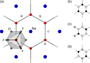
Figure 1: (a) Honeycomb NaIr₂O₆ layer. Iridium ions form a honeycomb lattice with a sodium atom in the middle of each hexagon. Each iridium atom is surrounded by an octahedron of oxygens; the neighboring octahedra share an edge. The figure shows also the definition of cubic $x,y,z$ axes and the bond directions $a,b,c$. (b-d) Sublattices of the two-, four- and six-sublattice transformations $\mathcal{T}_{2},\mathcal{T}_{4},\mathcal{T}_{6}$ that reveal the points of hidden SU(2) symmetry.

II.1 Model Hamiltonian

According to the currently available prevailing evidence for honeycomb materials [15] and following Ref. [80], we choose to study the nearest-neighbor extended Kitaev-Heisenberg model [44; 42; 43] complemented by third-nearest neighbor Heisenberg exchange. The nearest-neighbor (NN) part of the model contains – in addition to the usual Heisenberg exchange – all possible anisotropic terms that are allowed by symmetry of the trigonally distorted honeycomb lattice [44; 75]. It is most conveniently expressed in cubic coordinates $x$, $y$, $z$ introduced in Fig. 1(a) that allow to easily incorporate the discrete rotational $C_{3}$ symmetry. For a bond of $c$ direction, the Hamiltonian contribution reads as

$$\mathcal{H}_{ij}^{(c)}=J\,{\boldsymbol{S}}_{i}\cdot{\boldsymbol{S}}_{j}+K\,S_{i}^{z}S_{j}^{z}\\ \!+\!\Gamma(S_{i}^{x}S_{j}^{y}\!+\!S_{i}^{y}S_{j}^{x})\!+\!\Gamma^{\prime}(S_{i}^{x}S_{j}^{z}\!+\!S_{i}^{z}S_{j}^{x}\!+\!S_{i}^{y}S_{j}^{z}\!+\!S_{i}^{z}S_{j}^{y})$$ (1)

whereas the contributions for the other bond directions are obtained by a cyclic permutation of the spin components $S^{x},S^{y},S^{z}$. The $J$ and $K$ terms alone constitute the Kitaev-Heisenberg model [22; 74] that has been subject to extensive studies [74; 40; 81; 82; 83; 84; 85; 86; 87; 88] and still serves as a prototype model to capture a departure from the Kitaev physics. In light of experimental data [41], it has been generally recognized that further anisotropic terms are needed, leading to the addition of the $\Gamma$ and $\Gamma^{\prime}$ terms introduced in Refs. [42; 43; 44]. When studying the phase diagram we keep signs of $J$ and $K$ flexible and fix the signs $\Gamma>0$ and $\Gamma^{\prime}<0$ following the ab-initio calculations as well as the perturbative evaluation of the effective interactions [47; 43]. According to the latter one, small negative $\Gamma^{\prime}$ should correspond to a trigonal compression of the lattice [43], observed in Na₂IrO₃ [35; 34]. Moreover, several ab-initio studies have evaluated the importance of further-neighbor couplings (see e.g. [45; 47]). In Ref. [47], the effective spin Hamiltonians for Na₂IrO₃, $\alpha$-RuCl₃, and $\alpha$-Li₂IrO₃ were constructed using a combination of DFT and cluster exact diagonalization that equally treated interactions up to third nearest neighbors. Among the further-neighbor interactions, a significant value of $J_{3}>0$ was found for all three compounds, which leads us to the complete model considered here

$$\mathcal{H}=\sum_{\langle ij\rangle\in\mathrm{NN}}\mathcal{H}_{ij}^{(\gamma)}+\!\!\!\sum_{\langle ij\rangle\in 3^{\mathrm{rd}}\,\mathrm{NN}}\!\!\!\!\!\!J_{3}\boldsymbol{S}_{i}\cdot\boldsymbol{S}_{j}\;.$$ (2)

II.2 Hidden symmetries of the model

The NN part of the above model ($J_{3}=0$) has rich symmetry properties explored in detail in the previous work [75]. First, it supports a self-dual transformation $\mathcal{T}_{1}$ that corresponds to a global $\pi$-rotation of the spins around the axis perpendicular to the honeycomb plane. Such a transformation fully preserves the form of the Hamiltonian but replaces the values of the parameters $JK\Gamma\Gamma^{\prime}$ by another set of values. Second, Ref. [75] has also identified a number of special parameter combinations – the points of “hidden” SU(2) symmetry in the parameter space – for which the NN model maps to ferromagnetic (FM) or antiferromagnetic (AF) Heisenberg model on the honeycomb lattice. This is achieved by employing either two-, four-, or six-sublattice coverings of the honeycomb lattice as depicted in Fig. 1(b)-(d) and performing selected sublattice-dependent rotations of the spins. The neighboring spins that belong to different sublattices are therefore rotated in a different fashion and the interaction among those spins takes a modified form, in certain cases the simple Heisenberg one. For these particular cases, the seemingly anisotropic model is thus exactly equivalent to the Heisenberg model on the honeycomb lattice. By using the same transformation backwards, we can exploit the known properties of Heisenberg model obtaining thereby e.g. the ordering pattern or excitation spectra at the points of “hidden” SU(2) symmetry. Due to the sublattice structure of the transformation, the simple ordering patterns of Heisenberg FM or AF transform to more complex ones such as stripy, zigzag or even non-collinear vortex pattern.

As a well-known example, we can consider the Kitaev-Heisenberg model with the parameters satisfying the relation $K=-2J$ and the four-sublattice covering shown in Fig. 1(c). Keeping the spins at the sites marked by $\square$ unrotated, and applying $\pi$-rotations around the $x$, $y$, or $z$ axes to the spins at the sites attached to the $\square$ sites by the $a$, $b$, or $c$ bond, respectively, we obtain the Heisenberg Hamiltonian $\mathcal{H}=-J\sum_{\langle ij\rangle}{\boldsymbol{S}^{\prime}}_{i}\cdot{\boldsymbol{S}^{\prime}}_{j}$ in the rotated spin variables $\boldsymbol{S}^{\prime}$. In the notation of Ref. [75], this transformation is called $\mathcal{T}_{4}$. The other possibilities include two-sublattice transformation $\mathcal{T}_{2}$, the six-sublattice $\mathcal{T}_{6}$, and the combinations $\mathcal{T}_{1}\mathcal{T}_{4}$ and $\mathcal{T}_{2}\mathcal{T}_{6}$. All these points of “hidden” SU(2) symmetry summarized in Table I and Fig. 3 of Ref. [75] provide exact reference points in the parameter space and will be extensively utilized in the present study.

III Methods

To solve the model, we use the standard Lanczos exact diagonalization (ED) technique employing a finite cluster [89]. The calculated cluster ground state is subsequently analyzed utilizing spin-$\frac{1}{2}$ coherent states [80] as detailed below. The ED technique is complemented by the cluster mean-field theory (CMFT). This combination is useful for a global characterization of the phase diagram – ED gives the ground state characteristics such as energies and spin correlations, the analysis based on spin-$\frac{1}{2}$ coherent states enables to better assess the ordering patterns and the direction of magnetic moments, and CMFT supplements this information by the length of the ordered moments which is not directly accessible by ED.

In both cases we use a hexagonal 24-site cluster with periodic boundary conditions applied. This cluster has a fully symmetric shape and supports all the phases with hidden SU(2) symmetry [75]. It is therefore expected to provide a fair environment for the competition of the phases, with the exception of the possible spiral phases that are forced to fit the periodic boundary conditions and may be thus slightly suppressed. In this specific case we have extended our ED analysis to 32-site clusters.

III.1 Spin-$\frac{1}{2}$ coherent states for non-collinear phases

The analysis of the exact ground state of the cluster obtained by ED presents a challenge – the cluster ground state does not spontaneously break symmetry but instead contains a linear combination of all the degenerate spin configurations. To resolve the dominant configuration and obtain the direction of the pseudospins from the ED ground state, we follow Ref. [80] and employ spin-$\frac{1}{2}$ coherent states. Such a state, polarized in a direction given by spherical angles $\theta,\phi$ is given by:

$$|\theta,\phi\rangle=e^{-i\phi S^{z}}e^{-i\theta S^{y}}|\!\uparrow\,\rangle,$$ (3)

where we make a standard choice of cubic $z$ direction as the quantization axis. The cluster spin-coherent state is then a direct product of coherent states on each site $j$:

$$|\Psi\rangle=\prod_{j=1}^{N}|\theta_{j},\phi_{j}\rangle.$$ (4)

This state can be understood as a classical (fluctuation-free) spin pattern with the individual spins pointing in the directions determined by the angles $\theta_{j},\phi_{j}$. By calculating the overlap $\langle\Psi|\mathrm{GS}\rangle$ and maximizing its absolute value by varying the angles, we can identify the classical pattern that best fits the exact ground state $|\mathrm{GS}\rangle$.

For collinear phases (in the case of EKH model, these are FM, AF, zigzag and stripy) the cluster spin-coherent state is captured by a single pair $(\theta,\phi)$, which makes it easy to find the moment direction by inspecting the probability map $P(\theta,\phi)=|\langle\Psi|\mathrm{GS}\rangle|^{2}$ and finding the maximum. However, already the analysis of hidden SU(2) points revealed the existence of several non-collinear “vortex” phases in the phase diagram of the EKH model [75]. In the general case, the probability $P=|\langle\Psi|\mathrm{GS}\rangle|^{2}$ has to be maximized with respect to all $2N$ angles. For our cluster with $N=24$ sites, this poses a nontrivial computational problem of global optimization in 48-dimensional space. To this end, we use the particle swarm method for global optimization, which yields a result further refined by a local optimization algorithm.

The demanding task can be partly avoided by estimating in advance the parameter windows where non-collinear phases can be found. This can be achieved by first finding the optimal spin configuration among the collinear ones and calculating the full Hessian matrix of second derivatives (with respect to all 48 angular parameters) for such a configuration. The potential instability of the collinear phase can be identified by analyzing the eigenvalues of this Hessian matrix.

III.2 Cluster mean-field theory

Similarly to ED, within CMFT we periodically cover the lattice by copies of a given cluster. The bonds connecting the cluster copies (external bonds) are treated in a mean-field approximation, replacing the contributions to the bond Hamiltonian according to the recipe

$$S^{\alpha}_{i}S^{\beta}_{j}\approx\langle S^{\alpha}_{i}\rangle S^{\beta}_{j}+S^{\alpha}_{i}\langle S^{\beta}_{j}\rangle-\langle S^{\alpha}_{i}\rangle\langle S^{\beta}_{j}\rangle,$$ (5)

while the internal bonds of the cluster are kept fully quantum [81]. The mean-field approximation generates effective magnetic fields acting at the outer sites of the cluster and polarizing the cluster ground state to be determined by ED. The polarizing fields depend on the averages $\langle S^{\alpha}_{i}\rangle$ measured on the polarized ground state which leads to a selfconsistent problem with much higher computational demands than the pure ED. On the other hand, by explicitly breaking the ground state symmetry, the CMFT method allows to directly determine the ordering pattern and estimate the ordered moment length.

The introduction of the mean-field boundary makes the sites of the cluster nonequivalent. In combination with the highly anisotropic bond-dependent interactions, the spin structures show a tendency towards various forms of artificial canting. To prevent this, we limit ourselves to the case of collinear spin structures and follow the approach described in Ref. [81], where an averaged ordered moment through the cluster is taken and distributed on the boundary sites following a particular ordering pattern.

IV Global phase diagram

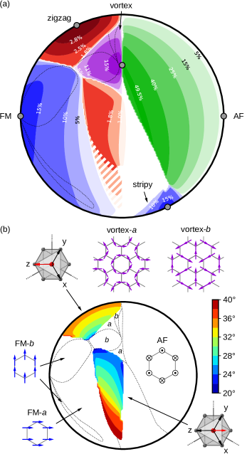
Figure 2: (a) Phase diagram of the extended Kitaev-Heisenberg model with $\Gamma^{\prime}=J_{3}=0$ using the parametrization $J=\cos\varphi\sin\theta$, $K=\sin\varphi\sin\theta$, $\Gamma=\cos\theta$ with $\varphi\in[0,2\pi]$ being the azimuthal angle and $\theta\in[0,\pi/2]$ the radial coordinate measured as a distance from the center of the circle. Color intensity and contours show the probabilities of classical spin patterns for the respective phases. Dashed lines separate distinct regions within one phase. White areas represent regions where no clear signatures of a long-range ordered phase were detected using the 24-site cluster. The gray dots indicate points of (hidden) SU(2) symmetry. The hatched part of the central region with a large probability of the zigzag pattern shows a tendency to form a non-collinear spin arrangement. (b) The angle of the ordered moments to the honeycomb plane for the zigzag phase – in the upper region, the moment points near the cubic $z$ direction (assuming zigzags running along $a$ and $b$ bonds), whereas in the central region it is located between $x$ and $y$ axes. The panel also depicts the in-plane spin patterns for distinct regions (labeled as a and b) within vortex and FM phases and the out-of-plane pattern of the AF phase. Further details can be found in Fig. 9(e) of Appendix C.

By optimizing the spin configurations using the methods described in the previous section and evaluating the corresponding probabilities, we are able to construct a detailed phase diagram of the model. We present the slices through the phase diagram using a common parametrization for the main interactions [42], that is $J=\cos\varphi\sin\theta$, $K=\sin\varphi\sin\theta$, $\Gamma=\cos\theta$ with $\varphi\in[0,2\pi]$ and $\theta\in[0,\pi/2]$. This way all the $J$, $K$ sign combinations and interaction strength ratios for positive $\Gamma\geq 0$ are explored. The remaining model parameters $\Gamma^{\prime}$ and $J_{3}$ are kept fixed for a given slice. Fig. 2(a) shows the phase diagram for $\Gamma^{\prime}=J_{3}=0$, which is the special case of the $JK\Gamma$ model, first analyzed in Ref. [42]. We shall now use this diagram to survey the main properties of the phases and move on to their evolution with $\Gamma^{\prime}$ and $J_{3}$ afterwards. The reader may also consult Appendix C containing an extensive set of phase diagram slices for selected $\Gamma^{\prime}$ values.

IV.1 Collinear phases of the $JK\Gamma$ model

We first focus on the simpler collinear phases which occupy most of the phase diagram. Two phases, FM and AF, dominating Fig. 2(a) are directly linked to Heisenberg points. Though they may seem trivial at the first sight, our inspection revealed their interesting internal structure due to the complex interplay of the bond-anisotropic interactions. We start with the FM phase, which is expected to be most accessible due to the small amount of quantum fluctuations. In the $JK$ limit (the outer circle of the diagram), the ordered moments point along one of the three cubic directions $x,y,z$ selected by virtue of the “order-from-disorder” mechanism on top of isotropic classical energy [90; 80]. Since the cluster ground state is a superposition of the six degenerate possibilities, the probability approaching the value $\frac{1}{6}$ near the FM point indicates vanishing quantum fluctuations. With the presence of the $\Gamma$ term, the magnetic moment is quickly pushed into the honeycomb plane, lying either directly within the plane or close to it (with $\lesssim 10^{\circ}$ deviation, see also Fig. 9(e) in Appendix C). This can be understood by evaluating the classical energy for the FM phase: $E_{\mathrm{class}}\propto 3J+K-\Gamma+\Gamma(n_{x}+n_{y}+n_{z})^{2}$, where the unit vector $\boldsymbol{n}=(n_{x},n_{y},n_{z})$ represents the moment direction. The honeycomb plane is thus preferred by $\Gamma$ interaction on a classical level which makes it easy to outweigh the fluctuation-selected cubic axis. A small $\Gamma$ value of the order $10^{-2}$ to $10^{-1}$ of the dominant $JK$ is typically sufficient to achieve this with the value dropping even lower near the FM Heisenberg point. Within the honeycomb plane, moments point either in the bond direction, or perpendicular to the bond in two separate regions of the FM phase [see Fig. 2(b)]. In accord with the intuition, departing from the FM Heisenberg point, quantum fluctuations intensify, lowering thus the plotted probability.

Linked to the FM phase by means of the four-sublattice transformation ($\mathcal{T}_{4}$ in the notation of Ref. [75]) is the stripy phase. Its hidden FM nature is manifested by a large probability, reaching $\frac{1}{6}$ at the hidden SU(2) point $K=-2J<0$ that is an image of the FM Heisenberg point in the $\mathcal{T}_{4}$ mapping. In contrast to the FM phase, the magnetic moment direction is tied to the vicinity of the cubic axes throughout the stripy phase, lifting a bit with increasing $\Gamma$ instead of moving to the honeycomb plane. This is because the $\Gamma$ interaction is not compatible with the $\mathcal{T}_{4}$ transformation and acts differently here.

In the AF phase, the moment direction is classically degenerate in the $JK$ limit, and the cubic directions are chosen again by the “order-from-disorder” mechanism. The addition of the $\Gamma$ anisotropy fixes now the moments in the $(111)$ direction – perpendicular to the honeycomb plane. This state minimizes the classical energy including $\Gamma$ contribution: $E_{\mathrm{class}}\propto-3J-K+\Gamma-\Gamma(n_{x}+n_{y}+n_{z})^{2}$. Similarly to the FM phase, the fluctuation energy selecting the cubic directions is small and the change to the $(111)$ direction occurs already at a minute $\Gamma$ of the order $10^{-4}$ to $10^{-2}$ of the dominant $JK$ with the critical value of $\Gamma$ decreasing to zero at the AF Heisenberg point. Going deeper into the AF phase, the probability of the classical Néel configuration increases with $\Gamma$ steadily, peaking at $\frac{1}{2}$ on a line near the circle center that starts at the $K=\Gamma$ hidden SU(2) symmetry point. For the (111) AF state, there are two equivalent configurations of the moments, meaning that the peaking probability of 50% represents a classical state without any quantum fluctuations. Indeed, as we later explicitly demonstrate in Sec. V, terms that would lead to quantum fluctuations are present but their remarkable cancellation for the particular order causes the highly anisotropic model to support a fluctuation-free AF state on an entire manifold of its parameter space. The same AF phase may thus be represented by fluctuation-free ground states as well as those with significant quantum fluctuations, depending on the location in the parameter space.

Analogous to the FM/stripy case, $\mathcal{T}_{4}$ maps the AF Heisenberg point to the hidden SU(2) point $K=-2J>0$. The top zigzag region of the phase diagram extends around this point; in the $JK$ limit, the moment direction coincides again with one of the cubic directions. Adding further anisotropy with increasing $\Gamma$, the moments are pushed continuously towards the honeycomb plane, as shown in Fig. 2(b).

Of a greater experimental relevance is the second zigzag phase near the center of the phase diagram. It is also linked to a hidden SU(2) point which, however, occurs at finite $\Gamma^{\prime}<0$ [75]. In this phase, the moment direction is located roughly between the cubic $x$ and $y$ axes, near the direction found experimentally [41]. We will show later, that it is this zigzag region that largely expands and dominates the phase diagram after the inclusion of $\Gamma^{\prime}$ and/or $J_{3}$ coupling terms. A comprehensive discussion of the moment direction in both zigzag phases in the context of the experimental data can be found in Ref. [80].

IV.2 Vortex phase

The vortex phase is a non-collinear phase “emanating” from the most peculiar hidden SU(2) symmetry point of the model that is revealed by a six-sublattice spin rotation $\mathcal{T}_{6}$ of Ref. [75]. $\mathcal{T}_{6}$ maps the ferromagnetic $J<0$ Heisenberg model to EKH model at the parameter point $J=0$, $K=\Gamma>0$ indicated in Fig. 2(a). Owing to its hidden FM nature and six degenerate spin configurations, the optimized probabilities reach $\tfrac{1}{6}$ in the vicinity of this exact vortex point, and continuously decrease with the departure away from it.

The phase comprises regions with two different most probable classical configurations of moments labeled as vortex-a and vortex-b in Fig. 2(b). Let us note, however, that these two patterns have very close probabilities and are continuously connected, implying a presence of a soft mode oscillating between them. In partial agreement with the classical treatment [42], spins are found to lie within or close to the honeycomb plane. The vortex-b pattern is always planar while in the vortex-a regions near the boundary with AF or zigzag phase, the spins start to tilt away from the honeycomb plane in a staggered AF fashion. The tilt is largest in the right part of the vortex phase [see Fig. 9(e)] which we interpret as the proximity effect of the robust AF order with the moments perpendicular to the honeycomb plane.

A deeper understanding of the internal structure of the vortex phase is possible by utilizing four reference points where the EKH maps to simpler models. One of them is the vortex SU(2) point in $\Gamma^{\prime}=0$ slice. The freedom associated with the selection of the ordered moment direction in the hidden FM at this point creates a continuous family of degenerate patterns including vortex-a and vortex-b. Another hidden SU(2) symmetry point but of AF nature is found for $\Gamma^{\prime}\approx-0.5$ at the opposite edge of the vortex phase [see Fig. 9(j) of Appendix C]. It is associated with $\mathcal{T}_{2}\mathcal{T}_{6}$ transformation of Ref. [75]. For a planar structure, the staggering of the hidden AF order is compensated by the two-sublattice $\pi$-rotation $\mathcal{T}_{2}$ such that this point supports the same vortex-a and vortex-b patterns as for the $\Gamma^{\prime}=0$ hidden FM point associated with just $\mathcal{T}_{6}$. However, in contrast to the latter point, the corresponding state has pronounced quantum fluctuations because of the hidden AF nature. Departing away from the hidden FM point or the hidden AF point, the degeneracy is lifted and one of the configurations is chosen as the energetically most favorable. Here the proximity to the remaining two reference points decides. As we find in Sec. VI, the point $K=\Gamma=-J>0$ (the “meeting” point of four phases) corresponds to a FM compass model on the honeycomb lattice while at another nearby point with $K>0$, $J=\Gamma>0$, and $\Gamma^{\prime}<0$, the model maps to AF compass-like model with the interaction direction perpendicular to the bond. These two compass(-like) models prefer patterns vortex-b and vortex-a, respectively, which qualitatively explains the location of vortex-a,b subphases.

IV.3 Remaining phases of the $JK\Gamma$ model

The remaining parts of the phase diagram slice for $\Gamma^{\prime}=0$ and $J_{3}=0$ [kept white in Fig. 2(a)] are to a small extent occupied by the two known Kitaev spin liquids associated with the FM and AF Kitaev points. Here the optimization of spin-$\frac{1}{2}$ coherent states described in Sec. III.1 finds a large number of configurations consisting of aligned/contra-aligned pairs of the nearest-neighbor spins, as appearing in classical $S\rightarrow\infty$ limit of the Kitaev model [91; 92] (see also Appendix A for several details concerning the behavior of the method in the presence of Kitaev spin liquids).

However, much bigger portion of the phase diagram is taken by the white region in the lower central part which shows a particularly puzzling behavior. Parts of it were suggested earlier to host incommensurate phases [42; 78]. The vertical $J=0$ line seems to play a special role as it clearly separates the middle zigzag as well as the vortex region from the other phases on the right [see Fig. 2(a) and the detail in Fig. 3(a)]. The $K-\Gamma$ model corresponding to the $J=0$ line has been recently studied separately and its ground state for ferromagnetic $K$ was found to bear signatures of a spin liquid [93; 94].

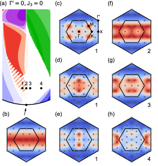
Figure 3: (a) Position of the four selected points $1-4$ in the phase diagram. In addition, the FM Kitaev point is taken as a reference. (b)–(h) $\langle S_{-\boldsymbol{q}}^{z}S^{z}_{\boldsymbol{q}}\rangle$ correlations at the selected parameter points calculated for the 24-site cluster (b,c,f,g) and 32-site clusters of hexagonal (d,h) and rectangular shape (e). The nearest-neighbor correlations in the liquid state are manifested by a wave-like pattern [panel (b)] – such a pattern seems to be present as a “background” in the other maps (c–h) as well. At point $1$, the larger 32-site clusters already support incommensurate correlations [panels (d),(e)], while the 24-site cluster shows zigzag-like correlations [panel (c)] though collinear zigzag is not the most probable configuration anymore. Incommensurate correlations are visible at the 24-site cluster for point $3$ [panel (g)] and merge with the zigzag ones on the $K-\Gamma$ line [panel (f)]. Deeper in the white region, the incommensurate wavevector moves out of the first Brillouin zone [panel (h)]. All the panels (b–h) show the available $\boldsymbol{q}$-resolution for the given cluster. In panel (c), the high-symmetry points in the Brillouin zone are labeled.

Using the method of Sec. III.1 for the above region, we find tendencies to form complex spin structures, though the probability of such configurations is quite small, hinting towards a possibility of phase(s) without a long-range order. Interestingly, the region with a large probability of the collinear zigzag structure is also partially unstable towards a formation of a non-collinear spin arrangement – see the hatched pattern in Fig. 2(a) or Fig. 3(a). Although the clusters accessible to ED are not in general large enough to properly capture potential spin orderings with large unit cells, we still try to provide a further analysis based on momentum-space correlations. Here we utilize two more clusters in ED, a 32-site cluster of a hexagonal shape and a rectangular one ($4\sqrt{3}\times 6$ in lattice spacings), in addition to our default 24-site cluster.

Fig. 3(a) shows the positions of four parameter points selected for a comparison: $1$ in the unstable zigzag region, $2$ on the $K-\Gamma$ boundary, $3$ in the expected spiral phase close to $J=0$ line, and point $4$ deeper in the expected spiral phase. The FM Kitaev point is added for reference. Plotted in Fig. 3(b)–(h) are the maps of the equal-time spin-spin correlation function $\langle S_{-\boldsymbol{q}}^{z}S^{z}_{\boldsymbol{q}}\rangle$. It should be emphasized, that the cluster ground states do not spontaneously break symmetry and contain e.g. a linear combination of several ordering patterns that differ by the direction of the ordering wavevector and hence the ordered moment direction. The selection of the spin component of the correlation function then provides access to various components of this combination. For the hexagonal clusters, where a rotation by $2\pi/3$ is in effect just a cyclic permutation among the $S^{x}$, $S^{y}$, and $S^{z}$ components, the other correlation functions $\langle S_{-\boldsymbol{q}}^{x}S^{x}_{\boldsymbol{q}}\rangle$ and $\langle S_{-\boldsymbol{q}}^{y}S^{y}_{\boldsymbol{q}}\rangle$ are merely $2\pi/3$-rotated copies of the maps shown in Fig. 3.

By combining various sets of maps from Fig. 3, several trends can be illustrated:
(i) The wave-like background identical to momentum-represented nearest-neighbor correlations of the Kitaev liquid [Fig. 3(b)] is universally present at all points, less apparently in the case of peaked structures on top of the background because of an extended colorscale range.
(ii) Panels (c), (d), and (e) show the influence of the cluster size and shape at the parameter point $1$ that we demonstrate now to be in the incommensurate region. For the smallest 24-site cluster, the correlation map in Fig. 3(c) still includes peaks located at the $M$ momenta which corresponds to a zigzag arrangement. However, using the method of Sec. III.1, the zigzag pattern is found unstable which already hints towards another type of ordering. This is fully revealed by the larger 32-site clusters. By providing a denser momentum-space coverage, they enable the preferred incommensurate state to develop [Figs. 3(d),(e)]. The difference between Fig. 3(d) and Fig. 3(e) is an effect of the cluster shape. The symmetric hexagonal 32-site cluster [panel (d)] supports three degenerate directions for the ordering wavevector that coexist in the ground state (two of them visible aside the main maxima near the Brillouin zone center), while the rectangular shape of the second 32-site cluster selects only one of those directions [panel (e)].
(iii) Panels (c), (f), and (g) demonstrate, for the 24-site cluster, the evolution from commensurate correlations [point 1, Fig. 3(c)] to incommensurate ones [point 3, Fig. 3(g)] found in the white region. At the boundary point $2$ with $J=0$, the corresponding states show a level crossing and we obtain the average spin-correlation pattern displayed in Fig. 3(f) resembling that of the Kitaev point.
(iv) Panels (d) and (h) illustrate, for the symmetric 32-site cluster, the transfer of the incommensurate wavevector from the inside of the first Brillouin zone [point $1$, Fig. 3(d)] to the outside [point $4$, Fig. 3(h)] when moving in the direction of positive $J$. This trend was also obtained by classical Monte-Carlo simulations [43].

In conclusion, the studied region of the phase diagram shows a complex behavior with the spin-correlations indicating tendencies towards various incommensurate orders. However, the common wave-like background to the spin-correlations suggests a presence of strong liquid-like features.

IV.4 Effect of nonzero $\Gamma^{\prime}$ and $J_{3}$ parameters

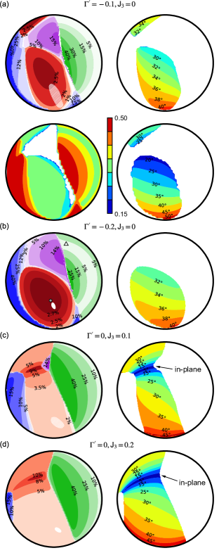
Figure 4: Phase diagrams for nonzero values of $\Gamma^{\prime}$ and $J_{3}$ represented by probabilities of optimized collinear and vortex spin patterns in the ED ground state (left) and, focusing on zigzag phases, by the angle of the moments to the honeycomb plane (right). Hatched/white areas in the zigzag phase indicate the instability of the collinear pattern. Bottom part of panel (a) also shows the ordered moment length calculated by CMFT (left) and the angle to the honeycomb plane in zigzag phases (right). Shown in panel (b) are projected positions of a hidden SU(2) point (gray •) and a compass-like point ($\vartriangle$).

We shall now investigate the evolution of the phases found in the $\Gamma^{\prime}=J_{3}=0$ slice of the phase diagram when the parameters $\Gamma^{\prime}$ and $J_{3}$ are varied. As argued in Sec. II, we limit ourselves to the experimentally most relevant case of small $\Gamma^{\prime}<0$ and $J_{3}>0$. Additional data to establish a fuller picture are presented in Appendix C. The observed trends can be successfully explained either simply by considering the classical energy or, more fundamentally, correlated with the positions of the points of special symmetry in the parameter space, as inspected in Ref. [75] (points of hidden SU(2) symmetry) and the following sections V and VI.

Fig. 4(a),(b) shows phase diagrams for two moderate values of $\Gamma^{\prime}<0$. Most notable effect of negative $\Gamma^{\prime}$ is the large expansion of the vortex phase and mainly of the central zigzag phase. The former trend can be understood as a proximity effect of the point where the EKH model maps to AF compass-like model (to be analyzed in Sec. VI). Its position is at $\Gamma^{\prime}\approx-0.6$ in the chosen parametrization and the projection to $JK\Gamma$ plane is indicated in Fig. 4(b). Though the difference in $\Gamma^{\prime}$ is still quite large, this special point efficiently enforces the vortex-like correlations of type a so that the vortex phase not only grows but also becomes dominated by vortex-a pattern (c.f. Appendix C). The expansion of the central zigzag phase is linked to approaching the hidden SU(2) point that is an image of the AF Heisenberg point in $\mathcal{T}_{1}\mathcal{T}_{4}$ transformation. This point, having $\Gamma^{\prime}\approx-0.4$ and the projection onto $JK\Gamma$ plane as indicated in Fig. 4(b), enforces the zigzag order with the moment direction consistent with experiments and may be actually regarded as the source of the central zigzag phase. On the other hand, the top zigzag region related to the SU(2) point in the $\Gamma^{\prime}=0$ plane is suppressed with $\Gamma^{\prime}<0$, to the extent that it is not even discernible already for $\Gamma^{\prime}=-0.2$.

The FM and AF phases develop more complex internal structure when $\Gamma^{\prime}<0$ is added. This is due to the competition of the energy contributed by $\Gamma$ and $\Gamma^{\prime}$ that are decisive for the moment direction at a classical level. The anisotropic part of these contributions is proportional to $\pm(\Gamma+2\Gamma^{\prime})(n_{x}+n_{y}+n_{z})^{2}$ for FM and AF, respectively. In the FM phase, $\Gamma^{\prime}<0$ creates a new subphase where the moments pushed originally to the honeycomb plane due to $\Gamma>0$ [Fig. 2(b)] take the direction perpendicular to the honeycomb plane. This subphase extends near the outer rim of the FM phase where $\Gamma$ is sufficiently weak. An opposite effect is observed in the AF phase. Here, in addition, the absence of the moment confinement by anisotropic classical energy in the case of $\Gamma+2\Gamma^{\prime}=0$ leads to an enhancement of quantum fluctuations and the probability plotted in e.g. Fig. 4(b) therefore drops at the corresponding circle.

Based on the data presented so far, the probabilities of the best-fitting classical configurations represent a good measure of quantum fluctuations in the ground state. To have an independent quantification and to cross-check our results, we compare them to a complementary approach, namely CMFT described in Sec. III.2. Its advantage is the ability to estimate the ordered moment length that we plot in Fig. 4(a). The phase boundaries of the collinear phases are in a good agreement with the method based on ED and the moment length reveals the less fluctuating FM and stripy phases, and the gradual decrease of quantum fluctuations when going deeper into the AF phase. The data on the moment angle to the honeycomb plane shows a somewhat larger spread but the trend is identical.

The evolution of the phases with increasing third nearest-neighbor coupling $J_{3}$ is illustrated in Fig. 4(c),(d). As expected already at the level of the classical energy, the antiferromagnetic $J_{3}>0$ coupling further favors zigzag and AF phases. The stripy and vortex phases of hidden FM nature as well as the FM phase get quickly suppressed and the two zigzag regions merge filling the entire left half of the phase diagram. In both zigzag and AF phases, the third nearest-neighbor bonds have contra-aligned spins favorable for AF $J_{3}$ interaction. The energy gain brought by $J_{3}$ therefore does not visibly shift the zigzag/AF boundary. The two zigzag regions have incompatible moment directions. When merging them, the system makes a compromise by pushing the moment direction to the honeycomb plane so that it can easily flip between $z$ and $(x+y)/\sqrt{2}$ directions projected onto honeycomb plane [c.f. Fig. 2(b)]. Near the boundary between the zigzag subphases where the moment lies in the honeycomb plane, the quantum fluctuations are significantly suppressed.

We reach the conclusion that both $\Gamma^{\prime}<0$ and $J_{3}>0$ – expected to be present in real materials – strongly stabilize the central zigzag phase that is consistent with experimental observations in Na₂IrO₃ in both the magnetic ordering and direction of magnetic moment. As for the precise moment direction (figures in the right column of Fig. 4), the evolution seems to be dictated by $K$, $\Gamma$, while $\Gamma^{\prime}$, $J_{3}$ influence mostly the extent of the phase. We note that one has to distinguish the real pseudospin direction and the moment direction as probed by various techniques such as neutron or resonant x-ray scattering [80]. Based solely on the moment direction with the experimental data [41] translating to the pseudospin angle of about $38^{\circ}-40^{\circ}$ [80], it seems that the FM $K<0$ should be the largest interaction, followed by possibly still large $\Gamma>0$. Being in accord with the conclusions of Ref. [80], this also falls in line with ab-initio estimates of dominant ferromagnetic $K$ and comparable $J>0,\Gamma>0,\Gamma^{\prime}<0$ and $J_{3}>0$ [15].

Finally, small hatched/white areas in the zigzag phase shown in Fig. 4 again indicate the instability of the collinear zigzag pattern that may be interpreted as a protrusion of the possible incommensurate phase. They appear at small $\Gamma^{\prime}$ and $J_{3}$ which together with the link between $\Gamma^{\prime}$ and trigonal distortion suggests an explanation for the spiral order in less distorted $\alpha$-Li₂IrO₃ compared to Na₂IrO₃ with zigzag order. This point was analyzed at a basic classical level in Ref. [75].

V Fluctuation-free manifolds

As noticed in Sec. IV.1 when inspecting the phase diagram of the $JK\Gamma$ model [Fig. 2(a)], the AF phase contains an unusual line of fluctuation-free ground states located near the center of the phase diagram. The distance to this line seems to determine the magnitude of quantum fluctuations throughout the entire AF phase – the probability of the Néel state in the ground state increases more or less monotonously starting from the outer rim and approaching the line radially inwards. In fact, similar lines are present also for nonzero $\Gamma^{\prime}$ slices in a certain $\Gamma^{\prime}$ range and form thus an entire surface in the parameter space. This is quite unexpected since at those parameter points, all the interactions are active and there is no apparent cancellation leading to the absence of quantum fluctuations. What is more, a manifold of fluctuation-free ground states is found also in part of the FM phase away from the trivially fluctuation-free FM Heisenberg point. This is demonstrated in Fig. 5(a) for two values of $\Gamma^{\prime}<0$. Below we address both cases, starting with the simpler FM one.

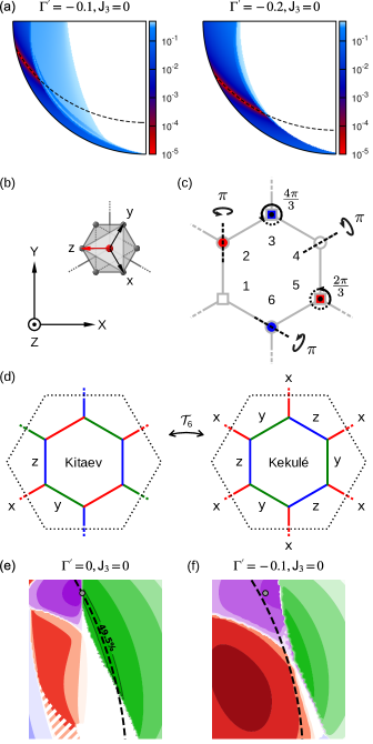
Figure 5: (a) Lower left quadrant of the phase diagram for $\Gamma^{\prime}=-0.1$ and $\Gamma^{\prime}=-0.2$ showing the FM phase. The color indicates the difference $P_{\mathrm{max}}-P$ between the probability $P$ of the classical state in the ED ground state and its maximum value of $P_{\mathrm{max}}=\frac{1}{2}$. The maximum probability, corresponding to a fluctuation-free ground state, is reached in the FM subphase with the moments perpendicular to the honeycomb plane (darker color) at the line given by $K+2\Gamma-2\Gamma^{\prime}=0$ (dashed). (b) Coordinate frames used to express spin interactions. (c) Schematic representation of the $\mathcal{T}_{6}$ transformation on the honeycomb lattice. At each of the six sublattices, a different rotation of spin components is applied. (d) Correspondence between the bonds and interaction Hamiltonians $\mathcal{H}^{(x)}$, $\mathcal{H}^{(y)}$, $\mathcal{H}^{(z)}$ for the EKH model and extended Kekulé-Kitaev-Heisenberg model obtained when performing the $\mathcal{T}_{6}$ transformation. (e) The fluctuation-free line in the AF phase of the $JK\Gamma$ model. The line is determined by $3J+K-\Gamma-2\Gamma^{\prime}=0$ and crosses the hidden SU(2) symmetric vortex point (gray •). (f) Shifted line for a case of non-zero $\Gamma^{\prime}$: the line no longer enters the AF phase.

V.1 FM phase

A common feature of the fluctuation-free ground states is the moment direction being perpendicular to the honeycomb plane, suggesting to rewrite the Hamiltonian into the $XYZ$ reference frame [Fig. 5(b)] where this perpendicular direction is singled out. The Hamiltonian contributions for all the bond directions can be cast to a common form [75]:

$$\mathcal{H}^{(\gamma)}_{ij}=J_{XY}(S_{i}^{X}S_{j}^{X}+S_{i}^{Y}S_{j}^{Y})+J_{Z}S_{i}^{Z}S_{j}^{Z}$$

$$+A\,[(S_{i}^{X}S_{j}^{X}\!-\!S_{i}^{Y}S_{j}^{Y})\cos\phi_{\gamma}-(S_{i}^{X}S_{j}^{Y}\!+\!S_{i}^{Y}S_{j}^{X})\sin\phi_{\gamma}]$$

$$-B\,[(S_{i}^{X}S_{j}^{Z}\!+\!S_{i}^{Z}S_{j}^{X})\cos\phi_{\gamma}+(S_{i}^{Y}S_{j}^{Z}\!+\!S_{i}^{Z}S_{j}^{Y})\sin\phi_{\gamma}].$$ (6)

The bond-dependence of the interactions is expressed via the trigonometric factors containing the angles of the bonds measured from the $Y$ axis, i.e. $\phi_{\gamma}=0,\frac{2\pi}{3},\frac{4\pi}{3}$ for the $c$, $a$, and $b$ bonds, respectively. Eq. (V.1) is obtained by inserting into Eq. (1) the transformation relations

$$\begin{pmatrix}S^{x}\rule{0.0pt}{0.0pt}\\ S^{y}\rule{0.0pt}{14.22636pt}\\ S^{z}\rule{0.0pt}{14.22636pt}\end{pmatrix}=\begin{pmatrix}\frac{1}{\sqrt{6}}&-\frac{1}{\sqrt{2}}&\frac{1}{\sqrt{3}}\rule{0.0pt}{0.0pt}\\ \frac{1}{\sqrt{6}}&\frac{1}{\sqrt{2}}&\frac{1}{\sqrt{3}}\rule{0.0pt}{14.22636pt}\\ -\sqrt{\tfrac{2}{3}}&0&\frac{1}{\sqrt{3}}\rule{0.0pt}{14.22636pt}\end{pmatrix}\begin{pmatrix}\phantom{-}S^{X}\!\cos\phi_{\gamma}+S^{Y}\!\sin\phi_{\gamma}\rule{0.0pt}{0.0pt}\\ -S^{X}\!\sin\phi_{\gamma}+S^{Y}\!\cos\phi_{\gamma}\rule{0.0pt}{14.22636pt}\\ S^{Z}\rule{0.0pt}{14.22636pt}\end{pmatrix}$$ (7)

which represent a conversion from the cubic $xyz$ to $XYZ$ reference frame for a $c$ bond as well as the necessary cyclic permutation among $xyz$ (rotation around $Z$ axis), and using the fact that $\cos 2\phi_{\gamma}=\cos\phi_{\gamma}$, $\sin 2\phi_{\gamma}=-\sin\phi_{\gamma}$ for the allowed values of $\phi_{\gamma}$.

The interaction parameters in (V.1) expressed in terms of the original $J$, $K$, $\Gamma$, and $\Gamma^{\prime}$ read as

$$J_{XY} =J+\tfrac{1}{3}(K-\Gamma-2\Gamma^{\prime}),$$ (8)

$$J_{Z} =J+\tfrac{1}{3}(K+2\Gamma+4\Gamma^{\prime}),$$ (9)

$$A =\tfrac{1}{3}(K+2\Gamma-2\Gamma^{\prime}),$$ (10)

$$B =\tfrac{\sqrt{2}}{3}(K-\Gamma+\Gamma^{\prime}).$$ (11)

Let us now consider a FM state polarized in the $Z$ direction and inspect the terms that could lead to quantum fluctuations. As in usual Heisenberg magnets, the $J_{XY}$ interaction containing $S_{i}^{+}S_{j}^{-}$ and $S_{i}^{-}S_{j}^{+}$ does not act on the polarized state. The above state is an eigenstate of the $S_{i}^{Z}$ operators, the action of $B$-terms in the Hamiltonian therefore sums up to

$$-B\sum_{\mathrm{sites}}\left[S_{i}^{X}\sum_{\gamma=a,b,c}\!\!\cos\phi_{\gamma}+S_{i}^{Y}\sum_{\gamma=a,b,c}\!\!\sin\phi_{\gamma}\right]$$ (12)

which drops out since both $\sum_{\gamma}\cos\phi_{\gamma}$ and $\sum_{\gamma}\sin\phi_{\gamma}$ are zero. Only the remaining $A$-terms containing $S_{i}^{+}S_{j}^{+}$ and $S_{i}^{-}S_{j}^{-}$ are active. Setting $A=0$, all the $S_{i}^{-}$ or $S_{i}^{-}S_{j}^{-}$ terms that could lead to quantum fluctuations are cut off by zero prefactors and we are left with an exact eigenstate. The two conditions for a fluctuation-free FM ground state, i.e. moments being perpendicular to the honeycomb plane and $A=0$ translating to

$$K+2\Gamma-2\Gamma^{\prime}=0,$$ (13)

are checked in Fig. 5(a). Approaching the line given by Eq. (13) within the $(111)$ polarized FM phase, the probability indeed reaches the maximum value of $\frac{1}{2}$, reflecting the two degenerate configurations (moments along $Z$ or $-Z$) being superposed in the cluster ground state. Exactly at this line, we find a doubly degenerate ground state. Finally, let us note that the ground state remains fluctuation-free even in the presence of $J_{3}$ provided that the $(111)$ polarized FM pattern is preserved.

V.2 AF phase

A more complex situation is encountered in the case of $(111)$ polarized AF phase. Here the fluctuation-free manifold is attached to the vortex point of hidden SU(2) symmetry hosting an infinite number of fluctuation-free states. The $(111)$ polarized AF state is one of them, the others being e.g. the vortex-a and vortex-b configurations shown in Fig. 2(b). The connection to the SU(2) vortex point suggests a special role of the $\mathcal{T}_{6}$ transformation which we discuss in more detail here.

The $\mathcal{T}_{6}$ transformation is a 6-sublattice mapping that rotates the spins according to the recipe:

$$\text{sublattice 1:}\quad(S^{x\prime},S^{y\prime},S^{z\prime}) =(S^{x},S^{y},S^{z}),$$

$$\text{sublattice 2:}\quad(S^{x\prime},S^{y\prime},S^{z\prime}) =(-S^{y},-S^{x},-S^{z}),$$

$$\text{sublattice 3:}\quad(S^{x\prime},S^{y\prime},S^{z\prime}) =(S^{y},S^{z},S^{x}),$$

$$\text{sublattice 4:}\quad(S^{x\prime},S^{y\prime},S^{z\prime}) =(-S^{x},-S^{z},-S^{y}),$$

$$\text{sublattice 5:}\quad(S^{x\prime},S^{y\prime},S^{z\prime}) =(S^{z},S^{x},S^{y}),$$

$$\text{sublattice 6:}\quad(S^{x\prime},S^{y\prime},S^{z\prime}) =(-S^{z},-S^{y},-S^{x}).$$ (14)

For a better understanding, the transformation is depicted in Fig. 5(c). On sites $1$, $3$, $5$ marked by a square symbol, the spins are rotated around the $(111)$ axis, on sites $2$, $4$, $6$ marked by a circle, the mapping consists of $\pi$-rotations around axes lying in the honeycomb plane. This in effect changes the $(111)$ polarized AF pattern into $(111)$ polarized FM one, making a first step towards the understanding of the AF fluctuation-free line.

The second step involves the transformation of the Hamiltonian. Performing the $\mathcal{T}_{6}$ spin rotations, we find that the resulting model is similar to EKH in the sense that three types of bond interactions of the form of Eq. (1) appear, $\mathcal{H}^{(x)}\equiv\mathcal{H}^{(a)}$, $\mathcal{H}^{(y)}\equiv\mathcal{H}^{(b)}$, and $\mathcal{H}^{(z)}\equiv\mathcal{H}^{(c)}$, with the parameters modified according to

$$(J,K,\Gamma,\Gamma^{\prime})_{\text{Kekul\'{e}}}=(-\Gamma,-J-K+\Gamma,-J,-\Gamma^{\prime}).$$ (15)

However, the assignment of $\mathcal{H}^{(x,y,z)}$ to the bonds is not simply by the bond direction anymore. Instead, as shown in Fig. 5(d), a network of benzene-like rings governed by alternating $\mathcal{H}^{(y)}$ and $\mathcal{H}^{(z)}$ is formed. They are interconnected by bonds possessing the $\mathcal{H}^{(x)}$ type of interactions. This way, the $\mathcal{T}_{6}$ transformation maps the EKH model to an extended variant of Kekulé–Kitaev model [95].

We are now in position to combine the result of $\mathcal{T}_{6}$ transformation with the argumentation of Sec. V.1. Since the transformation led to $(111)$ polarized FM pattern and in the new model each site is a member of three bonds governed by $\mathcal{H}^{(x)}$, $\mathcal{H}^{(y)}$, and $\mathcal{H}^{(z)}$, the cancellation of the terms leading to quantum fluctuations proceeds exactly the same way. Substituting the parameters in Eq. (13) according to (15), we thus arrive at the condition for the fluctuation-free AF state:

$$3J+K-\Gamma-2\Gamma^{\prime}=0.$$ (16)

As demonstrated in Fig. 5(e), this line coincides with the region where the probability of Néel state peaks at $\frac{1}{2}$. For a negative $\Gamma^{\prime}$, the line quickly gets out of the AF phase. However, going in the positive $\Gamma^{\prime}$ direction, the fluctuation-free line gets even deeper into the AF phase (c.f. Appendix C). At the special point $J=\Gamma=\Gamma^{\prime}>0$, $K=0$ on the fluctuation-free manifold, the model even reduces to AF Ising model with the $(111)$ Ising axis, as can be seen from Eqs. (V.1)-(11).

Unlike in the previous FM case, the addition of $J_{3}$ spoils the fluctuation-free nature of the ground state since the $J_{3}$ interaction generates terms of $A$-type under the $\mathcal{T}_{6}$ transformation.

VI Ising-Kitaev-compass model

In this section, we address yet another feature of the model that enables further insights into its phase behavior. Namely, we find points in the parameter space where the four interactions $JK\Gamma\Gamma^{\prime}$ can be combined into a single one, characterized by a single interacting spin component (interaction axis) that depends on the bond direction. This way, the model in Eq. (V.1) may realize combinations of Ising, Kitaev, or compass model on the honeycomb lattice.

VI.1 Compass point in the phase diagram

Inspecting the $JK\Gamma$ phase diagram, we find a degenerate point, in which several phases seem to meet: vortex, ferromagnet, and both zigzag phases. Writing the interaction as $\mathcal{H}=\sum_{ij}\boldsymbol{S}^{T}_{i}H_{ij}\boldsymbol{S}_{j}$, we find that the Hamiltonian matrices in this parameter point $K=\Gamma=-J>0$, $\Gamma^{\prime}=0$ have a symmetrical block shape:

$$H_{a} =\begin{pmatrix}J+K&\Gamma^{\prime}&\Gamma^{\prime}\\ \Gamma^{\prime}&J&\Gamma\\ \Gamma^{\prime}&\Gamma&J\end{pmatrix}=\begin{pmatrix}0&0&0\\ 0&-K&K\\ 0&K&-K\end{pmatrix},$$ (17)

$$H_{b} =\begin{pmatrix}J&\Gamma^{\prime}&\Gamma\\ \Gamma^{\prime}&J+K&\Gamma^{\prime}\\ \Gamma&\Gamma^{\prime}&J\end{pmatrix}=\begin{pmatrix}-K&0&K\\ 0&0&0\\ K&0&-K\end{pmatrix},$$ (18)

$$H_{c} =\begin{pmatrix}J&\Gamma&\Gamma^{\prime}\\ \Gamma&J&\Gamma^{\prime}\\ \Gamma^{\prime}&\Gamma^{\prime}&J+K\end{pmatrix}=\begin{pmatrix}-K&K&0\\ K&-K&0\\ 0&0&0\end{pmatrix}.$$ (19)

The matrices can be diagonalized by a change of basis to the rotating coordinate frame $\tilde{x}_{\gamma},\tilde{y}_{\gamma},\tilde{z}_{\gamma},\gamma\in\{a,b,c\}$, where $\tilde{x}_{\gamma}$ axis points in the bond direction, $\tilde{y}_{\gamma}$ is perpendicular to the bond direction and lies in the honeycomb plane, and $\tilde{z}_{\gamma}$ points out of the honeycomb plane – see Fig. 6(a) for a sketch of this coordinate system. After the change of basis, all three interaction matrices have the same form for all bond directions $a$, $b$, $c$:

$$\widetilde{H}=\begin{pmatrix}-2K&0&0\\ 0&0&0\\ 0&0&0\end{pmatrix},$$ (20)

which represents FM interaction in the bond direction, concisely written as:

$$\mathcal{H}=\sum_{\langle ij\rangle\in\mathrm{NN}}-2K(\boldsymbol{S}_{i}\cdot\boldsymbol{r}_{ij})(\boldsymbol{S}_{j}\cdot\boldsymbol{r}_{ij}),$$ (21)

where the unit vector $\boldsymbol{r}_{ij}$ points from site $i$ to site $j$. This form of interaction is known in the literature as the 120^∘ honeycomb compass model [96; 97; 98; 11]. Similar to the Kitaev model, it features frustration due to competing interactions for the three bond directions. However, the exact ground state is not known in this case and its nature is in fact not clear, as several past works came to inconsistent conclusions. One study found a Néel state [96], others suggested a stabilization of a dimer pattern [97], a superposition of dimer coverings [98], or a quantum spin liquid state [99]. With the link to the compass model, the apparent special role of the $-J=K=\Gamma$ point marked by a competition of four long-range ordered phases in its vicinity is confirmed. This competition was noticed also in the tensor-network analysis of the $JK\Gamma$ model [77], which claimed a small region surrounding this point to harbor a valence bond solid phase.

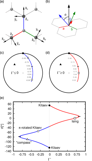
Figure 6: (a) Rotating coordinate system $\tilde{x}_{\gamma},\tilde{y}_{\gamma},\tilde{z}_{\gamma}$ on a honeycomb lattice – color distinguishes three bond types $a$, $b$, $c$. (b) The direction of the interaction axis for each bond. All of them are at an angle $\vartheta$ with the Ising $(111)$ direction shown in black. (c),(d) Ising-Kitaev-compass parameter line in the phase diagram and the corresponding values of the $\Gamma^{\prime}$ parameter. The Ising point ($\Box$) emerges for positive $\Gamma^{\prime}$, while the $\pi$-rotated Kitaev point ($\circ$) and the perpendicular “compass” point ($\vartriangle$) are found for negative $\Gamma^{\prime}$ values. The true compass point ($\blacktriangle$) appears for $\Gamma^{\prime}=0$. (e) The angle $\vartheta$ of the interaction axis to the $(111)$ direction depending on the position on the parameter line. $\varphi=\pi/2$ is assumed. The Kitaev point (•) is connected to the $\pi$-rotated Kitaev point ($\circ$) by the $\mathcal{T}_{1}$ dual transformation [75] – a $\pi$-rotation around the $(111)$ axis.

VI.2 Ising-Kitaev-compass line in the phase diagram

Motivated by the previous example, we now demonstrate that the EKH model provides also a more general case of a single interaction axis lying anywhere between the honeycomb plane and the perpendicular $(111)$ direction. Dictated by the $C_{3}$ symmetry of the EKH model, the interaction axis has to rotate together with the bond direction as shown in Fig. 6(b). Representing the bond-dependent interaction axis by a unit vector $\boldsymbol{n}_{\gamma}$, the Hamiltonian of the single-axis model hidden in the EKH model has to be of the form

$$\mathcal{H}_{\mathrm{IKc}}=\sum_{\langle ij\rangle\in\mathrm{NN}}\widetilde{K}(\boldsymbol{n}_{\gamma}\cdot\boldsymbol{S}_{i})(\boldsymbol{n}_{\gamma}\cdot\boldsymbol{S}_{j}).$$ (22)

We specify the interaction-axis direction by the deviation $\vartheta$ from the $(111)$ direction and the azimuthal angle $\varphi$ measured from the bond. In the rotating reference frame $\tilde{x}_{\gamma}\tilde{y}_{\gamma}\tilde{z}_{\gamma}$ we have

$$\boldsymbol{n}_{\gamma}=\bigl{(}\,\sin\vartheta\cos\varphi,\sin\vartheta\sin\varphi,\cos\vartheta\,\bigl{)}$$ (23)

while in the $XYZ$ reference frame of Fig. 5(b)

$$\boldsymbol{n}_{\gamma}=\bigl{(}\,-\sin\vartheta\sin(\varphi\!+\!\phi_{\gamma}),\sin\vartheta\cos(\varphi\!+\!\phi_{\gamma}),\cos\vartheta\,\bigl{)},$$ (24)

with $\phi_{\gamma}$ being the bond angles defined in Sec. V. In the direction of increasing $\vartheta$, the Hamiltonian (22) encompasses Ising model ($\vartheta=0$), Kitaev model ($\vartheta=\arccos(1/\sqrt{3})$, $\varphi=\pi/2$), and compass model ($\vartheta=\pi/2$, $\varphi=0$). Note, that the physical properties do not depend on $\varphi$ so that it is sufficient to focus on $\vartheta$ as the relevant parameter. For example, true compass model has $\varphi=0$ (the interaction axis coincides with the bond direction) but $\varphi=\pi/2$ (the in-plane interaction axis is perpendicular to the bonds) leads to the same ground state, apart from a trivial rotation. We thus call the latter one “compass” to suggest a small only distinction.

We now establish the link to EKH model by converting its interactions into main axes. This is most conveniently performed in the rotating reference frame where the Hamiltonian is represented by a matrix common to all bond directions. If two of its eigenvalues are zero, we are left with the single interaction axis corresponding to the model of Eq. (22). In Sec. VI.1 we have already encountered a situation in which the Hamiltonian was readily diagonalized merely by casting it into the rotating frame and the only nonzero eigenvalue for the in-bond direction generated the compass interaction. The general inspection is left for Appendix B, here we only summarize the results presented in Fig. 6(c)-(e). It turns out that the compass case with $\boldsymbol{n}_{\gamma}=\tilde{x}_{\gamma}$ ($\varphi=0$) is singular for $\Gamma\geq 0$ and in the other cases the interaction axis is found in the perpendicular $\tilde{y}_{\gamma}\tilde{z}_{\gamma}$ plane ($\varphi=\pi/2$) – Fig. 6(b) contains a sketch of such a bond-dependent interaction axis.

Assuming $\Gamma>0$, the diagonalized interaction has only one non-zero component on the line determined by

$$J=\Gamma,\;J(J+K)=\Gamma^{\prime 2},\;J>0,\;J+K>0$$ (25)

which is indicated in Fig. 6(c),(d). In our parametrization, it covers the range $|\Gamma^{\prime}|\leq\tfrac{1}{2}\sqrt{1+\sqrt{3}}\approx 0.83$. Fig. 6(e) shows how the deviation $\vartheta$ of the interaction axis from $(111)$ direction evolves on the parameter line (25); the colors differentiate the two branches for $\Gamma^{\prime}>0$ and $\Gamma^{\prime}<0$, respectively, and correspond to colors in Fig. 6(c),(d). The interaction constant $\tilde{K}=3J+K$ is always positive, hence the interaction is antiferromagnetic. Several distinct points are labeled in the figure: The limit $\vartheta=0$ achieved for $J=\Gamma=\Gamma^{\prime}=\tfrac{1}{3}\tilde{K}$, $K=0$ corresponds to an antiferromagnetic Ising point that lies at the same time at the fluctuation-free manifold discussed in Sec. V. The “compass” limit $\vartheta=\pm\pi/2$ is reached for $J=\Gamma=\tfrac{1}{6}\tilde{K}$, $K=\tfrac{1}{2}\tilde{K}$, $\Gamma^{\prime}=-\tfrac{1}{3}\tilde{K}$. By varying the model parameters, one can arbitrarily interpolate between these two limits. A special role is played by the Kitaev case $\vartheta\approx\pm 54.7^{\circ}$ that is characterized by a spin-liquid ground state. It can be found either at AF Kitaev point $K=\tilde{K}$, $J=\Gamma=\Gamma^{\prime}=0$ with $\vartheta=\arccos(1/\sqrt{3})$ or, less trivially, in a form rotated by $\pi$ about the $(111)$ axis: $J=\Gamma=\tfrac{4}{9}\tilde{K}$, $K=-\tfrac{1}{3}\tilde{K}$, $\Gamma^{\prime}=-\tfrac{2}{9}\tilde{K}$ with $\vartheta=-\arccos(1/\sqrt{3})$. In general, the parameters for $\vartheta$ and $-\vartheta$ are related by the $\mathcal{T}_{1}$ transformation of Ref. [75] that corresponds to a $\pi$-rotation about the $(111)$ axis (for details see Appendix B).

VI.3 Phases of Ising-Kitaev-compass model

Having identified the line in the phase diagram where the EKH model effectively interpolates between Ising, Kitaev, and “compass” model captured by Eq. (22) (all AF for $\Gamma>0$), we now briefly address the phase diagram on this line for varying $\vartheta$. Let us note, that the corresponding type of model (dubbed “tripod”) has been studied before using tensor networks [100], although with the axis in the $\tilde{x}_{\gamma}\tilde{z}_{\gamma}$ plane and not in connection with the EKH model. As before, we apply the method of Sec. III.1 combined with an analysis of the spin correlations.

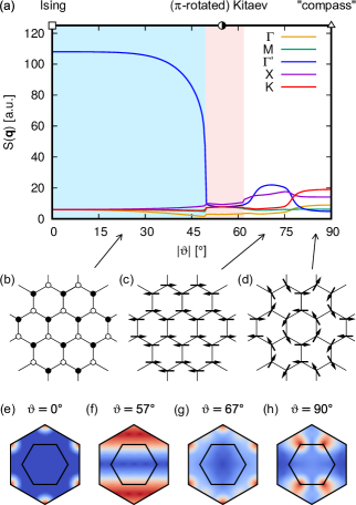
Figure 7: (a) Trace of the spin structure factor $S(\boldsymbol{q})=\sum_{\alpha}\langle S^{\alpha}_{-\boldsymbol{q}}S^{\alpha}_{\boldsymbol{q}}\rangle$ obtained by ED using hexagonal $24$-site cluster. The calculation reveals an Ising antiferromagnet and a Kitaev liquid phase; for high values of $|\vartheta|$ (interaction axis near the honeycomb plane), the correlations show a mixture of contributions mainly at $\Gamma^{\prime}$, X and K points. (b)-(d) Most probable spin configurations determined by the method of spin-$\tfrac{1}{2}$ coherent states (using $\varphi=\pi/2$). The Néel state is out of plane in (b) and only slightly tilted from the plane in (c). The spin arrangement (d) is the same as the vortex-$a$ configuration shown in Fig. 2(b). (e)-(h) Spin-spin correlations $\langle S^{z}_{-\boldsymbol{q}}S^{z}_{\boldsymbol{q}}\rangle$ for a few selected values of $\vartheta$ and $\varphi=\pi/2$. In panel (f), the typical cosine wave pattern characterizing a spin liquid state appears.

The resulting phase diagram is shown in Fig. 7. We formally plot it as function of $|\vartheta|$. For negative values of $\vartheta$ it covers the range Ising – $\pi$-rotated Kitaev – “compass” that is continuously visible in Fig. 6(e). The phase diagram for positive $\vartheta$ is identical, even though corresponding to different line in the parameter space of the EKH model.

More than half of the phase diagram is occupied by the AF Ising phase with the moments pointing in the $(111)$ direction. It starts as fluctuation free at the Ising point $\vartheta=0^{\circ}$ and gradually acquires more quantum fluctuating nature until $|\vartheta|\approx 49.5^{\circ}$ where a transition to a spin-liquid associated with the ($\pi$-rotated) Kitaev point at $|\vartheta|\approx 54.7^{\circ}$ happens. The increasing content of quantum fluctuations is manifested by decreasing spin correlations [Fig. 7(a)] or the probability of Néel state in the ground state which follows a similar curve. At approximately $62^{\circ}$ the spin liquid state breaks down. Compared to the tensor network study [100], we find a significantly wider spin liquid window – $(49.5^{\circ},62^{\circ})$ vs $(52.7^{\circ},57.6^{\circ})$. The reason for this discrepancy is not clear, an earlier tensor-network study of the Kitaev-Heisenberg model [85] was in a good agreement with ED. One possibility is that a different procedure of finding the level crossings or extrapolating the bond dimension has been used for the two tensor networks studies.

For $|\vartheta|\gtrsim 62^{\circ}$, the ground state is characterized by peaks in the structure factor at the $\Gamma^{\prime}$ and X point [see Fig. 7(g)], while around $|\vartheta|\approx 77^{\circ}$ the correlations at $\Gamma^{\prime}$ point drop and the K point becomes dominant [Fig. 7(h)]. In the first part of this interval, the method of spin-$\tfrac{1}{2}$ coherent states finds a Néel state with the moment direction slightly tilted ($\lesssim 5^{\circ}$) from the honeycomb plane [Fig. 7(c)] and the amount of quantum fluctuations comparable to the ground state of the AF Heisenberg model. After a transition at about $77^{\circ}$, a vortex-a pattern is found [Fig. 7(d)], but with a probability $P\approx 3\%$ significantly smaller than observed earlier inside the vortex phase. This suggests that the second phase might be possibly disordered, as claimed previously by [98] and [99] for the compass model. The absence of visible changes in the correlations in the region of the second phase indicates that the features of “compass” limit $|\vartheta|=90^{\circ}$ are kept throughout this phase. Similarly to the vortex phase, the most probable pattern (vortex-a) is accompanied by the complementary pattern (vortex-b) having a very close probability ($P\approx 3.16\%$ vs $3.05\%$ in the AF “compass” limit). The same pair but with the swapped probabilities is found for FM compass point discussed in Sec. VI.1. This is natural since the two models as well as the two patterns are linked by a simple $90^{\circ}$ rotation of the spins (interchanging the in-bond and perpendicular components), followed by a $180^{\circ}$ rotation at every second site (converting AF to FM and vice versa).

Finally, we note that the presence of two distinct phases between the spin liquid phase and the compass limit is at odds with the conclusion of Ref. [100] that the whole interval is occupied by a dimer phase. To check the reliability of our phase diagram, we have performed an additional ED for $32$-site clusters of two different shapes, confirming the existence of the Néel phase for those clusters as well.

VII Conclusions

We have performed a detailed numerical investigation of the global phase diagram of the extended Kitaev-Heisenberg model including the analysis of the internal structure of the individual phases. To this end, we have used mainly exact diagonalization combined with a recently developed ground-state analysis based on spin-$\frac{1}{2}$ coherent states.

In the context of real materials such as Na₂IrO₃ or $\alpha$-RuCl₃, our results are useful when judging the extent of the experimentally observed zigzag phase and comparing the direction of the ordered moments, fixing thereby the relevant window in the parameter space.

In more general terms, we have interpreted the trends in the phase diagram based on several types of symmetry features found in the extended Kitaev-Heisenberg model, providing a number of reference points of expected behavior. They include points of hidden SU(2) symmetry, manifolds of fluctuation-free ground states, and mappings to other models: Ising, compass, and hidden Kitaev model. We have demonstrated that while being in principle simple results of linear algebra, these symmetry features have far-reaching consequences and well fix the overall structure of the global phase diagram. As we believe, our symmetry-guided study can serve as a methodological template that can be applied to other spin models with bond-dependent non-Heisenberg interactions emerging in the field of Mott insulators with strong spin-orbit coupling.

Among the unusual symmetry properties brought about by the bond-dependent non-Heisenberg interactions, we have highlighted two interesting features that, to the best of our knowledge, escaped attention so far:
(i) Fluctuation-free ground states on entire manifolds of parameter points, possessing both FM and AF ordering patterns. These are enabled due to a partial cancellation of interactions for the particular spin structure. However, above the ground state, these interactions are fully active and shall lead to excitation spectra quite distinct from those of e.g. Heisenberg FM.
(ii) Models with bond-dependent non-Heisenberg interactions may realize not only the sought-after Kitaev model but also other models with a single bond-dependent interacting spin component (“interaction axis”). In the case of the extended Kitaev-Heisenberg model, they range from the simple Ising model, through Kitaev, to the $120^{\circ}$ compass model on honeycomb lattice, whose ground-state nature is still debated in the literature. The above models are continuously connected in the parameter space of the extended Kitaev-Heisenberg model and the corresponding line in the phase diagram contains both trivial (Ising limit) as well as highly nontrivial phases – perturbed Kitaev spin liquid and the phase associated with the perturbed compass model. Such links to the extended Kitaev-Heisenberg model may motivate a search for candidate materials realizing, e.g. a compass model.

Appendix A Optimized spin-$\frac{1}{2}$ coherent states in the presence of spin liquid phases

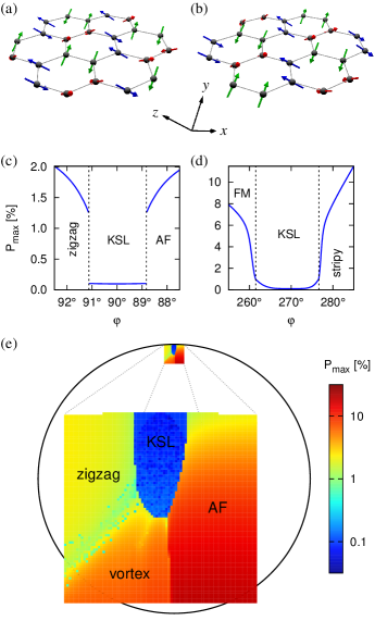
Figure 8: Most probable configurations near the (a) AF and (b) FM Kitaev point. Spins pointing along the $x$, $y$, and $z$ cubic axes are marked by red, green, and blue color, respectively. (c) Probability $P_{\mathrm{max}}$ of the optimized configuration near the AF Kitaev point in the Kitaev-Heisenberg model parametrized as $J=\cos\varphi$, $K=\sin\varphi$. Phase transitions to the neighboring ordered phases are indicated by dashed lines. (d) The same for the region around the FM Kitaev point. (e) Map of $P_{\mathrm{max}}$ in a small area near the AF Kitaev spin liquid phase in the extended Kitaev-Heisenberg model with $\Gamma^{\prime}=J_{3}=0$ (belongs to the same slice as shown in Fig. 2).

In contrast to the ordered phases, the ground states of Kitaev spin liquid (KSL) phases are highly entangled and cannot be well described by a spin-$\frac{1}{2}$ coherent state (4) that is a simple product of spin-$\frac{1}{2}$ states. This is indeed observed when applying the method of Sec. III.1 to the spin-liquid ground state. Nevertheless, the spin-liquid ground state still has a significant overlap with the configurations found in the classical $S\rightarrow\infty$ limit of the Kitaev model. Shown in Fig. 8(a),(b) are the most probable configurations found in the exact ground state of the 24-site cluster near the AF or FM Kitaev point, respectively. They are characterized by spins pointing along the cubic axes $x$, $y$, $z$ and forming aligned (FM case) or contra-aligned (AF case) pairs on nearest-neighbor bonds. Their orientation is determined by the bond direction which is linked to the active spin component in the Kitaev interaction.

It is instructive to inspect the evolution of probability $P_{\mathrm{max}}$ of the optimized spin-$\frac{1}{2}$ coherent state when going from the KSL phase through a quantum phase transition to the neighboring ordered phases. This is done in Fig. 8(c) for the case of AF Kitaev model perturbed by Heisenberg interaction. While the KSL is characterized by small $P_{\mathrm{max}}\approx 0.1\%$, at the phase boundary either to zigzag or to AF ordered phase $P_{\mathrm{max}}$ jumps by about one order of magnitude to values above $1\%$ typically encountered in the main text for the ordered phases with significant quantum fluctuations. A different behavior is found in the FM case. Here the probability rises near the phase boundaries to FM and stripy phases and continuously connects to $P_{\mathrm{max}}$ of their groundstates. However, a discontinuity still appears in the derivative with respect to model parameters, with $P_{\mathrm{max}}$ shooting up after crossing the phase boundary. This is yet another manifestation of the different nature of the phase transitions involving AF and FM KSL phases that shows up e.g. in the behavior of the spin-excitation gap [81].

Finally, in Fig. 8(e) we consider a larger portion of the phase diagram near the AF KSL phase which also involves the nonzero $\Gamma>0$ parameter case. The AF KSL phase can be easily distinguished again by a drop of $P_{\mathrm{max}}$. The case of FM KSL phase at the bottom of the corresponding phase diagram slice is more complicated by the less pronounced transition and more complex phase behavior in the surrounding region as discussed in Sec. IV.3. Fig. 8(e) also illustrates the difficulties of the global optimization in the complete 48-dimensional space of $\theta$ and $\phi$ parameters corresponding to the 24-site cluster. As seen in Fig. 8(e), the danger of getting trapped in a local maximum increases e.g. near the zigzag/vortex phase boundary or in the KSL phase characterized by competing configurations.

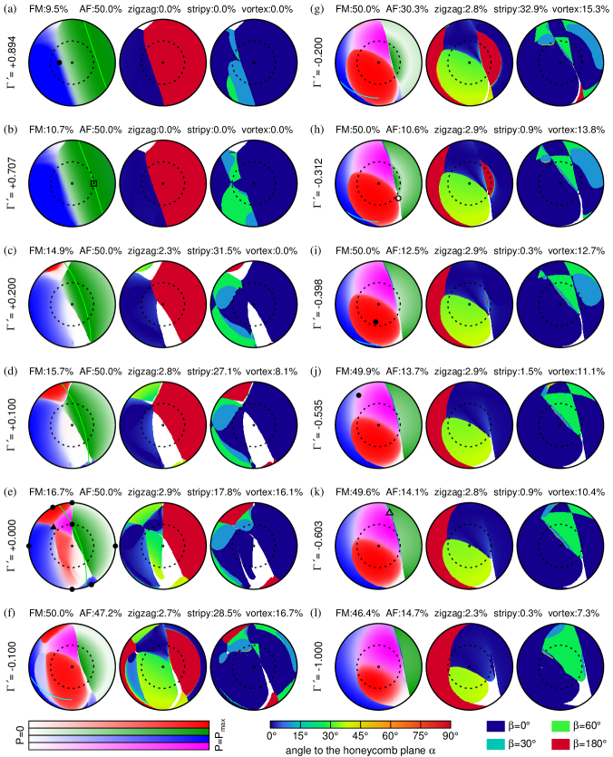
Figure 9: Phase diagram slices for selected $\Gamma^{\prime}$ values and $J_{3}=0$. Left circle in each panel shows a colormap of the probabilities of the patterns: FM (blue), AF (green), zigzag (red), stripy (blue), vortex (violet). The ranges of the corresponding scales (bottom left) are determined by the maximum probability $P_{\mathrm{max}}$ as given at the top of the individual panels. Middle circles show the angle to the honeycomb plane (common scale at bottom center). Right circles show the azimuthal angle $\varphi$ within the honeycomb plane. Fluctuation-free lines given by Eq. (13) (FM phase, light blue) and (16) (AF phase, light green) are indicated along with the special points: (hidden) SU(2) symmetry points [$\bullet$ in panels (a),(e),(i),(j)], Kitaev points [$\bullet$ in (e), $\circ$ in (h)], Ising point [$\Box$ in (b)], compass point [$\blacktriangle$ in (e)] and compass-like point [$\vartriangle$ in (k)].

Appendix B Ising-Kitaev-compass model – derivation

The EKH Hamiltonian has a single matrix form for all bond directions when written in the rotating reference frame $\tilde{x}_{\gamma},\tilde{y}_{\gamma},\tilde{z}_{\gamma}$:

$$\widetilde{H}=\begin{pmatrix}J-\Gamma&0&0\\[8.00003pt] 0&J+\tfrac{2K}{3}+\tfrac{\Gamma}{3}-\tfrac{4\Gamma^{\prime}}{3}&\tfrac{\sqrt{2}}{3}(K-\Gamma+\Gamma^{\prime})\\[8.00003pt] 0&\tfrac{\sqrt{2}}{3}(K-\Gamma+\Gamma^{\prime})&J+\tfrac{K}{3}+\tfrac{2\Gamma}{3}+\tfrac{4\Gamma^{\prime}}{3}\end{pmatrix}.$$ (26)

The matrix consists of two blocks, therefore one principal axis is $\tilde{x}_{\gamma}$ and the other two lie in the $\tilde{y}_{\gamma}\tilde{z}_{\gamma}$ plane. The eigenvalues of this matrix are:

$$\lambda_{1} =J-\Gamma,$$

$$\lambda_{2} =J+\tfrac{1}{2}(K+\Gamma+\sqrt{(K-\Gamma)^{2}+8\Gamma^{\prime 2}}),$$

$$\lambda_{3} =J+\tfrac{1}{2}(K+\Gamma-\sqrt{(K-\Gamma)^{2}+8\Gamma^{\prime 2}}).$$ (27)

If only the first eigenvalue $\lambda_{1}=J=\Gamma$ is non-zero, we obtain the 120^∘ honeycomb compass model, the situation discussed in Section VI.1. For $\Gamma>0$, one can find a parameter region where only $\lambda_{2}$ is non-zero:

$$J=\Gamma,\;J(J+K)=\Gamma^{\prime 2},\;J>0,\;J+K>0.$$ (28)

Analogous to this case, for $\Gamma<0$ only $\lambda_{3}$ is non-zero in the region given by

$$J=\Gamma,\;J(J+K)=\Gamma^{\prime 2},\;J<0,\;J+K<0.$$ (29)

The sole non-zero eigenvalue in both of these cases equals $3J+K$ and its sign is the same as the sign of $\Gamma$, hence in the case $\Gamma>0$ used in the main text $3J+K>0$ and the interaction is antiferromagnetic. The parameter region (28) [or (29)] can be parametrized by a single variable, which we choose as the angle $\vartheta$ between the $\tilde{z}_{\gamma}=Z$ axis and the interaction direction. In terms of the model parameters, $\vartheta$ is given by

$$\tan 2\vartheta=2\sqrt{2}\left(\frac{9\Gamma^{\prime}}{J-K+8\Gamma^{\prime}}-1\right).$$ (30)

It is also easy to obtain the parameters $J$, $K$, $\Gamma$, $\Gamma^{\prime}$ realizing the model (22) with arbitrary $\vartheta$ and $\varphi=\pi/2$:

$$J=\Gamma =\tilde{K}\,\tfrac{1}{6}\bigl{[}1+\cos\vartheta(\cos\vartheta-\sqrt{8}\sin\vartheta)\bigr{]},$$ (31)

$$K =\tilde{K}\,\tfrac{1}{2}\bigl{[}1-\cos\vartheta(\cos\vartheta-\sqrt{8}\sin\vartheta)\bigr{]},$$ (32)

$$\Gamma^{\prime} =\tilde{K}\,\tfrac{1}{3}\bigl{[}\cos 2\vartheta+\tfrac{1}{\sqrt{8}}\sin 2\vartheta)\bigr{]}.$$ (33)

Finally, as demonstrated in Ref. [75], the nearest-neighbor EKH model preserves its form under global rotation of the spin axes by $\pi$ around the $(111)$ direction. This transformation, labeled as $\mathcal{T}_{1}$ in Ref. [75], maps the model parameters $JK\Gamma\Gamma^{\prime}$ onto another set according to Eq. (4) of Ref. [75]. In the context of the Ising-Kitaev-compass model, the rotation by $\pi$ around $(111)$ axis corresponds to a sign change $\vartheta\rightarrow-\vartheta$. Indeed, inserting the transformed set of parameters into Eq. 30, one observes the sign change. Obviously, the $\mathcal{T}_{1}$ transformation does not have any effect in the Ising ($\vartheta=0$) and compass/“compass” ($\vartheta=\pm\pi/2$) case. Apart from these cases, it connects various pairs of points on the curves in Fig. 6(c)-(e), most importantly, the Kitaev model and its $\pi$-rotated variant.

Appendix C Detailed evolution of the phase diagram for nonzero $\Gamma^{\prime}$

Figure 9 presents a detailed evolution of the phases of the nearest neighbor model ($J_{3}=0$) with the parameter $\Gamma^{\prime}$ attaining both positive and negative values. It was obtained using the method of Sec. III.1 for the hexagon-shaped 24-site cluster. The $\Gamma^{\prime}$ values were selected to include all the special symmetry points discussed in Ref. [75] and in the present paper. The lines of fluctuation-free ground states discussed in Sec. V are also indicated.

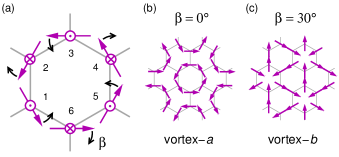
Figure 10: (a) Moment directions defined by Eq. (35) capturing vortex in-plane structure and out-of-plane AF staggering. For the in-plane deviation angle $\beta=0^{\circ}$ and $\beta=30^{\circ}$, we get the patterns (b) vortex-a and (c) vortex-b of Fig. 2(b), respectively.

The plots use the same parametrization of the interactions as that of Fig. 2 and show also the moment direction in the form of an angle to the honeycomb plane $\alpha$ and an azimuthal angle in the honeycomb plane $\beta$. Using the $XYZ$ reference frame of Fig. 5(b), the moment direction in the collinear phases is given by

$$\boldsymbol{n}=(\cos\alpha\cos\beta,\cos\alpha\sin\beta,\sin\alpha).$$ (34)

For the moments lying in the honeycomb plane, $\beta=0^{\circ}$ corresponds to the direction perpendicular to a bond while $\beta=30^{\circ}$ is in-bond direction. The values $\beta=60^{\circ}$ and $\beta=180^{\circ}$ are used in the out-of-plane cases where a further distinction is necessary. In the vortex phase, the directions of the moments at the six sublattices marked in Fig. 5(c) are

$$\boldsymbol{n}_{k}=\bigl{(}\,\cos\alpha\cos\beta_{k},\cos\alpha\sin\beta_{k},(-1)^{k-1}\sin\alpha\,\bigr{)},$$ (35)

where $\beta_{k}=(-1)^{k-1}\beta-60^{\circ}k$ and $k=1,2,\ldots 6$ labels the sublattice. This Ansatz, depicted in Fig. 10, captures both patterns vortex-a ($\beta=0^{\circ}$ or $\beta=60^{\circ}$) and vortex-b ($\beta=30^{\circ}$) shown in Fig. 2(b) and AF staggering in the direction perpendicular to the honeycomb plane (nonzero $\alpha$).

Not indicated in Fig. 9 are the regions of the instability of the zigzag phase observed in Fig. 2(a) and Fig. 4(a),(b). Apart from the ones shown earlier, the regions with non-collinear tendencies appear for large negative $\Gamma^{\prime}\lesssim-0.5$ near the meeting point of the zigzag phase with FM and vortex phases and, to a smaller extent, also at the bottom near the white region in Fig. 9(j)-(l). Since the smaller zigzag phase visible in Fig. 9(c)-(f) is a copy of the larger zigzag phase linked by the exact $\mathcal{T}_{1}$ transformation, it also contains such patches of instability. Similarly, the top and bottom white areas hosting incommensurate orderings [visible in Fig. 9(a)-(c) and Fig. 9(c)-(f), respectively] are linked by the $\mathcal{T}_{1}$ transformation. The white area of Fig. 9(j)-(l) maps to the $\Gamma<0$ case.

References

- [1] C. Lacroix, P. Mendels, and F. Mila (Eds.), Introduction to Frustrated Magnetism (Springer, Berlin, 2011).
- [2] L. Balents, Nature 464, 199208 (2010).
- [3] L. Savary and L. Balents, Rep. Prog. Phys. 80, 016502 (2017).
- [4] S. T. Bramwell and M. J. P. Gingras, Science 294, 14951501 (2001).
- [5] C. Castelnovo, R. Moessner, and S. L. Sondhi, Annu. Rev. Condens. Matter Phys. 3, 35 (2012).
- [6] M. R. Norman, Rev. Mod. Phys. 88, 041002 (2016).
- [7] P. Chandra and B. Doucot, Phys. Rev. B 38, 9335 (1988).
- [8] S. Chakravarty, B. I. Halperin, and D. R. Nelson, Phys. Rev. B 39, 2344 (1989).
- [9] B. Schmidt and P. Thalmeier, Phys. Rep. 703, 1 (2017).
- [10] W. Witczak-Krempa, G. Chen, Y. B. Kim, and L. Balents, Annu. Rev. Condens. Matter Phys. 5, 57 (2014).
- [11] Z. Nussinov and J. van den Brink, Rev. Mod. Phys. 87, 159 (2015).
- [12] J. G. Rau, E. K.-H. Lee, and H.-Y. Kee, Annu. Rev. Condens. Matter Phys. 7, 195 (2016).
- [13] R. Schaffer, E. K.-H. Lee, B.-J. Yang, and Y. B. Kim, Rep. Prog. Phys. 79, 094504 (2016).
- [14] S. Trebst, arXiv:1701.07056 [cond-mat.str-el].
- [15] S. M. Winter, A. A. Tsirlin, M. Daghofer, J. van den Brink, Y. Singh, P. Gegenwart, and R. Valentí, J. Phys.: Condens. Matter 29, 493002 (2017).
- [16] M. Hermanns, I. Kimchi, and J. Knolle, Annu. Rev. Condens. Matter Phys. 9, 17 (2018).
- [17] A. Kitaev, Ann. Phys. 321, 2 (2006).
- [18] A. Abragam and B. Bleaney, Electron Paramagnetic Resonance of Transition Ions (Clarendon Press, Oxford, 1970).
- [19] G. Khaliullin, Prog. Theor. Phys. Suppl. 160, 155 (2005).
- [20] B. J. Kim, H. Jin, S. J. Moon, J.-Y. Kim, B.-G. Park, C. S. Leem, J. Yu, T. W. Noh, C. Kim, S.-J. Oh, J.-H. Park, V. Durairaj, G. Cao, and E. Rotenberg, Phys. Rev. Lett. 101, 076402 (2008).
- [21] B. J. Kim, H. Ohsumi, T. Komesu, S. Sakai, T. Morita, H. Takagi, and T. Arima, Science 323, 1329 (2009).
- [22] G. Jackeli and G. Khaliullin, Phys. Rev. Lett. 102, 017205 (2009).
- [23] J. Kim, D. Casa, M. H. Upton, T. Gog, Y.-J. Kim, J. F. Mitchell, M. van Veenendaal, M. Daghofer, J. van den Brink, G. Khaliullin, and B. J. Kim, Phys. Rev. Lett. 108, 177003 (2012).
- [24] Y. K. Kim, O. Krupin, J. D. Denlinger, A. Bostwick, E. Rotenberg, Q. Zhao, J. F. Mitchell, J. W. Allen, and B. J. Kim, Science 345, 187 (2014).
- [25] Y. K. Kim, N. H. Sung, J. D. Denlinger, and B. J. Kim, Nat. Phys. 12, 37 (2016).
- [26] K. I. Kugel and D. I. Khomskii, Sov. Phys. Usp. 25, 231 (1982).
- [27] G. Chen and L. Balents, Phys. Rev. B 78, 094403 (2008).
- [28] K. W. Plumb, J. P. Clancy, L. J. Sandilands, V. V. Shankar, Y. F. Hu, K. S. Burch, H.-Y. Kee, and Y.-J. Kim, Phys. Rev. B 90, 041112(R) (2014).
- [29] A. Banerjee, C. A. Bridges, J.-Q. Yan, A. A. Aczel, L. Li, M. B. Stone, G. E. Granroth, M. D. Lumsden, Y. Yiu, J. Knolle, S. Bhattacharjee, D. L. Kovrizhin, R. Moessner, D. A. Tennant, D. G. Mandrus, and S. E. Nagler, Nature Materials 15, 733 (2016).
- [30] K. Ran, J. Wang, W. Wang, Z.-Y. Dong, X. Ren, S. Bao, S. Li, Z. Ma, Y. Gan, Y. Zhang, J. T. Park, G. Deng, S. Danilkin, S.-L. Yu, J.-X. Li, and J. Wen, Phys. Rev. Lett. 118, 107203 (2017).
- [31] A. Banerjee, J. Yan, J. Knolle, C. A. Bridges, M. B. Stone, M. D. Lumsden, D. G. Mandrus, D. A. Tennant, R. Moessner, and S. E. Nagler, Science 356, 1055 (2017).
- [32] S.-H. Do, S.-Y. Park, J. Yoshitake, J. Nasu, Y. Motome, Y. S. Kwon, D. T. Adroja, D. J. Voneshen, K. Kim, T.-H. Jang, J.-H. Park, K.-Y. Choi, and S. Ji, Nature Phys. 13, 1079 (2017).
- [33] X. Liu, T. Berlijn, W.-G. Yin, W. Ku, A. Tsvelik, Y.-J. Kim, H. Gretarsson, Y. Singh, P. Gegenwart, and J. P. Hill, Phys. Rev. B 83, 220403(R) (2011).
- [34] F. Ye, S. Chi, H. Cao, B. C. Chakoumakos, J. A. Fernandez-Baca, R. Custelcean, T. F. Qi, O. B. Korneta, and G. Cao, Phys. Rev. B 85, 180403(R) (2012).
- [35] S. K. Choi, R. Coldea, A. N. Kolmogorov, T. Lancaster, I. I. Mazin, S. J. Blundell, P. G. Radaelli, Y. Singh, P. Gegenwart, K. R. Choi, S.-W. Cheong, P. J. Baker, C. Stock, and J. Taylor, Phys. Rev. Lett. 108, 127204 (2012).
- [36] R. D. Johnson, S. C. Williams, A. A. Haghighirad, J. Singleton, V. Zapf, P. Manuel, I. I. Mazin, Y. Li, H. O. Jeschke, R. Valentí, and R. Coldea, Phys. Rev. B 92, 235119 (2015).
- [37] J. A. Sears, M. Songvilay, K. W. Plumb, J. P. Clancy, Y. Qiu, Y. Zhao, D. Parshall, and Y.-J. Kim, Phys. Rev. B 91, 144420 (2015).
- [38] S. C. Williams, R. D. Johnson, F. Freund, S. Choi, A. Jesche, I. Kimchi, S. Manni, A. Bombardi, P. Manuel, P. Gegenwart, and R. Coldea, Phys. Rev. B 93, 195158 (2016).
- [39] K. Kitagawa, T. Takayama, Y. Matsumoto, A. Kato, R. Takano, Y. Kishimoto, S. Bette, R. Dinnebier, G. Jackeli, and H. Takagi, Nature 554, 341345 (2018).
- [40] J. Chaloupka, G. Jackeli, and G. Khaliullin, Phys. Rev. Lett. 110, 097204 (2013).
- [41] S. H. Chun, J.-W. Kim, Jungho Kim, H. Zheng, C. C. Stoumpos, C. D. Malliakas, J. F. Mitchell, K. Mehlawat, Y. Singh, Y. Choi, T. Gog, A. Al-Zein, M. Moretti Sala, M. Krisch, J. Chaloupka, G. Jackeli, G. Khaliullin, and B. J. Kim, Nature Phys. 11, 462 (2015).
- [42] J. G. Rau, E. K.-H. Lee, and H.-Y. Kee, Phys. Rev. Lett. 112, 077204 (2014).
- [43] J. G. Rau and H.-Y. Kee, ArXiv e-prints (2014), arXiv:1408.4811 [cond-mat.str-el].
- [44] V. M. Katukuri, S. Nishimoto, V. Yushankhai, A. Stoyanova, H. Kandpal, S. Choi, R. Coldea, I. Rousochatzakis, L. Hozoi, and J. van den Brink, New J. Phys. 16, 013056 (2014).
- [45] Y. Yamaji, Y. Nomura, M. Kurita, R. Arita, and M. Imada, Phys. Rev. Lett. 113, 107201 (2014).
- [46] Y. Sizyuk, C. Price, P. Wölfle, and N. B. Perkins, Phys. Rev. B 90, 155126 (2014).
- [47] S. M. Winter, Y. Li, H. O. Jeschke, and R. Valentí, Phys. Rev. B 93, 214431 (2016).
- [48] S. M. Winter, K. Riedl, P. A. Maksimov, A. L. Chernyshev, A. Honecker, and R. Valentí, Nature Comm. 8, 1152 (2017).
- [49] P. A. McClarty, X.-Y. Dong, M. Gohlke, J. G. Rau, F. Pollmann, R. Moessner, and K. Penc, Phys. Rev. B 98, 060404(R) (2018).
- [50] D. G. Joshi, Phys. Rev. B 98, 060405(R) (2018).
- [51] M. Becker, M. Hermanns, B. Bauer, M. Garst, and S. Trebst, Phys. Rev. B 91, 155135 (2015).
- [52] I. Rousochatzakis, U. K. Rössler, J. van den Brink, and M. Daghofer, Phys. Rev. B 93, 104417 (2016).
- [53] K. Li, S.-L. Yu, and J.-X. Li, New J. Phys 17, 043032 (2015).
- [54] A. Catuneanu, J. G. Rau, H.-S. Kim, and H.-Y. Kee, Phys. Rev. B 92, 165108 (2015).
- [55] K. Morita, M. Kishimoto, and T. Tohyama, Phys. Rev. B 98, 134437 (2018).
- [56] T. Takayama, A. Kato, R. Dinnebier, J. Nuss, H. Kono, L. S. I. Veiga, G. Fabbris, D. Haskel, and H. Takagi, Phys. Rev. Lett. 114, 077202 (2015).
- [57] E. K-H. Lee and Y. B. Kim, Phys. Rev. B 91, 064407 (2015).
- [58] H.-S. Kim, E. K.-H. Lee, and Y. B. Kim, EPL 112, 67004 (2015).
- [59] E. K.-H. Lee, J. G. Rau and, Y. B. Kim, Phys. Rev. B 93, 184420 (2016).
- [60] V. M. Katukuri, R. Yadav, L. Hozoi, S. Nishimoto, and J. van den Brink, Sci. Rep. 6, 29585 (2016).
- [61] K. A. Modic, T. E. Smidt, I. Kimchi, N. P. Breznay, A. Biffin, S. Choi, R. D. Johnson, R. Coldea, P. Watkins-Curry, G. T. McCandless, J. Y. Chan, F. Gandara, Z. Islam, A. Vishwanath, A. Shekhter, R. D. McDonald, and J. G. Analytis, Nat. Comm. 5, 4203 (2014).
- [62] A. Biffin, R. D. Johnson, I. Kimchi, R. Morris, A. Bombardi, J. G. Analytis, A. Vishwanath, and R. Coldea, Phys. Rev. Lett. 113, 197201 (2014).
- [63] I. Kimchi, J. G. Analytis, and A. Vishwanath, Phys. Rev. B 90, 205126 (2014).
- [64] Y. Okamoto, M. Nohara, H. Aruga-Katori, and H. Takagi, Phys. Rev. Lett. 99, 137207 (2007).
- [65] G. Cao, A. Subedi, S. Calder, J.-Q. Yan, J. Yi, Z. Gai, L. Poudel, D. J. Singh, M. D. Lumsden, A. D. Christianson, B. C. Sales, and D. Mandrus, Phys. Rev. B 87, 155136 (2013).
- [66] A. M. Cook, S. Matern, C. Hickey, A. A. Aczel, and A. Paramekanti, Phys. Rev. B 92, 020417(R) (2015).
- [67] A. A. Aczel, A. M. Cook, T. J. Williams, S. Calder, A. D. Christianson, G.-X. Cao, D. Mandrus, Y.-B. Kim, and A. Paramekanti, Phys. Rev. B 93, 214426 (2016).
- [68] H. Kuriyama, J. Matsuno, S. Niitaka, M. Uchida, D. Hashizume, A. Nakao, K. Sugimoto, H. Ohsumi, M. Takata, and H. Takagi, Appl. Phys. Lett. 96, 182103 (2010).
- [69] I. Kimchi and A. Vishwanath, Phys. Rev. B 89, 014414 (2014).
- [70] M. Hermanns and S. Trebst, Phys. Rev. B 89, 235102 (2014).
- [71] H. Liu and G. Khaliullin, Phys. Rev. B 97, 014407 (2018).
- [72] R. Sano, Y. Kato, and Y. Motome, Phys. Rev. B 97, 014408 (2018).
- [73] J. M. Luttinger and L. Tisza, Phys. Rev. 70, 954 (1946).
- [74] J. Chaloupka, G. Jackeli, and G. Khaliullin, Phys. Rev. Lett. 105, 027204 (2010).
- [75] J. Chaloupka and G. Khaliullin, Phys. Rev. B 92, 024413 (2015).
- [76] L. Janssen, E. C. Andrade, and M. Vojta, Phys. Rev. B 96, 064430 (2017).
- [77] J. Lou, L. Liang, Y. Yu, and Y. Chen, ArXiv e-prints (2015), arXiv:1501.06990 [cond-mat.str-el].
- [78] K. Shinjo, S. Sota, and T. Tohyama, Phys. Rev. B 91, 054401 (2015).
- [79] S. Nishimoto, V. M. Katukuri, V. Yushankhai, H. Stoll, U. K. Rössler, L. Hozoi, I. Rousochatzakis, and J. van den Brink, Nat. Comm. 7, 10273 (2016).
- [80] J. Chaloupka and G. Khaliullin, Phys. Rev. B 94, 064435 (2016).
- [81] D. Gotfryd, J. Rusnačko, K. Wohlfeld, G. Jackeli, J. Chaloupka, and A. M. Oleś, Phys. Rev. B 95, 024426 (2017).
- [82] C. C. Price and N. B. Perkins, Phys. Rev. Lett. 109, 187201 (2012).
- [83] R. Schaffer, S. Bhattacharjee, and Y. B. Kim, Phys. Rev. B 86, 224417 (2012).
- [84] J. Reuther, R. Thomale, and S. Trebst, Phys. Rev. B 84, 100406(R) (2011).
- [85] J. O. Iregui, P. Corboz, and M. Troyer, Phys. Rev. B 90, 195102 (2014).
- [86] M. Gohlke, R. Verresen, R. Moessner, and F. Pollmann, Phys. Rev. Lett. 119, 157203 (2017).
- [87] F. Trousselet, M. Berciu, A. M. Oleś, and P. Horsch, Phys. Rev. Lett. 111, 037205 (2013).
- [88] F. Trousselet, P. Horsch, A. M. Oleś, and W.-L. You, Phys. Rev. B 90, 024404 (2014).
- [89] A. Avella and F. Mancini (Eds.), Strongly Correlated Systems: Numerical Methods (Springer, Berlin, 2013).
- [90] For a discussion of the order-from-disorder phenomena in frustrated spin systems, see A. M. Tsvelik, Quantum Field Theory in Condensed Matter Physics (Cambridge University Press, Cambridge, 1995), Chap. 17, and references therein.
- [91] G. Baskaran, D. Sen, and R. Shankar, Phys. Rev. B 78, 115116 (2008).
- [92] I. Rousochatzakis, Y. Sizyuk, and N. B. Perkins, Nat. Comm. 9, 1575 (2018).
- [93] M. Gohlke, G. Wachtel, Y. Yamaji, F. Pollmann, and Y. B. Kim, Phys. Rev. B 97, 075126 (2018).
- [94] P. P. Stavropoulos, A. Catuneanu, and H.-Y. Kee, Phys. Rev. B 98, 104401 (2018).
- [95] E. Quinn, S. Bhattacharjee, and R. Moessner, Phys. Rev. B 91, 134419 (2015).
- [96] E. Zhao and W. V. Liu, Phys. Rev. Lett. 100, 160403 (2008).
- [97] C. Wu, Phys. Rev. Lett. 100, 200406 (2008).
- [98] J. Nasu, A. Nagano, M. Naka, and S. Ishihara, Phys. Rev. B 78, 024416 (2008).
- [99] C.-C. Chen, L. Muechler, R. Car, T. Neupert, and J. Maciejko, Phys. Rev. Lett. 117, 096405 (2016).
- [100] H. Zou, B. Liu, E. Zhao, and W. V. Liu, New J. Phys. 18, 053040 (2016).