Robust Asset Allocation for Robo-Advisors

Abstract

In the last few years, the financial advisory industry has been impacted by the emergence of digitalization and robo-advisors. This phenomenon affects major financial services, including wealth management, employee savings plans, asset managers, private banks, pension funds, banking services, etc. Since the robo-advisory model is in its early stages, we estimate that robo-advisors will help to manage around $1 trillion of assets in 2020 (OECD, 2017). And this trend is not going to stop with future generations, who will live in a technology-driven and social media-based world.

In the investment industry, robo-advisors face different challenges: client profiling, customization, asset pooling, liability constraints, etc. In its primary sense, robo-advisory is a term for defining automated portfolio management. This includes automated trading and rebalancing, but also automated portfolio allocation. And this last issue is certainly the most important challenge for robo-advisory over the next five years. Today, in many robo-advisors, asset allocation is rather human-based and very far from being computer-based. The reason is that portfolio optimization is a very difficult task, and can lead to optimized mathematical solutions that are not optimal from a financial point of view (Michaud, 1989). The big challenge for robo-advisors is therefore to be able to optimize and rebalance hundreds of optimal portfolios without human intervention.

In this paper, we show that the mean-variance optimization approach is mainly driven by arbitrage factors that are related to the concept of hedging portfolios. This is why regularization and sparsity are necessary to define robust asset allocation. However, this mathematical framework is more complex and requires understanding how norm penalties impacts portfolio optimization. From a numerical point of view, it also requires the implementation of non-traditional algorithms based on ADMM methods and proximal operators.

Keywords: Robo-advisor, asset allocation, active management, portfolio optimization, Black-Litterman model, spectral filtering, machine learning, Tikhonov regularization, mixed penalty, ridge regression, lasso method, sparsity, ADMM algorithm, proximal operator.

JEL classification: C61, C63, G11.

1 Introduction

The concept of portfolio optimization has a long history and dates back to the seminal work of Markowitz (1952). In this paper, Markowitz defined precisely what portfolio selection means: “the investor does (or should) consider expected return a desirable thing and variance of return an undesirable thing”. This was the starting point of mean-variance optimization and portfolio allocation based on quantitative models. In particular, the Markowitz approach became the standard model for strategic asset allocation until the end of the 2000s.

Since the financial crisis of 2008, another model has emerged and is now a very serious contender for asset allocation (Roncalli, 2013). The risk budgeting approach is successfully used for managing multi-asset portfolios, equity risk factors or alternative risk premia. The main difference with mean-variance optimization is the objective function. The Markowitz approach mainly focuses on expected returns and exploits the trade-off between performance and volatility. The risk budgeting approach is based on the risk allocation of the portfolio, and does not take into account expected returns of assets.

The advantage of the risk budgeting approach is that it produces stable and robust portfolios. On the contrary, mean-variance optimization is very sensitive to input parameters. These stability issues make the practice of portfolio optimization less attractive than the theory (Michaud, 1989). Even for strategic asset allocation, many weight constraints need to be introduced in order to regularize the mathematical solution and obtain an acceptable financial solution. In the case of tactical asset allocation, professionals generally prefer to implement the model of Black and Litterman (1991, 1992), because the optimized portfolio depends on the current allocation. Therefore, the Black-Litterman model appears to be slightly more robust than the Markowitz model because having a benchmark or introducing a tracking error constraint is already a form of portfolio regularization. However, since the Black-Litterman model is a slight modification of the Markowitz model, it suffers from the same drawbacks.

Since the 1990s, academics have explored how to robustify portfolio optimization in two different directions. The first one deals with the estimation of the input parameters. For instance, we can use de-noising methods (Laloux et al., 1999) or shrinkage approaches (Ledoit and Wolf, 2004) to reduce estimation errors of the covariance matrix. The second one deals with the objective function. As explained by Roncalli (2013), the Markowitz model is an aggressive model of active management due to the mean-variance objective function. Academics have suggested regularizing the optimization problem by adding penalization functions. For instance, it is common to include a $L_{1}$ or $L_{2}$ norm loss function. The advantage of this is to obtain a “sparser” or “smoother” solution.

The success of risk parity, equal risk contribution (ERC) and risk budgeting portfolios has put these new developments in second place. However, the rise of robo-advisors is changing the current trend and highlights the need for active allocation models that are focused on expected returns. Indeed, the challenge of robo-advice concerns tactical asset allocation and not the portfolio construction of strategic asset allocation. Building a defensive, balance or dynamic portfolio profile is not an issue, because they are defined from an ex-ante point of view. Quantitative models can be used to define this step, but they are not necessarily required. For example, this step can also be done using a discretionary approach, since portfolio profiles are revised once and for all. The difficulty lies with the life of the invested portfolio and the dynamic allocation. A robo-advisor that would consist in rebalancing a constant-mix allocation is not a true robo-advisor, since it is reduced to the profiling of clients. The main advantage of robo-advisors is to perform dynamic allocation by including investment views, side assets or the client’s dynamic constraints, or some alpha engines provided by the robo-advisor’s manager or distributor.

The challenge for a robo-advisor is therefore to perform dynamic allocation or tactical asset allocation in a systematic way without human interventions. In this case, expected returns or trading signals must be taken into account. One idea is to consider an extension of the ERC portfolio by using a risk measure that depends on expected returns (Roncalli, 2015). However, this approach is not always suitable when we target a high tracking error. Otherwise, it makes a lot of sense for the mean-variance optimization to be the allocation engine of robo-advisors. As said previously, the challenge is to develop a robust asset allocation model. The purpose of this research is to provide a practical solution that does not require human interventions.

This paper is organized as follows. Section Two illustrates the practice of mean-variance optimization and highlights the limits of such models. In Section Three, we apply the theory of regularization to asset allocation. In particular, we point out the calibration procedure of the Lagrange coefficients of norm functions. In Section Four, we consider application to robo-advisory. Finally, Section Five offers some concluding remarks.

2 Practice and limits of mean-variance optimization

2.1 The mean-variance optimization framework

We follow the presentation of Roncalli (2013). We consider a universe of $n$ assets. Let $x=\left(x_{1},\ldots,x_{n}\right)$ be the vector of weights in the portfolio. We denote by $\mu$ and $\Sigma$ the vector of expected returns and the covariance matrix of asset returns. It follows that the expected return and the volatility of the portfolio are equal to $\mu\left(x\right)=x^{\top}\mu$ and $\sigma\left(x\right)=\sqrt{x^{\top}\Sigma x}$. The Markowitz approach consists in maximizing the expected return of the portfolio under a volatility constraint ($\sigma$-problem):

$$x^{\star}=\arg\max\mu\left(x\right)\text{ s.t. }\sigma\left(x\right)\leqslant\sigma^{\star}$$ (1)

or minimizing the volatility of the portfolio under a return constraint ($\mu$-problem):

$$x^{\star}=\arg\min\sigma\left(x\right)\text{ s.t. }\mu\left(x\right)\geqslant\mu^{\star}$$ (2)

Replacing the volatility by the variance scaled with the factor $\nicefrac{{1}}{{2}}$ does not change the solution. Therefore, we deduce that the Lagrange functions associated with Problems (1) and (2) are:

$$\mathcal{L}_{1}\left(x,\lambda_{1},\sigma^{\star}\right)=x^{\top}\mu-\lambda_{1}\left(\frac{1}{2}\sigma^{2}\left(x\right)-\frac{1}{2}\sigma^{\star^{2}}\right)$$

and:

$$\mathcal{L}_{2}\left(x,\lambda_{2},\mu^{\star}\right)=\frac{1}{2}\sigma^{2}\left(x\right)-\lambda_{2}\left(\mu\left(x\right)-\mu^{\star}\right)$$

They satisfy $\mathcal{L}_{2}\left(x,\lambda_{2},0\right)=-\lambda_{2}\mathcal{L}_{1}\left(x,\theta,0\right)$ where $\theta=\lambda_{2}^{-1}$ is the risk aversion of the quadratic utility function. As strong duality holds, these two problems are equivalent. Moreover, we can show that they can be written as a standard quadratic programming problem (Markowitz, 1956):

$$x^{\star}\left(\gamma\right)=\arg\min\frac{1}{2}x^{\top}\Sigma x-\gamma x^{\top}\mu$$ (3)

where $\gamma$ is the risk/return trade-off parameter. Since the problem is strongly convex and the solution is $x^{\star}\left(\gamma\right)=\gamma\Sigma^{-1}\mu$, we deduce that the solution of the $\mu$-problem is given by:

$$\gamma=\frac{\mu^{\star}}{\mu^{\top}\Sigma^{-1}\mu}$$

whereas the solution of the $\sigma$-problem is obtained for the following value of $\gamma$:

$$\gamma=\frac{\sigma^{\star}}{\sqrt{\mu^{\top}\Sigma^{-1}\mu}}$$

The previous framework can be extended by considering a risk-free asset and portfolio constraints:

$$x^{\star}\left(\gamma\right) = \arg\min\frac{1}{2}x^{\top}\Sigma x-\gamma x^{\top}\left(\mu-r\mathbf{1}\right)$$

s.t. $$x\in\Omega$$

where $r$ is the risk-free rate and $\Omega$ is the set of restrictions. Let $\mu^{-}\leqslant\mu\left(x\right)\leqslant\mu^{+}$ and $\sigma^{-}\leqslant\sigma\left(x\right)\leqslant\sigma^{+}$ be the bounds of the expected return and the volatility such that $x\in\Omega$. It follows that there is a solution to the $\sigma$-problem and the $\mu$-problem if $\sigma^{\star}\geqslant\sigma^{-}$ and $\mu^{\star}\leqslant\mu^{+}$.

Remark 1

The Sharpe ratio is the standard risk/return measure used in finance, and corresponds to the zero-homogeneous quantity:

$$\mathop{\rm SR}\left(x\mid r\right) = \frac{\mu\left(x\right)-r}{\sigma\left(x\right)}$$

$$= \frac{x^{\top}\mu-r}{\sqrt{x^{\top}\Sigma x}}$$

The capital asset pricing model (CAPM) defines the tangency portfolio as the optimized portfolio that has the maximum Sharpe ratio. When the capital budget is reached (meaning that $\sum_{i=1}^{n}x_{i}=1$), the solution of Problem (2.1) is equal to $x^{\star}=\gamma\Sigma^{-1}\left(\mu-r\mathbf{1}\right)$ where $\gamma^{\star}=\left(\mathbf{1}^{\top}\Sigma^{-1}\left(\mu-r\mathbf{1}\right)\right)^{-1}$. Since the matrix $\Sigma$ has a unique symmetric positive definite square root denoted by $\Sigma^{1/2}$, the Cauchy-Schwarz inequality yields:

$$\left(x^{\top}\left(\mu-r\mathbf{1}\right)\right)^{2}=\left(x^{\top}\Sigma^{1/2}\Sigma^{-1/2}\left(\mu-r\mathbf{1}\right)\right)^{2}\leqslant\left(x^{\top}\Sigma x\right)\left(\left(\mu-r\mathbf{1}\right)^{\top}\Sigma^{-1}\left(\mu-r\mathbf{1}\right)\right)$$

The equality holds if and only if there exists a scalar $\gamma\in\mathbb{R}$ such that $\Sigma^{1/2}x=\gamma\Sigma^{-1/2}\left(\mu-r\mathbf{1}\right)$. It follows that:

$$\forall\,x\in\mathbb{R}^{n}\quad\mathop{\rm SR}\left(x\mid r\right)\leqslant\sqrt{\left(\mu-r\mathbf{1}\right)^{\top}\Sigma^{-1}\left(\mu-r\mathbf{1}\right)}$$ (5)

We deduce that the set of portfolios maximizing the Sharpe ratio is the one-dimensional vector space defined by $x\in\Sigma^{-1}\left(\mu-r\mathbf{1}\right)$. This means that unconstrained and constrained portfolio optimizations are related when we impose only one simple constraint like the capital budget restriction. In more complex cases, the constrained solution is not necessarily related to the unconstrained solution. However, the bound remains valid, because it only depends on the Cauchy-Schwarz inequality.

The previous result highlights the importance of constraints in portfolio optimization. A portfolio is long-only if $\forall\,i\in\{1,\ldots,n\}\ x_{i}\geqslant 0$ whereas it is long-short if $\exists\,\left(i,j\right)\in\{1,\ldots,n\}$ such that $x_{i}>0$ and $x_{j}<0$. For long-only portfolios, a capital budget is usually assumed, meaning that the portfolio is fully invested ($\sum_{i=1}^{n}x_{i}=1$). For long-short portfolios, professionals sometimes impose a neutral or zero-capital budget, implying that the long exposure is financed by the short exposure ($\sum_{i=1}^{n}x_{i}=0$). They can also impose leverage constraints ($\sum_{i=1}^{n}\left|x_{i}\right|\leqslant c$), while risk-budgeting portfolios require adding a logarithmic barrier constraint ($\sum_{i=1}^{n}\omega_{i}\ln x_{i}\geqslant c$).

In practice, the quantities $\mu$ and $\Sigma$ are unknown and must be specified. We can assume that they are estimated using an historical sample $\left\{R_{1},\ldots,R_{T}\right\}$ where $R_{t}$ is the vector of asset returns at time $t$. Let $\hat{\mu}$ and $\hat{\Sigma}$ be the corresponding estimators. We have:

$$\hat{\mu}=\sum_{t=1}^{T}w_{t}R_{t}$$

and:

$$\hat{\Sigma}=\sum_{t=1}^{T}w_{t}\left(R_{t}-\hat{\mu}\right)\left(R_{t}-\hat{\mu}\right)^{\top}$$

where $w_{t}$ is the weighting scheme such that $\sum_{t=1}^{T}w_{t}=1$. In Appendix A.2 on page A.2, we show that Problem (2.1) can be written as follows:

$$x^{\star}\left(\gamma\right) = \arg\min\frac{1}{2}\left\|Rx\right\|_{W}^{2}-\gamma x^{\top}\left(R^{\top}w-r\mathbf{1}\right)$$

s.t. $$x\in\Omega$$

where $w=\left(w_{1},\ldots,w_{T}\right)\in\mathbb{R}^{T}$, $R=\left(R_{1},\ldots,R_{T}\right)\in\mathbb{R}^{T\times n}$ and $W=\mathop{\rm diag}\left(w\right)-ww^{\top}$. In this case, the Markowitz solution is the portfolio that maximizes the backtest for a given volatility. When $w_{t+1}\geqslant w_{t}$, we conclude that Problem (2.1) is a trend-following optimization program, whose moving average is defined by the weighting scheme $w$. In order not to be trend-following, we have to use a vector of expected returns $\mu$ that does not satisfy $w_{t+1}\geqslant w_{t}$ or that does not depend on the sample of asset returns.

2.2 Stability issues

According to Hadamard (1902), a well-posed problem must satisfy three properties:

1. a solution exists;

2. the solution is unique;

3. the solution’s behavior changes continuously with the initial conditions.

We recall that the solution to Problem (3) is $x^{\star}\left(\gamma\right)=\gamma\Sigma^{-1}\mu$. If $\Sigma$ has no zero eigenvalues, it follows that the existence and uniqueness is ensured, but not necessarily the stability. Indeed, this third property implies that $\Sigma$ has no “small” eigenvalues. This problem is extensively illustrated by Bruder et al. (2013) and Roncalli (2013). If we consider the eigendecomposition $\Sigma=V\Lambda V^{\top}$, we have $\Sigma^{-1}=V\Lambda^{-1}V^{\top}$ and $x^{\star}\left(\gamma\right)=\gamma V\Lambda^{-1}V^{\top}\mu$. It follows that $V^{\top}x^{\star}\left(\gamma\right)=\gamma\Lambda^{-1}V^{\top}\mu$ or:

$$\tilde{x}^{\star}\propto\Lambda^{-1}\tilde{\mu}$$ (7)

where $\tilde{x}^{\star}=V^{\top}x^{\star}\left(\gamma\right)$ and $\tilde{\mu}=V^{\top}\mu$. By applying the change of basis $V^{-1}$, we notice that the Markowitz solution is proportional to the vector of return and inversely proportional to the eigenvectors. We conclude that the mean-variance optimization problem mainly focuses on the small eigenvalues. This is why the stability property is lacking in the original portfolio optimization problem.

Let us consider an example to illustrate this problem. The investment universe is composed of 4 assets. The expected returns are equal to $\mu_{1}=7\%$, $\mu_{2}=8\%$, $\mu_{3}=9\%$ and $\mu_{4}=10\%$ whereas the volatilities are equal to $\sigma_{1}=15\%$, $\sigma_{2}=18\%$, $\sigma_{3}=20\%$ and $\sigma_{4}=25\%$. The correlation matrix is the following:

$$\mathcal{C}=\left(\begin{array}[]{rrrr}1.00&&&\\ 0.50&1.00&&\\ 0.50&0.50&1.00&\\ 0.60&0.50&0.40&1.00\end{array}\right)$$

The portfolio manager’s objective is to maximize the expected return for a $15\%$ volatility target and a full investment. The optimal portfolio $x^{\star}$ is $\left(26.3\%,25.5\%,32.3\%,15.9\%\right)$. In Table 1, we indicate how this solution differs when we slightly change the value of input parameters. For example, if the volatility of the third asset is equal to $19\%$, the weight of the third asset becomes $39.1\%$ instead of $32.3\%$. In real life, we know exactly the true parameters. For instance, there is a low probability that the realized correlation matrix is exactly the one specified above. If we consider a uniform correlation matrix of $70\%$, we observe significant differences in terms of allocation.

Table 1: Sensitivity of the MVO portfolio to input parameters

$\sigma_{3}$		$19\%$	$21\%$				$21\%$
$C$				$\mathcal{C}_{4}\left(30\%\right)$	$\mathcal{C}_{4}\left(70\%\right)$		$\mathcal{C}_{4}\left(70\%\right)$
$\mu_{2}$						$5\%$	$7\%$
$x_{1}$	$26.30$	$21.48$	$30.20$	${\hskip 5.0pt}7.03$	${\hskip 3.0pt}54.59$	${\hskip 3.0pt}54.72$	${\hskip 3.0pt}70.75$
$x_{2}$	$25.52$	$22.90$	$27.79$	$24.23$	${\hskip 3.0pt}26.81$	$-2.43$	${\hskip 3.0pt}13.95$
$x_{3}$	$32.28$	$39.10$	$26.48$	$37.53$	${\hskip 3.0pt}22.38$	${\hskip 3.0pt}35.38$	${\hskip 3.0pt}16.57$
$x_{4}$	$15.90$	$16.52$	$15.53$	$31.21$	$-3.78$	${\hskip 3.0pt}12.34$	$-1.27$

We have seen that the lack of stability is due to the small eigenvalues of the covariance matrix. More specifically, we notice that the important quantity in mean-variance optimization is not the covariance matrix itself, but the precision matrix, which is the inverse of the covariance matrix. In Tables 2 and 3, we have reported the eigendecomposition of $\Sigma$ and $\mathcal{I}=\Sigma^{-1}$. We verify that the eigenvectors of the precision matrix are the same as those of the covariance matrix, but the eigenvalues of the precision matrix are the inverse of the eigenvalues of the covariance matrix.

Table 2: Principal component analysis of the covariance matrix $\Sigma$

Factor		1	2	3	4
Asset	$1$	$36.16\%$	$2.44\%$	$5.72\%$	$-93.03\%$
	$2$	$42.19\%$	$25.48\%$	$-86.21\%$	$11.76\%$
	$3$	$44.74\%$	$73.10\%$	$46.52\%$	$22.16\%$
	$4$	$70.08\%$	$-63.26\%$	$19.25\%$	$26.76\%$
Eigenvalue		$0.10\%$	$0.03\%$	$0.02\%$	$0.01\%$
$\%$ cumulated		$63.80\%$	$18.72\%$	$10.65\%$	$6.83\%$

Table 3: Eigendecomposition of the precision matrix $\mathcal{I}$

Factor		1	2	3	4
Asset	$1$	$-93.03\%$	$5.72\%$	$2.44\%$	$36.16\%$
	$2$	$11.76\%$	$-86.21\%$	$25.48\%$	$42.19\%$
	$3$	$22.16\%$	$46.52\%$	$73.10\%$	$44.74\%$
	$4$	$26.76\%$	$19.25\%$	$-63.26\%$	$70.08\%$
Eigenvalue		$93.06\%$	$59.65\%$	$33.94\%$	$9.96\%$
$\%$ cumulated		$47.33\%$	$30.34\%$	$17.26\%$	$5.06\%$

This means that the risk factors are the same, but they are in reverse order. We see that the most important risk factor for portfolio optimization is a long/short portfolio, which is short on the first asset and long on the other assets. The second most important risk factor is another long/short portfolio, which is short on the second asset and long on the third asset. Any changes in the covariance matrix then impacts the largest eigenvalues of $\mathcal{I}$ and the long/short risk factors.

2.3 Which risk factors are important?

The previous eigendecomposition analysis is the traditional way to illustrate the stability issue (Roncalli, 2017). However, the corresponding arbitrage factors are difficult to interpret and, moreover, they do not fully help understand the Markowitz machinery, in particular how mean-variance portfolios are built. In this section, we use the method developed by Stevens (1998) in order to better characterize the underlying mechanism.

We have seen that the solution is $x^{\star}\left(\gamma\right)=\gamma\Sigma^{-1}\mu$. If we assume that asset returns are independent – $\mathcal{C}=I_{n}$, we obtain the famous result:

$$x_{i}^{\star}\left(\gamma\right)=\gamma\frac{\mu_{i}}{\sigma_{i}^{2}}$$

The optimal weights are proportional to expected returns and inversely proportional to variances of asset returns. In the general case – $\mathcal{C}\neq I_{n}$, Stevens (1998) shows that the optimal portfolio $x^{\star}$ is connected to the linear regression:

$$R_{i,t}=\alpha_{i}+\beta_{i}^{\top}R_{t}^{\left(-i\right)}+\varepsilon_{i,t}$$ (8)

where $R_{t}^{\left(-i\right)}$ denotes the vector of asset returns excluding the $i^{\mathrm{th}}$ asset. By noting $\mathfrak{R}_{i}^{2}$ the coefficient of determination and $s_{i}^{2}$ the variance of $\varepsilon_{i,t}$, we have:

$$\left[\Sigma^{-1}\right]_{i,i}=\frac{1}{\sigma_{i}^{2}\left(1-\mathfrak{R}_{i}^{2}\right)}$$

and:

$$\left[\Sigma^{-1}\right]_{i,j}=-\frac{\beta_{i,j}}{\sigma_{i}^{2}\left(1-\mathfrak{R}_{i}^{2}\right)}=-\frac{\beta_{j,i}}{\sigma_{j}^{2}\left(1-\mathfrak{R}_{j}^{2}\right)}$$

We deduce that:

$$x_{i}^{\star}\left(\gamma\right) = \gamma\left[\Sigma^{-1}\mu\right]_{i}$$

$$= \gamma\frac{\mu_{i}-\beta_{i}^{\top}\mu^{\left(-i\right)}}{\sigma_{i}^{2}\left(1-\mathfrak{R}_{i}^{2}\right)}$$

where $\mu^{\left(-i\right)}$ is the vector of expected returns excluding the $i^{\mathrm{th}}$ asset. Since we have $s_{i}^{2}=\sigma_{i}^{2}\left(1-\mathfrak{R}_{i}^{2}\right)$ and $\alpha_{i}=\mu_{i}-\beta_{i}^{\top}\mu^{\left(-i\right)}$, we obtain:

$$x_{i}^{\star}\left(\gamma\right)=\gamma\frac{\alpha_{i}}{s_{i}^{2}}$$

In the general case, the optimal weights are proportional to idiosyncratic returns $\alpha_{i}$ and inversely proportional to idiosyncratic variances $s_{i}^{2}$.

We notice that $\beta_{i}$ represents the best portfolio for replicating the returns of Asset $i$. This is why it is called the hedging (or tracking) portfolio of Asset $i$. The idiosyncratic return $\alpha_{i}$ is the difference between the expected return $\mu_{i}$ of Asset $i$ and the expected return $\beta_{i}^{\top}\mu^{\left(-i\right)}$ of its hedging portfolio. The idiosyncratic volatility $s_{i}$ is the standard deviation of residuals $\varepsilon_{i,t}$. It is also equal to the volatility of the tracking errors $e_{i,t}=R_{i,t}-\hat{R}_{i,t}$ where $\hat{R}_{i,t}$ is the return of the hedging portfolio. The hedging portfolio concept is at the core of the Markowitz optimization. Indeed, the Markowitz framework consists in estimating the hedging strategy $\beta_{i}$ for each asset, and in forming two portfolios:

1. the first portfolio $y^{\star}$ is the optimal portfolio of assets assuming that assets are not correlated:

   $$y_{i}^{\star}=\gamma\frac{\mu_{i}}{\sigma_{i}^{2}}$$

2. the second portfolio $z^{\star}$ is the optimal portfolio of the hedging strategies::

   $$z_{i}^{\star}=\gamma\frac{\beta_{i}^{\top}\mu^{\left(-i\right)}}{\sigma_{i}^{2}-s_{i}^{2}}$$

We deduce that:

$$x_{i}^{\star}\left(\gamma\right) = \left(\gamma\frac{\mu_{i}}{\sigma_{i}^{2}\left(1-\mathfrak{R}_{i}^{2}\right)}\right)-\left(\gamma\frac{\beta_{i}^{\top}\mu^{\left(-i\right)}}{\sigma_{i}^{2}\left(1-\mathfrak{R}_{i}^{2}\right)}\right)$$

$$= \left(\frac{1}{\left(1-\mathfrak{R}_{i}^{2}\right)}\cdot\frac{\gamma\mu_{i}}{\sigma_{i}^{2}}\right)-\left(\frac{\sigma_{i}^{2}-s_{i}^{2}}{\sigma_{i}^{2}\left(1-\mathfrak{R}_{i}^{2}\right)}\cdot\frac{\gamma\beta_{i}^{\top}\mu^{\left(-i\right)}}{\sigma_{i}^{2}-s_{i}^{2}}\right)$$

$$= \left(1+\omega_{i}\right)\left(\phi^{-1}\frac{\mu_{i}}{\sigma_{i}^{2}}\right)-\omega_{i}\left(\phi^{-1}\frac{\beta_{i}^{\top}\mu^{\left(-i\right)}}{\sigma_{i}^{2}-s_{i}^{2}}\right)$$

$$= y_{i}^{\star}+\omega_{i}\left(y_{i}^{\star}-z_{i}^{\star}\right)$$

where:

$$\omega_{i}=\frac{\mathfrak{R}_{i}^{2}}{1-\mathfrak{R}_{i}^{2}}=\frac{\sigma_{i}^{2}-s_{i}^{2}}{s_{i}^{2}}$$

To take into account the correlation diversification, the optimal portfolio $x^{\star}$ adds to the portfolio $y^{\star}$ a long/short exposure between $y^{\star}$ and $z^{\star}$ with a leverage that depends on the quality of the hedge.

Let us consider the previous example. In Table 6, we have reported the linear regressions between the four assets, which are the hedging portfolios of each asset. We observe that the coefficient of determination lies between $33.5\%$ and $45.8\%$. $\mathfrak{R}^{2}_{i}$ is the highest for the first asset, because it exhibits the largest cross-correlations. Therefore, it is the lowest contributor to the diversification whereas the third asset is the highest contributor to the diversification.

Table 4: Linear dependence between the four assets (hedging portfolios)

Asset	$\alpha_{i}$	$\beta_{i}$				$\mathfrak{R}^{2}_{i}$
1	$1.70\%$		$0.139$	$0.187$	$0.250$	$45.83\%$
2	$2.06\%$	$0.230$		$0.268$	$0.191$	$37.77\%$
3	$2.85\%$	$0.409$	$0.354$		$0.045$	$33.52\%$
4	$1.41\%$	$0.750$	$0.347$	$0.063$		$41.50\%$

Table 5: Risk/return analysis of hedging portfolios

Asset	$\mu_{i}$	$\hat{\mu}_{i}$	$\alpha_{i}$	$\sigma_{i}$	$\hat{\sigma}_{i}$	$s_{i}$	$\mathfrak{R}^{2}_{i}$
1	${\hskip 5.0pt}7.00\%$	$5.30\%$	$1.70\%$	$15.00\%$	$10.16\%$	$11.04\%$	$45.83\%$
2	${\hskip 5.0pt}8.00\%$	$5.94\%$	$2.06\%$	$18.00\%$	$11.06\%$	$14.20\%$	$37.77\%$
3	${\hskip 5.0pt}9.00\%$	$6.15\%$	$2.85\%$	$20.00\%$	$11.58\%$	$16.31\%$	$33.52\%$
4	$10.00\%$	$8.59\%$	$1.41\%$	$25.00\%$	$16.11\%$	$19.12\%$	$41.50\%$

Table 6: Optimal portfolio

Asset	$\omega_{i}$	$y^{\star}_{i}$	$z^{\star}_{i}$	$x^{\star}_{i}$
1	$84.62\%$	$80.22\%$	$132.48\%$	$36.00\%$
2	$60.68\%$	$63.67\%$	$125.09\%$	$26.39\%$
3	$50.43\%$	$58.02\%$	$118.19\%$	$27.67\%$
4	$70.94\%$	$41.26\%$	${\hskip 5.0pt}85.40\%$	${\hskip 5.0pt}9.94\%$

We then calculate the risk/return statistics of hedging portfolios in Table 6. We verify that the following equalities hold: $\mu_{i}=\hat{\mu}_{i}+\alpha_{i}$ and $\sigma_{i}^{2}=\hat{\sigma}_{i}^{2}+s_{i}^{2}$. Finally, we obtain the optimal portfolio given in Table 6. $\gamma$ is set to $0.2578$ in order to obtain a $100\%$ exposure. In this example, the optimal portfolio is: $x_{1}^{\star}=36\%$, $x_{2}^{\star}=26.39\%$, $x_{3}^{\star}=27.67\%$ and $x_{4}^{\star}=9.94\%$. There is no short position, because the alpha $\alpha_{i}$ is positive for all the assets, meaning that hedging portfolios are not able to produce a better expected return than the corresponding assets.

We now modify the correlation between the third and fourth assets, and set $\rho_{3,4}=95\%$. This high correlation changes the results of the linear regression (see Tables 9 and 9). Indeed, the coefficient of determination for Assets $3$ and $4$ is larger than $90\%$, and the fourth hedging portfolio has an expected return that is higher than that of the fourth asset. Since $\alpha_{4}$ is the only negative alpha, the optimal portfolio is short on the fourth asset and long on the other assets (see Table 9). Another important factor is the impact of $\mathfrak{R}^{2}_{i}$ on the weights $\omega_{i}$. Thus, $\omega_{3}$ and $\omega_{4}$ are larger than $10$ whereas $\omega_{1}$ and $\omega_{2}$ are smaller than $1$. Even if the difference between $y_{i}^{\star}$ and $z_{i}^{\star}$ is the smallest for Assets 3 and 4, the leverage effect largely compensates the long/short effect, and explains why the optimal portfolio has a large exposure on Assets 3 and 4.

Table 7: Linear dependence between the four assets ($\rho_{3,4}=95\%$)

Asset	$\alpha_{i}$	$\beta_{i}$				$\mathfrak{R}^{2}_{i}$
1	${\hskip 8.0pt}3.16\%$		${\hskip 8.0pt}0.244$	$-0.595$	${\hskip 8.0pt}0.724$	$47.41\%$
2	${\hskip 8.0pt}2.23\%$	${\hskip 8.0pt}0.443$		${\hskip 8.0pt}0.470$	$-0.157$	$33.70\%$
3	${\hskip 8.0pt}1.66\%$	$-0.174$	${\hskip 8.0pt}0.076$		${\hskip 8.0pt}0.795$	$91.34\%$
4	$-1.61\%$	${\hskip 8.0pt}0.292$	$-0.035$	${\hskip 8.0pt}1.094$		$92.37\%$

Table 8: Risk/return analysis of hedging portfolios ($\rho_{3,4}=95\%$)

Asset	$\mu_{i}$	$\hat{\mu}_{i}$	$\alpha_{i}$	$\sigma_{i}$	$\hat{\sigma}_{i}$	$s_{i}$	$\mathfrak{R}^{2}_{i}$
1	${\hskip 5.0pt}7.00\%$	${\hskip 5.0pt}3.84\%$	${\hskip 8.0pt}3.16\%$	$15.00\%$	$10.33\%$	$10.88\%$	$47.41\%$
2	${\hskip 5.0pt}8.00\%$	${\hskip 5.0pt}5.77\%$	${\hskip 8.0pt}2.23\%$	$18.00\%$	$10.45\%$	$14.66\%$	$33.70\%$
3	${\hskip 5.0pt}9.00\%$	${\hskip 5.0pt}7.34\%$	${\hskip 8.0pt}1.66\%$	$20.00\%$	$19.11\%$	$5.89\%$	$91.34\%$
4	$10.00\%$	$11.61\%$	$-1.61\%$	$25.00\%$	$24.03\%$	$6.90\%$	$92.37\%$

Table 9: Optimal portfolio ($\rho_{3,4}=95\%$)

Asset	$\omega_{i}$	$y^{\star}_{i}$	$z^{\star}_{i}$	$x^{\star}_{i}$
1	${\hskip 10.0pt}90.16\%$	$60.73\%$	${\hskip 5.0pt}70.30\%$	${\hskip 8.0pt}52.10\%$
2	${\hskip 10.0pt}50.82\%$	$48.20\%$	$103.08\%$	${\hskip 8.0pt}20.31\%$
3	$1054.10\%$	$43.92\%$	${\hskip 5.0pt}39.22\%$	${\hskip 8.0pt}93.44\%$
4	$1211.48\%$	$31.23\%$	${\hskip 5.0pt}39.25\%$	$-65.85\%$

The theoretical analysis presented in this paragraph also highlights the importance of the expected returns. Indeed, even if they do not change the composition and the risk analysis of hedging portfolios, they impact the return analysis. An example is provided in Appendix C.1 on page 23. We change the expected return of the first asset and set $\mu_{1}=3\%$. In this case, the expected return of the first asset is largely smaller than the expected return of the corresponding hedging portfolio. At the same time, the alpha of the other three assets increases sharply. This is why Markowitz optimization increases the allocation in the third asset and takes a short position on the first asset.

Let us write Equation (8) as follows:

$$\frac{R_{i,t}-\mu_{i}}{\sigma_{i}}=\sum_{j\neq i}\tilde{\beta}_{i,j}\left(\frac{R_{j,t}-\mu_{j}}{\sigma_{j}}\right)+\varepsilon_{i,t}$$

where the coefficients $\tilde{\beta}_{i,j}$ only depend on the correlation matrix $\mathcal{C}$. We have the following correspondence:

$$\alpha_{i}=\mu_{i}-\sigma_{i}\sum_{j\neq i}\tilde{\beta}_{i,j}\left(\frac{\mu_{j}}{\sigma_{j}}\right)$$

and:

$$\beta_{i,j}=\tilde{\beta}_{i,j}\left(\frac{\sigma_{i}}{\sigma_{j}}\right)$$

Moreover, we notice that:

$$s_{i}^{2}=\sigma_{i}^{2}\left(1-\mathfrak{R}_{i}^{2}\right)$$

and:

$$\mathfrak{R}_{i}^{2}=\left(e_{i}^{\top}\mathcal{C}^{\left(-i\right)}\right)\left(\mathcal{C}^{\left(-i\right)}\right)^{-1}\left(\mathcal{C}^{\left(-i\right)}e_{i}\right)$$

where $\mathcal{C}^{\left(-i\right)}$ is the correlation matrix excluding the $i^{\mathrm{th}}$ asset. We obtain the following effects:

• A change in the expected return $\mu_{i}$ impacts the alpha $\alpha_{i}$ of the hedging portfolios. It does not change the composition $\beta_{i}$ of hedging portfolios or the weights $\omega_{i}$;

• A change in the volatility $\sigma_{i}$ impacts the exposures $\beta_{i}$ of the hedging portfolios. It does not change the weights $\omega_{i}$, but modifies the value of alphas. As such, the composition of the portfolio $z_{i}$ changes;

• A change in the correlation $\rho_{i,j}$ impacts all the parameters ($\alpha_{i}$, $\beta_{i}$ and $w_{i}$).

We also notice that the correlations are the only parameters that are used for calculating the coefficient of determination $\mathfrak{R}_{i}^{2}$. Therefore, correlations are the key parameters for understanding the leverage effects in the Markowitz model. Indeed, they impact both the tracking error volatilities $s_{i}$ and the weights $\omega_{i}$. The main effect of the volatility $\sigma_{i}$ concerns the tracking error, because $s_{i}$ is an increasing function of $\sigma_{i}$. A high volatility $\sigma_{i}$ therefore negatively impacts the allocation $y_{i}$ and $z_{i}$.

3 Theory of regularization

The stability issue has been considered by Michaud (1989) in a very famous publication “The Makowitz Optimization Enigma: Is Optimized Optimal?”. In his works, Michaud clearly makes the distinction between mathematical optimization and financial optimality. For instance, if we consider two assets that are highly similar in terms of risk and return, a fund manager will most likely spread a long exposure into these two assets, whereas Markowitz will play an arbitrage between them. Academics have proposed several approaches to make Markowitz’s solutions more robust. Two main directions have been explored. The first one concerns the regularization of the covariance matrix. As seen in Equation (7), the problem is ill-conditioned because of the magnitude of eigenvectors. One solution is therefore to change the eigenvalues of $\Sigma$. For instance, the direct approach consists in deleting the lowest eigenvalues (Laloux et al., 1999). The indirect approach mixes different covariance matrices in order to obtain a more robust estimator, and is called the shrinkage method (Ledoit and Wolf, 2003). The second direction concerns the regularization of the optimization problem (e.g. adding $L_{2}$ penalty) or the sparsity of the solution (e.g. adding $L_{1}$ penalty). The simplest way is to add some weight constraints. For instance, we can impose that the sum of weights is equal to one, the weights are positive, etc. Another approach consists in modifying the objective function by adding some penalties, such as ridge or lasso norms.

3.1 Adding constraints

Let us specify the Markowitz problem in the following way:

$$\min \frac{1}{2}x^{\top}\Sigma x$$

s.t. $$\left\{\begin{array}[]{l}\mathbf{1}^{\top}x=1\\ x^{\top}\mu\geqslant\mu^{\star}\\ x\in\Omega\end{array}\right.$$

where $\Omega$ is the set of weight constraints. This is a variant of the $\mu$-problem (2) described on page 2. We consider two optimized portfolios:

• The first one is the unconstrained portfolio $x^{\star}\left(\mu,\Sigma\right)$ with $\Omega=\mathbb{R}^{n}$.

• The second one is the constrained portfolio $\tilde{x}\left(\mu,\Sigma\right)$ with some constraints added.

Jagannathan and Ma (2003) assume that the weight of asset $i$ is between a lower bound $x_{i}^{-}$ and an upper bound $x_{i}^{+}$:

$$\Omega=\left\{x\in\mathbb{R}^{n}:x_{i}^{-}\leqslant x_{i}\leq x_{i}^{+}\right\}$$

They show that the constrained optimal portfolio is the solution of the unconstrained problem:

$$\tilde{x}\left(\mu,\Sigma\right)=x^{\star}\left(\tilde{\mu},\tilde{\Sigma}\right)$$

with:

$$\left\{\begin{array}[]{l}\tilde{\mu}=\mu\\ \tilde{\Sigma}=\Sigma+\left(\lambda^{+}-\lambda^{-}\right)\mathbf{1}^{\top}+\mathbf{1}\left(\lambda^{+}-\lambda^{-}\right)^{\top}\end{array}\right.$$

where $\lambda^{-}$ and $\lambda^{+}$ are the Lagrange coefficients vectors associated with the lower and upper bounds. Introducing weight constraints is then equivalent to using another covariance matrix $\tilde{\Sigma}$, or shrinking the covariance matrix. More generally, if we introduce linear inequality constraints:

$$\Omega=\left\{x\in\mathbb{R}^{n}:Cx\geqslant d\right\}$$

we obtain a similar result. The covariance matrix is shrunk as follows:

$$\tilde{\Sigma}=\Sigma-\left(C^{\top}\lambda\mathbf{1}^{\top}+\mathbf{1}\lambda^{\top}C\right)$$

where $\lambda$ is the vector of Lagrange coefficients associated with the constraints $Cx\geqslant d$.

We again consider the previous example given on page 2.2. If we compute the global minimum variable, the solution $x^{\star}$ is equal to $65.57\%$, $29.06\%$, $13.61\%$ and $-8.24\%$. Let us suppose that the portfolio manager is not satisfied with this optimized portfolio and decides to impose some constraints. For instance, he could decide that the portfolio must contain at least $10\%$ of all assets. In order to achieve a certain degree of diversification, he could also decide to impose an upper bound of $40\%$. With these constraints $x_{i}^{-}=10\%$ and $x_{i}^{+}=40\%$, the solution becomes $40.00\%$, $31.18\%$, $18.82\%$ and $10.00\%$. Thanks to the Jagannathan-Ma framework, we can compute the shrinkage covariance matrix, and deduce the shrinkage volatilities $\tilde{\sigma}_{i}$ and correlation matrix $\tilde{\mathcal{C}}$, which are reported in Table 10. To obtain this new solution, one must increase (implicitly) the volatility of the first asset, and decrease (implicitly) the volatility of the fourth asset. Concerning the correlations, we also notice that they have changed. In Table 11, we report the results when the objective function is to target an expected return of $9\%$. In this case, we notice that introducing constraints is equivalent to introducing some views on the first asset. Indeed, this allows us to impose a better Sharpe ratio and a lower correlation with the second asset.

Table 10: Jagannathan-Ma shrinkage of the GMV portfolio

Asset	$x^{\star}_{i}$	$\tilde{x}_{i}$	$\tilde{\sigma}_{i}$	$\tilde{\mathcal{C}}$
1	${\hskip 3.0pt}65.57\%$	$40.00\%$	$16.80\%$	$100.00\%$
2	${\hskip 3.0pt}29.06\%$	$31.18\%$	$18.00\%$	${\hskip 5.0pt}54.10\%$	$100.00\%$
3	${\hskip 3.0pt}13.61\%$	$18.82\%$	$20.00\%$	${\hskip 5.0pt}53.16\%$	${\hskip 5.0pt}50.00\%$	$100.00\%$
4	$-8.24\%$	$10.00\%$	$22.96\%$	${\hskip 5.0pt}53.07\%$	${\hskip 5.0pt}42.61\%$	${\hskip 5.0pt}32.90\%$	$100.00\%$

Table 11: Jagannathan-Ma shrinkage of the MVO portfolio ($\mu^{\star}=9\%$)

Asset	$x^{\star}_{i}$	$\tilde{x}_{i}$	$\tilde{\sigma}_{i}$	$\tilde{\mathcal{C}}$
1	${\hskip 5.0pt}3.30\%$	$10.00\%$	$12.06\%$	$100.00\%$
2	$23.44\%$	$15.00\%$	$18.00\%$	${\hskip 5.0pt}43.87\%$	$100.00\%$
3	$43.21\%$	$40.00\%$	$20.59\%$	${\hskip 5.0pt}49.20\%$	${\hskip 5.0pt}51.79\%$	$100.00\%$
4	$30.05\%$	$35.00\%$	$25.00\%$	${\hskip 5.0pt}61.43\%$	${\hskip 5.0pt}50.00\%$	${\hskip 5.0pt}41.18\%$	$100.00\%$

Remark 2

Constraints are inherent to Markowitz optimization. Indeed, the raw solution given by the mean-variance optimization is generally not satisfied. This is why Quants spend a lot of time adding and testing constraints. This is particular true for strategic asset allocation, for which the annual exercises are very time-consuming. However, adding constraints introduces the personal views of the Quant in charge of the optimization. Moreover, this process of trial and error must be repeated each time the allocation problem changes. Therefore, Markowitz optimization is more a handmade solution, and not an industrial solution. This is why it cannot be used “as is” by robo-advisors, whose mass production/customization approach is incompatible with human intervention.

3.2 Adding a benchmark

Let us now consider a benchmark which is represented by a portfolio $b$. The tracking error between the portfolio $x$ and its benchmark $b$ is the difference between the return of the portfolio and the return of the benchmark:

$$e_{t} = R_{t}\left(x\right)-R_{t}\left(b\right)$$

$$= \left(x-b\right)^{\top}R_{t}$$

where $R_{t}=\left(R_{t,1},\ldots,R_{t,n}\right)$ is the vector of asset returns. The expected excess return is:

$$\mu\left(x\mid b\right)=\mathbb{E}\left[e_{t}\right]=\left(x-b\right)^{\top}\mu$$

whereas the volatility of the tracking error is:

$$\sigma\left(x\mid b\right)=\sigma\left(e_{t}\right)=\sqrt{\left(x-b\right)^{\top}\Sigma\left(x-b\right)}$$

The investor’s objective is to maximize the expected tracking error with a constraint on the tracking error volatility. Like the Markowitz problem, we transform this $\sigma$-problem into a $\gamma$-problem:

$$x^{\star}\left(\gamma\right) = \arg\min\frac{1}{2}\left(x-b\right)^{\top}\Sigma\left(x-b\right)-\gamma x^{\top}\mu\left(x\mid b\right)$$

s.t. $$x\in\Omega$$

The objective function is then:

$$f\left(x\right) = \frac{1}{2}\left(x-b\right)^{\top}\Sigma\left(x-b\right)-\gamma\left(x-b\right)^{\top}\mu$$

$$= \frac{1}{2}x^{\top}\Sigma x-x^{\top}\left(\gamma\mu+\Sigma b\right)+\left(\frac{1}{2}b^{\top}\Sigma b+\gamma b^{\top}\mu\right)$$

We deduce that:

$$x^{\star}\left(\gamma\right) = \frac{1}{2}x^{\top}\Sigma x-\gamma x^{\top}\tilde{\mu}$$

s.t. $$x\in\Omega$$

where $\tilde{\mu}=\mu+\dfrac{1}{\gamma}\Sigma b$. Let $\mu_{b}$ be the vector of implied expected returns such that the benchmark $b$ is the optimal portfolio. Since we have $b=\gamma\Sigma^{-1}\mu_{b}$, the optimization problem becomes:

$$x^{\star}\left(\gamma\right) = \arg\min\frac{1}{2}x^{\top}\Sigma x-\xi x^{\top}\left(\frac{\mu+\mu_{b}}{2}\right)$$

s.t. $$x\in\Omega$$

where $\xi=2\gamma$. Introducing a benchmark constraint is then equivalent to regularizing the expected returns.

3.3 Tikhonov and ridge regularization

Previously, we have seen a method that regularizes the covariance matrix and an approach that regularizes the vector of expected returns. We now turn to a framework that regularizes the two input parameters of Markowitz optimization problems, and not only the covariance matrix or the vector of expected returns. While the two previous approaches are more specific to financial optimization, the following methods have been developed in PDEs and later in statistics. This is why we consider the following general optimization problem:

$$x^{\star} = \arg\min\frac{1}{2}\left\|A_{1}x-b_{1}\right\|_{2}^{2}$$ (10)

s.t. $$\left\{\begin{array}[]{l}A_{2}x=b_{2}\\ A_{3}x\geqslant b_{3}\end{array}\right.$$ (13)

We recognize a standard quadratic programming problem. Problems (1) – (2.1) can easily be written as Problem (10). For instance, the $\gamma$-problem (3) is obtained with $A_{1}^{\top}A_{1}=\Sigma$ and $A_{1}^{\top}b_{1}=\gamma\mu$, while we have $b_{1}=\mathbf{0}$, $A_{3}=\mu^{\top}$ and $b_{3}=\mu^{\star}$ for the $\mu$-problem. If we prefer to use the empirical model (2.1), we specify $A_{1}=W^{1/2}R=D_{w}^{1/2}C_{T}R$ and $b_{1}=\gamma W^{-1/2}w=\gamma\left(C_{T}^{\top}D_{w}^{1/2}\right)^{-1}w$. We notice that the $L_{2}$ norm is natural because of the specification of $A_{1}$.

3.3.1 Formulation of the Tikhonov problem

In order to regularize the Markowitz optimization problem, we can add a penalty term. For instance, the most famous approach is the Tikhonov regularization. The general problem can be written as follows:

$$x^{\star} = \arg\min\frac{1}{2}\left\|A_{1}x-b_{1}\right\|_{2}^{2}+\frac{1}{2}\varrho_{2}\left\|\Gamma_{2}\left(x-x_{0}\right)\right\|_{2}^{2}$$

s.t. $$A_{2}x=b_{2}$$

where $\varrho_{2}>0$ is a positive number, $\Gamma_{2}\in\mathbb{R}^{n\times n}$, $A_{2}\in\mathbb{R}^{m\times n}$ and $b_{2}\in\mathbb{R}^{m\times 1}$. The vector $x_{0}$ is an initial solution. The Tikhonov regularization matrix $\Gamma_{2}$ forces the solution to be close to $x_{0}$ with respect to the semi-norm $x\mapsto\left\|\Gamma_{2}x\right\|_{2}$ whereas the Tikhonov regularization parameter $\varrho_{2}$ indicates the strength of the regularization.

Remark 3

In portfolio optimization, $x_{0}$ can be seen as a reference portfolio. For instance, it can be a benchmark, an heuristic portfolio or the investment portfolio of the previous period. The $L_{2}$ penalty term may then be used to control the deviation between the new portfolio and the reference portfolio, the tracking error or the portfolio turnover.

Remark 4

The previous approach was introduced in asset management by Jorion (1988, 1992), who considered the Bayes-Stein estimator based on the one-factor model developed by Sharpe (1963). With the notations above, we have the following correspondence: $\Gamma_{2}=\mathbf{1}\mathbf{1}^{\top}$ and $x_{0}=\mathbf{0}$.

In Appendix A.4 on page A.4, we show that the optimal solution is the $x$-coordinate of the linear system solution:

$$\left(\begin{array}[]{cc}A_{1}^{\top}A_{1}+\varrho_{2}\Gamma_{2}^{\top}\Gamma_{2}&A_{2}^{\top}\\ A_{2}&\mathbf{0}\end{array}\right)\left(\begin{array}[]{c}x\\ \lambda\end{array}\right)=\left(\begin{array}[]{c}A_{1}^{\top}b_{1}+\varrho_{2}\Gamma_{2}^{\top}\Gamma_{2}x_{0}\\ b_{2}\end{array}\right)$$ (15)

where $\lambda$ is the vector of Lagrange coefficients associated with the constraint $A_{2}x=b_{2}$. The OLS regression corresponds to $\Gamma_{2}=\mathbf{0}$ whereas the ridge regression is obtained with $\Gamma_{2}=I_{n}$. For $\lambda=\mathbf{0}$ and $\varrho_{2}=0$, the OLS solution is simply $x^{\star}=A_{1}^{\dagger}b_{1}$ where $A^{\dagger}_{1}=\left(A_{1}^{\top}A_{1}\right)^{-1}A_{1}^{\top}$ is the Moore-Penrose pseudo-inverse matrix of $A_{1}$. For $\lambda=\mathbf{0}$ and $\varrho_{2}>0$, the regularized solution becomes $x^{\star}=A_{1}^{\#}b_{1}^{\#}$ where $A_{1}^{\#}$ may be interpreted as the Tikhonov regularization of $A_{1}^{\dagger}$:

$$A_{1}^{\#}=\left(A_{1}^{\top}A_{1}+\varrho_{2}\Gamma_{2}^{\top}\Gamma_{2}\right)^{-1}A_{1}^{\top}$$

We also notice that $A_{1}^{\top}A_{1}+\varrho_{2}\Gamma_{2}^{\top}\Gamma_{2}$ is invertible if the matrix $\Gamma_{2}$ is invertible. Indeed, if $\left(A_{1}^{\top}A_{1}+\varrho_{2}\Gamma_{2}^{\top}\Gamma_{2}\right)x=\mathbf{0}$, we have:

$$0=x^{\top}\left(A_{1}^{\top}A_{1}+\varrho_{2}\Gamma_{2}^{\top}\Gamma_{2}\right)x=\left\|A_{1}x\right\|_{2}^{2}+\varrho_{2}\left\|\Gamma_{2}x\right\|_{2}^{2}\geqslant\varrho_{2}\left\|\Gamma_{2}x\right\|_{2}^{2}$$

This ensures the property that the matrix $A_{1}^{\top}A_{1}+\varrho_{2}\Gamma_{2}^{\top}\Gamma_{2}$ is positive definite. This idea can be extended using spectral decomposition of $A_{1}$, which naturally leads to defining the regularization of the matrix $A_{1}$ through spectral filters.

3.3.2 Relationship with covariance shrinkage methods

Let us consider the regularized Markowitz problem:

$$x^{\star} = \arg\min\frac{1}{2}x^{\top}\Sigma x-\gamma x^{\top}\mu+\mathcal{R}\left(x\right)$$

$$s.t. \mathbf{1}^{\top}x=1$$

where $\mathcal{R}\left(x\right)$ is the regularization function. If we consider the Tikhonov formulation (3.3.1), we have the following correspondence: $A_{1}^{\top}A_{1}=\Sigma$ and $A_{1}^{\top}b_{1}=\gamma\mu$. We deduce that the regularization on the matrix $A_{1}^{\dagger}$ can be written as a regularization on the covariance matrix $\Sigma$ when there is no target portfolio ($x_{0}=\mathbf{0}$):

$$\Sigma\left(\varrho_{2}\right)=\Sigma+\varrho_{2}\Gamma_{2}^{\top}\Gamma_{2}$$

Therefore, there is a strong relationship between regularization and shrinkage. Indeed, the empirical covariance matrix $\hat{\Sigma}$ is an unbiased estimator of $\Sigma$, but its convergence is very slow in particular when $n$ is large. We know also that the estimator $\hat{\Phi}$ based on factor models converges more quickly, but it is biased. Ledoit and Wolf (2003) propose combining the two estimators $\hat{\Sigma}$ and $\hat{\Phi}$ in order to obtain a more efficient estimator. Let $\hat{\Sigma}\left(\alpha\right)=\alpha\hat{\Sigma}+\left(1-\alpha\right)\hat{\Phi}$ be this new estimator. Ledoit and Wolf estimate the optimal value of $\alpha$ by minimizing the expected value of the quadratic loss:

$$\alpha^{\star}=\arg\min\mathbb{E}\left[L\left(\alpha\right)\right]$$

where the loss function is equal to:

$$L\left(\alpha\right)=\left\|\alpha\hat{\Sigma}+\left(1-\alpha\right)\hat{\Phi}-\Sigma\right\|_{2}^{2}$$

We have, up to a scaling factor, the following correspondence:

$$\left\{\begin{array}[]{l}\varrho_{2}=\dfrac{1-\alpha^{\star}}{\alpha^{\star}}\\ \Gamma_{2}=\mathop{\rm chol}\hat{\Phi}\end{array}\right.$$

where $\mathop{\rm chol}M$ is the upper Cholesky factor of the matrix $M$. Therefore, the Ledoit-Wolf shrinkage technique is a special case of Tikhonov regularization. In a similar way, the double shrinkage method proposed by Candelon et al. (2012) is obtained by setting $\Gamma_{2}=I_{n}$ and $x_{0}\neq\mathbf{0}$.

3.3.3 Ridge regularization

The ridge regularization is defined by $\Gamma_{2}=I_{n}$. We deduce that the mean-variance objective function becomes:

$$f\left(x\right) = \frac{1}{2}x^{\top}\Sigma x-\gamma x^{\top}\mu+\frac{1}{2}\varrho_{2}\left\|x-x_{0}\right\|_{2}^{2}$$

$$\propto \frac{1}{2}x^{\top}\left(\Sigma+\varrho_{2}I_{n}\right)x-x^{\top}\left(\gamma\mu+\varrho_{2}x_{0}\right)$$

$$= \frac{1}{2}x^{\top}\Sigma\left(\varrho_{2}\right)x-\gamma x^{\top}\mu\left(\varrho_{2}\right)$$

where $\Sigma\left(\varrho_{2}\right)=\Sigma+\varrho_{2}I_{n}$ and $\mu\left(\varrho_{2}\right)=\mu+\dfrac{\varrho_{2}}{\gamma}x_{0}$. Let $x^{\star}\left(\gamma;\varrho_{2},x_{0}\right)$ be the unconstrained solution of the ridge optimization problem:

$$x^{\star}\left(\gamma;\varrho_{2},x_{0}\right)=\arg\min\frac{1}{2}x^{\top}\Sigma x-\gamma x^{\top}\mu+\frac{1}{2}\varrho_{2}\left\|x-x_{0}\right\|_{2}^{2}$$

We have:

$$x^{\star}\left(\gamma;\varrho_{2},x_{0}\right) = \gamma\Sigma\left(\varrho_{2}\right)^{-1}\mu\left(\varrho_{2}\right)$$

$$= \gamma\left(\Sigma+\varrho_{2}I_{n}\right)^{-1}\left(\mu+\frac{\varrho_{2}}{\gamma}x_{0}\right)$$

$$= \left(I_{n}+\varrho_{2}\Sigma^{-1}\right)^{-1}\left(x^{\star}\left(\gamma;\mu\right)+x^{\star}\left(\varrho_{2};x_{0}\right)\right)$$

where $x^{\star}\left(\gamma;\mu\right)=\gamma\Sigma^{-1}\mu$ is the Markowitz solution. We deduce that the regularized solution is the average of two portfolios: the Markowitz portfolio $x^{\star}\left(\gamma;\mu\right)$ and the optimal portfolio $x^{\star}\left(\varrho_{2};x_{0}\right)$ when the vector of expected returns is equal to $x_{0}$ and the risk/return trade-off parameter is $\varrho_{2}$. Bruder et al. (2013) also show that:

$$x^{\star}\left(\gamma;\varrho_{2},x_{0}\right)=\omega\left(\varrho_{2}\right)x^{\star}\left(\gamma;\mu\right)+\left(I_{n}-\omega\left(\varrho_{2}\right)\right)x_{0}$$

where the matrix of weights $\omega\left(\varrho_{2}\right)$ is equal to $\left(I_{n}+\varrho_{2}\Sigma^{-1}\right)^{-1}$. We verify that:

$$\lim_{\varrho_{2}\rightarrow\infty}\omega\left(\varrho_{2}\right)=\mathbf{0}$$

Without any constraints, the ridge regularization reduces the leverage of Markowitz portfolio when there is no target portfolio. When we impose that the portfolio is fully invested ($\mathbf{1}^{\top}x=1$), this is equivalent imposing that the target portfolio is the equally-weighted portfolio.

We consider an example where the investment universe is composed of 4 assets. The expected returns are equal to $\mu_{1}=4\%$, $\mu_{2}=5\%$, $\mu_{3}=9\%$ and $\mu_{4}=10\%$ whereas the volatilities are equal to $\sigma_{1}=15\%$, $\sigma_{2}=18\%$, $\sigma_{3}=20\%$ and $\sigma_{4}=25\%$. The correlation matrix is the following:

$$\mathcal{C}=\left(\begin{array}[]{rrrr}1.00&&&\\ 0.70&1.00&&\\ 0.10&0.10&1.00&\\ -0.20&-0.20&-0.70&1.00\end{array}\right)$$

We assume that $\gamma=0.25$ and the portfolio is fully invested. We impose that the target portfolio $x_{0}$ is equal to $\left(40\%,30\%,20\%,10\%\right)$. Figure 1 show the optimal weights with respect to the penalization factor $\varrho_{2}$. We verify that the optimized portfolio converges to the target portfolio when $\varrho_{2}$ increases. When there is no target portfolio, it converges to the equally-weighted portfolio (see Figure 2). This result is due to the capital budget constraint. Indeed, if we do not impose the constraint $\sum_{i=1}^{n}x_{i}=1$, the ridge portfolio converges to the zero solution $x^{\star}=\mathbf{0}$. We also notice that the paths of weights are not necessarily monotonous (increasing or decreasing). For instance, the weight of the second asset decreases when $\varrho_{2}$ is small and increases when $\varrho_{2}$ is large.

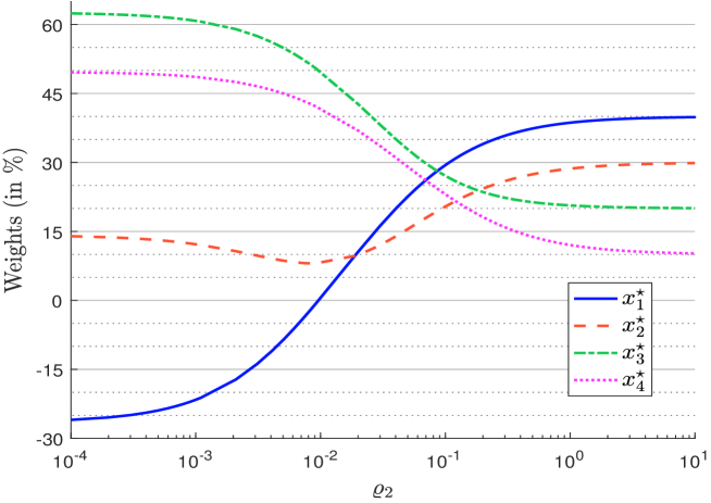
Figure 1: Ridge regularization with a target portfolio

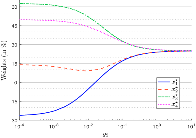
Figure 2: Ridge regularization without a target portfolio

We notice that the ridge regularization impacts entirely the covariance matrix. Indeed, the shrinkage volatilities are equal to $\sqrt{\sigma_{i}^{2}+\varrho_{2}}$ whereas the shrinkage correlation matrix is defined by:

$$\left[\mathcal{C}\left(\varrho_{2}\right)\right]_{i,j}=\rho_{i,j}\frac{\sigma_{i}\sigma_{j}}{\sqrt{\left(\sigma_{i}^{2}+\varrho_{2}\right)\left(\sigma_{j}^{2}+\varrho_{2}\right)}}$$

It follows that $\lim_{\varrho_{2}\rightarrow\infty}\mathcal{C}\left(\varrho_{2}\right)=I_{n}$. Since the volatilities tend to $\infty$, the ridge regularization can be viewed as a shrinkage covariance method between the input covariance matrix $\Sigma$ and the identity matrix:

$$\Sigma\left(\alpha\right)=\alpha\Sigma+\left(1-\alpha\right)I_{n}$$

Remark 5

A variant of the ridge regularization is to define $\Gamma_{2}$ as a diagonal matrix. For instance, if $\Gamma_{2}=\mathop{\rm diag}\Sigma$, the regularized correlation matrix satisfies:

$$\left[\mathcal{C}\left(\varrho_{2}\right)\right]_{i,j}=\frac{\rho_{i,j}}{1+\varrho_{2}}$$

In Figure 3, we have reported the impact of the parameter $\varrho_{2}$ on the correlation values.

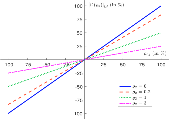
Figure 3: Impact of the parameter $\varrho$ on the correlation (diagonal ridge regularization)

3.4 Spectral filtering

Spectral filtering is a general approach based on the singular value decomposition (SVD) of the matrix $A_{1}$. Ridge regularization and denoising techniques can be seen as special cases of the SVD method.

3.4.1 General filters

We consider the SVD decomposition of the matrix $A_{1}$ by assuming that $\mathop{\rm rank}A_{1}=r$:

$$A_{1}=USV^{\top}$$

where the matrices $U\in\mathbb{R}^{n\times r}$, $V\in\mathbb{R}^{n\times r}$, $s=\left(s_{1},\ldots,s_{r}\right)\in\mathbb{R}^{r}$ and $S=\mathop{\rm diag}\left(s\right)$ satisfy $U^{\top}U=V^{\top}V=I_{r}$ and $s_{k}\geqslant s_{k+1}>0$. The Moore-Penrose pseudo-inverse of $A_{1}$ can be defined as:

$$A_{1}^{\dagger}=VS^{-1}U^{\top}$$

where $S^{-1}=\mathop{\rm diag}\left(s^{\dagger}\right)$. Let us denote $s_{\max}\left(A_{1}\right)=s_{1}$ the largest singular value of $A_{1}$.

As instability is raised by small eigenvalues, filtering can be applied to keep eigenvalues away from $0$. A filter $\mathcal{G}\left(s;\varrho\right)=\left(G\left(s_{1};\varrho\right),\ldots,G\left(s_{r};\varrho\right)\right)$ is a vector-valued function, where the $k^{\mathrm{th}}$ entry $G\left(s_{k};\varrho\right):\left]0,s_{\max}\left(A\right)\right]\rightarrow\mathbb{R}$ satisfies:

$$\lim_{\varrho\rightarrow 0}G\left(s_{k};\varrho\right)=\frac{1}{s_{k}}$$

for all $\varrho\geqslant 0$ and $s_{k}\in\left]0,s_{\max}\left(A\right)\right]$. The parameter $\varrho$ controls the magnitude of the regularization of $A_{1}^{\dagger}$:

$$A_{1}^{\dagger}\left(\varrho\right)=V\mathop{\rm diag}\left(\mathcal{G}\left(s;\varrho\right)\right)U^{\top}$$

As a consequence, we verify the property of convergence:

$$\lim_{\varrho\rightarrow 0}A_{1}^{\dagger}\left(\varrho\right)=A_{1}^{\dagger}$$

This method can be extended to regularize the matrix $A_{1}^{\top}A_{1}$. On one hand, if $A_{1}$ has full rank, we can approximate $Q=A_{1}^{\top}A_{1}$ by $A_{1}^{\top}\left(A_{1}^{\dagger}\left(\varrho\right)\right)^{-1}$. On the other hand, a direct computation leads to $Q=A_{1}^{\top}A_{1}=VS^{2}V^{\top}$. Therefore, we can regularize $Q=A_{1}^{\top}A_{1}$ by:

$$Q\left(\varrho\right)=V\mathop{\rm diag}\left(s^{2}\left(\varrho\right)\right)V^{\top}$$

where $s^{2}\left(\varrho\right)$ is a vector that may be equal to $\mathcal{G}\left(s;\varrho\right)^{\dagger}\,\odot\,\mathcal{G}\left(s;\varrho\right)^{\dagger}$, or $\mathcal{G}\left(s\odot s;\varrho\right)^{\dagger}$ or $\mathcal{G}\left(s;\varrho\right)^{\dagger}\,\odot\,s$. Once again, we have the convergence property:

$$\lim_{\varrho\rightarrow 0}Q\left(\varrho\right)=A_{1}^{\top}A_{1}$$

If we consider the problem:

$$x^{\star} = \arg\min\frac{1}{2}\left\|A_{1}x-b_{1}\right\|_{2}^{2}$$

s.t. $$A_{2}x=b_{2}$$

the normal equations are:

$$\left(\begin{array}[]{cc}A_{1}^{\top}A_{1}&A_{2}^{\top}\\ A_{2}&\mathbf{0}\end{array}\right)\left(\begin{array}[]{c}x\\ \lambda\end{array}\right)=\left(\begin{array}[]{c}A_{1}^{\top}b_{1}\\ b_{2}\end{array}\right)$$ (16)

Spectral filtering is then equivalent to replacing the linear system (16) by the following set of normal equations:

$$\left(\begin{array}[]{cc}V\mathop{\rm diag}\left(s^{2}\left(\varrho\right)\right)V^{\top}&A_{2}^{\top}\\ A_{2}&\mathbf{0}\end{array}\right)\left(\begin{array}[]{c}x\\ \lambda\end{array}\right)=\left(\begin{array}[]{c}U\mathop{\rm diag}\left(\mathcal{G}\left(s;\varrho\right)^{\dagger}\right)V^{\top}b_{1}\\ b_{2}\end{array}\right)$$ (17)

3.4.2 Application to Tikhonov regularization

To define the spectral regularization of the Tikhonov problem, the matrices $A_{1}$ and $\Gamma_{2}$ have to be able to be factored in a coherent way:

$$A_{1}=US_{1}V^{\top}$$

and:

$$\Gamma_{2}=WS_{2}V^{\top}$$

Direct computations gives:

$$A_{1}^{\top}A_{1}+\varrho_{2}\Gamma_{2}^{\top}\Gamma_{2}=V\left(S_{1}^{2}+\varrho_{2}S_{2}^{2}\right)V^{\top}$$

We deduce that the $k^{\mathrm{th}}$ entry of the spectral filter $\mathcal{G}\left(s_{1};\varrho_{2}\right)$ is defined by:

$$G\left(s_{1,k};\varrho_{2}\right)=\frac{s_{1,k}}{s_{1,k}^{2}+\varrho_{2}s_{2,k}^{2}}$$

Using the previous notations, we have:

$$\varrho_{2}\Gamma_{2}^{\top}\Gamma_{2} = A_{1}^{\top}A_{1}+\varrho_{2}\Gamma_{2}^{\top}\Gamma_{2}-A_{1}^{\top}A_{1}$$

$$= V\mathop{\rm diag}\left(s_{1}^{2}\left(\varrho_{2}\right)\right)V^{\top}-V\mathop{\rm diag}\left(s_{1}\odot s_{1}\right)V^{\top}$$

$$= V\mathop{\rm diag}\left(s_{1}^{2}\left(\varrho_{2}\right)-s_{1}^{2}\right)V^{\top}$$

where $s_{1}^{2}=s_{1}\odot s_{1}$. In this case, the optimal portfolio $x^{\star}$ is the $x$-coordinate of the solution to the linear system:

$$\left(\begin{array}[]{cc}V\mathop{\rm diag}\left(s_{1}^{2}\left(\varrho_{2}\right)\right)V^{\top}&A_{2}^{\top}\\ A_{2}&\mathbf{0}\end{array}\right)\left(\begin{array}[]{c}x\\ \lambda\end{array}\right)=\left(\begin{array}[]{c}A_{1}^{\top}b_{1}+V\mathop{\rm diag}\left(s_{1}^{2}\left(\varrho_{2}\right)-s_{1}^{2}\right)V^{\top}x_{0}\\ b_{2}\end{array}\right)$$ (18)

We notice that only the right singular vectors appear in Equation (18). Ridge regularization can be viewed as particular filters. More generally, when $A_{1}$ and $\Gamma_{2}$ have the same right singular vectors, Tikhonov regularization can be stated in terms of a filter.

In Figure 4, we report the spectral filter of the ridge regularization. The spectral filtering approach includes another popular method, which is the denoising method (Laloux et al., 1999):

$$G\left(s_{1,k};\varrho_{2}\right)=\mathbf{1}\left\{\left|s_{1,k}\right|\geqslant\varrho_{2}\right\}\cdot s_{1,k}^{\dagger}$$

We notice that deleting singular values is equivalent to applying a hard thresholding method while ridge regularization is a smoothing approach.

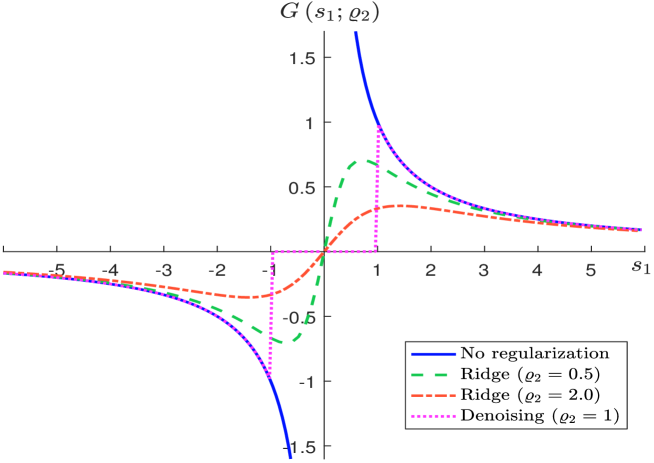
Figure 4: Spectral filtering (ridge regularization and denoising method)

3.4.3 Improvement of the stability condition

The condition number $\kappa\left(A\right)$ of the matrix $A$ summarizes the level of difficulty when performing the optimization in a stable way. More specifically, it measures how much an error on the vector $b$ changes the solution of the linear equation $Ax=b$. We have:

$$\kappa\left(A\right)=\left\|A^{\dagger}\right\|\cdot\left\|A\right\|$$

It follows that $\kappa\left(A^{\dagger}\right)=\kappa\left(A\right)$, and we have the property $\kappa\left(A\right)\geqslant 1$. When $\kappa\left(A\right)$ is low, the problem is numerically stable and easy to solve. The closer to one, the better the stability.

With the $L_{\infty}$ norm, we obtain:

$$\kappa\left(A\right)=\frac{\max_{k}\left|s_{k}\right|}{\min_{k}\left|s_{k}\right|}$$ (19)

where the $s_{k}$’s are the singular values of $A$. Using the filter $\mathcal{G}\left(s;\varrho\right)$, we obtain:

$$\kappa\left(A^{\dagger}\left(\varrho\right)\right)=\frac{\min_{k}\left|G\left(s_{k};\varrho\right)\right|}{\max_{k}\left|G\left(s_{k};\varrho\right)\right|}$$ (20)

For a fixed value of $\varrho>0$, all previous filters satisfy the two following properties:

1. $G\left(s_{k};\varrho\right)\sim s_{k}^{-1}$ for $s_{k}\rightarrow\infty$;

2. $G\left(s_{k};\varrho\right)$ is bounded from above on $\left[0,+\infty\right)$.

As a consequence, if we compare Equations (19) and (20), the denominator is essentially unchanged while the numerator is decreased. Therefore, spectral filtering decreases the condition number of $A$, because these techniques reduce the dispersion of singular values.

3.5 Mixed penalties

The Euclidian regularization is natural because the $L_{2}$ norm appears in Problem (3). Explicit formulas are obtained, and can be implemented at once. Other regularization techniques have been introduced to impose other constraints on the optimal solution $x^{\star}$. As the unit ball for the $L_{1}$ norm is not uniformly convex, sparse solutions may be obtained by penalizing with $L_{1}$ instead of $L_{2}$.

3.5.1 $L_{p}$ regularization

Instead of Tikhonov regularization, one may consider the $L_{p}$ regularization:

$$x^{\star} = \arg\min\frac{1}{2}\left\|A_{1}x-b_{1}\right\|_{2}^{2}+\frac{1}{p}\varrho_{p}\left\|\Gamma_{p}\left(x-x_{0}\right)\right\|_{p}^{p}$$

s.t. $$A_{2}x=b_{2}$$

where $x_{0}\in\mathbb{R}^{n}$ is a targeted portfolio and $p>0$.

For $p>1$, the function $\Gamma_{p}\left(x\right)=\left\|\Gamma_{p}\left(x-x_{0}\right)\right\|_{p}^{p}$ is strictly convex and its gradient is Lipschitz continuous. Indeed, the gradient is equal $p\Gamma_{p}^{\top}\mathop{\rm sign}\left(\Gamma_{p}\left(x-x_{0}\right)\right)\odot\left|\Gamma_{p}\left(x-x_{0}\right)\right|^{p-1}$, where the functions $\mathop{\rm sign}\left(x\right)$ and $\left|x\right|$ are taken component wise. For $p=1$, the function $\Gamma_{1}\left(x\right)$ is convex, lower semi-continuous but may not be differentiable at $x=x_{0}$. An explicit expression for its subgradient can be formulated in terms of proximal operators. For $p\in\left]0,1\right[$, the function $\Gamma_{p}\left(x\right)$ is not convex, and Problem (3.5.1) is not convex.

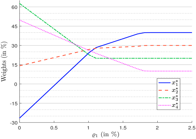
Figure 5: Lasso regularization with a target portfolio

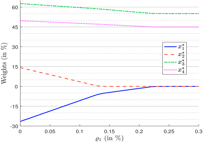
Figure 6: Lasso regularization without a target portfolio

The penalties $L_{p}$ for $p\geqslant 1$ are used for regularization, while the penalties $L_{p}$ for $p\leqslant 1$ are used for sparsity. The case $p=1$ is the most interesting since it corresponds to the lasso regression (Tibshirani, 1996). In this case, a large value of $\varrho_{1}$ associated with the constraint $\mathbf{1}^{\top}x=1$ forces the optimal portfolio to have long-only positions (Brodie et al., 2009).

We consider the example given on page 3.3.3. We use a $L_{1}$ (or lasso) penalty with $\Gamma_{1}=I_{n}$. Figure 5 show the optimal weights with respect to the penalization factor $\varrho_{1}$. Like in the ridge approach, the optimized portfolio converges to the optimal portfolio when the parameter $\varrho$ increases. When there is no target portfolio, we observe a divergence of the limit portfolio between ridge and lasso approaches. While the ridge portfolio converges to the equally-weighted portfolio, the lasso portfolio converges to the long-only mean-variance optimized portfolio (Figure 6). If we compare Figures 1 and 5, we notice that the magnitude of the regularization factor is not the same. We also observe that the paths are different. The path is smoothed and continuous for the ridge approach, while it is more a piecewise linear function for the lasso approach. We verify that the $L_{1}$ penalty produces a sparse optimized portfolio. This is obvious for the case where there is no target portfolio since weights may be equal to zero. When there is a target portfolio, the sparsity concerns the bets between the optimized portfolio $x^{\star}$ and the target portfolio $x_{0}$. In this case, relative (and not absolute) weights are equal to zero. Another difference between the two approaches is that the lasso method produces a monotonic path (decreasing or increasing) contrary to the ridge method.

3.5.2 $L_{1}-L_{2}$ regularization

We can also consider a mixed penalty:

$$x^{\star} = \arg\min\frac{1}{2}\left\|A_{1}x-b_{1}\right\|_{2}^{2}+\varrho_{p}\left\|\Gamma_{p}\left(x-x_{0}\right)\right\|_{p}^{p}+\frac{1}{2}\varrho_{2}\left\|\Gamma_{2}\left(x-x_{0}\right)\right\|_{2}^{2}$$

s.t. $$A_{2}x=b_{2}$$

where $p\neq 2$. In the case $p=1$, we obtain:

$$x^{\star} = \arg\min\frac{1}{2}\left\|A_{1}x-b_{1}\right\|_{2}^{2}+\varrho_{1}\left\|\Gamma_{1}\left(x-x_{0}\right)\right\|_{1}+\frac{1}{2}\varrho_{2}\left\|\Gamma_{2}\left(x-x_{0}\right)\right\|_{2}^{2}$$

s.t. $$A_{2}x=b_{2}$$

This regularization is called elastic net (Hastie et al., 2009). This is the most common mixed penalty used in portfolio optimization (Roncalli, 2013).

We consider again the example given on page 3.3.3. We use a lasso-ridge penalty with $\Gamma_{1}=\Gamma_{2}=I_{n}$. Results are reported in Figures 7 and 8. We notice a large difference concerning the convergence. Indeed, we recall that the lasso and ridge approaches converge to the same portfolio when we impose a target portfolio, but to two different portfolios when there is no target portfolio. When mixing the two norms, the limit portfolio is generally the ridge portfolio, because of the magnitude of $\varrho_{1}$ and $\varrho_{2}$ in portfolio management (see Appendix A.5 on page A.5). This result is true because we have imposed $\Gamma_{1}=\Gamma_{2}=I_{n}$.

Figure 7: Mixed regularization with a target portfolio

Figure 8: Mixed regularization without a target portfolio

3.5.3 Solving the mixed penalty problem

Problems (3.5.2) and (3.5.2) are more complex to solve than a traditional quadratic programming problem. In the case of the $L_{1}-L_{2}$ regularization problem and if we assume that $\Gamma_{1}$ is a matrix with non-negative entries, we can use a modified QP solver. The underlying idea is to write $\Gamma_{1}\left(x\right)$ in the following way:

$$\Gamma_{1}\left(x\right)=\mathbf{1}^{\top}\Gamma_{1}\delta^{-}+\mathbf{1}^{\top}\Gamma_{1}\delta^{+}$$

where $\delta^{-}=\max\left(\mathbf{0},x_{0}-x\right)$ and $\delta^{+}=\max\left(\mathbf{0},x-x_{0}\right)$. Therefore we obtain a standard QP problem by augmenting the vector of unknown variables. Thus, the optimization is performed with respect to $y=\left(x,\delta^{-},\delta^{+}\right)$ and no longer with respect to $x$. In the other cases, when we consider an $L_{p}$ penalty with $p\neq 2$ or when $\Gamma_{1}$ is a matrix with some negative entries, the general approach is to use the ADMM algorithm, which is described in Appendix A.7 on page A.7. For instance, Problem (3.5.2) can be written as:

$$\left\{x^{\star},z^{\star}\right\} = \arg\min f\left(x\right)+g\left(z\right)$$

s.t. $$x-z=\mathbf{0}$$

where:

$$f\left(x\right)=\frac{1}{2}\left\|A_{1}x-b_{1}\right\|_{2}^{2}+\frac{1}{2}\varrho_{2}\left\|\Gamma_{2}\left(x-x_{0}\right)\right\|_{2}^{2}+\mathds{1}_{\Omega}\left(x\right)$$

and:

$$g\left(z\right) = \varrho_{1}\Gamma_{1}\left(x\right)$$

$$= \varrho_{1}\left\|\Gamma_{1}\left(x-x_{0}\right)\right\|_{1}$$

where $\Omega=\left\{x\in\mathbb{R}^{n}:A_{2}x=b_{2}\right\}$. The interest of this choice is that the $x$-step includes the constraint and can be explicitly computed, while the $z$-step requires to compute the proximal operator of the function $\Gamma_{1}\left(x\right)$:

$$z^{\left(k+1\right)}=\arg\min\left\{g\left(z\right)+\frac{\varphi}{2}\left\|x^{\left(k+1\right)}-z+u^{\left(k\right)}\right\|_{2}^{2}\right\}$$

The update of the scaled dual variable is:

$$u^{\left(k+1\right)}=u^{\left(k\right)}+\left(x^{\left(k+1\right)}-z^{\left(k+1\right)}\right)$$

The previous results can be extended when $p\neq 1$ and $\Omega$ is a set of more complex constraints.

Appendices A.7 and A.8 on pages A.7–A.8.3 contain all the information for solving the following optimization problem:

$$x^{\star} = \arg\min\frac{1}{2}\left\|A_{1}x-b_{1}\right\|_{2}^{2}+\varrho_{p}\left\|\Gamma_{p}\left(x-x_{0}\right)\right\|_{p}^{p}+\frac{1}{2}\varrho_{2}\left\|\Gamma_{2}\left(x-x_{0}\right)\right\|_{2}^{2}$$

s.t. $$x\in\Omega$$

where $\Omega$ may be equality, inequality, bound and $L_{q}$ norm constraints.

3.6 Optimal choice of the regularization factor

To choose the optimal regularization parameter, we first have to define an optimization criterion. For instance, the optimal value of $\varrho_{1}$ or $\varrho_{2}$ is generally obtained by cross-validation techniques. Exhaustive methods such as leave-$p$-out cross-validation (LpOCV) or leave-one-out cross-validation (LOOCV) are computationally intensive. This is why it may be better to use non-exhaustive methods such as $k$-fold cross-validation or out-of-sample testing. However, in the case of the Tikhonov regularization, an explicit formula is known. Indeed, the generalized cross-validation procedure for choosing $\varrho_{2}$ does not depend on the dual variable or the constraints. In the case of the $L_{1}$ penalty, no explicit formula is known and the brute force algorithm must be used for finding the optimal value of $\varrho_{1}$.

3.6.1 Cross-validation and the PRESS statistic

Let us consider the data matrix $X=\left(x_{1}^{\top},\ldots,x_{T}^{\top}\right)\in\mathbb{R}^{T\times K}$ where $x_{t}\in\mathbb{R}^{K}$, and a response vector $Y=\left(y_{1},\ldots,y_{T}\right)\in\mathbb{R}^{T}$ where $y_{t}\in\mathbb{R}$. Since the Tikhonov regularization problem is defined as follows:

$$\hat{\beta}=\arg\min\frac{1}{2}\left\|Y-X\beta\right\|_{2}^{2}+\frac{1}{2}\varrho_{2}\left\|\Gamma_{2}\beta\right\|_{2}^{2}$$

we have:

$$\hat{\beta}=S\left(\varrho_{2}\right)X^{\top}Y$$

where:

$$S\left(\varrho_{2}\right)=\left(X^{\top}X+\varrho_{2}\Gamma_{2}\Gamma_{2}^{\top}\right)^{-1}$$

It follows that $\hat{\beta}$ is a function of $\varrho_{2}$. Therefore, the underlying idea is to find the optimal value $\hat{\varrho}_{2}$.

In order to accurately estimate the hyperparameters of the model and to avoid overfitting problems, the cross-validation (CV) method comprises several steps:

1. the sample of data is partitioned into two sets, the training set and the test (or validation) set;

2. the model is fitted on the training set;

3. the model is tested on the validation set.

In order to reduce variability, steps 2 and 3 are performed using different partitions of the data sample (step 1). The validation results are combined, according to a measure of fit, to give an estimate of the model predictive performance. The hyperparameters are then chosen in order to maximize this goodness-of-fit measure. Two types of CV may be performed: exhaustive and non-exhaustive cross-validation. For the first type, the model is estimated and tested on all possible ways to divide the original sample into training/test sets. This type of CV consists of the leave-$p$-out cross validation (LpOCV). In this approach, $p$ observations are used in the test set and the remaining observations are used in the training set. This requires training and validating the model $\binom{T}{p}$ times, which can be extremely expensive if $T$ is large, even for $p=1$. Nevertheless, an explicit expression for the sum of squares of the errors is known in the case of Tikhonov regression. This formula may lead to $O\left(T\right)$ operations. For this reason, non-exhaustive cross-validation may be preferred in practice, such as $k$-fold CV, holdout method, repeated random sub-sampling, jackknife, etc. Performing $k$-fold CV is the most popular tool for model selection (Stone, 1974; Wahba, 1977; Stone, 1978).

In $k$-fold CV, the sample of data is randomly shuffled and split into $k$ (almost) equally sized groups, the model is fitted using all but the $j^{\mathrm{th}}$ group of data, and the $j^{\mathrm{th}}$ group of data is used for the test set. We repeat the procedure $k$ times, in such a way that each group is tested exactly once. The $k$-fold cross validated error is generally computed as:

$$\mathcal{E}_{\mathrm{cv}}=\frac{1}{T}\sum_{j=1}^{k}\sum_{t\in\mathcal{G}_{k}}\left(y_{t}-x_{t}^{\top}\beta\left(k\right)\right)^{2}$$

where $t\in\mathcal{G}_{k}$ denotes the observations of the $k^{\mathrm{th}}$ group and $\beta\left(k\right)$ the estimation of $\beta$ obtained by leaving out the $k^{\mathrm{th}}$ group. Even in simple cases, it cannot be guaranteed that the function $\mathcal{E}_{\mathrm{cv}}$ has a unique minimum. The simple grid search approach is probably the best approach. The exhaustive Leave-one-out cross validation (LOOCV) is a particular case when $k$ is equal to the size of the dataset. The LOOCV is asymptotically equivalent to Akaike Information Criterion (AIC), which is commonly used in statistics (Stone, 1977). Interestingly, For Tikhonov regression, the cross validated error $\mathcal{E}_{\mathrm{cv}}$ has an explicit expression known as the Predicted Sum of Squares (or PRESS) statistic (Allen, 1971 & 1974).

We note $Y_{-t}$ and $X_{-t}$ the $\left(T-1\right)$ vector and $\left(T-1\right)\times K$ matrix by leaving out the $t^{th}$ observation to the vector $Y$ and the matrix $X$. We have:

$$\hat{\beta}_{-t}=\left(X_{-t}^{\top}X_{t}+\varrho_{2}\Gamma_{2}\Gamma_{2}^{\top}\right)^{-1}X_{-t}^{\top}Y_{-t}$$

The explicit expression for the LOOCV procedure is:

$$\mathcal{P}\mathrm{ress}\left(\varrho_{2}\right) = \sum_{t=1}^{T}\left(y_{t}-x_{t}^{\top}\hat{\beta}_{-t}\right)^{2}$$

$$= \sum_{t=1}^{T}\left(1-x_{t}^{\top}S\left(\varrho_{2}\right)x_{t}\right)^{-2}\left(y_{t}-x_{t}^{\top}\hat{\beta}\right)^{2}$$

$$= \sum_{t=1}^{T}\left(\frac{\left[\mathbf{L}\left(\varrho_{2}\right)Y\right]_{t}}{\left[\mathbf{L}\left(\varrho_{2}\right)\right]_{t,t}}\right)^{2}$$

where $\mathbf{L}\left(\varrho_{2}\right)$ is the projection matrix defined as:

$$\mathbf{L}\left(\varrho_{2}\right) = I_{T}-XS\left(\varrho_{2}\right)X^{\top}$$

$$= I_{T}-X\left(X^{\top}X+\varrho_{2}\Gamma_{2}\Gamma_{2}^{\top}\right)^{-1}X^{\top}$$

If $S\left(\varrho_{2}\right)$ is a band matrix, which is the case for spline models, the coefficients $\left[\mathbf{L}\left(\varrho_{2}\right)\right]_{t,t}$ and $\left[\mathbf{L}\left(\varrho_{2}\right)Y\right]_{t}$ can be computed in $O\left(T\right)$ operations thanks to the Hutchinson-De Hoog algorithm (Hutchinson and De Hoog, 1985).

3.6.2 GCV for centered data as the selection criterion

The generalized cross-validation (GCV) method is a rotation-invariant version of LOOCV (Craven and Wahba, 1978). Even if it is not its main purpose, this approach replaces the factor $\left[\mathbf{L}\left(\varrho_{2}\right)\right]_{t,t}$ by the average value $T^{-1}\mathop{\rm trace}\mathbf{L}\left(\varrho_{2}\right)$:

$$GCV\left(\varrho_{2}\right)=\frac{T^{2}}{\mathop{\rm trace}^{2}\mathbf{L}\left(\varrho_{2}\right)}\sum_{t=1}^{T}\left(y_{t}-x_{t}^{\top}\hat{\beta}\right)^{2}$$ (24)

We deduce that the GCV criterion depends on $\mathbf{L}\left(\varrho_{2}\right)$ and the residual sum of squares $\sum_{t=1}^{T}\left(y_{t}-x_{t}^{\top}\hat{\beta}\right)^{2}$. We recall that $\mathbf{H}\left(\varrho_{2}\right)=I_{T}-\mathbf{L}\left(\varrho_{2}\right)$ is the hat matrix. The value $\left[\mathbf{H}\left(\varrho_{2}\right)\right]_{t,t}$ is called the leverage value (Craven and Wahba, 1978) and determines the amount by which the predicted value $\hat{y}_{t}=x_{t}^{\top}\hat{\beta}$ is influenced by $y_{t}$. We also know that $\mathop{\rm trace}\mathbf{L}\left(\varrho_{2}\right)=T-K$. From the Woodbury formula, we have:

$$\mathbf{L}\left(\varrho_{2}\right) = I_{T}-X\left(X^{\top}X+\varrho_{2}\Gamma_{2}\Gamma_{2}^{\top}\right)^{-1}X^{\top}$$

$$= \left(I_{T}+X\left(\varrho_{2}\Gamma_{2}\Gamma_{2}^{\top}\right)^{-1}X^{\top}\right)^{-1}$$

Let $\lambda_{t}$ be the eigenvalues of the symmetric real matrix $X\left(\Gamma_{2}\Gamma_{2}^{\top}\right)^{-1}X^{\top}$. We have:

$$\mathop{\rm trace}\mathbf{L}\left(\varrho_{2}\right)=\sum_{t=1}^{T}\left(1+\frac{\lambda_{t}}{\varrho_{2}}\right)^{-1}$$

This formula allows the value of $\mathop{\rm trace}^{-2}\mathbf{L}\left(\varrho_{2}\right)$ to be computed for every value of $\varrho_{2}$. Like the PRESS statistic, the optimal value of $\varrho_{2}$ is obtained by minimizing the GCV function given by Equation (24).

4 Application to robo-advisory

The previous techniques are of particular interest for portfolio optimization when building a strategic asset allocation (SAA), a trend-following strategy or more generally a mean-variance diversified portfolio. Depending on the approach, they can diversify or concentrate the portfolio. By mixing the different approaches, we can also obtain a diversified allocation on some selected stocks. In this case, portfolio regularization and portfolio sparsity are combined. The previous techniques can also be used when implementing tactical asset allocation (TAA). In this case, regularization and sparsity are imposed in a relative way with respect to a benchmark or a current investment portfolio. In this section, we show why these techniques are necessary when building a robo-advisor based on an automated allocation engine.

4.1 Robo-advisory and the secret sauce of portfolio optimization

The idea that portfolio optimization is a simple mathematical problem is mistaken. It is a process that requires manual interventions and may take considerable time before a solution is found. And this human intervention has little in common with numerical algorithms. Indeed, Quants know that the secret sauce of portfolio optimization lies in the alchemy of defining the right constraints in order to obtain an acceptable solution that makes sense. Let us consider the traditional strategic asset allocation exercise that is performed by institutional investors almost every year. We assume that the SAA team has already produced the two inputs: the vector $\mu$ of expected returns and the covariance $\Sigma$ of asset returns. We could think that the hard work has therefore been done, and that computing the SAA portfolio will take a matter of seconds since we just have to run a Markowitz optimization. In reality, solving one Markowitz optimization generally produces a bad solution and is not sufficient. This is why Quants will use an iterative process based on this optimization program:

$$x_{\left(k\right)}^{\star} = \arg\min\frac{1}{2}x^{\top}\Sigma x-\gamma x^{\top}\mu$$ (25)

s.t. $$\left\{\begin{array}[]{l}\mathbf{1}^{\top}x=1\\ \mathbf{0}\leqslant x\leqslant\mathbf{1}\\ x\in\Omega_{\left(k\right)}\end{array}\right.$$ (29)

where $\Omega_{\left(0\right)}=\mathbb{R}^{n}$ and $k$ is the step. They will begin by solving the traditional Markowitz problem with long-only constraints and will find an initial solution $x_{\left(0\right)}^{\star}$. Then, they will analyze this solution and define a new set of constraints $\Omega_{\left(1\right)}$ that might produce a more acceptable solution. The concept of “acceptable solution” remains unclear, but it means one that can be accepted by the chief investment officer. Once $\Omega_{\left(1\right)}$ is defined, Quants will run the optimization problem (25) and obtain a new solution $x_{\left(1\right)}^{\star}$. Next, they will analyze this new solution and define a new set of constraints $\Omega_{\left(2\right)}$ that might produce an even more acceptable solution. They will iterate this process a number of times. Therefore, this iterative process can be represented by the sequence $\boldsymbol{P}$ defined as follows:

$$\boldsymbol{P}=\left\{x_{\left(0\right)}^{\star},\Omega_{\left(1\right)},x_{\left(1\right)}^{\star},\Omega_{\left(2\right)},x_{\left(2\right)}^{\star},\Omega_{\left(3\right)},x_{\left(3\right)}^{\star},\ldots\right\}$$

Using this tool, we can evaluate Quants and draw some conclusions:

• A good Quant is a person that is able to “close” this sequence in a limited number of steps.

• A bad Quant is a person that produces an infinite sequence and is not able to end the process.

• Quant $Q_{1}$ is more efficient than Quant $Q_{2}$ if:

  $$\mathop{\rm card}\boldsymbol{P}\left(Q_{1}\right)<\mathop{\rm card}\boldsymbol{P}\left(Q_{2}\right)$$

Let us illustrate the previous process with an example. We consider a universe of nine asset classes: (1) US 10Y Bonds, (2) Euro 10Y Bonds, (3) Investment Grade Bonds, (4) High Yield Bonds, (5) US Equities, (6) Euro Equities, (7) Japan Equities, (8) EM Equities and (9) Commodities. In Tables 12 and 13, we indicate the statistics used to compute the optimal allocation. The objective is to find the optimal allocation for an ex-ante volatility of around $7\%$.

Table 12: Expected returns and risks (in %)

	(1)	(2)	(3)	(4)	(5)	(6)	(7)	(8)	(9)
$\mu_{i}$	${\hskip 5.0pt}4.2$	${\hskip 5.0pt}3.8$	${\hskip 5.0pt}5.3$	$10.4$	${\hskip 5.0pt}9.2$	${\hskip 5.0pt}8.6$	${\hskip 5.0pt}5.3$	$11.0$	${\hskip 5.0pt}8.8$
$\sigma_{i}$	${\hskip 5.0pt}5.0$	${\hskip 5.0pt}5.0$	${\hskip 5.0pt}7.0$	$10.0$	$15.0$	$15.0$	$15.0$	$18.0$	$30.0$

Table 13: Correlation matrix of asset returns (in %)

	(1)	(2)	(3)	(4)	(5)	(6)	(7)	(8)	(9)
(1)	${\hskip 3.0pt}100$
(2)	${\hskip 8.0pt}80$	${\hskip 3.0pt}100$
(3)	${\hskip 8.0pt}60$	${\hskip 8.0pt}40$	$100$
(4)	$-20$	$-20$	${\hskip 5.0pt}50$	$100$
(5)	$-10$	$-20$	${\hskip 5.0pt}30$	${\hskip 5.0pt}60$	$100$
(6)	$-20$	$-10$	${\hskip 5.0pt}20$	${\hskip 5.0pt}60$	${\hskip 5.0pt}90$	$100$
(7)	$-20$	$-20$	${\hskip 5.0pt}20$	${\hskip 5.0pt}50$	${\hskip 5.0pt}70$	${\hskip 5.0pt}60$	$100$
(8)	$-20$	$-20$	${\hskip 5.0pt}30$	${\hskip 5.0pt}60$	${\hskip 5.0pt}70$	${\hskip 5.0pt}70$	${\hskip 5.0pt}70$	$100$
(9)	${\hskip 13.0pt}0$	${\hskip 13.0pt}0$	${\hskip 5.0pt}10$	${\hskip 5.0pt}20$	${\hskip 5.0pt}20$	${\hskip 5.0pt}20$	${\hskip 5.0pt}30$	${\hskip 5.0pt}30$	$100$

Using these figures, we obtain an initial allocation $x^{\star}_{\left(0\right)}$ that is reported in Table 14. The optimal portfolio is invested in only four asset classes. The allocation in US 10Y Bonds is $28\%$, while the allocation in High Yield Bonds is $70\%$. It is obvious that this portfolio cannot be a SAA policy. This is why the Quant will add some constraints in order to obtain a better solution. We can impose that the weight of one asset class cannot exceed $25\%$. Using this new set of constraints $\Omega_{\left(1\right)}$, we obtain Portfolio $x^{\star}_{\left(1\right)}$ that is less concentrated than Portfolio $x^{\star}_{\left(0\right)}$. The allocation in US 10Y Bonds and High Yield Bonds reaches the cap of $25\%$. The portfolio is now invested in Euro 10Y Bonds ($15.90\%$), US Equities ($10.70\%$) and EM Equities ($21.27\%$). The drawback of this solution could be the allocation in equities, which is too small. This is why the Quant will add another constraint in order to obtain an equity allocation that is larger than $40\%$. At the third iteration, we then obtain Portfolio $x^{\star}_{\left(3\right)}$. If we assume that the SAA exercise is complete for a European institutional investor, this solution is not acceptable because it contains many US assets and too few European assets. This is why the Quant will add two new constraints. He can require that the allocation in Euro 10Y Bonds is larger than the allocation in US 10Y Bonds, and that the allocation in Euro Equities is larger than the allocation in US Equities. By using this new set of constraints $\Omega_{\left(4\right)}$, we obtain the following solution: the weight of US 10Y Bonds is $12.13\%$, the weight of Euro 10Y Bonds is $22.13\%$, the weight of IG Bonds is $15.00\%$, etc. Again, this solution may not be acceptable, because there is no allocation in Japanese equities. Therefore, the Quant may impose that there is at least $5\%$ invested in this asset class. After few additional iterations, the solution is given by the last column in Table 14.

Table 14: The iterative trial-and-error solutions

Step $k$		#0	#1	#2	#3	#4	$\cdots$	#K
US 10Y Bonds	(1)	$28.39$	$25.00$	$24.99$	$25.00$	$12.13$		$10.00$
Euro 10Y Bonds	(2)	${\hskip 5.0pt}0.00$	$15.90$	$18.60$	$16.50$	$22.13$		$30.00$
IG Bonds	(3)	${\hskip 5.0pt}0.00$	${\hskip 5.0pt}0.00$	${\hskip 5.0pt}0.00$	${\hskip 5.0pt}4.86$	$15.00$		$10.00$
HY Bonds	(4)	$69.64$	$25.00$	$16.41$	$10.00$	$10.00$		${\hskip 5.0pt}5.00$
US Equities	(5)	${\hskip 5.0pt}0.00$	$10.70$	$20.86$	$25.00$	$10.00$		$10.00$
Euro Equities	(6)	${\hskip 5.0pt}0.00$	${\hskip 5.0pt}0.00$	${\hskip 5.0pt}3.16$	${\hskip 5.0pt}5.00$	$20.00$		$20.00$
Japan Equities	(7)	${\hskip 5.0pt}0.00$	${\hskip 5.0pt}0.00$	${\hskip 5.0pt}0.00$	${\hskip 5.0pt}0.00$	${\hskip 5.0pt}0.00$		${\hskip 5.0pt}5.00$
EM Equities	(8)	${\hskip 5.0pt}1.17$	$21.27$	$15.98$	$10.00$	$10.00$		${\hskip 5.0pt}8.00$
Commodities	(9)	${\hskip 5.0pt}0.79$	${\hskip 5.0pt}2.13$	${\hskip 5.0pt}0.00$	${\hskip 5.0pt}3.64$	${\hskip 5.0pt}0.73$		${\hskip 5.0pt}2.00$
$\mu\left(x\right)$		${\hskip 5.0pt}8.63$	${\hskip 5.0pt}7.77$	${\hskip 5.0pt}7.41$	${\hskip 5.0pt}7.12$	${\hskip 5.0pt}6.99$		${\hskip 5.0pt}6.57$
$\sigma\left(x\right)$		${\hskip 5.0pt}7.00$	${\hskip 5.0pt}7.00$	${\hskip 5.0pt}7.00$	${\hskip 5.0pt}7.00$	${\hskip 5.0pt}7.00$		${\hskip 5.0pt}6.84$
$\mathop{\rm SR}\left(x\mid r\right)$		$80.49$	$68.08$	$63.03$	$58.93$	$57.00$		$52.17$

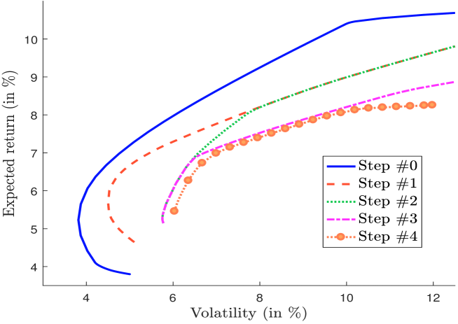
Figure 9: How does the secret sauce of portfolio optimization work?

We notice that the previous iterative process $\boldsymbol{P}$ satisfies:

$$\Omega_{\left(k+1\right)}\subset\Omega_{\left(k\right)}\subset\cdots\subset\Omega_{\left(2\right)}\subset\Omega_{\left(1\right)}$$

The underlying idea is to define an increasingly constrained investment universe. For instance, we verify that the efficient frontiers are ordered and that they are more and more constrained (see Figure 9).

Remark 6

Quants may use variants of Problem (25). When they are also in charge of producing $\mu$ and $\Sigma$, they may also consider the iterative process with the following optimization problem:

$$x_{\left(k\right)}^{\star}=\arg\min\frac{1}{2}x^{\top}\Sigma_{\left(k\right)}x-\gamma x^{\top}\mu_{\left(k\right)}$$

In this case, the sequence $\boldsymbol{P}$ is defined as follows:

$$\boldsymbol{P}=\left\{x_{\left(0\right)}^{\star},\Omega_{\left(1\right)},\Sigma_{\left(1\right)},\mu_{\left(1\right)},x_{\left(1\right)}^{\star},\Omega_{\left(2\right)},\Sigma_{\left(2\right)},\mu_{\left(2\right)},x_{\left(2\right)}^{\star},\ldots\right\}$$

It is obvious that the iterative process for defining the optimal portfolio conflicts with an automated and algorithm-driven robo-advisor. First, this is not the intent of a robo-advisor, unless we reduce the concept of robo-advisory to a digital application or a data-visualization tool, meaning that allocation decisions are made outside the robo-advisor. Second, a robo-advisor should be able to manage many portfolios on an industrial scale. If we consider the traditional lifestyle approach based on three portfolios (defensive, balanced and dynamic), which are rebalanced at the end of each month, it is obvious that the robo-advisor can be manually loaded every month. Again, this approach does not correspond to the robo-advisory concept. Indeed, robo-advisors claim that they better meet the expectations of investors by taking into account their constraints and by being more granular. This is particularly true with the emergence of goal-based investing in wealth management:

“While mass production has happened a long time ago in investment management through the introduction of mutual funds and more recently exchange traded funds, a new industrial revolution is currently under way, which involves mass customization, a production and distribution technique that will allow individual investors to gain access to scalable and cost-efficient forms of goal-based investing solutions” (Martellini, 2016, page 5).

Lastly, the iterative process does not help improve the portfolio management in a scientific manner. Indeed, it is a blind-eye approach, because it is difficult to explain the performance of the portfolio. We don’t know if it comes from the expected returns step (or the active bets) or the portfolio optimization step. In robo-advisory, these two steps must be easily identified and distinguished. Indeed, the portfolio optimization engine is part of the robo-advisor while expected returns may be designed outside the robo-advisor. This is generally the case because they can be imposed by the final investor himself, they can change from one third-party distributor to another, some investors will want to introduce trend-following patterns, etc. Contrary to the optimization method, the engine of expected returns is therefore not necessarily decided by the fintech that produces the robo-advisor. This is why the two steps must be perfectly differentiated.

4.2 Formulation of the optimization problem

We note $\tilde{x}$ the reference portfolio and $x_{t}$ the current portfolio. The optimized portfolio for the next period is the solution of this comprehensive optimization program:

$$x_{t+1}^{\star} = \arg\min f\left(x\right)+\tilde{\varrho}_{1}\left\|\tilde{\Gamma}_{1}\left(x-\tilde{x}\right)\right\|_{1}+\frac{1}{2}\tilde{\varrho}_{2}\left\|\tilde{\Gamma}_{2}\left(x-\tilde{x}\right)\right\|_{2}^{2}+$$

$$+\varrho_{1}\left\|\Gamma_{1}\left(x-x_{t}\right)\right\|_{1}+\frac{1}{2}\varrho_{2}\left\|\Gamma_{2}\left(x-x_{t}\right)\right\|_{2}^{2}$$

s.t. $$\left\{\begin{array}[]{l}\mathbf{1}^{\top}x=1\\ \mathbf{0}\leqslant x\leqslant\mathbf{1}\\ x\in\Omega\end{array}\right.$$ (34)

where $\Omega$ is a set of predetermined constraints. This problem considers both $L_{1}$ and $L_{2}$ penalty functions with respect to the reference portfolio and the current portfolio. Concerning $f\left(x\right)$, we can use the Markowitz function:

$$f\left(x\right)=\frac{1}{2}x^{\top}\Sigma x-\gamma x^{\top}\mu$$

However, it is certainly better to consider the tracking-error function with respect to the reference portfolio:

$$f\left(x\right) = \frac{1}{2}\left(x-\tilde{x}\right)^{\top}\Sigma\left(x-\tilde{x}\right)-\gamma\left(x-\tilde{x}\right)^{\top}\mu$$

$$= \frac{1}{2}x^{\top}\Sigma x-\gamma x^{\top}\left(\mu+\frac{1}{\gamma}\Sigma\tilde{x}\right)+C$$

where $C$ is a constant that does not depend on the variable $x$.

The aims of Problem (4.2) are multiple:

1. The first objective is naturally to optimize the traditional risk/return trade-off.

2. The second objective is to control the active bets between the reference portfolio $\tilde{x}$ and the new optimized portfolio $x_{t+1}^{\star}$ at various levels:

   1. The first layer is to target a tracking error by using the TE objective function in place of the MVO objective function;

   2. The second layer is the $L_{2}$ penalty $\tilde{\varrho}_{2}\left\|\tilde{\Gamma}_{2}\left(x-\tilde{x}\right)\right\|_{2}^{2}$ that helps to smooth the tactical allocation with respect to the strategic allocation. This layer implies shrinking the covariance matrix $\Sigma$;

   3. The third layer is the $L_{1}$ penalty $\tilde{\varrho}_{1}\left\|\tilde{\Gamma}_{1}\left(x-\tilde{x}\right)\right\|_{1}$ that helps to sparsify the relative bets with respect to Portfolio $\tilde{x}$;

3. The third objective is to control the turnover ($L_{1}$ penalty) and the quadratic costs ($L_{2}$ penalty) with respect to the current portfolio $x_{t}$.

With all these safeguards, we are equipped to perform stable and robust dynamic allocation for robo-advisors. However, three issues remain unsolved: the specification of expected returns, the choice of the tracking error level and the calibration of the regularization parameters. The idea of the next section is not to give a solution or to publish our know-how on these topics (Malongo et al., 2016). However, we will indicate the shortcomings to be avoided.

4.3 Practical considerations

4.3.1 Incorporating active management views

In some cases, robo-advisors are closed systems, but most of the time, they are open systems. Often, the fintech that developed the robo-advisor technology enters into bilateral agreements with third-party distributors (asset managers, private banks, wealth managers, insurance companies, retail distributors, etc.). In this case, the robo-advisor platform is adapted to take into account the distributor’s specific requirements, constraints and objectives. For instance, the robo-advisor platform may be plugged with the distributor’s risk/return profiling system. The number of funds and the investment universe changes from one distributor to another one. One of the big specific features is the engine that produces expected returns. It is rare that the distributor uses the default engine provided by the fintech. For instance, some investors will want to incorporate momentum patterns, others prefer to use expected returns produced by their economic experts, etc.

In practice, it is extremely difficult to express bets in terms of absolute returns. Portfolio managers prefer to use a rating scale $\mathcal{S}$ with different grades. The typical rating scale contains $7$ grades:

Grade Definition

$$---$$ Strong bearish

Bearish

Weak bearish

Neutral

Weak bullish

Bullish

Strong bullish

The challenge is then to transform these grades into expected returns. The most frequent empirical approach is based on the Black-Litterman model, which is described in Appendix B on page B.

Given a strategic portfolio $\tilde{x}$, we compute the implied expected returns $\tilde{\mu}_{i}$ of Asset $i$ thanks to the CAPM equation:

$$\tilde{\mu}_{i}=r+\mathop{\rm SR}\left(\tilde{x}\mid r\right)\frac{\left(\Sigma\tilde{x}\right)_{i}}{\sqrt{\tilde{x}^{\top}\Sigma\tilde{x}}}$$ (35)

We assume that the signal $s_{i}$ on Asset $i$ is homogeneous to a Sharpe ratio. In particular, we have:

$$\Delta\mathop{\rm SR}{}_{i}=\delta\frac{s_{i}}{n_{s}}$$

where $n_{s}$ is the range index of the rating scale and $\delta$ is a scalar that indicates the flexibility of active tactical management. Then, we deduce that the expected return of the portfolio manager is equal to:

$$\breve{\mu}_{i} = \left(\mathop{\rm SR}{}_{i}+\Delta\mathop{\rm SR}{}_{i}\right)\cdot\sigma_{i}$$

$$= \tilde{\mu}_{i}+\delta\frac{s_{i}}{n_{s}}\sigma_{i}$$

where $\mathop{\rm SR}_{i}=\left(\tilde{\mu}_{i}-r\right)/\sigma_{i}$ is the implied Sharpe ratio of Asset $i$ relative to the strategic portfolio $\tilde{x}$ and $\sigma_{i}$ is the estimated volatility of Asset $i$. The final step is to combine $\tilde{\mu}_{i}$ and $\breve{\mu}_{i}$ using the Black-Litterman framework:

$$\mu_{i}=\frac{\tau}{\tau+1}\tilde{\mu}_{i}+\left(1-\frac{\tau}{\tau+1}\right)\breve{\mu}_{i}$$

where $\tau$ is a parameter that measures the confidence into active bets. For instance, when $\tau\rightarrow\infty$, the manager’s views are not taken into account, while the conditional expected returns tends to manager’s views when $\tau\rightarrow 0$.

Table 15: Covariance matrix of asset classes (Jan. 2016 – Dec. 2016)

Volatility (in %)
	(1)	(2)	(3)	(4)	(5)	(6)	(7)	(8)	(9)	(10)
	9.2	7.0	9.4	7.6	10.1	7.6	16.1	20.5	24.3	17.8
Correlation matrix (in %)
	(1)	(2)	(3)	(4)	(5)	(6)	(7)	(8)	(9)	(10)
(1)	100.0
(2)	17.7	100.0
(3)	98.1	19.4	100.0
(4)	16.5	99.5	18.1	100.0
(5)	71.1	2.4	76.3	2.1	100.0
(6)	85.9	12.7	87.6	11.8	89.1	100.0
(7)	34.5	0.7	38.1	1.3	68.8	57.8	100.0
(8)	-13.2	2.8	-4.0	3.6	41.0	18.2	59.5	100.0
(9)	20.3	2.0	27.6	0.8	21.6	25.3	8.0	15.6	100.0
(10)	16.6	10.2	26.0	10.5	57.2	44.6	54.3	67.7	42.9	100.0

We consider an example with 10 asset classes: (1) US Sovereign Bonds, (2) Euro Sovereign Bonds, (3) US Investment Grade Bonds, (4) EMU Investment Grade Bonds, (5) US High Yield Bonds, (6) EM Bonds, (7) US Equities, (8) Europe Equities, (9) Japan Equities and (10) EM Equities. In Table 15, we report the estimated covariance matrix for the period January 2016 – December 2016. We consider an equally-weighted portfolio $\tilde{x}$, which corresponds to a 40/60 strategic allocation. By assuming that $r=0$ and $\mathop{\rm SR}\left(\tilde{x}\mid r\right)=0.5$, we calculate the vector of implied expected returns using Equation (35). The results are given in the second column in Table 16. For instance, the implied expected return of US Sovereign bonds is equal to $2.57\%$. We now consider a set of manager’s views. The first scenario #1 corresponds to a weak bearish scenario on equity markets. Therefore, the grades are set to $-$ for the four equity asset classes and $+$ for the two sovereign bond asset classes. In Table 16, we calculate the expected returns $\breve{\mu}$ implied by these views, and the final expected returns $\mu$. For instance, $\breve{\mu}_{i}$ and $\mu_{i}$ are equal to $5.46\%$ and $4.10\%$ for US Sovereign bonds. We verify that expected returns are increased for sovereign bonds, decreased for equities and neutral for the other asset classes.

Table 16: Expected returns in % (scenario #1)

Asset class	$\tilde{\mu}_{i}$	$s_{i}$	$\breve{\mu}_{i}$	$\mu_{i}$
US Sov. Bonds	$2.57$	$+$	${\hskip 8.0pt}5.64$	$4.10$
Euro Sov. Bonds	$0.96$	$+$	${\hskip 8.0pt}3.29$	$2.12$
US IG Bonds	$3.02$	$0$	${\hskip 8.0pt}3.02$	$3.02$
EMU IG Bonds	$1.02$	$0$	${\hskip 8.0pt}1.02$	$1.02$
US HY Bonds	$4.09$	$0$	${\hskip 8.0pt}4.09$	$4.09$
EM Bonds	$2.88$	$0$	${\hskip 8.0pt}2.88$	$2.88$
US Equities	$5.76$	$-$	${\hskip 8.0pt}0.40$	$3.08$
Europe Equities	$6.35$	$-$	$-0.48$	$2.94$
Japan Equities	$6.76$	$-$	$-1.34$	$2.71$
EM Equities	$7.18$	$-$	${\hskip 8.0pt}1.24$	$4.21$

Table 17: Scenario #2

Asset class	$\tilde{\mu}_{i}$	$s_{i}$	$\breve{\mu}_{i}$	$\mu_{i}$
US Sov. Bonds	$2.57$	$0$	${\hskip 5.0pt}2.57$	${\hskip 5.0pt}2.57$
Euro Sov. Bonds	$0.96$	$0$	${\hskip 5.0pt}0.96$	${\hskip 5.0pt}0.96$
US IG Bonds	$3.02$	$0$	${\hskip 5.0pt}3.02$	${\hskip 5.0pt}3.02$
EMU IG Bonds	$1.02$	$0$	${\hskip 5.0pt}1.02$	${\hskip 5.0pt}1.02$
US HY Bonds	$4.09$	$0$	${\hskip 5.0pt}4.09$	${\hskip 5.0pt}4.09$
EM Bonds	$2.88$	$0$	${\hskip 5.0pt}2.88$	${\hskip 5.0pt}2.88$
US Equities	$5.76$	$+$	$11.13$	${\hskip 5.0pt}8.45$
Europe Equities	$6.35$	$+++$	$26.85$	$16.60$
Japan Equities	$6.76$	$+$	$14.86$	$10.81$
EM Equities	$7.18$	$+$	$13.11$	$10.14$

Table 18: Scenario #3

Asset class	$\tilde{\mu}_{i}$	$s_{i}$	$\breve{\mu}_{i}$	$\mu_{i}$
US Sov. Bonds	$2.57$	$0$	${\hskip 13.0pt}2.57$	${\hskip 8.0pt}2.57$
Euro Sov. Bonds	$0.96$	$0$	${\hskip 13.0pt}0.96$	${\hskip 8.0pt}0.96$
US IG Bonds	$3.02$	$0$	${\hskip 13.0pt}3.02$	${\hskip 8.0pt}3.02$
EMU IG Bonds	$1.02$	$0$	${\hskip 13.0pt}1.02$	${\hskip 8.0pt}1.02$
US HY Bonds	$4.09$	$0$	${\hskip 13.0pt}4.09$	${\hskip 8.0pt}4.09$
EM Bonds	$2.88$	$---$	$-4.72$	$-2.18$
US Equities	$5.76$	$0$	${\hskip 13.0pt}5.76$	${\hskip 8.0pt}5.76$
Europe Equities	$6.35$	$0$	${\hskip 13.0pt}6.35$	${\hskip 8.0pt}6.35$
Japan Equities	$6.76$	$0$	${\hskip 13.0pt}6.76$	${\hskip 8.0pt}6.76$
EM Equities	$7.18$	$---$	$-10.62$	$-4.69$

We consider a second scenario that is more favorable to stock markets, in particular European stocks (see Table 17). By construction, the implied expected returns do not change because we consider the same strategic allocation. However, the expected returns $\breve{\mu}_{i}$ and $\mu_{i}$ are different because we have changed the scenario. Finally, we consider a third scenario in Table 18, which is an adverse scenario on emerging markets.

4.3.2 Choosing the right tracking error level

Volatility target strategies are very popular among Quants (Hallerbach, 2012; Hocquard et al., 2013). This explains why many robo-advisors are based on volatility or tracking error targeting. As said previously, we prefer TE objective function to MVO objective function. In this case, there is no constraint on the portfolio volatility, which is related to the volatility $\sigma\left(\tilde{x}\right)$ of the reference portfolio. However, the question of the TE level remains open. We provide some methods to set the right level of tracking error.

Let $x$ and $\tilde{x}$ be the tactical and strategic portfolios. We have:

$$\sigma^{2}\left(x\mid\tilde{x}\right) = \sigma^{2}\left(R_{t}\left(x\right)-R_{t}\left(\tilde{x}\right)\right)$$

$$= \sigma^{2}\left(x\right)+\sigma^{2}\left(\tilde{x}\right)-2\rho\left(x,\tilde{x}\right)\sigma\left(x\right)\sigma\left(\tilde{x}\right)$$

where $\rho\left(x,\tilde{x}\right)$ is the correlation between the portfolio $x$ and the benchmark $\tilde{x}$. Generally, we have $\sigma\left(x\right)\approx\sigma\left(\tilde{x}\right)$, implying that:

$$\sigma\left(x\mid\tilde{x}\right)=\sqrt{2\left(1-\rho\left(x,\tilde{x}\right)\right)}\cdot\sigma\left(\tilde{x}\right)$$ (36)

In Figure 10, we have reported the relationship between the volatility of the strategic portfolio and the tracking error of the portfolio. We notice that it depends on the correlation level. It follows that if the strategic portfolio’s volatility is low (less than $5\%$), we cannot target a high level of tracking error volatility. A level of $1\%$ is certainly the maximum. When the volatility is moderate between $5\%$ and $10\%$, we can target a value between $1\%$ and $2\%$. We can achieve a higher tracking error only if the portfolio’s volatility is high.

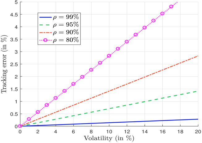
Figure 10: Relationship between volatility and tracking error levels

The previous result is of major importance, because it states that the tracking error level of the tactical portfolio must be related to the volatility of the strategic portfolio. In practice, the volatility is time-varying, implying that using a constant tracking error strategy is not optimal.

There is a second reason to consider a time-varying tracking error level, because another issue concerns the relationship between the tracking error and the active bets. We can show that (Grinold, 1994):

$$\mu\left(x\mid\tilde{x}\right)=\sigma\left(x\mid\tilde{x}\right)\cdot\mathop{\rm TC}\cdot\mathop{\rm IC}\cdot\sqrt{n}$$

where $\mathop{\rm TC}$ is the transfer coefficient, $\mathop{\rm IC}$ is the information coefficient and $n$ is the number of assets. This relationship is known as “the fundamental law of active management”. If we assume that $\mathop{\rm TC}$ and $\mathop{\rm IC}$ are constant for a given active manager and a given portfolio, it follows that the excess return is proportional to the tracking error volatility:

$$\mu\left(x\mid\tilde{x}\right)\propto\sigma\left(x\mid\tilde{x}\right)$$

However, alpha generation is also linked to the number and strength of active bets:

$$\mu\left(x\mid\tilde{x}\right)=g_{\mu}\left(s_{1},\ldots,s_{n}\right)$$

We deduce that the tracking error must be a function of the scores $s_{i}$:

$$\sigma\left(x\mid\tilde{x}\right)=g_{\sigma}\left(s_{1},\ldots,s_{n}\right)$$ (37)

This relationship is essential when considering tactical allocation. Indeed, if all the scores are equal to zero, there is no active bet, implying that we must target a zero tracking error level. If all the scores are equal, we are in the same situation. Indeed, since we are bullish in all the asset classes, there is no reason to deviate from the strategic portfolio. In order to take a high tracking error risk, we need the bets to present a high dispersion:

$$s_{i}$$ #1 #2 #3 #4

zero zero moderate high

Since the function $g_{\mu}$ is unknown and difficult to estimate, the function $g_{\sigma}$ is also unknown. However, we may use the following rule of thumb:

$$\sigma\left(x\mid\tilde{x}\right)\approx c\cdot\left(\frac{\sigma\left(s\right)+\mathop{\rm mad}\left(s\right)}{2}\right)\cdot\sigma^{+}$$ (38)

where $\sigma\left(s\right)$ is the standard deviation of scores, $\mathop{\rm mad}\left(s\right)$ is the mean absolute difference of scores, and $\sigma^{+}$ is the maximum tracking error. The value of $\sigma^{+}$ may be deduced from the relationship (36). By construction, we have:

$$0\leq\left(\frac{\sigma\left(s\right)+\mathop{\rm mad}\left(s\right)}{2}\right)\leq 3.6213$$

and:

$$0\leq\lim_{n\rightarrow\infty}\left(\frac{\sigma\left(s\right)+\mathop{\rm mad}\left(s\right)}{2}\right)\leq 3$$

where $n$ is the number of assets. It follows that the scaling factor $c$ is approximatively equal to $\dfrac{1}{3}$.

Equation (38) is a preliminary approach to set the level of tracking error. Nevertheless, this rule of thumb has a major drawback. It does not depend on the asset classes and their scores. Let us consider the previous example described on page 15. We assume that the signals are respectively $+$, $0$, $+$, $0$, $+$, $0$, $0$, $+$, $0$ and $+$. In Figure 11, we report the tactical allocation when we target a tracking error level. For Europe Equities, we have a signal equal to $+$, and we verify that the allocation is increasing with respect to the tracking error. For US Sovereign and IG Bonds, we also have a signal equal to $+$, but the relationship between the allocation and the tracking error is not monotonically increasing. The case of US IG Bonds will be easily solved once we consider Problem (4.2) instead of a simple tracking error optimization. The case of US Sovereign Bonds is more problematic. Indeed, in an initial period when the tracking error is low, the relationship is increasing. However, when the tracking error increases too much, we obtain the opposite result. The reason is that the volatility of US Sovereign Bonds is low compared to the other asset classes (equities, investment grade and high yield). If we increase the tracking error, there is a threshold beyond which it is better to play only active bets on the most risky assets. Indeed, playing active bets on low risk assets does not give rise to a high tracking error budget. This is why the optimizer switches from low-risk assets to high-risk assets. This means that the choice of a tracking error level depends on the set of parameters: the maximum tracking error that depends on the strategic portfolio, the scores or active bets and the volatility of the assets that compose the tactical portfolio.

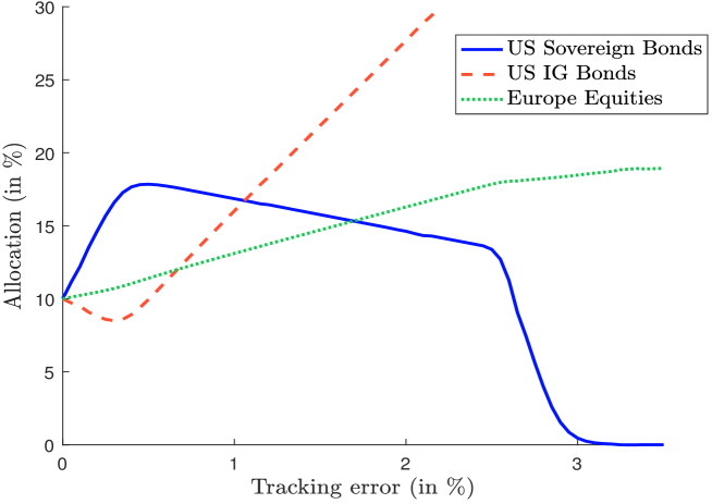
Figure 11: Relationship between active bets and tracking errors

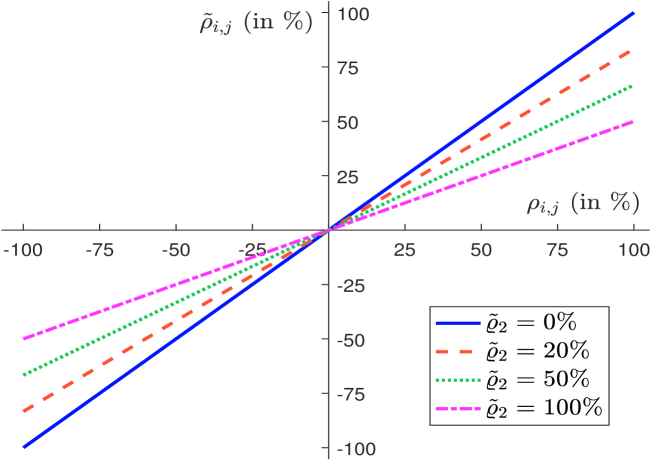
Figure 12: Impact of the ridge parameter on the shrinkage correlation

4.3.3 Calibrating the regularization parameters

As said previously, the choice of the regularization parameters is not straightforward and requires a solid expertise and experience. However, we will provide some tips that can help to calibrate the model. The first thing to notice concerns the magnitude of $\varrho_{1}$ and $\varrho_{2}$. On page 5, we have seen that if $\tilde{\Gamma}_{2}=\mathop{\rm diag}\Sigma$, the regularized correlations are:

$$\tilde{\rho}_{i,j}=\frac{\rho_{i,j}}{1+\tilde{\varrho}_{2}}$$

In Figure 12, we have reported the relationship between the initial correlation $\rho_{i,j}$ and the shrinkage correlation $\tilde{\rho}_{i,j}$. When $\tilde{\varrho}_{2}$ is equal to zero, $\tilde{\rho}_{i,j}=\rho_{i,j}$. When $\tilde{\varrho}_{2}\rightarrow\infty$, the shrinkage correlation tends to zero. We then obtain a diagonal matrix with equal volatilities. Therefore, there is a trade-off between considering the initial covariance matrix and ignoring the dependence between assets. A good way to choose $\tilde{\varrho}_{2}$ is to reduce the impact of arbitrage factors while keeping the significance of common risk factors. If we now consider the $L_{1}$ penalty $\varrho_{1}\left\|\Gamma_{1}\left(x-x_{t}\right)\right\|_{1}$ and if we set $\Gamma_{1}=I_{n}$, the $L_{1}$ norm measures the portfolio’s two-way turnover:

$$\left\|\left(x-x_{t}\right)\right\|_{1}=\sum_{i=1}^{n}\left|x_{i}-x_{i,t}\right|$$

The parameter $\varrho_{1}$ may then be used to control the turnover. If $\Gamma_{1}$ is a matrix with non-negative entries that contains the unit transaction costs, the $L_{1}$ norm measures the portfolio’s transaction cost (Scherer, 2007). This means that $\varrho_{1}$ is the average transaction cost if $\Gamma_{1}$ is the identity matrix. It follows that the order of magnitude of $\tilde{\varrho}_{2}$ is not comparable to the order of magnitude of $\varrho_{1}$. In the first case, it is expressed as a percentage (for instance, $\tilde{\varrho}_{2}=25\%$) whereas in the lasso problem it is expressed in basis points (for instance, $\varrho_{1}=5$ bps). This is in line with the practice that shows that optimal values of $L_{2}$ regularization are higher than those of $L_{1}$ regularization. The second thing to notice concerns the specification of regularization matrices $\Gamma_{1}$, $\tilde{\Gamma}_{1}$, $\Gamma_{2}$ and $\tilde{\Gamma}_{2}$. Most of the time, they correspond to diagonal matrices, because it is not easy to consider the cross effects of regularization. The simplest way is to consider identity matrices, meaning that the regularization patterns reduce to ridge and lasso approaches. If we use the same parameters $\varrho_{1}=\tilde{\varrho}_{1}$ and $\varrho_{2}=\tilde{\varrho}_{2}$, it is equivalent to considering that the two portfolios plays a symmetric role. However, this is not the case. Portfolio $x_{t}$ is used in order to limit the turnover and to smooth the dynamic allocation. Portfolio $\tilde{x}$ is used in order to control the relative active bets. This is why $\tilde{x}$ is more important than $x_{t}$ for implementing the active management. Last but not least, the calibration of the parameters highly depends on the investment profile. If the fund is composed of equities, we need to use more aggressive parameters in order to be more active than with a multi-asset fund. This means that there is no magic formula, and the calibration stage requires much empirical research and many tests in order to understand the interconnectedness between the different terms of the portfolio optimization problem.

5 Conclusion

According to Fisch et al. (2017), robo-advisors are “computer algorithms that provide advice on investment portfolios and then manage those portfolios”. Since they are digital-based tools that are generally implemented as web online services, fintechs compete in order to offer better customization, data visualization, analytics, process automation, etc. And the concepts of artificial intelligence, big data and machine learning are never far away when we see the presentation of a robo-advisor. Most of the time, fintechs prefer to insist on the application’s ergonomics and functionalities, and give little insight into the robo-advisor’s raison d’être: an automated portfolio allocation engine.

One of the reasons may be that portfolio allocation is more human-based than computer-based. It is true that automation in portfolio optimization is a big issue. Indeed, portfolio optimization is a hard task and does not always produce the desired results. This is because the mathematical problem is not necessarily well defined when we would like to obtain a smooth, sparse, active and dynamic allocation.

In this article, we come back to the traditional mean-variance optimization, and identify the reason for the issues. We have shown that it primarily corresponds to an alpha optimizer, and not to a beta optimizer. Then we have presented the theory of regularization and sparsity, and have demonstrated how it improves portfolio optimization. Finally, this approach is applied for building automated robo-advisory.

Appendix A Mathematical results

A.1 Notations

We use the following notations:

• $\mathds{1}_{\Omega}\left(x\right)$ is the convex indicator function of $\Omega$: $\mathds{1}_{\Omega}\left(x\right)=0$ for $x\in\Omega$ and $\mathds{1}_{\Omega}\left(x\right)=+\infty$ for $x\notin\Omega$.

• $A^{\dagger}$ is the Moore-Penrose pseudo-inverse matrix of $A$; in the scalar case, we have $0^{\dagger}=0$ and $a^{\dagger}=a^{-1}$ if $a\neq 0$.

• $\mathcal{C}=\left(\rho_{i,j}\right)$ denotes the correlation matrix with entries $\rho_{i,j}$.

• $\mathcal{C}_{n}\left(\rho\right)$ is the constant correlation matrix of dimension $n$, whose uniform correlation is $\rho$.

• $\mu$ is the vector of expected return.

• $\Sigma$ is the covariance matrix.

• $\left\|x\right\|_{p}=\left(\sum_{i=1}^{n}\left|x_{i}\right|^{p}\right)^{1/p}$ is the $L_{p}$ norm.

• $\left\|x\right\|_{A}=\left(x^{\top}Ax\right)^{1/2}$ is the weighted $L_{2}$ norm.

• $\left[M\right]_{i,j}$ is the $\left(i,j\right)$ entry of the matrix $M$.

• $x\odot y$ is the Hadamard element-wise product: $\left[x\odot y\right]_{i,j}=\left[x\right]_{i,j}\left[y\right]_{i,j}$.

• $\mathcal{P}_{\Omega}\left(x\right)$ is the projection of $x$ on the set $\Omega$:

  $$\mathcal{P}_{\Omega}\left(x\right)=\arg\min\nolimits_{y\in\Omega}\frac{1}{2}\left\|y-x\right\|_{2}^{2}$$

• $\mathbf{prox}_{f}\left(v\right)$ is the proximal operator of $f\left(x\right)$:

  $$\mathbf{prox}_{f}\left(v\right)=\arg\min\nolimits_{x}\left\{f\left(x\right)+\frac{1}{2}\left\|x-v\right\|_{2}^{2}\right\}$$

A.2 Matrix form of the estimators $\hat{\mu}$ and $\hat{\Sigma}$

Since we have $\hat{\mu}=\sum_{t=1}^{T}w_{t}R_{t}$, it follows that $\hat{\mu}=R^{\top}w$ where $w=\left(w_{1},\ldots,w_{T}\right)\in\mathbb{R}^{T}$ and $R=\left(R_{1},\ldots,R_{T}\right)\in\mathbb{R}^{T\times n}$. By noting $D_{w}=\mathop{\rm diag}\left(w\right)$, the expression of the covariance matrix becomes:

$$\hat{\Sigma} = \sum_{t=1}^{T}w_{t}R_{t}R_{t}^{\top}-\hat{\mu}\hat{\mu}^{\top}$$

$$= \sum_{t=1}^{T}w_{t}R_{t}R_{t}^{\top}-\left(\sum_{t=1}^{T}w_{t}R_{t}\right)\left(\sum_{t=1}^{T}w_{t}R_{t}\right)^{\top}$$

$$= R^{\top}D_{w}R-R^{\top}w\left(R^{\top}w\right)^{\top}$$

$$= R^{\top}\left(D_{w}-ww^{\top}\right)R$$

An alternative form is:

$$\hat{\Sigma} = \sum_{t=1}^{T}w_{t}\left(R_{t}-\hat{\mu}\right)\left(R_{t}-\hat{\mu}\right)^{\top}$$

$$= \left(R-\mathbf{1}\hat{\mu}^{\top}\right)^{\top}D_{w}\left(R-\mathbf{1}\hat{\mu}^{\top}\right)$$

$$= \left(R-\mathbf{1}w^{\top}R\right)^{\top}D_{w}\left(R-\mathbf{1}w^{\top}R\right)$$

$$= R^{\top}\left(C_{T}^{\top}D_{w}C_{T}\right)R$$

where $C_{T}=I_{T}-\mathbf{1}w^{\top}$ is the (weighted) centering matrix. In the case of uniform weights $w_{t}=1/T$, $C_{T}$ is equal to $I_{T}-\dfrac{1}{T}\mathbf{11}^{\top}$. We observe that it is symmetric and idempotent. We deduce that $\hat{\Sigma}=\dfrac{1}{T}R^{\top}C_{T}R$.

A.3 Relationship between the conditional normal distribution and the linear regression

Let us consider a Gaussian random vector defined as follows:

$$\left(\begin{array}[]{c}X\\ Y\end{array}\right)\sim\mathcal{N}\left(\left(\begin{array}[]{c}\mu_{x}\\ \mu_{y}\end{array}\right),\left(\begin{array}[]{cc}\Sigma_{xx}&\Sigma_{xy}\\ \Sigma_{yx}&\Sigma_{yy}\end{array}\right)\right)$$

The conditional distribution of $Y$ given $X=x$ is a multivariate normal distribution:

$$Y\mid X=x\sim\mathcal{N}\left(\mu_{y\mid x},\Sigma_{yy\mid x}\right)$$

where:

$$\mu_{y\mid x}=\mathbb{E}\left[Y\mid X=x\right]=\mu_{y}+\Sigma_{yx}\Sigma_{xx}^{-1}\left(x-\mu_{x}\right)$$

and:

$$\Sigma_{yy\mid x}=\sigma^{2}\left[Y\mid X=x\right]=\Sigma_{yy}-\Sigma_{yx}\Sigma_{xx}^{-1}\Sigma_{xy}$$

It follows that $Y=\mu_{y\mid x}+U$ where $U$ is a centered Gaussian random variable with variance $s^{2}=\Sigma_{yy\mid x}$.We recognize the linear regression of $Y$ on $X$:

$$Y = \mu_{y}+\Sigma_{yx}\Sigma_{xx}^{-1}\left(x-\mu_{x}\right)+U$$

$$= \left(\mu_{y}-\Sigma_{yx}\Sigma_{xx}^{-1}\mu_{x}\right)+\Sigma_{yx}\Sigma_{xx}^{-1}x+U$$

$$= \alpha+\beta^{\top}x+U$$

where $\alpha=\mu_{y}-\Sigma_{yx}\Sigma_{xx}^{-1}\mu_{x}$ and $\beta=\Sigma_{yx}\Sigma_{xx}^{-1}$. Moreover, we have:

$$\mathfrak{R}^{2} = 1-\frac{\mathop{\rm var}\left(U\right)}{\mathop{\rm var}\left(Y\right)}$$

$$= 1-\frac{s^{2}}{\Sigma_{yy}}$$

$$= \frac{\Sigma_{yx}\Sigma_{xx}^{-1}\Sigma_{xy}}{\Sigma_{yy}}$$

Remark 7

In the case where the correlation matrix of the random vector $\left(X,Y\right)$ is constant – $\mathcal{C}=\mathcal{C}_{n+1}\left(\rho\right)$, Maillard et al. (2010) proved that:

$$\mathcal{C}_{xx}^{-1}=\frac{\rho\mathbf{11}^{\top}-\left(\left(n-1\right)\rho+1\right)I_{n}}{\left(n-1\right)\rho^{2}-\left(n-2\right)\rho-1}$$

We deduce that:

$$\beta = \Sigma_{xx}^{-1}\Sigma_{xy}$$

$$= \left(\frac{\sigma_{x}}{\sigma_{y}}\right)\odot\mathcal{C}_{xx}^{-1}\mathcal{C}_{x,y}$$

$$= \left(\frac{\sigma_{x}}{\sigma_{y}}\right)\odot\left(\frac{\rho\mathbf{11}^{\top}-\left(\left(n-1\right)\rho+1\right)I_{n}}{\left(n-1\right)\rho^{2}-\left(n-2\right)\rho-1}\right)\rho\mathbf{1}$$

and:

$$\beta_{i}=\frac{\rho\left(\rho-1\right)}{\left(n-1\right)\rho^{2}-\left(n-2\right)\rho-1}\cdot\frac{\sigma_{y}}{\sigma_{x_{i}}}$$

where $\sigma_{y}$ and $\sigma_{x}$ are the standard deviation of random vectors $Y$ and $X$. The coefficient of determination becomes:

$$\mathfrak{R}^{2} = \frac{\Sigma_{yx}\Sigma_{xx}^{-1}\Sigma_{xy}}{\Sigma_{yy}}$$

$$= \frac{n\rho^{2}}{n\rho-\left(\rho-1\right)}$$

In the two-asset case, we obtain the famous result: $\mathfrak{R}^{2}=\rho^{2}$. When the number of assets is very large, the coefficient of determination is equal to the uniform correlation:

$$\lim_{n\rightarrow\infty}\mathfrak{R}^{2}=\left\{\begin{array}[]{ll}1&\text{if }\rho<0\\ \rho&\text{if }\rho\geqslant 0\end{array}\right.$$

A.4 Tikhonov regularization

We consider the following optimization problem:

$$x^{\star} = \arg\min\frac{1}{2}\left\|A_{1}x-b_{1}\right\|_{2}^{2}+\frac{1}{2}\varrho_{2}\left\|\Gamma_{2}\left(x-x_{0}\right)\right\|_{2}^{2}$$

s.t. $$A_{2}x=b_{2}$$

where $A_{1}\in\mathbb{R}^{T\times n}$, $b_{1}\in\mathbb{R}^{T\times 1}$, $\varrho_{2}>0$, $\Gamma\in\mathbb{R}^{n\times n}$, $A_{2}\in\mathbb{R}^{m\times n}$, $b_{2}\in\mathbb{R}^{m\times 1}$ and $d\in\mathbb{R}^{m\times 1}$. We assume that $A_{1}$ has full rank. The Tikhonov matrix $\Gamma_{2}$ forces desirable properties of the solution whereas $\varrho_{2}$ indicates the strength of the regularization. $x_{0}$ is an initial solution. In the case of portfolio optimization, it could be an heuristic portfolio (like the EW portfolio) or the current allocation in order to control the turnover (Scherer, 2007). The Lagrange function is equal to:

$$\mathcal{L}\left(x,\lambda\right)=\frac{1}{2}\left\|A_{1}x-b_{1}\right\|_{2}^{2}+\frac{1}{2}\varrho_{2}\left\|\Gamma_{2}\left(x-x_{0}\right)\right\|_{2}^{2}+\lambda^{\top}\left(A_{2}x-b_{2}\right)$$

Computation of the gradient leads to:

$$\partial_{x}\,\mathcal{L}\left(x,\lambda\right)=A_{1}^{\top}\left(A_{1}x-b_{1}\right)+\varrho_{2}\Gamma_{2}^{\top}\Gamma_{2}\left(x-x_{0}\right)+A_{2}^{\top}\lambda$$

Since we have $\partial_{x}\,\mathcal{L}\left(x,\lambda\right)=\mathbf{0}$ and $A_{2}x=b_{2}$, the optimal portfolio $x^{\star}$ is the $x$-coordinate solution of the linear system:

$$\left(\begin{array}[]{cc}A_{1}^{\top}A_{1}+\varrho_{2}\Gamma_{2}^{\top}\Gamma_{2}&A_{2}^{\top}\\ A_{2}&\mathbf{0}\end{array}\right)\left(\begin{array}[]{c}x\\ \lambda\end{array}\right)=\left(\begin{array}[]{c}A_{1}^{\top}b_{1}+\varrho_{2}\Gamma_{2}^{\top}\Gamma_{2}x_{0}\\ b_{2}\end{array}\right)$$ (40)

This linear system gives the primal and dual variables.

A.5 Limit solutions of $L_{p}$ - $L_{2}$ regularization

As $\varrho_{p}$ is fixed and $\varrho_{2}$ tends to $+\infty$, the formal limit to Problem (3.5.2) is given by:

$$x^{\star}=\arg\min\left\|\Gamma_{2}\left(x-x_{0}\right)\right\|_{2}^{2}\quad\text{s.t.}\quad A_{2}x=b_{2}$$

As $\varrho_{2}$ is fixed and $\varrho_{p}$ tends to $+\infty$, the formal limit to Problem (3.5.2) is given by:

$$x^{\star}=\arg\min\left\|\Gamma_{p}\left(x-x_{0}\right)\right\|_{p}^{p}\quad\text{s.t.}\quad A_{2}x=b_{2}$$

If $\varrho_{p}$ and $\varrho_{2}$ both tend to $+\infty$, the formal limit to Problem (3.5.2) depends on the regime $\varrho_{p}/\varrho_{2}$.

A.6 Augmented QP algorithm

A quadratic programming (QP) problem is an optimization problem with a quadratic objective function and linear constraints:

$$x^{\star} = \arg\min\frac{1}{2}x^{\top}A_{1}x-x^{\top}b_{1}$$

s.t. $$A_{3}x\geqslant b_{3}$$

With the inequality constraints, we can easily manage equality constraints and bounds. If we introduce a $L_{2}$ penalization, the optimization program becomes:

$$\left(\ast\right) = \frac{1}{2}x^{\top}A_{1}x-x^{\top}b_{1}+\frac{1}{2}\varrho_{2}\left\|\Gamma_{2}\left(x-x_{0}\right)\right\|_{2}^{2}$$

$$= \frac{1}{2}x^{\top}A_{1}x-x^{\top}b_{1}+\frac{1}{2}\varrho_{2}x^{\top}\Gamma_{2}x-\varrho_{2}x^{\top}\Gamma_{2}x_{0}+\frac{1}{2}\varrho_{2}x_{0}^{\top}\Gamma_{2}x_{0}$$

We deduce that the regularization program can be cast into a QP problem:

$$x^{\star} = \arg\min\frac{1}{2}x^{\top}A_{1}\left(\varrho_{2}\right)x-x^{\top}b_{1}\left(\varrho_{2}\right)$$

s.t. $$A_{3}x\geqslant b_{3}$$

where $A_{1}\left(\varrho_{2}\right)=A_{1}+\varrho_{2}\Gamma_{2}$ and $b_{1}\left(\varrho_{2}\right)=b_{1}+\varrho_{2}\Gamma_{2}x_{0}$.

Let us now introduce an $L_{1}$ penalization. We have:

$$x^{\star} = \arg\min f\left(x\right)$$

s.t. $$A_{3}x\geqslant b_{3}$$

where:

$$f\left(x\right)=\frac{1}{2}x^{\top}A_{1}x-x^{\top}b_{1}+\varrho_{1}\left\|\Gamma_{1}\left(x-x_{0}\right)\right\|_{1}$$

and $\Gamma_{1}$ is a matrix with non-negative entries. If we use a decomposition of the following form:

$$x=x_{0}+\delta^{+}-\delta^{-}$$ (43)

with $\delta^{-}=\left(\delta_{1}^{-},\ldots,\delta_{n}^{-}\right)$, $\delta^{+}=\left(\delta_{1}^{+},\ldots,\delta_{n}^{+}\right)$, $\delta_{i}^{-}\geqslant 0$ and $\delta_{i}^{+}\geqslant 0$, we deduce that:

$$\left\|\Gamma_{1}\left(x-x_{0}\right)\right\|_{1}=\left\|\Gamma_{1}\left(\delta^{+}-\delta^{-}\right)\right\|_{1}=\mathbf{1}^{\top}\left(\Gamma_{1}\left(\delta^{+}+\delta^{-}\right)\right)$$

The objective function becomes:

$$f\left(x\right)=\frac{1}{2}x^{\top}A_{1}x-x^{\top}b_{1}+\mathbf{1}^{\top}\Gamma_{1}\delta^{+}+\mathbf{1}^{\top}\Gamma_{1}\delta^{-}$$

Let $y=\left(x,\delta^{-},\delta^{+}\right)$ be the vector of unknown variables. We obtain an augmented QP problem of dimension $3\times n$:

$$y^{\star} = \arg\min\frac{1}{2}y^{\top}\tilde{A}_{1}y-y^{\top}\tilde{b}_{1}$$

s.t. $$\tilde{A}_{3}y\geqslant\tilde{b}_{3}$$

where:

$$\tilde{A}_{1}=\left(\begin{array}[]{ccc}A_{1}&\mathbf{0}&\mathbf{0}\\ \mathbf{0}&\mathbf{0}&\mathbf{0}\\ \mathbf{0}&\mathbf{0}&\mathbf{0}\end{array}\right)$$

and:

$$\tilde{b}_{1}=\left(\begin{array}[]{c}b_{1}\\ -\Gamma_{1}^{\top}\mathbf{1}\\ -\Gamma_{1}^{\top}\mathbf{1}\end{array}\right)$$

We can write Equation (43) as follows:

$$I_{n}x+I_{n}\delta^{-}-I_{n}\delta^{+}=x_{0}$$

Since we have $\delta^{+}\geqslant\mathbf{0}$ and $\delta^{-}\geqslant\mathbf{0}$, we deduce that:

$$\tilde{A}_{3}=\left(\begin{array}[]{rrr}A_{3}&\mathbf{0}&\mathbf{0}\\ I_{n}&I_{n}&-I_{n}\\ -I_{n}&-I_{n}&I_{n}\\ \mathbf{0}&I_{n}&\mathbf{0}\\ \mathbf{0}&\mathbf{0}&I_{n}\end{array}\right)$$

and:

$$\tilde{b}_{3}=\left(\begin{array}[]{r}b_{3}\\ x_{0}\\ -x_{0}\\ \mathbf{0}\\ \mathbf{0}\end{array}\right)$$

A.7 ADMM algorithm

A.7.1 Dual ascent principle and method of multipliers

The alternating direction method of multipliers (ADMM) is an algorithm introduced by Gabay and Mercier (1976) to solve problems which can be expressed as:

$$\left\{x^{\star},z^{\star}\right\} = \arg\min f\left(x\right)+g\left(z\right)$$

s.t. $$Ax+Bz=c$$

where $A\in\mathbb{R}^{p\times n}$, $B\in\mathbb{R}^{p\times m}$, $c\in\mathbb{R}^{p}$, and the functions $f:\mathbb{R}^{n}\rightarrow\mathbb{R}\cup\{+\infty\}$ and $g:\mathbb{R}^{m}\rightarrow\mathbb{R}\cup\{+\infty\}$ are proper closed convex functions. The expression of the augmented Lagrange function is:

$$\mathcal{L}_{\varphi}\left(x,z,\lambda\right)=f\left(x\right)+g\left(z\right)+\lambda^{\top}\left(Ax+Bz-c\right)+\frac{\varphi}{2}\left\|Ax+Bz-c\right\|_{2}^{2}$$

where $\varphi>0$. The ADMM algorithm uses the property that the objective function is separable, and consists of the following iterations:

$$x^{\left(k+1\right)} = \arg\min\mathcal{L}_{\varphi}\left(x,z^{\left(k\right)},\lambda^{\left(k\right)}\right)$$

$$= \arg\min\left\{f\left(x\right)+\lambda^{\left(k\right)^{\top}}\left(Ax+Bz^{\left(k\right)}-c\right)+\frac{\varphi}{2}\left\|Ax+Bz^{\left(k\right)}-c\right\|_{2}^{2}\right\}$$

and:

$$z^{\left(k+1\right)} = \arg\min\mathcal{L}_{\varphi}\left(x^{\left(k+1\right)},z,\lambda^{\left(k\right)}\right)$$

$$= \arg\min\left\{g\left(z\right)+\lambda^{\left(k\right)^{\top}}\left(Ax^{\left(k+1\right)}+Bz-c\right)+\frac{\varphi}{2}\left\|Ax^{\left(k+1\right)}+Bz-c\right\|_{2}^{2}\right\}$$

The update for the dual variable $\lambda$ is then:

$$\lambda^{\left(k+1\right)}=\lambda^{\left(k\right)}+\varphi\left(Ax^{\left(k+1\right)}+Bz^{\left(k+1\right)}-c\right)$$

We repeat the iterations until convergence.

Boyd et al. (2011) notice that the previous algorithm can be simplified. Let $r=Ax+Bz-c$ be the (primal) residual. By combining linear and quadratic terms, we have:

$$\lambda^{\top}r+\frac{\varphi}{2}r^{2}=\frac{\varphi}{2}\left\|r+u\right\|^{2}-\frac{\varphi}{2}\left\|u\right\|^{2}$$

where $u=\varphi^{-1}\lambda$ is the scaled dual variable. We can then write the Lagrange function (A.7.1) as follows:

$$\mathcal{L}_{\varphi}\left(x,z,u\right)=f\left(x\right)+g\left(z\right)+\frac{\varphi}{2}\left\|Ax+Bz-c+u\right\|_{2}^{2}-\frac{1}{2\varphi}\left\|\lambda\right\|^{2}$$ (46)

Since the last term is a constant, we deduce that the $x$- and $z$-updates become:

$$x^{\left(k+1\right)} = \arg\min\mathcal{L}_{\varphi}\left(x,z^{\left(k\right)},u^{\left(k\right)}\right)$$ (47)

$$= \arg\min\left\{f\left(x\right)+\frac{\varphi}{2}\left\|Ax+Bz^{\left(k\right)}-c+u^{\left(k\right)}\right\|_{2}^{2}\right\}$$

and:

$$z^{\left(k+1\right)} = \arg\min\mathcal{L}_{\varphi}\left(x^{\left(k+1\right)},z,u^{\left(k\right)}\right)$$ (48)

$$= \arg\min\left\{g\left(z\right)+\frac{\varphi}{2}\left\|Ax^{\left(k+1\right)}+Bz-c+u^{\left(k\right)}\right\|_{2}^{2}\right\}$$

For the scaled dual variable $u^{\left(k\right)}$, we have:

$$u^{\left(k+1\right)} = u^{\left(k\right)}+r^{\left(k+1\right)}$$ (49)

$$= u^{\left(k\right)}+\left(Ax^{\left(k+1\right)}+Bz^{\left(k+1\right)}-c\right)$$

where $r^{\left(k+1\right)}=Ax^{\left(k+1\right)}+Bz^{\left(k+1\right)}-c$ is the primal residual at iteration $k+1$. Boyd et al. (2011) also defined the variable $s^{\left(k+1\right)}=\varphi A^{\top}B\left(z^{\left(k+1\right)}-z^{\left(k\right)}\right)$ and refer to $s^{\left(k+1\right)}$ as the dual residual at iteration $k+1$.

This algorithm benefits from the dual ascent principle and the method of multipliers. The difference with the latter is that the $x$ and $z$-updates are performed in an alternating way. Therefore, it is more flexible because the updates are equivalent to compute proximal operators for $f$ and $g$, independently.

A.7.2 Convergence and stopping criteria

Under the assumption that the traditional Lagrange function $\mathcal{L}_{0}$ has a saddle point, one can prove that the residual $r^{\left(k\right)}$ converges to zero, the objective function $f\left(x^{\left(k\right)}\right)+g\left(z^{\left(k\right)}\right)$ to the optimal value $f\left(x^{\star}\right)+g\left(z^{\star}\right),$ and the dual variable $\lambda^{\left(k\right)}$ to a dual optimal point. However, the rate of convergence is not known and the primal variables $x^{\left(k\right)}$ and $z^{\left(k\right)}$ do not necessarily converge to the optimal values $x^{\star}$ and $z^{\star}$. Nevertheless, in the context of Markowitz optimization with bound constraints, the results found by Raghunathan and Di Cairano (2014) may be applied to obtain linear convergence for the primal variables.

In general, the stopping criterion is defined with respect to the residuals:

$$\left\{\begin{array}[]{l}\left\|r^{\left(k\right)}\right\|_{2}\leqslant\varepsilon\\ \left\|s^{\left(k\right)}\right\|_{2}\leqslant\varepsilon^{\prime}\end{array}\right.$$

where $r^{\left(k\right)}=Ax^{\left(k\right)}+Bz^{\left(k\right)}-c$ and $s^{\left(k\right)}=\varphi A^{\top}B\left(z^{\left(k\right)}-z^{\left(k-1\right)}\right)$. Typical values when implementing this stopping criterion are $\varepsilon=\varepsilon^{\prime}=10^{-18}$.

A.7.3 Penalization parameter and initialization

The convergence result holds regardless of the choice of the penalization parameter $\varphi>0$. But the choice of $\varphi$ affects the speed of convergence (Ghadimi et al., 2015; Giselsson and Boyd, 2017). In practice, the penalization parameter $\varphi$ may be changed at each iteration, implying that $\varphi$ is replaced by $\varphi^{\left(k\right)}$ and the scaled dual variable $u^{k}$ is equal to $\lambda^{\left(k\right)}/\varphi^{\left(k\right)}$. This may improve the convergence and make the performance independent of the initial choice $\varphi^{\left(0\right)}$. To update $\varphi^{\left(k\right)}$ in practice, He et al. (2000) and Wang and Liao (2001) provide a simple and efficient scheme. On the one hand, the $x$ and $z$-updates in ADMM essentially comes from placing a penalty on $\left\|r^{\left(k\right)}\right\|_{2}^{2}$. As a consequence, if $\varphi^{\left(k\right)}$ is large, $\left\|r^{\left(k\right)}\right\|_{2}^{2}$ tends to be small. On the other hand, $s^{\left(k\right)}$ depends linearly on $\varphi$. As a consequence, if $\varphi^{\left(k\right)}$ is small, $\left\|s^{\left(k\right)}\right\|_{2}^{2}$ is small (and $\left\|r^{\left(k\right)}\right\|_{2}^{2}$ may be large). To keep $\left\|r^{\left(k\right)}\right\|_{2}^{2}$ and $\left\|s^{\left(k\right)}\right\|_{2}^{2}$ within a factor $\mu$, one may consider:

$$\varphi^{\left(k+1\right)}=\left\{\begin{array}[]{ll}\tau\varphi^{\left(k\right)}&\text{if }\left\|r^{\left(k\right)}\right\|_{2}^{2}>\mu\left\|s^{\left(k\right)}\right\|_{2}^{2}\\ \varphi^{\left(k\right)}/\tau^{\prime}&\text{if }\left\|s^{\left(k\right)}\right\|_{2}^{2}>\mu\left\|r^{\left(k\right)}\right\|_{2}^{2}\\ \varphi^{\left(k\right)}&\text{otherwise}\end{array}\right.$$

where $\mu$, $\tau$ and $\tau^{\prime}$ are parameters that are greater than one. In practice, we use $\varphi^{\left(0\right)}=1$, $u^{\left(0\right)}=0$, $\mu=10^{3}$ and $\tau=\tau^{\prime}=2$.

A.7.4 Tikhonov regularization

Let us consider the Tikhonov problem:

$$x^{\star} = \arg\min\frac{1}{2}\left\|A_{1}x-b_{1}\right\|_{2}^{2}+\frac{1}{2}\varrho_{2}\left\|\Gamma_{2}\left(x-x_{0}\right)\right\|_{2}^{2}$$ (50)

$$s.t. \left\{\begin{array}[]{l}\left\|x\right\|_{q}\leqslant c_{q}\\ A_{2}x=b_{2}\\ A_{3}x\leqslant b_{3}\\ x^{-}\leqslant x\leqslant x^{+}\end{array}\right.$$ (55)

where $q\in[1,\infty)$. We note:

$$\Omega_{1} = \left\{x\in\mathbb{R}^{n}:\left\|x\right\|_{q}\leqslant c_{q}\right\}$$

$$\Omega_{2} = \left\{x\in\mathbb{R}^{n}:A_{2}x=b_{2}\right\}$$

$$\Omega_{3} = \left\{x\in\mathbb{R}^{n}:A_{3}x\geqslant b_{3}\right\}$$

$$\Omega_{4} = \left\{x\in\mathbb{R}^{n}:x^{-}\leqslant x\leqslant x^{+}\right\}$$

We define:

$$f\left(x\right)=\frac{1}{2}\left\|A_{1}x-b_{1}\right\|_{2}^{2}+\frac{1}{2}\varrho_{2}\left\|\Gamma_{2}\left(x-x_{0}\right)\right\|_{2}^{2}+\mathbf{1}_{\Omega_{2}}\left(x\right)$$

and:

$$g\left(x\right)=\mathbf{1}_{\Omega_{1}}\left(x\right)+\mathbf{1}_{\Omega_{3}}\left(x\right)+\mathbf{1}_{\Omega_{4}}\left(x\right)$$

The Tikhonov problem becomes:

$$\left\{x^{\star},z^{\star}\right\} = \arg\min f\left(x\right)+g\left(z\right)$$

s.t. $$x-z=\mathbf{0}$$

Therefore, the ADMM algorithm is:

$$x^{\left(k+1\right)} = \arg\min\left\{f\left(x\right)+\frac{\varphi^{\left(k\right)}}{2}\left\|x-z^{\left(k\right)}+u^{\left(k\right)}\right\|_{2}^{2}\right\}$$

$$z^{\left(k+1\right)} = \arg\min\left\{g\left(z\right)+\frac{\varphi^{\left(k\right)}}{2}\left\|x^{\left(k+1\right)}-z+u^{\left(k\right)}\right\|_{2}^{2}\right\}$$

$$u^{\left(k+1\right)} = u^{\left(k\right)}+\left(x^{\left(k+1\right)}-z^{\left(k+1\right)}\right)$$

We notice that we can replace the second step by:

$$z^{\left(k+1\right)}=\mathcal{P}_{\left\{g\left(z\right)<\infty\right\}}\left(x^{\left(k+1\right)}+u^{\left(k\right)}\right)$$

where $\mathcal{P}_{\left\{g\left(z\right)<\infty\right\}}\left(x^{\left(k+1\right)}+u^{\left(k\right)}\right)$ is the orthogonal projection of $x^{\left(k+1\right)}+u^{\left(k\right)}$ onto the convex set $\left\{z\in\mathbb{R}^{n}:g\left(z\right)<\infty\right\}$.With this formulation, the $x$-step is explicit, while the $z$-step consists in computing orthogonal projections onto a convex set. Explicit formulas for orthogonal projections are presented in Appendix A.8 on page A.8.

A.7.5 Mixed regularization

We now replace the objective function of the Tikhonov problem by:

$$x^{\star}=\arg\min\frac{1}{2}\left\|A_{1}x-b_{1}\right\|_{2}^{2}+\frac{1}{2}\varrho_{2}\left\|\Gamma_{2}\left(x-x_{0}\right)\right\|_{2}^{2}+\frac{1}{p}\varrho_{p}\left\|\Gamma_{p}\left(x-x_{0}\right)\right\|_{p}^{p}$$ (56)

where $p\neq 2$. The constraints are the same than those specified for the Tikhonov problem. We define:

$$f\left(x\right) = \frac{1}{2}\left\|A_{1}x-b_{1}\right\|_{2}^{2}+\frac{1}{2}\varrho_{2}\left\|\Gamma_{2}\left(x-x_{0}\right)\right\|_{2}^{2}+$$

$$\mathbf{1}_{\Omega_{1}}\left(x\right)+\mathbf{1}_{\Omega_{2}}\left(x\right)+\mathbf{1}_{\Omega_{3}}\left(x\right)+\mathbf{1}_{\Omega_{4}}\left(x\right)$$

and:

$$g\left(z\right)=\frac{1}{p}\varrho_{p}\left\|z\right\|_{p}^{p}$$

The $L_{2}-L_{p}$ problem becomes:

$$\left\{x^{\star},z^{\star}\right\} = \arg\min f\left(x\right)+g\left(z\right)$$

s.t. $$\Gamma_{p}\left(x-x_{0}\right)-z=\mathbf{0}$$

With this specification, the ADMM algorithm is:

$$x^{\left(k+1\right)} = \arg\min\left\{f\left(x\right)+\frac{\varphi^{\left(k\right)}}{2}\left\|\Gamma_{p}x-z^{\left(k\right)}-\Gamma_{p}x_{0}+u^{\left(k\right)}\right\|_{2}^{2}\right\}$$

$$z^{\left(k+1\right)} = \arg\min\left\{g\left(z\right)+\frac{\varphi^{\left(k\right)}}{2}\left\|\Gamma_{p}x^{\left(k+1\right)}-z-\Gamma_{p}x_{0}+u^{\left(k\right)}\right\|_{2}^{2}\right\}$$

$$u^{\left(k+1\right)} = u^{\left(k\right)}+\left(\Gamma_{p}x^{\left(k+1\right)}-z^{\left(k+1\right)}-\Gamma_{p}x_{0}\right)$$

The $x$-step consists in minimizing a quadratic constrained problem. It can be carried out explicitly if no inequality constraint is imposed. Otherwise, the $x$-step can be performed by another ADMM. The $z$-step consists in computing the proximal operator of $\lambda\left\|z\right\|_{p}^{p}$ at the point $z=\Gamma_{p}x^{\left(k+1\right)}-\Gamma_{p}x_{0}+u^{\left(k\right)}$ with $\lambda=\varrho_{p}/\left(p\varphi^{\left(k\right)}\right)$. Other choices for the functions $f\left(x\right)$ and $g\left(z\right)$ give rise to computing constrained proximal operators or the proximal operator of $x\mapsto\left\|\Gamma_{p}x\right\|_{p}^{p}$. No explicit formula is known for the latter, unless a positive multiple of $\Gamma_{p}$ is orthogonal (Beck, 2017). Our choice makes the $z$-step explicit for $p\in\left\{1,2,3,4,5\right\}$, and easily computable for any $p>1$.

A.7.6 Cardinality constraints

The ADMM algorithm can also be used to find a portfolio with at most $n_{1}$ non-zero weights. Let us introduce the set $\mathcal{Z}$ of $n_{1}$-sparse vectors:

$$\mathcal{Z}=\left\{x\in\mathbb{R}^{n}\mid\mathop{\rm card}x\leqslant n_{1},x^{-}\leqslant x\leqslant x^{+}\right\}$$ (57)

We consider the augmented Tikohnov problem:

$$x^{\star} = \arg\min\frac{1}{2}\left\|A_{1}x-b_{1}\right\|_{2}^{2}+\frac{1}{2}\varrho_{2}\left\|\Gamma_{2}\left(x-x_{0}\right)\right\|_{2}^{2}$$ (58)

s.t. $$\left\{\begin{array}[]{l}x\in\Omega_{1}\cap\Omega_{2}\cap\Omega_{3}\cap\Omega_{4}\\ \Gamma_{1}\left(x-x_{0}\right)\in\mathcal{Z}\end{array}\right.$$ (61)

Zou and Hastie (2005) have been introduced Problem (56) with $p=1$ as a convex relaxation to problem (58). The constraint $x\in\mathcal{Z}$ is forced by the penalty $\varrho_{1}\left\|\Gamma_{1}\left(x-x_{0}\right)\right\|_{1}$ and the strength of the penalty parameter $\varrho_{1}$ must be chosen as the smallest value that satisfies the constraint $\mathop{\rm card}x\leqslant n_{1}$ (Hastie et al., 2009).

The projection onto the non-convex set $\mathcal{Z}$ exists and is explicit (but may not be unique). Diamond et al. (2018) show that:

$$\mathcal{P}_{\mathcal{Z}}\left(v\right)=\mathcal{P}_{\Omega_{4}}\left(v\left(n_{1}\right)\right)$$

where $v\left(n_{1}\right)_{i}=v_{i}$ if $i\in\mathcal{I}$, $v\left(n_{1}\right)_{i}=0$ if $i\not\in\mathcal{I}$, $\mathcal{I}$ is a set of indices of the $n_{1}$ largest values of $\left|v_{i}\right|$, and $\mathcal{P}_{\Omega_{4}}$ is the projection onto $\Omega_{4}=\left\{x\in\mathbb{R}^{n}:x^{-}\leqslant x\leqslant x^{+}\right\}$. As previously, we have:

$$f\left(x\right) = \frac{1}{2}\left\|A_{1}x-b_{1}\right\|_{2}^{2}+\frac{1}{2}\varrho_{2}\left\|\Gamma_{2}\left(x-x_{0}\right)\right\|_{2}^{2}+$$

$$\mathbf{1}_{\Omega_{1}}\left(x\right)+\mathbf{1}_{\Omega_{2}}\left(x\right)+\mathbf{1}_{\Omega_{3}}\left(x\right)+\mathbf{1}_{\Omega_{4}}\left(x\right)$$

and:

$$g\left(z\right)=\mathbf{1}_{\mathcal{Z}}\left(z\right)$$

with the constraint $\Gamma_{1}\left(x-x_{0}\right)=z$. With this specification, the ADMM algorithm is:

$$x^{\left(k+1\right)} = \arg\min\left\{f\left(x\right)+\frac{\varphi^{\left(k\right)}}{2}\left\|\Gamma_{p}x-z^{\left(k\right)}-\Gamma_{p}x_{0}+u^{\left(k\right)}\right\|_{2}^{2}\right\}$$

$$z^{\left(k+1\right)} = \mathcal{P}_{\mathcal{Z}}\left(\Gamma_{1}x^{\left(k+1\right)}-\Gamma_{1}x_{0}+u^{\left(k\right)}\right)$$

$$u^{\left(k+1\right)} = u^{\left(k\right)}+\left(\Gamma_{1}x^{\left(k+1\right)}-z^{\left(k+1\right)}-\Gamma_{1}x_{0}\right)$$

Hence, the $z$-step is explicit. The ADMM does not necessarily converge, and when it does, it does not necessarily converge to an optimal point. Contrary to the convex case, the possible convergence of the algorithm depends on the initial values of $x^{0}$ and the penalization parameter $\varphi^{\left(k\right)}$. In the non-convex setting, the ADMM may be considered as a local optimization method, and local neighbor search method with convex relaxation and restrictions may be used to obtain the convergence of the algorithm (Diamond et al., 2018).

A.8 Proximal operators and projections

As shown previously, the $z$-step of the ADMM algorithm generally computes the proximal operator of a norm or the projection onto the intersection of simple convex sets. We review the most useful cases in active asset management and we refer the reader to Parikh and Boyd (2014), Beck (2017), and Combettes and Müller (2018) for further examples. In most of these cases, the proximal operators are explicit or consists in determining the zero of a real-valued function.

A.8.1 Definition of the proximal operator

Let $f:\mathbb{R}^{n}\rightarrow\mathbb{R}\cup\left\{+\infty\right\}$ be a proper closed convex function. The proximal operator $\mathbf{prox}_{f}\left(v\right):\mathbb{R}^{n}\rightarrow\mathbb{R}^{n}$ is defined by:

$$\mathbf{prox}_{f}\left(v\right)=x^{\star}=\arg\min\nolimits_{x}\left\{f\left(x\right)+\frac{1}{2}\left\|x-v\right\|_{2}^{2}\right\}$$ (62)

Since the function $f_{v}\left(x\right)=f\left(x\right)+\dfrac{1}{2}\left\|x-v\right\|_{2}^{2}$ is strongly convex, it has a unique minimum for every $v\in\mathbb{R}^{n}$ (Beck, 2017; Parikh and Boyd, 2014).

If we would like to compute the proximal operator of $\lambda f\left(x\right)+\mathds{1}_{\Omega}\left(x\right)$ for $\lambda\geqslant 0$, one has to solve:

$$x^{\star} = \arg\min\nolimits_{x}\left\{\lambda f\left(x\right)+\frac{1}{2}\left\|x-v\right\|_{2}^{2}\right\}$$

s.t. $$x\in\Omega$$

In the case $\lambda=0$, we have to determine the orthogonal projection $\mathcal{P}_{\Omega}\left(v\right)$ of $v$ onto the set $\Omega$. In the case $\lambda>0$, we may use different optimization algorithms depending on the regularity of $f\left(x\right)$ and the presence/absence of the set of constraints $\Omega$ (Nocedal and Wright, 2006).

A.8.2 The $L_{p}$ norm

To compute the proximal operator of $f\left(x\right)=\lambda\dfrac{1}{p}\left\|x\right\|_{p}^{p}$, we may assume that the dimension is $n=1$ as $x\mapsto\left\|x\right\|_{p}^{p}$ is fully separable:

$$f_{v}\left(x\right)=\lambda\frac{1}{p}\left|x\right|^{p}+\frac{1}{2}\left(x-v\right)^{2}$$

The case $p=1$ is standard. When $p>1$ and $\lambda>0$, the derivative of $f_{v}\left(x\right)$ is:

$$f_{v}^{\prime}\left(x\right)=\lambda\mathop{\rm sign}\left(x\right)\left|x\right|^{p-1}+x-v$$

Since $f_{v}^{\prime}\left(x\right)$ is an increasing function with respect to $x$, we obtain a unique minimum. We deduce the following results:

$$f\left(x\right)$$

where $f_{\lambda,p}:\mathbb{R}\rightarrow\mathbb{R}$ is the odd and bijective function defined by:

$$\forall x\geqslant 0\qquad f_{\lambda,p}\left(x\right)=\lambda x^{p-1}+x$$

Explicit computations can be carried out for $p\in\left\{2,3,4,5\right\}$. In particular, we have:

$$f_{\lambda,2}^{-1}\left(v\right)=\frac{1}{1+\lambda}v\qquad\forall\,v\in\mathbb{R}$$

and:

$$f_{\lambda,3}^{-1}\left(v\right)=\frac{1}{\lambda}\left(-\frac{1}{2}+\sqrt{\frac{1}{4}+\lambda v}\right)\qquad\forall\,v\geqslant 0$$

Explicit formulas for cubic and quartic equations are known, so that explicit expressions for $f_{\lambda,4}^{-1}\left(v\right)$ and $f_{\lambda,5}^{-1}\left(v\right)$ may be written.

In Figure 13, we have reported the proximal operator of $x\mapsto\lambda\dfrac{1}{p}\left\|x\right\|_{p}^{p}$ in the one dimension for several values of $p$ and $\lambda=1$. We verify that $f_{\lambda,p}^{-1}\left(v\right)$ is an odd function. The proximal operator $S_{\lambda}\left(v\right)=f_{\lambda,1}^{-1}\left(v\right)$ is known as the soft thresholding operator. The proximal map is not uniquely valued for the non-convex case ($p<1$). The proximal operator for $p=2$ is a line with slope $1/2$. We also notice that the convexity of the proximal operator is different for $p<2$ and $p>2$ at $v=1$.

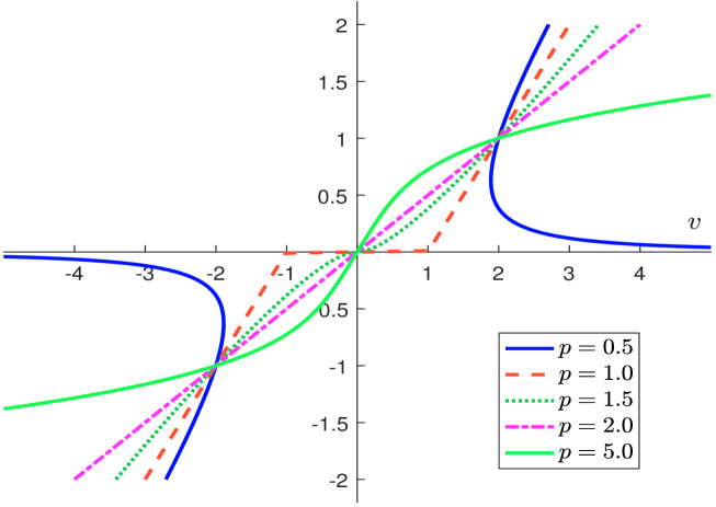
Figure 13: Proximal operator of $\dfrac{1}{p}\left\|x\right\|_{p}^{p}$

A.8.3 The case $f\left(x\right)=\mathds{1}_{\Omega}\left(x\right)$

If we assume that $f\left(x\right)=\mathds{1}_{\Omega}\left(x\right)$ where $\Omega$ is a (convex) set, we have:

$$\mathbf{prox}_{f}\left(v\right) = \arg\min\nolimits_{x}\left\{\mathds{1}_{\Omega}\left(x\right)+\frac{1}{2}\left\|x-v\right\|_{2}^{2}\right\}$$

$$= \mathcal{P}_{\Omega}\left(v\right)$$

where $\mathcal{P}_{\Omega}\left(v\right)$ is the standard projection. We give here the results for some polyhedra that are used in portfolio optimization:

$$\Omega$$

If $f$ is a norm, then $f^{\ast}\left(x\right)=\mathds{1}_{\mathcal{B}}\left(x\right)$ where $\mathcal{B}$ is the unit ball of the dual norm of $f$. Thus, Moreau decomposition yields:

$$\mathbf{prox}_{\lambda f}\left(v\right)=v-\lambda\mathcal{P}_{\mathcal{B}}\left(\frac{1}{\lambda}v\right)$$

meaning that we only use projections onto norm balls.

A ball for the $L_{\infty}$ norm is a particular case of box constraint. The orthogonal projection onto the unit ball for the $L_{2}$ norm is:

$$\mathcal{P}_{\mathcal{B}}\left(v\right)=\left\{\begin{array}[]{ll}\dfrac{v}{\left\|v\right\|_{2}}&\text{for }\left\|v\right\|_{2}>1\\ v&\text{for }\left\|v\right\|_{2}\leqslant 1\end{array}\right.$$

The projection on the unit ball for the $L_{1}$ norm is less straightforward. It is given by:

$$\mathcal{P}_{\mathcal{B}}\left(v\right)=\mathrm{sign}\left(v\right)\odot\left(\left|v\right|-\lambda\mathbf{1}\right)$$

where $\lambda$ satisfies:

$$\left\|\left|v\right|-\lambda\mathbf{1}\right\|_{1}=1$$ (63)

Equation (63) can be solved by the bi-section algorithm or projected subgradient methods (Duchi et al., 2008).

Remark 8

Note also that the projection onto an $L_{1}$ ball and a simplex are equivalent problems, applying twice the symmetry $x\mapsto-x$.

Projections onto intersections of convex sets are examples in which the computation of the proximal operator reduces to determining a zero of a real-valued function. For instance, the projection onto the intersection of two balls $\mathcal{B}_{p}\cap\mathcal{B}_{q}$ is a particular case of projection onto a sublevel set that is defined by $\left\{x:f\left(x\right)\leqslant R\right\}$ where $f\left(x\right)=\left\|x\right\|_{q}+\mathds{1}_{\mathcal{B}_{p}}\left(x\right)$. Indeed, we consider a non-empty $L_{p}$ ball $\mathcal{B}_{p}$ and a non-empty $L_{q}$ ball $\mathcal{B}_{q}$. The orthogonal projection $\mathcal{P}_{\Omega}$ onto the intersection $\Omega=\mathcal{B}_{p}\cap\mathcal{B}_{q}$ is given by:

$$\mathcal{P}_{\Omega}\left(v\right)=\left\{\begin{array}[]{ll}\mathcal{P}_{\mathcal{B}_{p}}\left(v\right)&\text{if }\mathcal{P}_{\mathcal{B}_{p}}\left(v\right)\in\mathcal{B}_{q}\\ \mathbf{prox}_{f}\left(v\right)&\text{if }\mathcal{P}_{\mathcal{B}_{p}}\left(v\right)\notin\mathcal{B}_{q}\end{array}\right.$$

where $f\left(x\right)=\lambda^{\star}\left\|x\right\|_{p}$ and $\lambda^{\star}$ is a scalar such that $\mathbf{prox}_{f}\left(v\right)\in\partial\mathcal{B}_{q}$ where $\partial\mathcal{B}_{q}$ is the boundary of $\mathcal{B}_{q}$.

We now consider the projection of $v$ on the intersection of a convex set $\Omega$ and a hyperplane $\mathcal{H=}\left\{x\in\mathbb{R}^{n},a\in\mathbb{R}^{n}\setminus\left\{\mathbf{0}\right\}\mid a^{\top}x=b\right\}$. We have:

$$x^{\star} = \mathcal{P}_{\mathcal{H}\cap\Omega}\left(v\right)$$

$$= \arg\min_{x\in\mathcal{H}\cap\Omega}\frac{1}{2}\left\|x-v\right\|_{2}^{2}$$

Leaving the constraint $x\in\Omega$ implicit, we can write the partial Lagrange function for this problem:

$$\mathcal{L}\left(x,\lambda\right) = \frac{1}{2}\left\|x-v\right\|_{2}^{2}+\lambda\left(a^{\top}x-b\right)$$ (64)

$$= \frac{1}{2}\left\|x-\left(v-\lambda a\right)\right\|_{2}^{2}+\lambda\left(a^{\top}v-b\right)-\frac{1}{2}\lambda^{2}\left\|a\right\|_{2}^{2}$$

As strong duality holds, $x^{\star}$ is the optimal solution if, and only if, there exists a scalar $\lambda^{\star}\in\mathbb{R}$ satisfying:

$$x^{\star}\in\arg\min_{x\in\Omega}\mathcal{L}\left(x,\lambda^{\star}\right)\qquad\text{and}\qquad x^{\star}\in\mathcal{H}$$

Using Equation (64), we obtain:

$$x^{\star}=\mathcal{P}_{\Omega}\left(v-\lambda^{\star}a\right)\qquad\text{and}\qquad x^{\star}\in\mathcal{H}$$

where $\lambda^{\star}$ is the solution to the equation:

$$a^{\top}\mathcal{P}_{\Omega}\left(v-\lambda^{\star}a\right)=b$$

Particular cases of the last formula are projections onto the standard simplex $\Omega=\mathbb{R}_{+}^{n}$, the intersection of two non-empty balls $\Omega=\mathcal{B}_{p}\cap\mathcal{B}_{q}$ and the hyperplane $\Omega=\left\{x\in\mathbb{R}^{n}\mid\mathbf{1}^{\top}x=0\right\}$.

A.9 Derivation of the PRESS statistic for the Tikhonov regularization

We have:

$$X^{\top}X=X_{-t}^{\top}X_{-t}+x_{t}x_{t}^{\top}$$

and:

$$X^{\top}Y=X_{-t}^{\top}Y_{-t}+x_{t}y_{t}$$

The Sherman-Morrison-Woodbury formula leads to:

$$\hat{\beta}_{-t} = \left(X_{-t}^{\top}X_{-t}+\varrho_{2}\Gamma_{2}\Gamma_{2}^{\top}\right)^{-1}X_{-t}^{\top}Y_{-t}$$

$$= \left(X^{\top}X+\varrho_{2}\Gamma_{2}\Gamma_{2}^{\top}-x_{t}x_{t}^{\top}\right)^{-1}\left(X^{\top}Y-x_{t}y_{t}\right)$$

$$= \left(S\left(\varrho_{2}\right)^{-1}-x_{t}x_{t}^{\top}\right)^{-1}\left(X^{\top}Y-x_{t}y_{t}\right)$$

$$= \left(S\left(\varrho_{2}\right)+\frac{S\left(\varrho_{2}\right)x_{t}x_{t}^{\top}S\left(\varrho_{2}\right)}{1-x_{t}^{\top}S\left(\varrho_{2}\right)x_{t}}\right)\left(X^{\top}Y-x_{t}y_{t}\right)$$

$$= S\left(\varrho_{2}\right)X^{\top}Y-S\left(\varrho_{2}\right)x_{t}y_{t}+$$

$$\frac{S\left(\varrho_{2}\right)x_{t}x_{t}^{\top}S\left(\varrho_{2}\right)}{1-x_{t}^{\top}S\left(\varrho_{2}\right)x_{t}}X^{\top}Y-\frac{S\left(\varrho_{2}\right)x_{t}x_{t}^{\top}S\left(\varrho_{2}\right)}{1-x_{t}^{\top}S\left(\varrho_{2}\right)x_{t}}x_{t}y_{t}$$

We denote $z_{t}=x_{t}^{\top}S\left(\varrho_{2}\right)x_{t}$. Since $\hat{\beta}=S\left(\varrho_{2}\right)X^{\top}Y$, we get:

$$x_{t}^{\top}\hat{\beta}_{-t}=x_{t}^{\top}\hat{\beta}-z_{t}y_{t}+\frac{z_{t}}{1-z_{t}}x_{t}^{\top}\hat{\beta}-\frac{z_{t}^{2}}{1-z_{t}}y_{t}$$

Finally, we obtain:

$$y_{t}-x_{t}^{\top}\hat{\beta}_{-t} = y_{t}\left(1+z_{t}+\frac{z_{t}^{2}}{1-z_{t}}\right)-x_{t}^{\top}\hat{\beta}\left(1+\frac{z_{t}}{1-z_{t}}\right)$$

$$= y_{t}\left(\frac{1}{1-z_{t}}\right)-x_{t}^{\top}\hat{\beta}\left(\frac{1}{1-z_{t}}\right)$$

$$= \frac{1}{1-x_{t}^{\top}S\left(\varrho_{2}\right)x_{t}}(y_{t}-x_{t}^{\top}\hat{\beta})$$

It follows that the PRESS statistic is equal to:

$$\mathcal{P}\mathrm{ress}\left(\varrho_{2}\right) = \sum_{t=1}^{T}\left(y_{t}-x_{t}^{\top}\hat{\beta}_{-t}\right)^{2}$$

$$= \sum_{t=1}^{T}\frac{\left(y_{t}-x_{t}^{\top}\hat{\beta}\right)^{2}}{\left(1-x_{t}^{\top}S\left(\varrho_{2}\right)x_{t}\right)^{2}}$$

Appendix B The Black-Litterman model

B.1 Computing the implied risk premia

Let us consider the following optimization problem:

$$x^{\star}\left(\gamma\right) = \arg\min\frac{1}{2}x^{\top}\Sigma x-\gamma x^{\top}\left(\mu-r\mathbf{1}\right)$$

s.t. $$\mathbf{1}^{\top}x=1$$

The unscaled solution is:

$$x^{\star}=\gamma\Sigma^{-1}\left(\mu-r\mathbf{1}\right)$$

Given an initial allocation $x_{0}$, we deduce that this portfolio is optimal if the vector of expected returns is defined by:

$$\tilde{\mu}=r+\frac{1}{\gamma}\Sigma x_{0}$$

By assuming that we know the Sharpe ratio of the initial allocation, we deduce that:

$$\tilde{\mu}=r+\mathop{\rm SR}\left(x_{0}\mid r\right)\frac{\Sigma x_{0}}{\sqrt{x_{0}^{\top}\Sigma x_{0}}}$$ (65)

We retrieve one of the fundamental results from the capital asset pricing model. At the optimum, risk premia are proportional to marginal risks (Roncalli, 2013).

B.2 Conditional distribution of expected returns

Black and Litterman (1992) state that vector $R_{t}$ of asset returns follow a Gaussian distribution:

$$R_{t}\sim\mathcal{N}\left(\tilde{\mu},\Sigma_{m}\right)$$

where $\tilde{\mu}$ is the implied expected return associated with the allocation $x_{0}$ and $\Sigma_{m}$ is the market covariance matrix of asset returns. To specify the portfolio manager’s views, they assume that they are given by this relationship:

$$PR_{t}=Q+\varepsilon$$ (66)

where $P$ is a $\left(k\times n\right)$ matrix, $Q$ is a $\left(k\times 1\right)$ vector and $\varepsilon\sim\mathcal{N}\left(0,\Sigma_{\varepsilon}\right)$ is a Gaussian vector of dimension $k$. The $k$ views of the portfolio manager can be expressed in absolute or relative terms. It follows that the joint distribution of the expected returns $R_{t}$ and the views $\nu_{t}=PR_{t}-\varepsilon$ is given by the following relationship:

$$\left(\begin{array}[]{c}R_{t}\\ \nu_{t}\end{array}\right)\sim\mathcal{N}\left(\left(\begin{array}[]{c}\tilde{\mu}\\ P\tilde{\mu}\end{array}\right),\left(\begin{array}[]{cc}\Sigma_{m}&\Sigma_{m}P^{\top}\\ P\Sigma_{m}&P\Sigma_{m}P^{\top}+\Sigma_{\varepsilon}\end{array}\right)\right)$$

By applying the conditional expectation formula, we obtain:

$$\bar{\mu} = \mathbb{E}\left[R_{t}\mid\nu_{t}=Q\right]$$

$$= \tilde{\mu}+\Sigma_{m}P^{\top}\left(P\Sigma_{m}P^{\top}+\Sigma_{\varepsilon}\right)^{-1}\left(Q-P\tilde{\mu}\right)$$

and:

$$\bar{\Sigma} = \mathbb{E}\left[\left(R_{t}-\bar{\mu}\right)\left(R_{t}-\bar{\mu}\right)^{\top}\mid\nu_{t}=Q\right]$$

$$= \Sigma_{m}-\Sigma_{m}P^{\top}\left(P\Sigma_{m}P^{\top}+\Sigma_{\varepsilon}\right)^{-1}P\Sigma_{m}$$

The vector of conditional expected returns $\bar{\mu}$ has two components:

1. The first component corresponds to the vector of implied expected returns $\tilde{\mu}$.

2. The second component is a correction term which takes into account the disequilibrium $\left(Q-P\tilde{\mu}\right)$ between the manager’s views and the market’s views.

In the same way, the conditional covariance matrix has two components. Indeed, we have:

$$\bar{\Sigma} = \left(I_{n}+\Sigma_{m}P^{\top}\Sigma_{\varepsilon}^{-1}P\right)^{-1}\Sigma_{m}$$ (67)

$$= \left(\Sigma_{m}^{-1}+P^{\top}\Sigma_{\varepsilon}^{-1}P\right)^{-1}$$

Again, the conditional covariance matrix is a weighted average of the market covariance matrix $\Sigma_{m}$ and the covariance matrix $\Sigma_{\varepsilon}$ of the manager views.

B.3 The case of absolute views

If the portfolio manager specifies absolute views, it is equivalent imposing $P=I_{n}$ and $Q=\breve{\mu}$. We deduce that:

$$\bar{\mu}=\left(I_{n}-\Sigma_{m}\left(\Sigma_{m}+\Sigma_{\varepsilon}\right)^{-1}\right)\tilde{\mu}+\Sigma_{m}\left(\Sigma_{m}+\Sigma_{\varepsilon}\right)^{-1}\breve{\mu}$$

and:

$$\bar{\Sigma}=\Sigma_{m}\left(\Sigma_{m}+\Sigma_{\varepsilon}\right)^{-1}\Sigma_{\varepsilon}$$

If we consider the (unscaled) optimal portfolio $\bar{x}$, we obtain:

$$\bar{x} = \gamma\bar{\Sigma}^{-1}\bar{\mu}$$

$$= \gamma\Sigma_{\varepsilon}^{-1}\left(\Sigma_{m}+\Sigma_{\varepsilon}\right)\Sigma_{m}^{-1}\left(\left(I_{n}-\Sigma_{m}\left(\Sigma_{m}+\Sigma_{\varepsilon}\right)^{-1}\right)\tilde{\mu}+\Sigma_{m}\left(\Sigma_{m}+\Sigma_{\varepsilon}\right)^{-1}\breve{\mu}\right)$$

$$= \Sigma_{m}^{-1}\Sigma\tilde{x}+\breve{x}$$

where $\breve{x}$ is the mean-variance optimized portfolio based on the manager’s views. In particular, if $\Sigma_{m}=\Sigma$, it follows that the optimal portfolio $\bar{x}$ is simply the sum of the SAA portfolio $\tilde{x}$ and the MVO portfolio $\breve{x}$.

Let $\hat{\Sigma}$ be the empirical covariance matrix. If we assume that $\Sigma_{m}=\tau\hat{\Sigma}$ and $\Sigma_{\varepsilon}=\tau\hat{\Sigma}$, we obtain:

$$\bar{\mu}=\frac{\tilde{\mu}+\breve{\mu}}{2}$$

and:

$$\bar{\Sigma}=\frac{\tau}{2}\hat{\Sigma}$$

The conditional expected returns are therefore an average between the implied expected returns and the manager’s views, whereas the conditional covariance matrix is proportional to the empirical covariance matrix. In particular, if $\tau$ is set to $1$, asset volatilities are divided by $\sqrt{2}$. This type of parametrization is a real problem, because it dramatically reduces the covariance matrix of asset returns.

We now consider a second approach with $\Sigma_{m}=\hat{\Sigma}$ and $\Sigma_{\varepsilon}=\tau\hat{\Sigma}$. It follows that:

$$\bar{\mu}=\frac{\tau}{1+\tau}\tilde{\mu}+\frac{1}{1+\tau}\breve{\mu}$$ (68)

and:

$$\bar{\Sigma}=\frac{\tau}{1+\tau}\hat{\Sigma}$$

When $\tau\rightarrow 0$, we verify that that the conditional expectation tends toward the manager’s views. However, the covariance matrix also tends towards the null matrix (see Figure 14). Again, we notice an arbitrage between the weight of the manager’s views and the reduction of the covariance matrix.

In practice, we would like to control the contribution of the manager’s views without modifying necessarily the covariance matrix of asset returns. This is why we can impose that $\bar{\Sigma}=\hat{\Sigma}$.

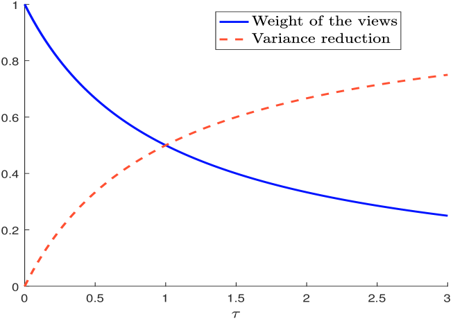
Figure 14: Variance reduction in the Black-Litterman model

Appendix C Additional results

C.1 Tables

Table 19: Quality representation of each asset

Factor		1	2	3	4
Asset	$\quad 1\quad$	$58.35\%$	$0.08\%$	$0.24\%$	$41.33\%$
	$2$	$55.18\%$	$5.90\%$	$38.46\%$	$0.46\%$
	$3$	$50.25\%$	$39.36\%$	$9.07\%$	$1.32\%$
	$4$	$78.91\%$	$18.87\%$	$0.99\%$	$1.23\%$

Table 20: Contribution of each asset

Factor		1	2	3	4
Asset	$\quad 1\quad$	$13.07\%$	$0.06\%$	$0.33\%$	$86.54\%$
	$2$	$17.80\%$	$6.49\%$	$74.32\%$	$1.38\%$
	$3$	$20.02\%$	$53.43\%$	$21.64\%$	$4.91\%$
	$4$	$49.11\%$	$40.02\%$	$3.71\%$	$7.16\%$

Table 21: Linear dependence between the four assets ($\mu_{1}=3\%$)

Asset	$\alpha_{i}$	$\beta_{i}$				$\mathfrak{R}^{2}_{i}$
1	$-2.30\%$		$0.139$	$0.187$	$0.250$	$45.83\%$
2	${\hskip 8.0pt}2.98\%$	$0.230$		$0.268$	$0.191$	$37.77\%$
3	${\hskip 8.0pt}4.49\%$	$0.409$	$0.354$		$0.045$	$33.52\%$
4	${\hskip 8.0pt}4.41\%$	$0.750$	$0.347$	$0.063$		$41.50\%$

Table 22: Risk/return analysis of hedging portfolios ($\mu_{1}=3\%$)

Asset	$\mu_{i}$	$\hat{\mu}_{i}$	$\alpha_{i}$	$\sigma_{i}$	$\hat{\sigma}_{i}$	$s_{i}$	$\mathfrak{R}^{2}_{i}$
1	${\hskip 5.0pt}3.00\%$	$5.30\%$	$-2.30\%$	$15.00\%$	$10.16\%$	$11.04\%$	$45.83\%$
2	${\hskip 5.0pt}8.00\%$	$5.02\%$	${\hskip 8.0pt}2.98\%$	$18.00\%$	$11.06\%$	$14.20\%$	$37.77\%$
3	${\hskip 5.0pt}9.00\%$	$4.51\%$	${\hskip 8.0pt}4.49\%$	$20.00\%$	$11.58\%$	$16.31\%$	$33.52\%$
4	$10.00\%$	$5.59\%$	${\hskip 8.0pt}4.41\%$	$25.00\%$	$16.11\%$	$19.12\%$	$41.50\%$

Table 23: Optimal portfolio ($\mu_{1}=3\%$)

Asset	$\omega_{i}$	$y^{\star}_{i}$	$z^{\star}_{i}$	$x^{\star}_{i}$
1	$84.62\%$	$53.59\%$	$206.52\%$	$-75.81\%$
2	$60.68\%$	$99.25\%$	$164.80\%$	${\hskip 8.0pt}59.46\%$
3	$50.43\%$	$90.44\%$	$135.19\%$	${\hskip 8.0pt}67.87\%$
4	$70.94\%$	$64.31\%$	${\hskip 5.0pt}86.63\%$	${\hskip 8.0pt}48.48\%$

C.2 Figures

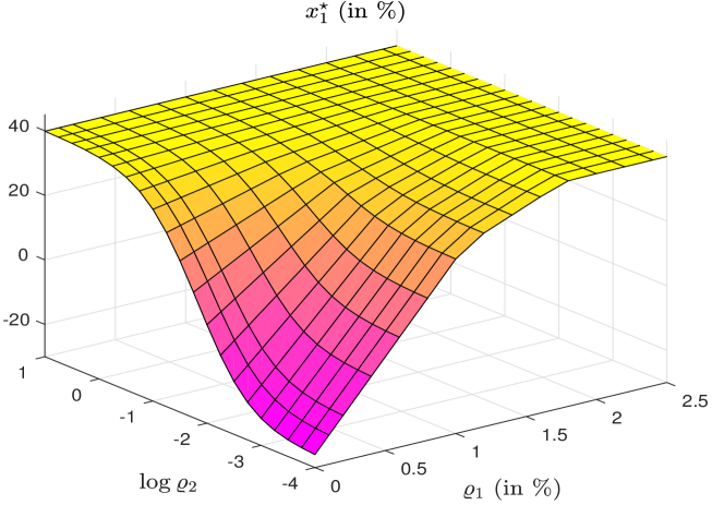
Figure 15: Mixed regularization with a target portfolio ($x_{1}^{\star}$)

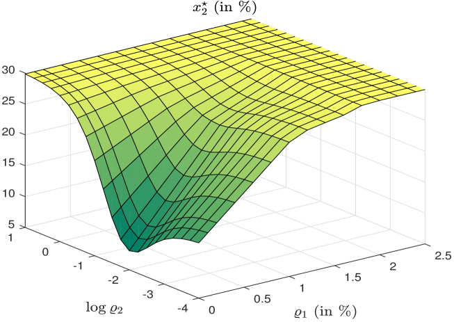
Figure 16: Mixed regularization with a target portfolio ($x_{2}^{\star}$)

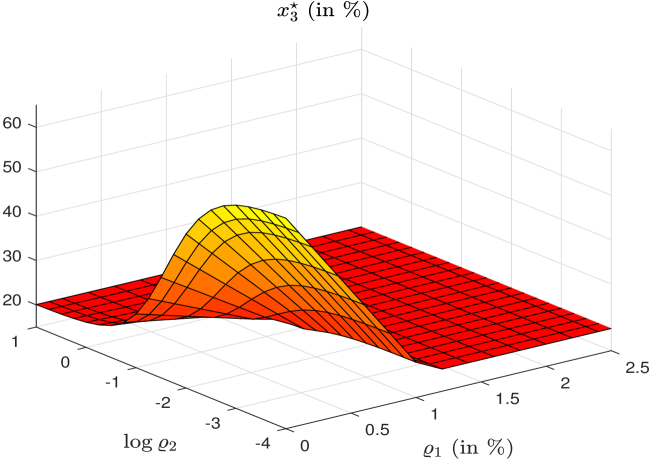
Figure 17: Mixed regularization with a target portfolio ($x_{3}^{\star}$)

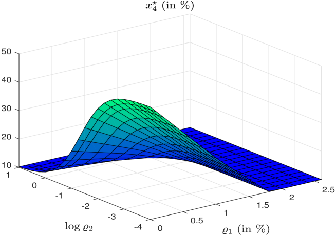
Figure 18: Mixed regularization with a target portfolio ($x_{4}^{\star}$)

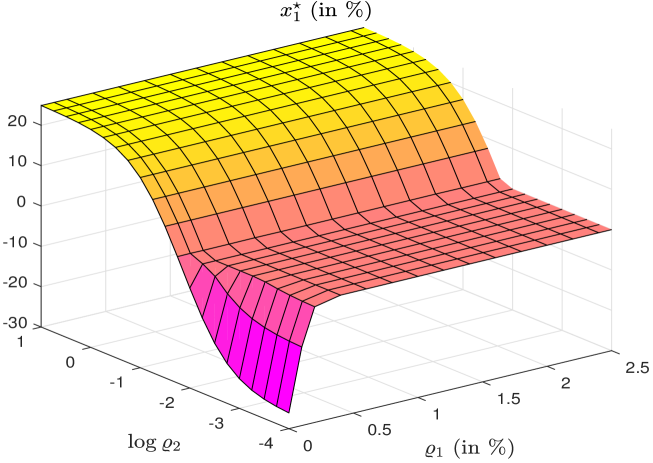
Figure 19: Mixed regularization without a target portfolio ($x_{1}^{\star}$)

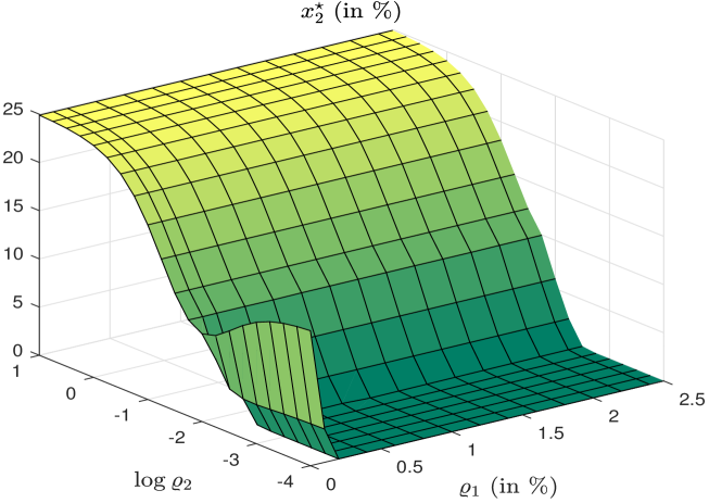
Figure 20: Mixed regularization without a target portfolio ($x_{2}^{\star}$)

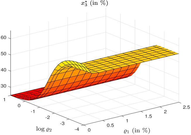
Figure 21: Mixed regularization without a target portfolio ($x_{3}^{\star}$)

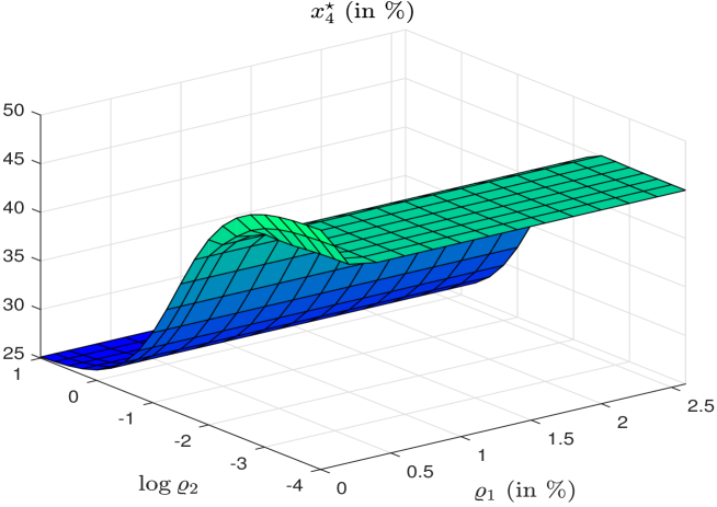
Figure 22: Mixed regularization without a target portfolio ($x_{4}^{\star}$)

References

- [1] Allen, D.M. (1971), Mean Square Error of Prediction as a Criterion for Selecting Variables, Technometrics, 13(3), pp. 469-475.
- [2] Allen, D.M. (1974), The Relationship Between Variable Selection and Data Augmentation and a Method For Prediction, Technometrics, 16(1), pp. 125-127.
- [3] Beck, A. (2017), First-Order Methods in Optimization, MOS-SIAM Series on Optimization, 25, SIAM.
- [4] Black, F. and Litterman, R.B. (1991), Asset Allocation: Combining Investor Views with Market Equilibrium, Journal of Fixed Income, 1(2), pp. 7-18.
- [5] Black, F. and Litterman, R.B. (1992), Global Portfolio Optimization, Financial Analysts Journal, 48(5), pp. 28-43.
- [6] Boyd, S., Parikh, N., Chu, E., Peleato, B., and Eckstein, J. (2010), Distributed Optimization and Statistical Learning via the Alternating Direction Method of Multipliers, Foundations and Trends® in Machine learning, 3(1), pp. 1-122.
- [7] Broadie, M. (1993), Computing Efficient Frontiers using Estimated Parameters, Annals of Operations Research, 45(1), pp. 21-58.
- [8] Brodie, J., Daubechies, I., De Mol, C., Giannone, D., and Loris, I. (2009), Sparse and Stable Markowitz Portfolios, Proceedings of the National Academy of Sciences, 106(30), pp. 12267-12272.
- [9] Bruder, B., Gaussel, N., Richard, J-C., and Roncalli, T. (2013), Regularization of Portfolio Allocation, SSRN, www.ssrn.com/abstract=2767358.
- [10] Candelon, B., Hurlin, C., and Tokpavi, S. (2012), Sampling Error and Double Shrinkage Estimation of Minimum Variance Portfolios, Journal of Empirical Finance, 19(4), pp. 511-527.
- [11] Combettes, P.L., and Müller, C.L. (2018), Perspective Functions: Proximal Calculus and Applications in High-dimensional Statistics, Journal of Mathematical Analysis and Applications, 457(2), pp. 1283-1306.
- [12] Craven, P., and Wahba, G. (1978), Smoothing Noisy Data with Spline Functions, Numerische Mathematik, 31(4), pp. 377-403.
- [13] Diamond, S., Takapoui, R., and Boyd, S. (2018), A General System for Heuristic Solution of Convex Problems over Nonconvex Sets, Optimization Methods and Software, 33(1), pp. 165-193.
- [14] DeMiguel, V., Garlappi, L., Nogales, F.J., and Uppal, R. (2009), A Generalized Approach to Portfolio Optimization: Improving Performance by Constraining Portfolio Norms, Management Science, 55(5), pp. 798-812.
- [15] DeMiguel, V., Garlappi, L., and Uppal, R. (2009), Optimal Versus Naive Diversification: How Inefficient is the 1/N Portfolio Strategy?, Review of Financial Studies, 22(5), pp. 1915-1953.
- [16] DeMiguel, V., Martin-Utrera, A., and Nogales, F.J. (2013), Size Matters: Optimal Calibration of Shrinkage Estimators for Portfolio Selection, Journal of Banking & Finance, 37(8), pp. 3018-3034.
- [17] Duchi, J., Shalev-Shwartz, S., Singer, Y., and Chandra, T. (2008), Efficient Projections onto the -ball for Learning in High Dimensions, in Cohen, W. (Ed.), ICML ’08: Proceedings of the 25th International Conference on Machine Learning, ACM, pp. 272-279.
- [18] Engl, H.W., Hanke, M., and Neubauer, A. (1996), Regularization of Inverse Problems, Mathematics and Its Applications, 375, Springer.
- [19] Fisch, J.E., Laboure, M., and Turner, (2017), The Economics of Complex Decision Making: The Emergence of the Robo Adviser, Working paper.
- [20] Gabay, D. (1983), Applications of the Method of Multipliers to Variational Inequalities, in Fortin, M., and Glowinski, R. (Eds), Augmented Lagrangian Methods: Applications to the Numerical Solution of Boundary-Value Problems, Studies in Mathematics and Its Applications, 15, pp. 299-331, Elsevier.
- [21] Gabay, D., and Mercier, B. (1976), A Dual Algorithm for the Solution of Nonlinear Variational Problems via Finite Element Approximation, Computers & Mathematics with Applications, 2(1), pp. 17-40.
- [22] Gârleanu, N., and Pedersen, L.H. (2013). Dynamic Trading with Predictable Returns and Transaction Costs, Journal of Finance, 68(6), pp. 2309-2340.
- [23] Ghadimi, E., Teixeira, A., Shames, I., and Johansson, M. (2015), Optimal Parameter Selection for the Alternating Direction Method of Multipliers (ADMM): Quadratic Problems, IEEE Transactions on Automatic Control, 60(3), pp. 644-658.
- [24] Giselsson, P., and Boyd, S. (2017), Linear Convergence and Metric Selection for Douglas-Rachford Splitting and ADMM, IEEE Transactions on Automatic Control, 62(2), pp. 532-544.
- [25] Golub, G.H., Heath, M., and Wahba, G. (1979), Generalized Cross-validation as a Method for Choosing a Good Ridge Parameter, Technometrics, 21(2), pp. 215-223.
- [26] Grinold, R.C. (1994), Alpha is Volatility Times IC Times Score, or Real Alphas Don’t Get Eaten, Journal of Portfolio management, 20(4), pp. 9-16.
- [27] Hadamard, J. (1902), Sur les Problèmes aux Dérivées Partielles et Leur Signification Physique, Princeton University Bulletin, 13, pp. 49-52.
- [28] Hallerbach, W.G. (2012), A Proof of the Optimality of Volatility Weighting over Time, Journal of Investment Strategies, 1(4), pp. 87-99.
- [29] Hastie, T., Tibshirani, R. and Friedman, J. (2009), The Elements of Statistical Learning, Second edition, Springer.
- [30] He, B.S., Yang, H., and Wang, S.L. (2000), Alternating Direction Method with Self-Adaptive Penalty Parameters for Monotone Variational Inequalities, Journal of Optimization Theory and applications, 106(2), pp. 337-356.
- [31] Hocquard, A., Ng, S., and Papageorgiou, N. (2013), A Constant-volatility Framework for Managing Tail Risk, Journal of Portfolio Management, 39(2), pp. 28-40.
- [32] Hoerl, A.E. and Kennard, R.W. (1970), Ridge Regression: Biased Estimation for Nonorthogonal Problems, Technometrics, 12(1), pp. 55-67.
- [33] Hutchinson, M.F., and De Hoog, F.R. (1985), Smoothing Noisy Data with Spline functions, Numerische Mathematik, 47(1), pp. 99-106.
- [34] Jagannathan, R., and Ma, T. (2003), Risk Reduction in Large Portfolios: Why Imposing the Wrong Constraints Helps, Journal of Finance, 58(4), pp. 1651-1684.
- [35] Jorion, P. (1988), Bayes-Stein Estimation for Portfolio Analysis, Journal of Financial and Quantitative Analysis, 21(3), pp. 279-292.
- [36] Jorion, P. (1992), Portfolio Optimization in Practice, Financial Analysts Journal, 48(1), pp. 68-74.
- [37] Laloux, L., Cizeau, P., Bouchaud, J-P., and Potters, M. (1999), Noise Dressing of Financial Correlation Matrices, Physical Review Letters, 83(7), pp. 1467-1470.
- [38] Ledoit, O., and Wolf M. (2003), Improved Estimation of the Covariance Matrix of Stock Returns With an Application to Portfolio Selection, Journal of Empirical Finance, 10(5), pp. 603-621.
- [39] Ledoit O. and Wolf M. (2004), Honey, I Shrunk the Sample Covariance Matrix, Journal of Portfolio Management, 30(4), pp. 110-119.
- [40] Malongo, H., Lezmi, E., Phung-Que, B., and Roncalli, T., (2016), Asset Allocation for Robo-Advisors, Amundi Internal Research Paper.
- [41] Maillard, S., Roncalli, T., and Teïletche, J. (2010), The Properties of Equally Weighted Risk Contribution Portfolios, Journal of Portfolio Management, 36(4), pp. 60-70.
- [42] Markowitz, H. (1952), Portfolio Selection, Journal of Finance, 7(1), pp. 77-91.
- [43] Markowitz, H. (1956), The Optimization of a Quadratic Function Subject to Linear Constraints, Naval Research Logistics Quarterly, 3(1-2), pp. 111-133.
- [44] Martellini, L. (2016), Mass Customization Versus Mass Production – How an Industrial Revolution is About to Take Place in Money Management and Why It Involves a Shift from Investment Products to Investment Solutions, Journal of Investment Management, 14(3), pp. 5-13.
- [45] Michaud, R.O. (1989), The Markowitz Optimization Enigma: Is ‘Optimized’ Optimal?, Financial Analysts Journal, 45(1), pp. 31-42.
- [46] Parikh, N., and Boyd, S. (2014), Proximal Algorithms, Foundations and Trends® in Optimization, 1(3), pp. 127-239.
- [47] OECD (2017), Robo-Advice for Pensions, OECD Report, http://www.oecd.org/going-digital.
- [48] Raghunathan, A.U., and Di Cairano, S. (2014). ADMM for Convex Quadratic Programs: Q-linear Convergence and Infeasibility Detection, arXiv, 1411.7288.
- [49] Richard, J-C., and Roncalli, T. (2015), Smart Beta: Managing Diversification of Minimum Variance Portfolios, in Jurczenko, E. (Ed.), Risk-based and Factor Investing,, ISTE Press – Elsevier.
- [50] Roncalli, T. (2013), Introduction to Risk Parity and Budgeting, Chapman & Hall/CRC Financial Mathematics Series.
- [51] Roncalli, T. (2015), Introducing Expected Returns into Risk Parity Portfolios: A New Framework for Asset Allocation, Bankers, Markets & Investors, 138, pp. 18-28.
- [52] Roncalli, T. (2017), Alternative Risk Premia: What Do We Know?, in Jurczenko, E. (Ed.), Factor Investing and Alternative Risk Premia, ISTE Press – Elsevier.
- [53] Scherer, B. (2007), Portfolio Construction & Risk Budgeting, Third edition, Risk Books.
- [54] Sharpe, W.F. (1963), A Simplified Model for Portfolio Analysis, Management Science, 9(2), pp. 277-293.
- [55] Sharpe, W.F. (1964), Capital Asset Prices: A Theory of Market Equilibrium under Conditions of Risk, Journal of Finance, 19(3), pp. 425-442.
- [56] Stevens, G.V.G. (1998), On the Inverse of the Covariance Matrix in Portfolio analysis, Journal of Finance, 53(5), pp. 1821-1827.
- [57] Stone, M. (1974), Cross-validation and Multinomial Prediction, Biometrika, 61(3), pp. 509-515.
- [58] Stone, M. (1977), An Asymptotic Equivalence of Choice of Model by Cross-validation and Akaike’s Criterion, Journal of the Royal Statistical Society B, 39(1), pp. 44-47.
- [59] Stone, M. (1978), Cross-validation: A Review, Statistics: A Journal of Theoretical and Applied Statistics, 9(1), pp. 127-139.
- [60] Tibshirani, R. (1996), Regression Shrinkage and Selection via the Lasso, Journal of the Royal Statistical Society B, 58(1), pp. 267-288.
- [61] Wahba, G. (1977), Practical Approximate Solutions to Linear Operator Equations when the Data are Noisy, SIAM Journal on Numerical Analysis, 14(4), pp. 651-667.
- [62] Wang, S.L., and Liao, L.Z. (2001), Decomposition Method with a Variable Parameter for a Class of Monotone Variational Inequality Problems, Journal of Optimization Theory and Applications, 109(2), pp. 415-429.
- [63] Zou, H., and Hastie, T. (2005), Regularization and Variable Selection via the Elastic Net, Journal of the Royal Statistical Society Series B, 67(2), pp. 301-320.