Photoionization Emission Models for the Cyg X-3 X-ray Spectrum

Abstract

We present model fits to the X-ray line spectrum of the well known High Mass X-ray binary Cyg X-3. The primary observational dataset is a spectrum taken with the $Chandra$ X-ray Observatory High Energy Transmission Grating (HETG) in 2006, though we compare it to all the other observations of this source taken so far by this instrument. We show that the density must be $\geq 10^{12}$ cm^-3 in the region responsible for most of the emission. We discuss the influence of the dust scattering halo on the broad band spectrum and we argue that dust scattering and extinction is not the most likely origin for the narrow feature seen near the Si K edge. We identify the features of a wind in the profiles of the strong resonance lines and we show that the wind is more apparent in the lines from the lighter elements. We argue that this wind is most likely associated with the companion star. We show that the intensities of most lines can be fitted, crudely, by a single component photoionized model. However, the iron K lines do not fit with this model. We show that the iron K line variability as a function of orbital phase is different from the lower energy lines, which indicates that the lines arise in physically distinct regions. We discuss the interpretation of these results in the context of what is known about the system and similar systems.

1. Introduction

Cygnus X-3 (4U 2030+40, V1521 Cyg) is a high-mass X-ray binary (HMXB) which is peculiar owing to its short orbital period (P = 4.8 h; Parsignault et al. 1972) and its radio brightness ( 100 mJy in a quiescent state, up to 20 Jy during outbursts; e.g. Waltman et al. 1995). The most likely distance to the source is 7.4$\pm$1.1 kpc (McCollough et al., 2016, 2013). The companion is a WN4-6 type Wolf-Rayet (WR) star (van Kerkwijk et al., 1992, 1996; Koljonen and Maccarone, 2017). In the X-ray band, many of the observational features of Cyg X-3 are likely due to the strong wind from the companion star (Paerels et al., 2000; Szostek & Zdziarski, 2008; Zdziarski et al., 2010, 2012). The wind absorbs and scatters X-rays from the compact object, and produces the broad sinusoidal orbital light curve (Willingale et al., 1985; Zdziarski et al., 2012). The material responsible for this behavior also prevents unobscured observation of the compact X-ray source (the exception being jet ejection events, where the ram pressure of the jet can displace the stellar wind; (Koljonen et al., 2018). A quantitative understanding of the wind thus can aid in disentangling its effect on the observed properties of Cyg X-3 from the intrinsic properties of the compact object.

Observations in the 1-10 keV band reveal very strong line emission (Serlemitsos et al., 1975); in the hard state, Hjalmarsdotter et al. (2008) found equivalent widths $\sim$0.2 keV, softer states have 0.2-0.4 keV (Koljonen et al., 2010, 2018). The most likely scenario for this emission is reprocessing of continuum X-rays by the wind. If so, these lines provide sensitive constraints on the conditions in the wind and other structures in the binary (Paerels et al., 2000). Study of these lines is aided by the brightness of Cyg X-3, making it relatively well suited to study with current X-ray spectrometers. The spectrum is highly cut off by interstellar attenuation, with an average equivalent hydrogen column density of $\geq 10^{22}$ cm^-2 (Kalberla et al., 2005). The X-ray line spectrum shows emission from ions of all abundant elements visible at energies above 1 keV, from Mg through Fe. These indicate the importance of photoionization as an excitation mechanism in the line emitting gas. Observations using the Chandra High Energy Transmission Grating (HETG) have provided insights including the presence of radiative recombination continua (RRCs) which constrain the the gas temperature (Paerels et al., 2000), orbital modulation of the emission line centroids (Stark & Saia, 2003), and P Cygni profiles which constrain the masses of the two stars (Vilhu et al., 2009).

Spectra of Cyg X-3 obtained by the Chandra HETG are affected by the brightness of the source, leading to pileup when data is taken in the timed-event (TE) mode, and also by the variability of the source over timescales long compared with the binary period. As we show in this paper, there is variability present in the lines also along the orbit. In addition to the studies of temperature and dynamics published so far, the X-ray line spectrum contains information on the density, elemental abundances, and ionization mechanism in the emitting gas. Until now, there has not been an analysis of the entire spectrum obtained by the HETG which addresses these topics. In this paper we present model fits to the Chandra HETG spectrum. We focus primarily on one observation taken during a high state, and taken in continuous clocking mode in order to mitigate the effects of pileup. This spectrum was previous reported by Vilhu et al. (2009). The strong continuum observed from Cyg X-3, together with the detection of RRCs (Liedahl & Paerels, 1996), are indications that the ionization balance and excitation are dominated by photoionization and photoexcitation.

2. Data Analysis

2.1. Chandra Data

The primary datasets used in this analysis were obtained with the Chandra High Energy Transmission Grating (HETG) (Obsids 7268 and 6601, PI McCollough) on 2006 January 25 – 26. The observations started on MJD 53760.59458 (when the source was at X-ray orbital phase 0.053) and went through to MJD 53761.42972 ( X-ray orbital phase 0.240). During these observations Cyg X-3 was in a high soft state (quenched radio state) with an average RXTE/ASM count rate around 30 cps (corresponding to 400 mCrab; typical hard state count rates are less than 10 cps). The observations in Obsid 7268 were done in CC mode (continuous clocking) with a window filter applied to the zeroth order. The observations in Obsid 6601 were done in TE (timed event) mode with a 440 pixel subarray which results in a 1.4 sec frame time. The data were reduced using standard Ciao tools, with appropriate modifications for CC mode data. The average flux during the observation was 9.3 $\times 10^{-9}$ erg cm^-2 s^-1 or approximately 400 mcrab. Although Cyg X-3 is bright enough to permit analysis of the third order spectra, in this paper we work solely with the first order HETG spectra. We will report on analysis of third order spectra in a subsequent paper.

In the case of Obsid 6601 there is a difference between the HEG and MEG with the MEG falling below the HEG spectra in the range of 2.3 to 4.4 Angstrom range (2.8 to 5.4 keV). This is likely evidence of pileup as reported by Corrales & Paerels (2015). They found the pileup was a problem with the MEG spectra (light is dispersed over a smaller angle) but not a major problem with the HEG. Also the the various orders (2 and 3rd) are overlapping in this spectral region. The problem with the MEG spectra is that in addition to reducing (and distorting) the continuum spectra the lines are also impacted even more. As a result of this, in what follows we ignore the MEG data in fitting to Obsid 6601.

In the case of Obsid 7268 we analyze and discuss the spectrum obtained from the +1 and -1 orders of both the HEG and MEG arms of the HETG. These were analyzed simultaneously with the same model applied to both. Analysis was done using the xspec(Arnaud, 1996) analysis program. All fits were performed using the c-statistic (Cash, 1979) and no rebinning was performed during the fitting or the plotting. Plots of the spectrum show just the HEG +1 order spectra for clarity. The CC mode data has the advantage that it will not be affected by pileup. In principle, it can be affected by possible background contamination owing to the effectively much larger spectral extraction region on the ACIS chips. However, in the case of Cyg X-3, the sky background is dominated by the dust scattered halo (Corrales & Paerels, 2015), and the use of CC mode data allows a more accurate treatment of this component than does TE mode. For this reason, in what follows we illustrate many of our results using analysis of the data from Obsid 7268. Fits to Obsid 6601 are included for comparison.

In addition we have analyzed all other available HETG spectra of Cyg X-3, with significant observing time. Exposures and observation dates are given in table 1. Here and in what follows we have experimented with joint fits which allow us to include spectra which contain less than 2 ksec of data. We find that this results in negligible improvements or changes to our fits and so we have not included the short observations in the fits reported here. Obsid 1456_000 was a $\sim$12 ksec observation when Cyg X-3 was transitioning from a flaring state to a quiescent state. Obsid 1456_002 was an $\sim$ 8 ksec exposure obtained two months later and Cyg X-3 was in a quiescent state. Obsid 425 was an observation after a major flare in graded mode. It was done in alternating exposure mode, so there is an e1 (short exposure) and e2 (longer exposure). The longer exposure is $\sim$18.5 ksec long and the short exposure is  0.4 ksec long. Obsid 426 was an observation that was done five days after 425 in graded mode. The longer exposure is  15.7 ksec long and the short exposure is  0.3 ksec long. Obsid 16622 was a calibration observation (done in CC mode) made during a quiescent state. Results from fitting to these spectra are given in subsection 3.9, and in subsection 3.8 since Obsid 16622 was taken in a very low flux state and is discussed separately.

Table 1Cygnus X-3 HETG Chandra Observations

ObsID	Date (MJD)	Instrument	Data Mode	Exp Mode	Exposure (ksec)	Count $\rm Rate^{a}$ (cts/sec)	State
$\rm 101^{b}$	51471	ACIS-S	FAINT	TE	1.95	35.8	t/mf
1456 (obi 0)b	51471	ACIS-S	FAINT	TE	12.12	27.7	t/mf
1456 (obi 2)	51531	ACIS-S	FAINT	TE	8.42	18.0	q/qi
425c	51638	ACIS-S	GRADED	TE	18.54	88.2	fs/mrf
426c	51640	ACIS-S	GRADED	TE	15.68	71.0	fi/mrf
6601	53761	ACIS-S	FAINT	TE	49.56	106.6	h/qu
7268	53761	ACIS-S	CC33-GRADED	CC	69.86	121.4	h/qu
16622d	56833	ACIS-S	CC33-FAINT	CC	28.51	25.9	q/qi

Note. — The states are given as k/s where: k are those of Koljonen et al. (2010) [q: Quiescent, t: Transition, fh: FHXR, fi: FIM, fs: FSXR, and h: Hypersoft] and s are those of Szostek, Zdziarski, & McCollough (2008a) [qi: Quiescent, mf: Minor flaring, su: Suppressed, qu: quenched, mrf: Major flaring, and pf: Post flaring].

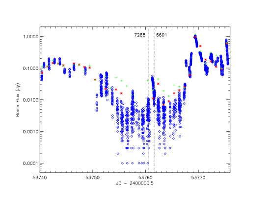
Figure 1.— The 15 GHz (blue diamonds) radio flux densities of Cyg X-3 measured by Ryle telescope (currently the AMI-LA) with the RATAN-600 4.8 GHz (red stars) and 11.2 (green +) daily measurements overlayed. The start times of the Chandra obsids 7268 and 6601 are marked as vertical dotted lines.

Figure 2.— RXTE/ASM lightcurve and hardness ratio showing the long-term soft X-ray (1-10 keV) variability and spectral changes of Cyg X-3 surrounding the Chandra observations 7268 and 6601 (marked as vertical dotted lines).

Figure 3.— Swift/BAT lightcurve showing the long-term hard X-ray (15-50 keV) variability of Cyg X-3 surrounding the Chandra observations 7268 and 6601 (marked as vertical dotted lines).

For the Chandra HETG obsids 7268 and 6601 there was multi-wavelength coverage in the radio, and also from the RXTE and Swift/BAT detectors. Figure 1 shows the Ryle (15 GHz) and RATAN-600 (4.8, 11.2 GHz) observations vs. time. Cyg X-3 is clearly in a quenched radio state. The dotted lines are the start times of the two Chandra grating observations. Figure 2 shows the RXTE ASM count rate and hardness ratio vs. time: This is two day averages of the ASM count rate and the hardness ratio of the 5-12 kev / 3-5 keV bands. This shows Cyg X-3 going into a soft state just prior to the observations. Figure 3 shows the Swift/BAT vs. time. This shows the drop of the hard X-rays (HXR) just prior to the Chandra observations and that Cyg X-3 was in a quenched state. All of these observations show that during the Chandra observations Cyg X-3 was in a quenched/hypersoft state. It is during this state that gamma-ray and major radio flares can occur. During the time of these observations no gamma-ray observations were available and a 1 Jy radio flare occurred several days later (see Fig. 1).

Figure 4 shows the lightcurve taken from the dispersed images during Obsid 7268. This clearly shows features familiar from previous observations: The period is 17253.3 s Vilhu et al. (2009); the minimum flux is not zero, and the lightcurve has a quasi-sinusoidal shape. The eclipse transitions are asymmetric: the egress from eclipse is more gradual than the ingress. The observation spanned almost 4 orbits of the system, and it began just after the minimum. The flux during the minimum is about 30$\%$ of the flux at maximum, similar to the modulation seen by the RXTE ASM (Zdziarski et al., 2012).

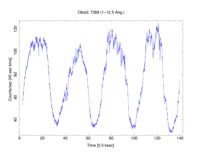
Figure 4.— Lightcurve taken from sum over orders 1 and 3, plus and minus, in the energy band between 1 - 12.5 Å(12.5 – 1 keV) during Obsid 7268. This is the only use of third order data in this paper.

2.2. RXTE Data

We searched for simultaneous pointed RXTE data during the Chandra pointings from the High Energy Astrophysics Science Archive Research Center (HEASARC). This resulted in eight pointings (91090-04-01-00, -04-02-00, -04-03-00, -05-01-00, -05-02-00, -05-03-00, -05-04-00, -05-05-00) with exposures ranging from 3 ksec to 10 ksec. The first pointing started on MJD 53760.4; about 5 hours before the start of the Chandra Obsid 7268, and the last pointing started on MJD 53762.1. We reduced each pointing using HEASOFT 6.22 and standard methods described in the RXTE cookbook. Both the Proportional Counter Array (PCA) and the High Energy X-ray Timing Experiment (HEXTE) data were reduced and spectra were obtained from PCU-2 (all layers) and cluster B, respectively. For spectral analysis, we group the data to a minimum of 5.5 sigma and 2 sigma significance per bin, and ignore bins below 3 keV and above 30 keV, and below 18 keV for PCA and HEXTE, respectively. In addition, 0.5$\%$ and 1$\%$ systematic error were added to all channels for PCA and HEXTE, respectively.

We fit the joint PCA+HEXTE spectra with a simple model including interstellar absorption (phabs), absorption edges from highly-ionized iron (edge or smedge), gaussian from iron K-line (gauss), and blackbody (bbody) convolved with a Comptonization component (simpl). The full model can be described as: phabs*edge(1)*smedge(2)*edge(3)*simpl(bbody+egauss), and it has been successfully used to fit the broad-band X-ray spectra from the hypersoft state previously (Koljonen et al., 2018). Since the PCA is not sensitive to energies where the interstellar attenuation mostly affects the spectrum, we fix the column density to the interstellar value in the direction of Cyg X-3: 1.5 $\times 10^{22}$ cm^-2. The unabsorbed X-ray luminosity (2-100 keV) of the models range from 0.5 — 1.2 $\times 10^{38}$ erg s^-1, the blackbody temperature is constant at 1.2 keV and the Comptonized fraction ranges from 1$\%$ to 5$\%$. Sample spectra are shown in figure 5.

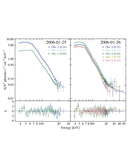
Figure 5.— Spectra taken with RXTE pointed observations. In the figure legend, the X-ray orbital phase is shown in parentheses

2.3. Dust Scattering Halo

A potentially important consideration is the influence of a dust scattering halo on the spectrum. This is because of the relatively large optical extinction toward Cyg X-3, corresponding to $A_{V}\geq$10. This results in a significant optical depth to dust scattering; $\tau_{scatt}\simeq$2 at 1 keV. Dust scattering of X-rays is strongly peaked in the forward direction and will produce what appears to be diffuse emission which is extended on angular scales comparable to or greater than the $Chandra$ ACIS chip size, (Corrales & Paerels, 2015; Ling et al., 2009; Predehl et al., 2000). The total flux in this halo will be comparable to or greater than the source flux below $\simeq$1.5 keV. These effects have been studied in the context of Cyg X-3 by Corrales & Paerels (2015). They showed that the contribution of a dust scattering halo to the flux detected in an annulus from 6 – 100 arcsec away from the central image can be $\geq$ 30$\%$ below 2 keV, decreasing to $\leq$ 10$\%$ above 3 keV.

The ACIS-S chips have a size 8.3 arcminutes perpendicular to the grating dispersion direction. This is sufficient to detect a large fraction of the dust-scattered halo. We have simulated the dust scattered halo from Cyg X-3 using the techniques described in Corrales & Paerels (2015). This shows that a circular region with radius 4.1 arcminutes will include approximately 55$\%$ of the scattered halo at 2 keV, and 98$\%$ of the halo at 7 keV. Images which use CC mode result in the inclusion of all photons hitting the chips as part of the spectrum. Thus, such images will necessarily include the scattering halo as part of the signal spectrum. As a result, the net effect of dust scattering on the spectrum will be greatly reduced; the photons removed from the direct beam by dust scattering will be emitted in the halo, and both will be included in the total spectrum when CC mode is used. Images taken in TE mode use a smaller extraction region, and so will include a smaller fraction of the dust-scattered photons. The energy scale of the HETG in CC mode is based on the position of the detected photons in the direction parallel to the dispersion direction. Thus, all photons which scatter from dust and are reemitted at the same position along the dispersion as they were absorbed will be correctly assigned energies. Dust scattering will have little effect on the flux or energies of these photons (though see the discussion later in this section regarding the Si K edge). Photons which scatter from dust and are reemitted at positions along the dispersion which differ from where they were absorbed will be assigned energies which are incorrect; some will be eliminated by the ACIS energy cuts used for order separation. Nonetheless, approximately half the dust scattered photons will be redistributed by this mechanism into incorrect energies. In what follows we will not attempt to treat this process quantitatively. We emphasize, however, that this affects primarily photons below 1.5 keV, where there are relatively few direct photons, and we do not discuss the analysis of this part of the spectrum in detail.

Photons emitted in the halo will have a longer path to the observatory and so will delayed compared with the direct photons. The delay time is approximately $\sim D\alpha^{2}/2c$, for scatterers located halfway between the source and the observer, where $D$ is the distance and $\alpha$ is the angle of the halo photons relative to the observer’s line of sight, giving delay time $\sim$1 day for $\alpha$=1 arcminute. Thus, with CC mode data, timing information of the scattered light is smeared over several orbital periods. This presents an ultimate limitation on the ability to study time variability from Cyg X-3. But this is most important for photons below $\sim$2 keV; less than 10$\%$ of the photons emitted above 2 keV will be affected by this delay.

In the case of TE mode data, in which the spectrum is accumulated from a region adjacent to the dispersed spectral image, much of the light in the dust scattering halo will fall outside the spectral extraction region. It will therefore not be included in the spectrum to be analyzed and dust scattering will result in a net loss of photons, though again primarily at energies less than $\sim$2 keV. If a background spectrum is extracted from the region of the chip outside the standard source extraction region, and if this is treated as background during analysis of the source spectrum, then there will be an additional loss of flux which ought to be included in the source spectrum. In what follows in our analysis of spectra obtained in TE mode we do not perform any background subtraction. However, our analysis of TE mode data is still affected by the loss of photons due to scattering. Furthermore, dust scattered emission will redistribute photons in the direction parallel to the grating dispersion, and hence likely change their energy assignment. The effects of this process can only be treated in detail with a realistic model for the combined effects of dust scattering and the spectrum extraction. This is beyond the scope of this paper. The effects of this process, combined with the effects of detector pileup, can be crudely evaluated by comparing the spectrum taken in CC mode (obsid 7268) with the spectrum taken at a similar intensity state using TE mode (obsid 6601).

2.4. Orbital Phase Resolved Spectra

We have also extracted the spectral data from both Obsids 7268 and 6601 folded on the X-ray orbital phase. The full observation of Obsid 7268 was 69860 seconds and the total number of counts is 1.06159 $\times 10^{6}$ and so covers approximately 4 binary orbits. We reextract the data and bin into 4 phase bins according to the orbital period of 17252.6 s (Vilhu et al., 2009). We choose phase bins based on the offset from the start of the obsid; this corresponds almost to the minimum in the X-ray light curve, so that we can identify our phases approximately as 0.875-0.125, 0.125-0.375, 0.375-0.625, and 0.625-0.875 We denote these in what follows as phase bins 1,2,3,4. We note that the orbital period of Cyg X-3 is increasing at a rate of $\dot{P}/P\sim 10^{-6}$ yr^-1 (Singh et al., 2002; Bhargava et al., 2017), and that the minimum of the X-ray flux occurs slightly before the phase denoted as superior conjunction, at phase 0.97 (van der Klis & Bonnet-Bidaud, 1989) due to asymmetry of the light curve.

Spectra in each of the phase bins, and the total spectrum for Obsid 7268 (designated T) and the total spectrum for Obsid 16622 (discussed below in subsection 3.8) are displayed in figures 6 – 11. In what follows we first discuss the phase averaged spectrum, and our model fits, and then discuss the variation with orbital phase.

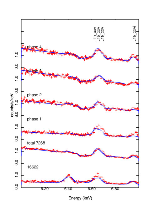
Figure 6.— Spectrum observed by the HETG plotted vs. energy in keV in the 6 – 7 kev energy band. Model shown in blue is described in the text.

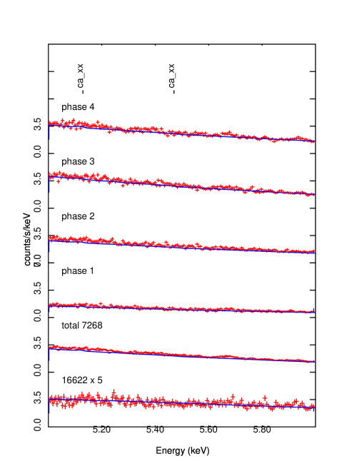
Figure 7.— Spectrum observed by the HETG plotted vs. energy in keV in the 5 – 6 kev energy band.

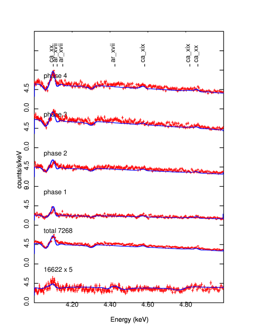
Figure 8.— Spectrum observed by the HETG plotted vs. energy in keV. in the 4 – 5 kev energy band.

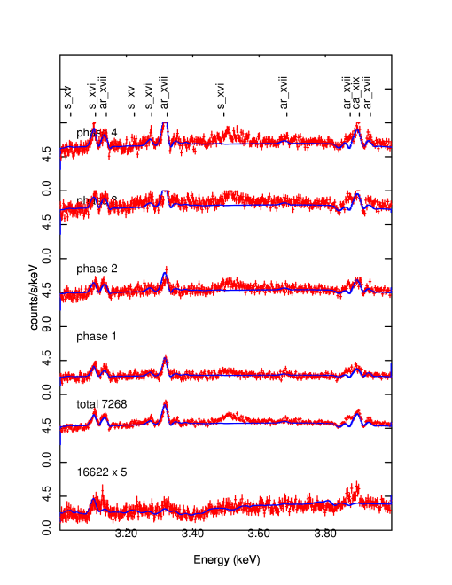
Figure 9.— Spectrum observed by the HETG plotted vs. energy in keV in the 3 – 4 keV energy band.

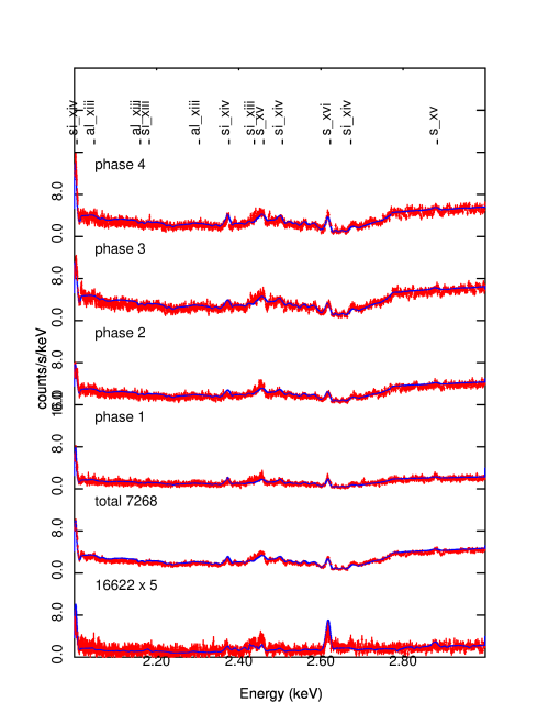
Figure 10.— Spectrum observed by the HETG plotted vs. energy in keV in the 2 – 3 kev energy band.

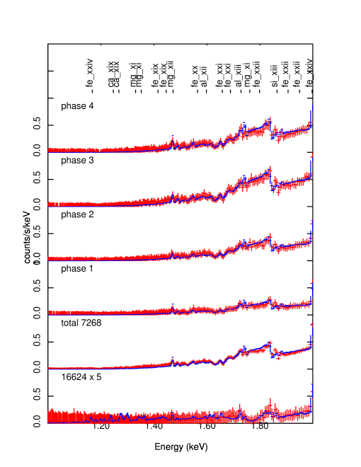
Figure 11.— Spectrum observed by the HETG plotted vs. energy in keV in the 1 – 2 kev energy band. Model is shown in blue and is described in the text. Data has been binned by a factor of 8 for this figure.

3. Results

3.1. Gaussian Fitting

As a first step toward understanding the spectrum, we fit Gaussian profiles for the strongest emission lines and recombination edge model for radiative recombination continua (RRCs) in the total spectrum from Obsid 7268. The list of lines to use as trials for the Gaussians is obtained as follows: we make a model fit to the spectrum using the xstar warmabs/photemis (Kallman & Bautista, 2001) analytic model in xspec. The best fit spectrum yields a list of 194 strongest features. These come from the xstar database, and are level-resolved. We then use the energy/wavelengths of these as trials for Gaussians, and test each one in turn proceeding in order of decreasing energy or increasing wavelength. These lines then also serve as the list of lines from which to derive the line identifications after the fits are performed. RRCs are fitted to a simple exponential shape similar to the ‘redge’ model in xspec. The centroid energies, widths, fluxes, and IDs of the features are listed in table 4 for lines and table 5 for RRCs. The widths of the features, both lines and RRCs, are given in units of km s^-1.

The fitting procedure is designed to allow for the fact that many of the features in the spectrum are broad and represent blends of separate line components. In addition, as we will demonstrate below, there are net offsets in the line peaks or centroids relative to the laboratory wavelength, and these are likely related to Doppler shifts associated with gas motions. Therefore, our procedure is, first, to use the laboratory wavelengths and assume the lines are narrow ($\sigma$=200 km s^-1) in order to test for the presence of a given line. We do this for all the lines in our trial list, and test whether each line improves the fit parameter. Then we allow the centroid, width and flux to vary to find the errors on each quantity. We adopt the $\chi^{2}$ statistic for this automated Gaussian fitting procedure (all other spectral fits in this section use the C-statistic); typical channels in the HETG have $\geq$ 100 counts. We do not allow the line centroid to differ by more than 1000 km s^-1 from the lab (cf. NIST) energy/wavelength, and do not include features for which the best fit width is greater than 10⁴ km s^-1. We consider a feature detected only if it improves the fit by $\Delta\chi^{2}\geq$10 (Avni, 1976). In this way, we try to account for the fact that a given feature may be a blend of separate lines.

Our Gaussian fitting procedure is imperfect, as will be shown below, owing to the fact that the lines are broadened and shifted, and so a given feature in the spectrum may have contributions from various lines. Our level-resolved line list therefore can provide more than one identification for a given spectral feature, using the procedure defined above. And our procedure does not attempt to fit multiple lines to a given feature; if an identification for a feature is found, its region of the spectrum is excluded from further fitting attempts. Thus, there is a bias toward accepting the first plausible identification for a given feature.

Here and in what follows we adopt a simple choice for the continuum in the HETG band: a disk blackbody spectrum as implemented in the diskbb model in xspec (Mitsuda et al., 1984), with a characteristic temperature $kT=1.72$ keV and a normalization which is allowed to vary in order to achieve a good fit. In addition, we find that an additional harder component is needed to fit to the spectrum in the low state. For this we adopt a 2 keV blackbody. We have also experimented with other shapes for these continuum components: for the soft state, a 1.2 keV blackbody plus a power law with index $\gamma$=2.5, (Koljonen et al., 2018) and for the hard state a comptonization model (Hjalmarsdotter et al., 2008; Szostek & Zdziarski, 2008; Hjalmarsdotter et al., 2009; Zdziarski et al., 2010). These models differ from our choice primarily in the flux in the extremes of the energy band away from the peak of the thermal component, i.e. below 2 keV and above $\sim$5 keV. The 1.2 keV blackbody plus power law, compared with the disk blackbody, when fitted to the soft state spectrum Obsid 7268 results in a lower cold column NH and also lower normalization for the emission measure of the high ionization component responsible for the iron K lines. These continuum choices do not result in significantly different values for the goodness of fit criteria C-statistic or $\chi^{2}$, which we attribute to the relatively narrow bandpass of the $Chandra$ HETG plus the predominance of the thermal component within this spectral range. The 2-10 keV flux also is affected by the continuum choice by $\simeq$ 5$\%$. Such different continuum components do correspond to significantly different total fluxes or luminosities for Cyg X-3 when extrapolated to energies outside the HETG bandpass, such as for the RXTE PCA.

RRCs are indicative of radiative recombination. The width of the RRC, as measured by the exponential shape above the threshold, is a measure of the gas temperature (Liedahl & Paerels, 1996). We have fitted the strongest and least blended RRCs, i.e. those from hydrogen-like Si and S, to an analytic ’redge’ model from xspec. This yields, for the Si¹³⁺ RRC at 2.675 keV, a width parameter $T=8.88^{+1.36}_{-2.53}\times 10^{4}$K, and for the S¹⁵⁺ RRC at 3.499 keV the width parameter is $T=3.57^{+3.71}_{-1.77}\times 10^{4}$K. These are both consistent with a temperature $T\simeq 7-8\times 10^{4}$K. This can be compared with the results of photoionization calculations, shown in figure 12, which shows that the model temperature in the region where Si and S are hydrogenic or helium-like is $\geq 10^{5}$K. This suggests additional cooling, such as adiabatic expansion, is affecting the gas in Cyg X-3. The importance of adiabatic expansion cooling depends on the timescale for the gas to flow across a region where the pressure changes significantly when compared with the radiative cooling timescale. As shown by Krolik et al. (1981); Stevens et al. (1992) this can be described by the parameter $\theta=t_{cool}/t_{flow}$; the equilibrium temperature is then reduced by a factor $1/(1+\theta)$. Low temperatures inferred from RRC widths have been observed in other sources: $\gamma^{2}$ Velorum, an WC + O-star binary (Schild et al., 2004), and the planetary nebula BD+30 and its WC9 wind (Nordon et al., 2009). In the latter it was speculated that ions are created by shocks and then cross the contact discontinuity and recombine with unshocked cold electrons. Such a scenario cannot be ruled out for Cyg X-3, though it is notable that the X-ray continuum is adequate to provide the ionization we observe. Comparing the flux in the L$\alpha$ line to the corresponding RRC shows a ratio of $\simeq$13 for Si and $\simeq$11 for S. This can be compared with a predicted ratio $\sim$1 for pure case A recombination (Osterbrock, 1974). Thus it is clear that the L$\alpha$ line emission is affected by other processes. As described below, we consider the most likely such mechanism to be resonance scattering.

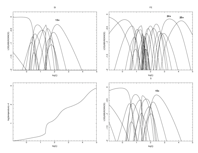
Figure 12.— Ion fractions and temperature for an xstar photoionization equilibrium model using a 1.72 keV diskbb illuminating spectrum. H-like curves are labeled for Si and S, and H- and He-like curves are labeled for Fe. This shows that the temperature in the region where Si and S are hydrogenic or helium-like is $\geq 10^{5}$K.

3.2. He-like Lines

Among the strongest lines in the spectrum are those from the He-like ions. These lines are familiar from the study of other sources and can be crudely described as three components: the resonance ($r$), intercombination ($i$) and forbidden ($f$) lines. The He-like lines are detected in the Chandra HETG spectrum of Cyg X-3 from the elements Mg, Al, Si, S, Ar, Ca and Fe. Table 4 gives values for the difference between the measured line peak and the lab value from NIST in units of km s^-1. These values are constrained to have values in the range -200 km s^-1 to 200 km s^-1 and are given to within 10 km s^-1. Examination of table 4 shows that the energies of the $r$ lines are systematically redshifted relative to the $f$ and $i$ lines by $\sim$200 km s^-1. The Gaussian fits do not clearly detect distinct $r$, $i$, and $f$ components for any of the he-like species. Figure 13 shows the spectrum in the vicinity of the He-like Si lines near 1.8 keV. In this figure, for the purposes of illustration, we force the model lines to be narrow (i.e. width $<$ 10 km s^-1) and at the lab wavelengths for the $r$, $i$ and $f$ components (cf. NIST ). The lab energies for these components are 1.8650, 1.8538 and 1.8395 keV, respectively This clearly shows the three components are present, most notably the $f$ line near 1.84 keV which is not blended with any other component. On the other hand, the feature near 1.86 keV is not centered on the rest wavelength of any tabulated line. It is broad, and therefore spans the region containing the $r$ and $i$ line rest wavelengths. This, together with the deficit of photons at energies near 1.87 keV, above the $r$ line rest energy, is suggestive of a P-Cygni profile. Such profiles were previously identified by Vilhu et al. (2009), and are indicative of outflow in a spherical wind. If so, the 1.86 keV line is formed by resonance scattering of the $r$ line; the absorption corresponds to material seen in projection in front of the continuum source, and the emission corresponds to material seen in reflection. The net blue shift of the absorption and redshift of the emission suggests that the outflow originates at or near the continuum source.

Motivated by this, we fit the lines of Si¹²⁺ with a two component model. One component consists of narrow Gaussians at the rest energies of the $r$, $i$ and $f$ line components. The intercombination line is further separated into three lines corresponding to the three fine structure levels of the 1s2p(³P) term. Here and in what follows we refer to this as the nebular component. We employ a recombination model for this component, the xstar photemis model, which is discussed in section 3.5. The second component is a P-Cygni profile which we model using the Sobolev Exact Integration (SEI) method of Lamers et al. (1987) as implemented in the windabs analytic model in xspec. We employ the photemis and windabs analytic models within xspec, both of which are based on the xstar photoionization models. photemis calculates the emission from a gas in photoionization equilibrium with specified ionization parameter, element abundances, normalization and turbulent velocity. windabs uses the same calculation of ionization balance and temperature, with the important difference that it treats lines excited by photoabsorption from the continuum, and also adds the effects of the gas motion calculated using the Sobolev Exact Integration method (Lamers et al., 1987). It is important to note that photemis is an additive model; that is, it adds to the model spectrum linearly with a given normalization. windabs is a multiplicative model; it imprints features on another model, in our case the continuum. The strength of a multiplicative model is described by a multiplicative factor, in this case the column density of the model wind.

Ion fractions and atomic level populations for both models are calculated using xstar using a specified photoionizing continuum shape, and assuming the gas is optically thin to the ionizing radiation. Details are presented in Kallman & Bautista (2001) and at the xstar webpage . windabs is available as part of the warmabs/photemis package and is described in the xstar manual . The SEI model is described by five parameters: the wind terminal velocity $v_{W}$, the line optical depth parameter $\tau_{line}$, the wind velocity law parameter $\gamma$, the optical depth velocity dependence parameter $\alpha_{1}$ and the line redshift $z$. windabs fixes the values of the last two, $\gamma$=1 and $\alpha_{1}$=1 and calculates $\tau_{line}$ from the specified column density, the elemental abundances and the ion fraction taken from stored xstar results. windabs also allows for departures from spherical symmetry in an ad hoc way by defining a covering fraction, $C$, such that, when 0$\leq C\leq$1, the emission component is reduced by a factor of $C$. When covering fraction $C\geq$1, the absorption component is reduced by a factor $2-C$. At $C=2$, the model produces pure scattered emission. This allows for situations in which the wind is viewed in reflection more than in transmission. It also can crudely simulate situations in which the line thermalization parameter in the wind is not small, though in this case the physical meaning of the covering fraction is lost. The fit to the model consisting of narrow emission, calculated by photemis plus wind emission calculated by windabs, is also shown as the red curve in figure 13. The blue curve in figure 13 shows just the photemis component. This illustrates the fact that, for a recombination-dominated gas, the $r$ line is much weaker than the $f$ or $i$ lines.

P-Cygni profiles were previously identified and fitted by Vilhu et al. (2009). Those authors focused on the lines from the H-like ions, notably Si¹³⁺. We fit the profile of the Si¹²⁺ $r$ line simultaneously with the Si¹³⁺ L$\alpha$ line profile. windabs forces the dynamical quantities ($v_{wind}$, $z$ and $C$) to be the same for the two lines.

Similar results apply to the other He-like lines detected in the Cyg X-3 spectrum. These come from elements S, Ar, Ca and Fe (the lines from Mg and Al are too weak, owing to the low energy cutoff, to permit such a decomposition). That is, all require the presence of both a broad wind line feature in the $r$ line and contributions to the $r$, $i$ and $f$ components which are unshifted and narrow. Figure 15 shows the widths of the wind and narrow components from fits to the various He-like lines. There is a weak indication that the wind component becomes narrower for higher Z elements, i.e. the favored values for wind speed decrease for Ar and Ca, although the errors are large. It also becomes weaker, such that it cannot be detected for Fe. In the case of S the errors on the widths of the higher and lower speed components overlap. The narrow component width is smaller for Ar; the other elements show values for this quantity which are similar to each other.

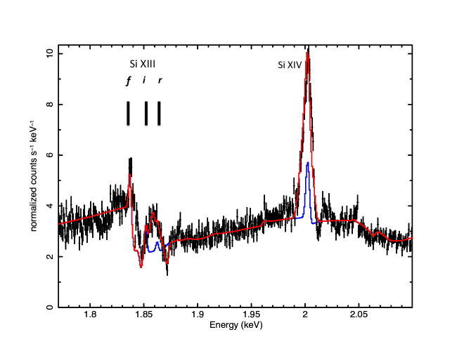
Figure 13.— Spectral region containing the He-like Si lines. The blue curve shows a model consisting of a photoionized emission model, recombination dominated. Positions of the narrow components at the rest wavelengths of the resonance ($r$), intercombination ($i$) and forbidden ($f$) lines are indicated schematically by black lines. The blue and red curves coincide in the region of the $f$ line. This illustrates the fact that the region between the $r$ and $i$ lines is filled in by a redshifted and broadened resonance line component. The red curve shows the total fit including the wind lines.

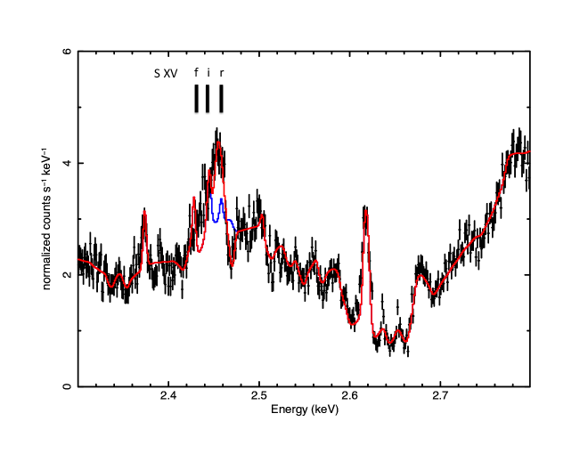
Figure 14.— Spectral region containing the He-like S lines. The blue curve shows a model consisting of a photoionized emission model, recombination dominated. Positions of the narrow components at the rest wavelengths of the resonance ($r$), intercombination ($i$) and forbidden ($f$) lines are indicated schematically by black lines. The blue and red curves coincide in the region of the $f$ line. This illustrates the fact that the region between the $r$ and $i$ lines is filled in by a redshifted and broadened resonance line component. The red curve shows the total fit including the wind lines.

Figure 15.— Widths of the wind and narrow components in km s^-1 vs the nuclear charge of the parent element, i.e. Si=14, S=16, Ar=18, Ca=20, Fe=26. Vertical bars show the allowed regions of width for the wind and nebular components. The upper bar segment corresponding to higher speed and a broader line, eg. for Si, corresponds to the wind, and the lower bar segment with a lower speed and a narrower line corresponds to the nebular model component.

Diagnostic information can be derived from He-like lines when they are described in terms of two ratios: R=$f$/$i$ and G=($f$+$i$)/$r$ (Gabriel & Jordan, 1969). The R ratio depends most sensitively on density, with R $>$ 1 corresponding to density below a critical value which differs according to the element. The G ratio depends on temperature and on the nature of the excitation mechanism. Recombination following photoionization produces G $>>$ 1, while electron impact excitation produces G $<$ 1. In figure 16 we plot values for these ratios allowed by the spectral fits. These ratios utilize values for the $r$ line intensity which are solely from the nebular component of the fit; the wind component and its contribution to the $r$ line are not included.

In a photoionized gas, the properties are conveniently described by the ionization parameter, which is proportional to the ratio of the ionizing flux $F$ to the gas density $n$, log($\xi$)=4$\pi F/n$. Figure 16 also shows the results of a grid of photoionization (xstar) models spanning a range of conditions 1$\leq$log$\xi\leq$3, and 10${}^{5}\leq$T$\leq 10^{6}$K. Colors are as follows: black=silicon, red=sulfur, blue=argon, green=calcium, orange=iron. Model grid values for iron are outside the plotted range. Photoionized gases are typically assumed to have temperature determined by radiative equilibrium between photoionization heating and radiative cooling; here we allow the temperature to vary independently. These models correspond to gas with temperature and ion fractions appropriate to photoionized conditions, and also excitation produced solely by recombination and collisions with thermal electrons. For conditions where the He-like ion is abundant the R ratio is weakly dependent on temperature or ionization parameter, while the G ratio is temperature dependent. This corresponds to the behavior of the grids for Si and S. For Ar and Ca, the range of temperature and ionization parameter spanned by our grid is below the peak of the ion fractional abundance, and the $f$ and $i$ lines are excited primarily by electron impact collisional excitation. As a result the R ratio also depends on the temperature, owing to the temperature dependence of the rate coefficients. The measured values for Fe are also shown by the orange bars in figure 16.

The blending of the $i$ and $f$ lines with each other and with the wind lines results in large error bars in the R and G values for S, Ca, and Fe. In spite of this, there are clear trends to the line ratio values. The fact that R is $\leq$1 for Fe implies a very high density for the formation of this line, i.e. $\geq 10^{17}$ cm^-3. If so, the Fe line formation must occur very close to the continuum source in order to achieve the ionization parameter needed to produce Fe²⁴⁺, i.e. log($\xi)\geq$3. More likely, as we will discuss below, the low energy part of the Fe²⁴⁺ line blend is likely to be affected by absorption, and the true R ratio may be greater than we observe. If all the He-like lines are emitted from the same region, then a trend of the value of R with the atomic number of the parent ion might be expected, since for lower Z ions the density would be closer to the critical density, while for higher Z ions the density could be below the critical density. Figure 16 shows no such trend, possibly due to the large error bars on R for several ions.

The model G ratios are $\geq$4, as expected for recombination at temperatures expected for photoionization. The fact that the measured G ratios are $\sim$2 for Si and Ar is an indication of additional contributions to the $r$ line intensity. A likely explanation is that resonance scattering contributes to the $r$ line intensity even in the nebular component, i.e. the component which does not show dynamical evidence for being in a wind. It is also notable that the measured R ratio is $\leq$1 for most elements. This is in contrast to values $\geq$2 expected for low density recombination for these elements Bautista & Kallman (2000). This is an indication that the density is $\geq 10^{12}$ cm^-3. It is also possible that the R ratio we observe is the result of radiative excitation from the $1s2s(^{3}S)$ upper level of the $f$ line to one of the $1s2p(^{3}P)$ levels. This possibility cannot be evaluated in the absence of any measurement of the flux at the appropriate energy, $\simeq$14.3 eV or $\sim$867 Å . With this caveat, in what follows we will adopt the collisional mechanism. The models used here and in the remainder of this paper adopt a density of $10^{14}$ cm^-3.

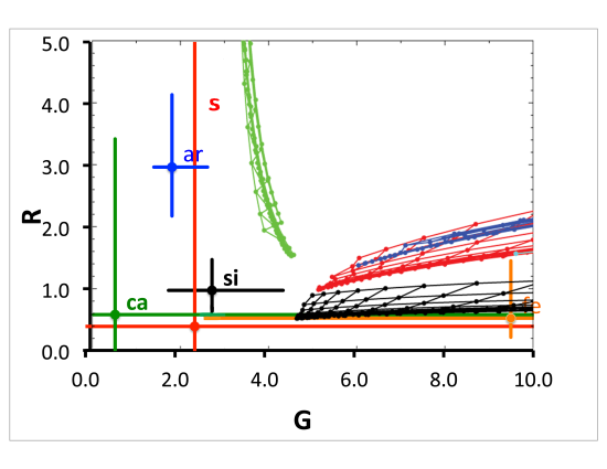
Figure 16.— Values of the two ratios R and G for the narrow components from the various He-like ions. Bars show the values allowed by the spectral fits. The grids show the corresponding regions spanned by photoionization models. Colors are as in figure 15: black=silicon, red=sulfur, blue=argon, green=calcium, orange=iron. Model grid values for iron are outside the plotted range.

3.3. Dust Scattering Scenario for the 1.838 keV Line

The feature at 1.838 keV, which we attribute to the $f$ line of Si¹²⁺ resembles the feature associated with dust scattering from silicate grains. Depending on the grain size, dust scattering can produce a notch-like feature in the total extinction which may appear as an apparent narrow emission feature at energies below the threshold for absorption. This has been illustrated by Corrales et al. (2016) and by Schulz et al. (2016) in $Chandra$ data from GX 3+1, and using laboratory data by Zeegers et al. (2017). This apparent emission feature appears at an energy which is not significantly different than the energy of the feature that we attribute to the Si XIII $f$ line; the lab energy of this line is 1.8398 .

One test of the nebular scenario is whether the nebular component is present in other ions besides Si XIII; if the 1.838 keV feature is due to dust scattering, it should be strongest near the Si K edge and weaker or absent for other elements which are not depleted on dust to the same extent. The depletion of S onto dust is much less than that of Si, approximately 0.4 Draine (2003), so any apparent emission associated with dust scattering on this element would be expected to be much weaker than for Si. The region of the spectrum containing the lines of He-like and H-like S shows emission near the the $f$ line of S XV at 2.43 keV, and also emission near the $i$ lines near 2.44 keV. The lab energies of these lines are 2.430 and 2.448 keV, respectively. However, the shape of the spectrum near these features does not match well with the photemis model. This is illustrated in figure 14.

Further evidence in favor of nebular emission as the origin of the 1.838 keV feature is the fact that the broad feature near 1.845 keV, if it is associated with the P-Cygni emission from the $r$ line, is not likely to be broader than the corresponding feature associated with the Si XIV L$\alpha$ line, near 2 keV. If so, the additional emission from the Si XIII $i$ lines is needed in order to explain the observed width of the 1.845 keV feature. A similar argument applies to the P-Cygni emission from other He-like $r$ lines, notably the S XV line in figure 14.

In addition, the strength of the nebular emission component varies with orbital phase, as shown in section 3.7. This is not expected to occur if the emission near the Si edge were due to dust scattering.

Fits in which the strength of the nebular component is set to zero and a Gaussian is included at 1.84 keV do not provide as good C-statistic values as fits in which the nebular component is included. For example, we find C-statistic/dof=225720/32768 for the Obsid 7268 spectrum summed over orbital phase without the nebular component, as compared with 214748/32768 for the same spectrum fit with the nebular component. In what follows, we will adopt the nebular emission scenario for the line at 1.838 keV but we cannot conclusively rule out the possibility that this line is associated with dust scattering.

3.4. Si K Lines

As shown in the previous subsections, the most abundant ion stage of most elements is the He-like stage. It is of interest to set limits on the strengths of features arising from ions of lower ion stage. This can be done by searching for K lines from ion stages with 3 or more electrons. The existence of these lines and their use as tracers of lower ion stages has been validated using the spectra from other objects, such as Vela X-1 (Sako et al., 2002). Table 2 contains a list of these lines for the obsids 6601 and 7268 spectra.

Table 2Si K Line Fluxes (cm^-2 s^-1)

ion	wavelength (A)	energy (keV)	Obsid_6601	Obsid_7268
V	7.188	1.725	1.98${}^{+0.129}_{-1.80}$	1.48${}^{+0.193}_{-0.180}$
VI	7.125	1.740	0.687${}^{+0.108}_{-0.150}$	0.830${}^{+0.140}_{-0.134}$
VII	7.059	1.756	$\leq$0.002	$\leq$1.389
VIII	6.990	1.774	$\leq$0.013	$\leq$0.187
IX	6.926	1.790	$\leq$0.013	$\leq$0.042
X	6.856	1.808	$\leq$0.009	$\leq$0.012
XI	6.782	1.828	$\leq$0.037	$\leq$0.074
XII	6.906	1.795	$\leq$0.007	$\leq$0.017

This shows that most of these lines are not detected in these spectra. This a manifestation of the fact that the average ionization state of the wind in Cyg X-3 is higher than it is in other HMXBs such as Vela X-1.

3.5. Ionization Balance

In addition to decomposing the line emission into nebular and wind components, it is useful to explore the ionization balance in the line emitting gas. Motivated by the decomposition of the He-like lines into narrow and wind components, we fit the spectrum to a physical model based on realistic ionization balance and emission physics.

The challenge of fitting a single photoionization model to the Cyg X-3 spectrum can be inferred from examination of table 4: the spectrum is dominated by lines from H- and He-like ions of Si, S, Ar, Ca and Fe, and the intensities of the H- and He-like lines from each element are comparable. In contrast, equilibrium ionization balance calculations are affected by the fact that high Z elements have greater rate coefficients for recombination than low Z elements. Therefore high Z elements require a greater ionization rate to achieve a given ionization state. This is compounded by the fact that the ionization cross sections for high Z elements are smaller, so a greater ionizing radiation flux is needed to achieve a given ionization rate. This is true for either thermal electron impact ionization or photoionization. Furthermore, most plausible ionizing spectral energy distributions decrease with energy in the 1-10 keV band. Therefore, the ionization parameter needed to achieve a given ionization state is much greater for high Z elements than it is for low Z elements. The most apparent manifestation of this is the contrast between the lowest Z element with good line detections, Si, compared with the highest Z element, which is Fe. Both the H-like and He-like lines from both elements are detected and have comparable strength ratios. Calculations of photoionized ion balance (Kallman & Bautista, 2001) show that this implies an ionization parameter log($\xi)\simeq$2 for Si, and log($\xi)\geq$4 for Fe. This is illustrated in figure 12. In what follows we refer to this as the ionization balance discrepancy.

A further problem is the fact that gas at log($\xi)\simeq$2 radiates strong iron lines at energies below the energy of the He-like line at 6.7 keV. Such line emission is not consistent with the observed spectrum and can be excluded at a very high level of confidence. This incongruity is difficult to resolve. One possible explanation, which we adopt here, is that there is absorption which removes the iron K emission associated with the log($\xi$)=2 gas. We parameterize this absorption using the ad hoc xspec ’notch’ model component. The notch model is supplied by xspec; it is a multiplicative model with value of unity every where except over a region of specified width around a specified centroid energy, in which the model is reduced by a constant factor $\leq$1. Further evidence for this comes from the weak dip in the spectrum visible near 6.6 keV in the spectra in figure 6. We allow the values of the notch energy, width and depth to vary during fitting. For the total spectrum fit to Obsid 7268 we obtain a value for the energy parameter $\simeq$ 6.56 keV. We fix this value for the phase fits. All our model fits obtain similar values for the other parameters: width $\sim$0.1 keV, and depth $\sim$0.3. Other evidence in favor of this explanation are discussed in the following subsection. The discussion section examines alternative scenarios for the apparent disparity between the conditions needed to explain the iron lines compared with lower energy lines. The high ionization gas responsible for the highly ionized iron emission in this scenario radiates negligible emission from lighter elements and so does not significantly affect the spectrum at lower energies. As discussed below, we also find evidence for a 6.4 keV iron line which we parameterize by a single Gaussian emission model. The contributions of the various components to the iron line are illustrated in figure 17.

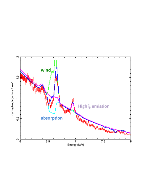
Figure 17.— Iron line region for Obsid 7268 showing components of the model fit: High ionization nebular emission + neutral iron emission (purple), wind emission (green), notch absorption (light blue), total model (dark blue), and observed data (red).

Table 3Model Components

number	name
1	cold absorption
2	notch absorbing iron
3	photoionized nebular emission with log($\xi)\sim$2 - 3
4	6.4 keV Gaussian emission
5	photoionized nebular emission with log($\xi)\sim$4 - 5),
6	wind emission
7	Diskbb
8	Blackbody

The model which we use to fit the global spectrum thus consists of 8 components. These are listed in table 3. In what follows we refer to them by number. This corresponds to the xspec model command ’model wabs*notch(photemis + gaussian + photemis + windabs*(diskbb + bbody))’. We have also experimented with other choices for the neutral absorption, including the ’tbabs’ model. None of the conclusions of this paper are affected by this choice, with the exception of the quantitative value of the absorbing column, which depends on the abundances used; the ’wabs’ model uses fixed abundances. We force the element abundances to be the same for all the model components which depend on them, i.e. components 3,5,6. Parameters of the fits are tabulated in table 6 for the orbital phase summed data and table 7 for the phase resolved data from obsids 6601 and 7268. Also given are the values of the statistical quantities describing the the goodness of fit, the C-statistic and $\chi^{2}$; model fits minimize the value of the C-statistic. Owing to limited statistics, values of parameters for model components 2, 4 and 5, i.e. the notch, Gaussian iron line and high $\xi$ components, contain degeneracies and cannot all be minimized uniquely. Therefore we have frozen the notch width and the $\xi$ value for the high $\xi$ component for most of the spectral fits. Similarly, the element abundances cannot all be uniquely fit for all spectra, so we have used the abundances taken from the spectrum with the best statistics, Obsid 7268, and used them for fitting to most of the other spectra. There are indications of differing abundances, eg. the Fe abundance for Obsid 16622 and the Mg abundance for many of the earlier spectra. The latter may be due to contributions to the low energy part of the spectrum from the dust scattering halo.

The normalizations of the photoionized nebular components are related to the emission measure of the gas and the distance according to the relation $\kappa=\frac{{\rm EM}}{4\pi D^{2}}\times 10^{-10}$. The normalization of component 3, the log($\xi)\simeq$2 - 3 photoionized component, is 429 in the total spectrum for Obsid 7268. The normalization of component 5, the log($\xi)\simeq$4 - 5 photoionized component, is 1035 in this spectrum. These correspond to emission measures of EM=$2.7\times 10^{58}$ cm^-3 and EM=$6.4\times 10^{58}$ cm^-3 for these two components, respectively, assuming a source distance of 7.4 kpc. Abundances in tables 6 and 7 are given in the traditional logarithmic H=12 format; values are generally within 0.5 dex of solar, so we do not clearly identify any strong evidence for processed material. However, we constrain abundances only for elements heavier than Mg, and we cannot constrain the abundance relative to H. We choose Fe to be fixed at a value which produces the total line strength we observe. We have not allowed the value of the turbulent speed to vary during our fitting, due to the degeneracy between the width of the nebular line component and the wind component for many lines. Thus we regard the chosen value, 1600 km s^-1, as an approximate upper limit.

3.6. Iron K Line

As shown in the preceding discussion, the He-like iron K line does not show obvious evidence for a P-Cygni profile. This may be due to the fact that the splitting between the resonance and intercombination lines at iron is less than for lower Z elements, compared with the instrument resolution.

Also notable is the fact that the strong detectable components of the iron line consist of the H-like and He-like features centered at 6.97 and 6.6 keV respectively. The HETG in first order cannot resolve the energy differences of the line centroids of $r$ and $i$, and between $i$ and $f$ components of the He-like iron line, which are 0.033, and 0.031 keV respectively. The width of the He-like feature is 0.015${}^{+0.005}_{-0.0075}$ keV.

The absence of lower ionization features constrains global spectral fits which include self-consistent ionization balance of iron and lower Z elements, as discussed in the previous subsection. Figure 17 shows the spectrum in the vicinity of the iron lines. This reveals a trough centered near 6.55 kev in the total spectrum, and it is possible that this is associated with absorption by intermediate stages of iron. If so, it would account for the existence but non-detection of of lower ionization stages of iron, which must coexist with the He-like Si and S observed at lower energies. A similar feature is observed from the source Circinus X-1 (Schulz et al., 2008).We emphasize that there is no evidence for such an absorbing component elsewhere in the spectrum. As discussed in the previous section, the iron lines do not show evidence for a wind emission component at the same ionization parameter as revealed in the lines from lighter elements, Si, S, Ar, Ca.

The ionization balance of iron relative to lower Z elements depends on the shape of the ionizing radiation spectrum. A power law with photon index $\geq$ 1 has less flux near the ionization thresholds for iron than it does for Si etc., and so produces a greater ionization balance discrepancy than if the ionizing spectrum is flat or inverted in the 1-10 keV band. In fact, a spectrum which increases $\propto\varepsilon^{3}$ is needed to make the iron H/He transition occur at the same ionization parameter as for Si. Such a spectrum is so different from anything we observe that we will not consider it further. An alternative is that the Si – Ca elements are ionized by a spectrum which is soft, such that it does not ionize iron significantly. Experiments show that a kT=1 keV thermal bremsstrahlung spectrum has this property. A thermal bremsstrahlung component has been detected in the Cyg X-3 continuum spectrum (Koljonen et al., 2013) but it has a higher temperature (3-6 keV) than would be needed to account for the Si – Ca ionization observed here. A second component ionized by a much harder spectrum would be needed to account for the H- and He-like iron emission. There is evidence for such a harder component from the RXTE spectra. However, the degree of fine-tuning required for the low energy component and the fact that there is no direct evidence for such a component (i.e. the observed continuum in the Chandra HETG band is more energetic) lead us to consider this scenario to be implausible and we do not consider it further. It is also possible that the region responsible for most of the Fe K emission is closer to the continuum source than the region responsible for the lower Z element emission, and that the Fe K region absorbs the continuum illuminating the lower-Z emission region. We have attempted to simulate this, using xstar, and conclude that fairly fine tuning of the Fe K region is needed in order to preferentially absorb the photons above 6 keV. However, this scenario is difficult to rule out conclusively.

Also apparent in figure 17 is emission near 6.4 keV in the total spectrum for Obsid 7268. This is consistent with fluorescence from near-neutral material. This feature has equivalent width 3.0$\pm{1.5}$eV. Thus it is crudely consistent with fluorescence from a Thomson thick near-neutral reprocessor with log($\xi$) $\leq$ 0 with a covering fraction of $\sim$0.02 relative to the source of continuum. The star itself is expected to have a covering fraction approximately 0.07. Accurate measurements of the 6.4 keV line strength are hampered by weakness of the feature, by the fact that the continuum is not tightly constrained at energies $\geq$ 7 keV due to the response of the instrument, and by the apparent absorption near $\sim$ 6.5 keV. The errors in table 6 are statistical and likely do not fully reflect the systematic uncertainty associated with the continuum placement.

3.7. Orbital Phase Variability

Changes in the line centroids with orbital phase have been previously reported by Vilhu et al. (2009) and Stark & Saia (2003), and have been used to derive mass functions for the Cyg X-3 system. The spectra from our four phase bins are shown as panels in figures 6 – 11 and the results of model fits are shown in table 6. Changes in the model fit parameters with phase for Obsids 7268 (black) and 6601 (red) are shown in figure 18. This shows the values of various quantities in phase bins as points, plus the value of the total spectrum as a dashed box. Values which are not repeated across columns in table 6, eg. the element abundances and the energy of the iron-absorbing notch component 2, are held constant using values obtained from the total spectrum fits.

Variability with phase is clearly apparent, and can be summarized as follows:

(i) The strength of the diskbb continuum, component 7 normalization, peaks at phase bin number 3. This identifies this bin as closest to inferior conjunction, typically defined as phase 0.5 in previous X-ray studies (Zdziarski et al., 2012). Superior conjunction occurs in phase bin 1, which is also the bin with the minimum continuum normalization in our fits. The contrast between the maximum and minimum continuum normalizations is only a factor of $\simeq$2.5. This is less than the maximum intensity contrast in the lightcurve shown in figure 4, and likely results from the fact that the true intensity minimum is narrow compared with our phase bins.

(ii) The photoionized emission component responsible for the narrow lines from all elements lighter than iron, i.e. component 3, is strongest during phase bin 4, and the upper limits during the other phases are $\leq$0.05 of the phase bin 4 value for obsid 7268. This is a notable result owing to the fact that emission is not likely to be narrowly beamed in one direction relative to the binary system. Obsid 6601 shows a lower normalization for this component across all phase bins but still peaks in bin 4. Pileup may affect the detection of strong line emission at the high fluxes in Obsid 6601.

(iii) Component 5, the emission component responsible for the H- and He-like iron lines, shows similar behavior in that it has a maximum in phase bin 4. However, it is also strong in phase bin 1. We point out that the He-like iron line is also produced by component 6, the wind component. There is detectable He-like iron emission in phase bins 2 and 3, but in our model they can be produced by the wind emission plus notch absorption.

(iv) The notch absorption is required at all orbital phases. Its width has a maximum in phase bin 3.

(v) The wind component is detected at all phases, though its column varies by a factor $\sim$2 in the xspec column parameter, which is a logarithmic quantity. The minimum occurs at phase 3. Thus the wind is anti-correlated with the X-ray continuum.

(vi) The 6.4 keV line component shows a maximum in phase bin 3 for Obsid 6601, but not for Obsid 7268.

Many of these conclusions can be verified by examination of the spectra in figures 6 – 11. The strength of the high ionization component is reflected in the H-like iron line near 6.97 keV. This is strongest in phase bins 1 and 4. The notch appears weakest in phase bin 1, though this is not born out by the fits. A likely explanation is the interaction with the wind emission, which is relatively strong during bin 1. We can think about these results in terms of two sets of model components: those which are strongest in bins 1 and/or 4, and those which are strongest in bin 3. The former include the wind component 5, the high $\xi$ component 5, the medium $\xi$ component 3. The latter include the diskbb component 7, the iron K$\alpha$ component 4, and the notch component 2.

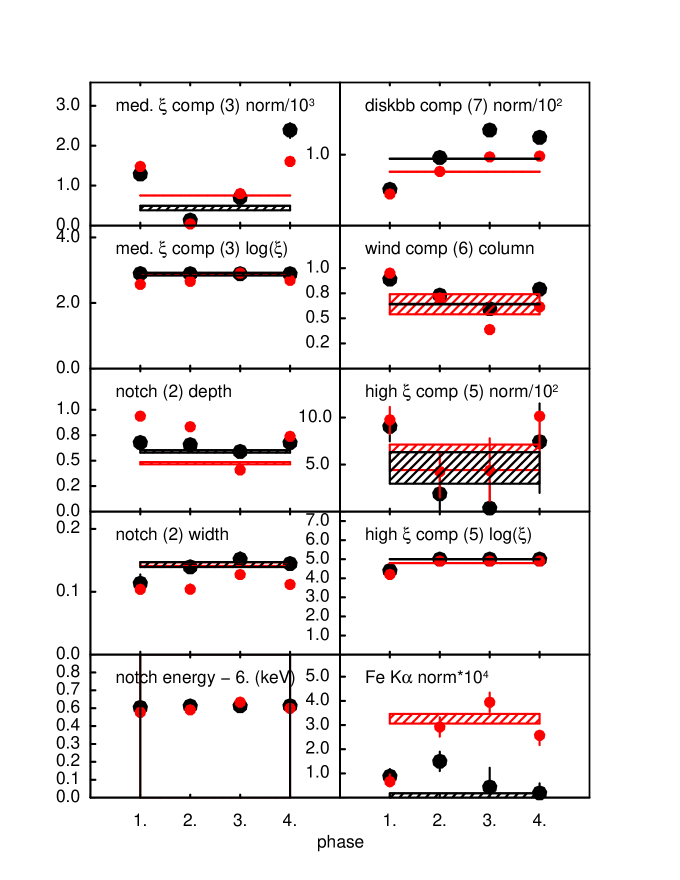
Figure 18.— Variation in spectral fit quantities with orbital phase. Hatched boxes show regions for phase average; black=Obsid_7268, red=Obsid_6601.

3.8. Obsid 16622

The data from obsids 425, 426 1456 and 16622, together with obsids 7268 and 6601, allow us to study the long term variability of Cyg X-3. Results of fitting to all the spectra, summed over the binary orbit, are given in table 7. This shows that obsids 7268 and 6601 correspond to the highest intensity states. Since they also have the longest observing times, they provide the most sensitive measurements of the various spectral components. Obsids 425 and 426 have intensities which are comparable, but with shorter observation times. Obside 16622 was obtained at the lowest flux state of all of these and differs significantly in its spectral properties. The flux during this observation was 2.15 $\times 10^{-8}$ erg cm^-2 s^-1 (89 mcrab) compared with $\sim$ 6 $\times 10^{-8}$ erg cm^-2 s^-1 ($\sim$240 mcrab) for the other obsids. Obsid 1456 was similar to Obsid 16622 in terms of state activity, and the observations have some features in common. However, the flux during Obsid 1456 is slightly less extreme than Obsid 16622, and also Obsid 1445 does not have as small statistical errors on measured spectral quantities, so we will base our subsequent discussion on Obsid 16622.

Principal differences between Obsid 16622 and the observations from higher flux states include a significantly harder continuum spectrum. We fit the other obsids with a 1.7 keV disk blackbody, which peaks at $\simeq$ 3.2 keV. Obsid 16622 requires a hard power law or a blackbody with kT=2 keV. The combination of this continuum and the neutral absorption causes the detected continuum to peak near 4.5 keV. In this sense, the contrast between this low flux state and the other obsids crudely resembles the difference between the low hard and high soft states of black hole transients.

In addition, the absorbing column for Obsid 16622 is lower, 2.28 $\times 10^{22}$ cm^-2 compared with 3.2 – 5.4 $\times 10^{22}$ cm^-2 for the other obsids. If much of the low energy absorption comes from the wind from the companion then this would suggest the companion as the source of this variability.

The line emission in Obsid 16622 crudely resembles that seen in other obsids in that the four line emitting components are all significantly detected, and with parameters similar to those found in the other fits. On the other hand, the the 6.4 keV iron K line has a similar flux compared with the other spectra, and therefore it has an equivalent width of 101$\pm$5 eV compared with 3 eV for Obsid 7268.

In addition, our model cannot adequately fit to Obsid 16622 using the same elemental abundances as used for all the other obsids. Those abundances included an enhancement of a factor 4 for the Si/Fe ratio, and a factor 2.6 for the S/Fe ratio compared with solar (Anders & Grevesse, 1989). These abundances greatly over-produce the Si and S lines when used in fitting to Obsid 16622, for which the best-fit Si/Fe ratio is $\sim$0.4 and the best-fit S/Fe ratio is $\sim$1 compared with solar. The abundances of Asplund et al. (2009) have Fe which is smaller than that of Anders & Grevesse (1989) by $\simeq$30$\%$, so all these ratios will be larger when interpreted in this context. These differences between fit results for different Obsids are indicative of shortcomings in the physical assumptions of our spectral model, since it is unlikely that the elemental abundances actually vary in this way. It is worth noting that WR winds are expected to have abundances which show evidence for nuclear processing. An example is the WN8 star analysis by Herald et al. (2001) which shows that Si and Ca are over-abundant and S, Ar, and Fe under-abundant compared to solar.

3.9. Long Term Variability

Figure 19 plots the parameters describing the various spectral components for the five obsids. These are plotted vs. the total flux in 2 - 10 keV band. This clearly shows that the medium $\xi$ nebular component 3 is strongest during the highest flux states, i.e. during obsids 6601 and 7268. The iron K$\alpha$ line shows the opposite behavior, and is strongest during low flux states. These results, together with the results of the phase resolved fitting in figure 18, suggest that the blackbody and the iron K$\alpha$ line are associated with gas close to the compact object. The nebular components are likely associated with the size scale of the binary orbit, and also are strongest when the source luminosity is greatest. This suggests that the X-ray luminosity of the source is determined by the wind from the star, i.e. the highest luminosity states coincide with the strongest wind. It also confirms the identification of the disk or accretion structure close to the compact object as the origin for the fluorescent K$\alpha$ line, and suggests that this feature and the associated accretion flow structure (i.e. the accretion disk) are anti-correlated with the wind from the companion.

Figure 19.— Variation in strengths of the various components plotted vs. flux in component 7, the diskbb continuum.

4. Discussion

The principal results obtained so far can be summarized as follows: (i) The He-like lines show that the centroid of the emission is not at the energy of the resonance or intercombination lines, but is rather between these two lines; (ii) The resonance line also shows blue-shifted absorption similar to a P-Cygni profile. This is similar to what is observed in the H-like lines (Vilhu et al., 2009). (iii) The He-like triplet intercombination and forbidden components are also present and are significantly narrower than the resonance line component. (iv) These results obtain in differing degrees for the He-like ions accessible to the Chandra HETG: Si, S, Ar, Ca. Iron differs in that the wind component is undetectable. (v) There is a trend that the wind component becomes weaker and possibly slower as the element atomic number increases, while the nebular component is consistent with having the same speed for all ions. For iron, it is possible that the wind is present but has a velocity which makes it indistiguishable from the narrower triplet lines. (vi) The density in the gas emitting the triplet component can be inferred from the R ratio, and it is consistent with a density greater than $10^{12}$ cm^-3. The R ratio for Ar is significantly greater, however, and this does not have an obvious explanation. (vii) Orbital-phase resolved spectra show that the nebular components are strongest close to eclipse transitions, while the dominant continuum component and iron K$\alpha$ line are strongest near inferior conjunction. (viii) Fitting to global models shows that the ionization balance of iron and lower Z elements cannot be modeled self-consistently; this could be due to absorption of the iron K emission from intermediate ion stages, or due to some ionization process which has not yet been explored. (ix) Comparison of spectra taken at different flux states reveals that, when the flux is low, the continuum is harder than in the other state and resembles a hard power law or hot blackbody.

4.1. Spherical Wind HMXB Models

It is of interest to compare the conditions implied by the observations with simple theoretical predictions for the HMXB winds. Such predictions were first explored by Hatchett & McCray (1977). In the simplest case, it is expected that the wind originates from the surface of the primary star and flows outward in spherical symmetry. The wind velocity starts with a value close to the sound speed at the photospheric temperature ($\sim 10^{5}$K), and accelerates to a terminal speed $\sim 1000$ km s^-1 within a few stellar radii. X-rays originate from the compact source and illuminate the wind. The ionization of the wind can be described by the ionization parameter $\xi=L/nr^{2}$, where $L$ is the X-ray source luminosity in the 1 - 1000 Ry energy range, $n$ is the gas density, and $r$ is the distance from the X-ray source. If so, the surfaces of constant $\xi$ are approximately spheres, nested around the X-ray source, or else open surfaces nested around the primary star. Which obtains depends on the quantity $q=\xi/\xi_{x}$, where $\xi_{x}=L/n_{x}a^{2}$ and $n_{x}$ is the wind density at the orbit of the compact object, and $a$ is the orbital separation. The $q=1$ surface is a plane dividing the orbital volume in half; closed surfaces surrounding the X-ray source have $q\geq$1. This is illustrated in figure 20.

It is straightforward to calculate the quantity of gas vs. ionization state using this simple model. The relevant quantity is the emission measure defined as $EM=\int{dVn^{2}}$ where $n$ is the nucleon density. The estimates depend on the properties of the wind and X-ray source. Here we adopt the following values: X-ray luminsity $L=2.5\times 10^{38}$ erg s^-1 (Vilhu et al., 2009); orbital separation $a=3.4R_{\odot}=2.37\times 10^{11}$ cm; primary radius $R_{*}=0.92R_{\odot}=6.4\times 10^{10}$ cm; wind mass loss rate $\dot{M}=10^{-5}M_{\odot}{\rm yr}^{-1}$; wind terminal speed $v_{\infty}=$1500 km s^-1. If so, the value for the predicted gas density near the X-ray source is $n_{x}\simeq 5.2\times 10^{12}$ cm^-3 and the fiducial ionization parameter is $\xi_{x}=8.6\times 10^{2}$ erg cm s^-1. This is the ionization parameter on the q=1 plane, i.e. the plane which bisects the binary volume. Thus, the X-ray source will produce an ionization parameter of this value or greater throughout its half-space, if the effects of attenuation are neglected. In the absence of X-ray ionization, the ionization balance in the wind is expected to resemble a $\sim 10^{5}$K coronal gas. That is, most elements will be 3 – 4 times ionized. Results of photoionization modeling (eg. Kallman et al. (2004)) shows that photoionization will increase the local ionization balance above that expected for a $\sim 10^{5}$K gas when $\xi\geq$10. Thus, the X-rays are expected to significantly change the wind ionization and temperature compared with that of a single WR star throughout more than half of the binary volume.

The total line emission from an effectively optically thin medium can be conveniently described by the luminosity $L_{line}=EMj/n^{2}$ where $EM$ is the emission measure and $j/n^{2}$ is the emissivity per nucleus. For a medium in which the temperature and ionization balance are constant throughout, the emission measure depends on the gas density distribution, and we can calculate it for various simple scenarios. Of course, the true emissivity is a function of temperature and ionization parameter, and so an accurate discussion must consider the distribution of emission measure over these quantities.

In the absence of X-rays, the wind is likely driven by UV radiation pressure from the primary. X-ray ionization will change the UV opacity of the wind, and therefore also affect the wind driving. Qualitatively, X-ray ionization will likely decrease the UV opacity, and hence the wind speed throughout the region where X-ray ionization is dominant. We can estimate where this occurs by assuming that the wind driving is cut off whenever the ionization parameter in the wind exceeds a critical value. Ionization of the wind by the compact source will cause the wind to be slower near the compact object and increase the mass accretion rate relative to the un-ionized wind (van den Heuvel et al., 2017).

For the parameter values chosen here, the $q=1$ surface occurs approximately 0.95 $R_{\odot}$ from the surface of the primary star; the density there is $n_{q=1}\simeq 2.5\times 10^{13}$ cm^-3. The surface where $\xi\simeq 10$, i.e. where the X-rays might be expected to affect the wind driving, occurs very close to the surface of the primary, at a distance of 0.06 $R_{\odot}$. The density there is 7.9 $\times 10^{14}$ cm^-3.

From the discussion in the previous section we can see that the emission measure needed to account for the observed lines is crudely $\sim 10^{60}$ cm^-3. The simple spherical wind model is expected to produce an emission measure which can be written $EM=\frac{(\dot{M}/\mu m_{H})^{2}}{4\pi av_{x}}F(q,a)$ where $F(q,a)$ is a function with value of order unity. Crudely, $EM=10^{59}\left(\frac{\dot{M}}{10^{-6}M_{\odot}/yr}\right)^{2}\left(\frac{a}{1.7\times 10^{12}{\rm cm}}\right)^{-1}\left(\frac{v_{x}}{1000{\rm kms}^{-1}}\right)^{-2}F(q,a){\rm cm}^{-3}$. Figure 21 shows the value of this quantity calculated numerically. The quantity plotted is the emission measure summed over all regions which have ionization parameters within bins of width 0.1 in log$\xi$, with the log$\xi$ value corresponding to the values on the horizontal axis of the figure. The simple spherical wind model produces emission measures which are greater than those implied by the observations, by a factor $\leq$10, at ionization parameters comparable to what we infer from the observed line strengths. This crude agreement suggests that the shadow wind + photoionized nebula explanation of the spectrum is not far from being correct. Closer agreement, if found, would likely be fortuitous, since the X-ray source almost certainly modifies the wind dynamics, either through its gravity or through its effect on the ionization and wind driving.

Figure 20.— Surfaces of constant q in the orbital plane. Axes are position in units of 10¹² cm. The companion star is shown as the dashed circle. The solid curve show surfaces of constant q. Black corresponds to q$\geq$1 and red corresponds to q$<$1. The X-ray source is at the center of the concentric black surfaces. This illustrates the fact that the X-ray source dominates the ionization throughout the half-space containing it.

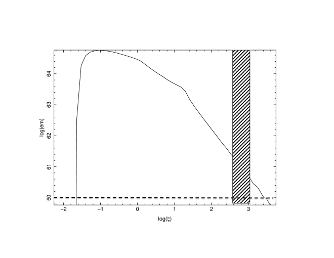
Figure 21.— Emission measure of an X-ray ionized wind with parameters similar to a single star Wolf-Rayet wind vs. ionization parameter. Values of EM and the range of $\xi$ for our nebular fits are shown as dashed and hatched regions, respectively.

4.2. Orbital Phase Dependence

The phase dependence of the continuum is crudely consistent with previous studies (Zdziarski et al., 2012), which suggests that absorption and scattering by the wind from the primary is the dominant process affecting the observed intensity. If so, the flux observed during the X-ray minimum is due to the partial transmission of the wind which occurs because the system inclination is not high enough to cause a complete eclipse of the source. However, we detect no significant change in the absorbing column with orbital phase. Such a change would be expected due to photoelectric absorption in the partially ionized wind material. Zdziarski et al. (2012) claim to find stronger orbital modulation at low energies in their analysis of RXTE, Swift, and Integral data. An alternative explanation for the broad band variability is that the disk is tilted or warped compared with the orbital plane. The disk would then be viewed at varying inclinations, and the foreshortening of the disk emission would account for the orbital variability.

As stated in the previous section, we can think about the results of the phase dependent spectral fits in terms of two sets of model components: those which are strongest in bins 1 and/or 4, and those which are strongest in bin 3. The former include the wind component 6, the high $\xi$ component 5, the medium $\xi$ component 3. The latter include the diskbb component 7, the iron K$\alpha$ component 4, and the notch component 2. During phase bins 1 and 4, the direct line of sight to the compact object is most obscured by the companion star wind. Thus, we attribute the components which are strongest at these phases to gas which is extended relative to the compact source. Such gas is likely associated with the companion wind, or the accretion flow on scales comparable to the binary separation. Thus, the X-ray wind component which we fit, and both the nebular emission components are likely to represent companion wind material which is ionized and whose dynamics are affected by the compact X-ray source. The wind component 6 is strongest as the system emerges from superior conjunction. Thus, if this is gas which is dynamically associated with the companion star, then it trails the star in its orbit. This is consistent with the expectation of a ’shadow wind’, as discussed in the following section. The medium $\xi$ component shows opposite behavior, for Obsid 7268, and is strongest as the system approaches superior conjunction. This suggests that it either leads the companion star in its orbit if it is dynamically associated with the companion star, or else it trails the compact object if it is associated with the compact object. In our phase-dependent fits we have held the windabs covering fraction constant. However, figures 10 and 11 show that the strength of the P-Cygni absorption in the Si¹²⁺ $r$ line and the Si¹³⁺ L$\alpha$ line appear to be stronger in phase bins 3 and 4. This suggests that the wind preferentially trails the companion star in its orbit, as expected for a shadow wind. This will be discussed in more detail below.

The components which are strongest in phase bin 3 we attribute to emission which is compact on the scale of the binary separation. Thus, the Fe K$\alpha$ line, the notch absorption, and the diskbb emission all fall in this category. These components all resemble components which are observed in other black hole candidate sources. If so, this system may resemble those, on scales much less than the binary separation. The notch absorption required by our fits could be attributed to a disk wind. If so, the fact that its depth is a maximum at phase bin 3 argues against orbital variability in the viewing angle of the disk, unless the disk is warped.

4.3. Shadow Wind

A spherical wind over-predicts the amount of material needed to account for the magnitude of the X-ray line emission in the Cyg X-3 system. It also does not provide a consistent explanation for the dynamical information we have derived from the spectrum. That is, we expect the X-ray source to ionize the wind above its mean ionization state throughout approximately half the wind volume. The lines accessible to $Chandra$ HETG observations correspond to an ionization state which is significantly higher than the mean ionization state the wind would have in the absence of X-ray ionization. We observe H- and He-like ions of elements as light as Si; the un-X-ray-ionized wind is expected to have 3-5 times ionized ions of Si and other elements. The dynamics of the wind depend on the ionization state, since the wind is thought to be driven by UV radiation pressure on lines in the ensemble of metal ions. H- and He-like ions have UV opacities with are much less than those of the 3-5 times ionized ions. Thus, we expect that the dynamics in the X-ray-ionized zone will be significantly different than in the un-ionized wind. In particular, there should be negligible wind driving, and the wind might be expected to ’coast’ in the X-ray ionized region.

The presence of P-Cygni lines in both He- and H-like lines appears to conflict with this scenario, in particular since the wind speed we measure is comparable to the full speed expected from a Wolf-Rayet wind. This suggests that the X-ray ionized gas has been accelerated as if it were not ionized beyond the wind background ionization level. A possible source for such gas is the ’shadow wind’ (Blondin, 1994), which is the wind formed in the region which is shadowed from X-ray ionization by the primary star. This wind is expected to have a velocity law which is unaffected by the X-rays. However, the rapid orbital motion of the system will bring this gas out of the shadow and expose it to X-ray ionization. The X-ray ionization timescale is expected to be $t_{ion}\simeq 4\pi\varepsilon/(n\xi\sigma_{PI})$ where $\sigma_{PI}$ is the photoionization cross section; this timescale is $\sim 10^{-3}$ s for plausible parameters. This can be compared with the flow timescale $t_{dyn}\sim a/v$, and this quantity has a value $\sim 10^{+3}$ s. Thus, the shadow wind will preserve its velocity structure as it becomes exposed to X-rays and shows X-ray ionized line features. The shadow wind is not spherical but rather resembles a narrow conical region which wraps around the star due to orbital motion. The shadow wind has been proposed as the origin for the variability in the strength of the IR lines by van Kerkwijk et al. (1996).

The windabs model fit provides the quantities needed to estimate the wind mass flux. The column density parameter values in tables 6 and 7 are log(column density/10²² cm^-2); typical parameter values in the range 0.4 – 0.9 correspond to column densities 2.5 – 8 $\times 10^{22}$ cm^-2. This corresponds to a wind mass loss rate approximately $\dot{M}_{wind}=0.8--2.6\times 10^{-7}M_{\odot}$ yr^-1 if the wind were spherical with the X-ray source at its center, and assuming an inner radius corresponding to the primary star, 6.4 $\times 10^{10}$ cm and a wind speed of 1600 km s^-1. Of course, these assumptions are not appropriate in this case, and do not account for the fact that the wind is demonstrably non-spherical. However, this value can be compared with the mass flux needed to fuel the X-ray source, which is $\dot{M}_{accretion}\simeq 4.1\times 10^{-8}M_{\odot}$ yr^-1 assuming a luminosity 2.46 $\times 10^{38}$ erg s^-1 and an efficiency of 0.1. This demonstrates that there is an adequate supply of gas in the wind to fuel the accretion unless the spherical estimate is too high by a factor $\geq$5.

An additional question is the origin of the nebular line emission. This gas has a velocity derived from line widths (sigma) which are a fraction of the value expected as the terminal velocity of the wind, approximately half. This therefore resembles the expectation for the gas which is accelerated in the wind region close to the primary star, where the density is high and the ionization parameter is low, and then coasts in the region where the X-ay source dominates the ionization. This scenario therefore provides a density measurement, via the He-like G ratio, which applies to the volume of the wind where the X-rays dominate.

4.4. Summary

The Chandra HETG spectrum of Cyg X-3 reveals rich detail in its variability and variety of emission mechansisms. Line emission originates from resonance scattering in a wind, whose dynamics are possibly associated with the UV/optical driven wind from the companion star. In addition there is emission from ’nebular’ gas, i.e. gas which is dominated by recombination and without the obvious kinematic signatures of a wind. There is potential confusion between one of the strongest features associated with the nebular component, i.e. the $f$ line of Si XIII at 1.84 keV, and the artifact of the scattering and absorption of X-rays by the K shell of Si in dust; simple models which attempt to simulate this process do not provide as good a fit as the models including nebular emission. The iron lines reveal a distinct component of gas at much higher ionization, and also a component from fluorescence by neutral or near-neutral material. Attempts to unify the iron emission with that of lower-Z elements implies a need for an additional absorption component, possibly associated with a disk wind. Variability with orbital phase reinforces the fact that these components are distinct. The wind and nebular components are anti-correlated with the peak of the continuum emission, suggesting an origin associated with the companion star. The fluorescence and iron-absorbing components are strongest when the continuum source is strongest, suggesting an association with the compact object. We have also examined the long term variability by comparing all the archival observations with significant exposure times. This shows that during X-ray low states a distinct continuum component emerges. We represent this by a 2 keV blackbody, though a hard power law can provide a comparable fit. This component is crudely anti-correlated with the total luminosity and the diskbb continuum. The iron K$\alpha$ line is also more prominent at low continuum flux. The wind and nebular components are likely associated with the size scale of the binary orbit, and also are strongest when the source luminosity is greatest. This suggests that the X-ray luminosity of the source is determined by the wind from the star, i.e. the highest luminosity states coincide with the strongest wind. It also confirms the identification of the disk or accretion structure close to the compact object as the origin for the fluorescent K$\alpha$ line and the blackbody, and suggests that these features and the associated accretion flow structure (i.e. the accretion disk) are anti-correlated with the wind from the companion.

Questions which are not resolved by our fits to these data include the origin, or other explanation, for the notch component 2. That is, what is responsible for the apparent absorption suppressing the K lines from intermediate stages of iron (i.e. L shell ions). In the previous sections we have discussed, and provisionally discarded, various possibilities associated with the ionization balance in the emitting gas. We have adopted a partially ionized absorbing wind explanation, though this raises additional questions, which we have not addressed, about the energetics, mass flux, and ionization of this wind.

Table 4Line IDs, wavelengths, widths and fluxes from Obsid 7268.

index	$\varepsilon$	$\lambda$	ion	lower level	upper level	ID	$\sigma$	Flux	voff
	keV	$\AA$					km s-1	cm-2 s-1	km s-1
1	$6.971^{+0.001}_{-0.001}$	$1.779^{+0.000}_{-0.000}$	fe_xxvi	1s1.2S_1/2	1s0.2p1.2P_3/2	L$\alpha$	$200.^{+8.}_{-8.}$	$2.2^{+0.1}_{-0.4}\times 10^{-3}$	90.
2	$6.948^{+0.003}_{-0.003}$	$1.784^{+0.004}_{-0.001}$	fe_xxvi	1s1.2S_1/2	1s0.2p1.2P_1/2	L$\alpha$	$192.^{+4.}_{-17.}$	$4.7^{+2.1}_{-1.1}\times 10^{-4}$	170.
3	$6.697^{+0.000}_{-0.000}$	$1.851^{+0.000}_{-0.000}$	fe_xxv	1s2.1S_0	1s1.2p1.1P_1	r	$198.^{+4.}_{-10.}$	$1.5^{+0.1}_{-0.5}\times 10^{-3}$	140.
4	$6.669^{+0.001}_{-0.001}$	$1.859^{+0.000}_{-0.000}$	fe_xxv	1s2.1S_0	1s1.2p1.3P_1	i	$200.^{+2.}_{-50.}$	$2.5^{+0.0}_{-1.1}\times 10^{-3}$	-50.
5	$6.641^{+0.001}_{-0.001}$	$1.867^{+0.000}_{-0.000}$	fe_xxv	1s2.1S_0	1s1.2s1.3S_1	f	$198.^{+2.}_{-62.}$	$1.1^{+0.3}_{-0.1}\times 10^{-3}$	-190.
6	$5.133^{+0.014}_{-0.014}$	$2.416^{+0.001}_{-0.006}$	ca_xx	1s1.2S_1/2	1s0.4p1.2P_3/2	L$\gamma$	$199.^{+92.}_{-75.}$	$2.8^{+1.0}_{-1.0}\times 10^{-4}$	-190.
7	$4.867^{+0.002}_{-0.002}$	$2.547^{+0.001}_{-0.001}$	ca_xx	1s1.2S_1/2	1s0.3p1.2P_3/2	L$\beta$	$200.^{+37.}_{-23.}$	$4.6^{+0.8}_{-1.3}\times 10^{-4}$	-190.
8	$4.859^{+0.020}_{-0.019}$	$2.552^{+0.007}_{-0.010}$	ca_xx	1s1.2S_1/2	1s0.3p1.2P_1/2	L$\beta$	$200.^{+23.}_{-31.}$	$2.4^{+1.0}_{-0.0}\times 10^{-4}$	190.
9	$4.825^{+0.013}_{-0.013}$	$2.570^{+0.002}_{-0.007}$	ca_xix	1s2.1S_0	1s1.4p1.1P_1	1 - 3	$200.^{+25.}_{-28.}$	$3.0^{+0.8}_{-1.2}\times 10^{-4}$	-180.
10	$4.580^{+0.001}_{-0.001}$	$2.707^{+0.003}_{-0.001}$	ca_xix	1s2.1S_0	1s1.3p1.1P_1	1 - 3	$199.^{+25.}_{-21.}$	$5.7^{+0.9}_{-1.1}\times 10^{-4}$	190.
11	$4.148^{+0.001}_{-0.001}$	$2.989^{+0.003}_{-0.001}$	ar_xvii	1s1.2S_1/2	1s0.4p1.2P_3/2	L$\gamma$	$116.^{+62.}_{-29.}$	$4.7^{+0.5}_{-0.7}\times 10^{-4}$	190.
12	$4.105^{+0.000}_{-0.000}$	$3.020^{+0.004}_{-0.000}$	ca_xx	1s1.2S_1/2	1s0.2p1.2P_3/2	L$\alpha$	$200.^{+8.}_{-17.}$	$1.7^{+0.1}_{-0.1}\times 10^{-3}$	150.
13	$4.097^{+0.000}_{-0.000}$	$3.026^{+0.008}_{-0.000}$	ca_xx	1s1.2S_1/2	1s0.2p1.2P_1/2	L$\alpha$	$200.^{+2.}_{-57.}$	$7.5^{+0.9}_{-1.4}\times 10^{-4}$	200.
14	$3.935^{+0.001}_{-0.001}$	$3.151^{+0.001}_{-0.001}$	ar_xvii	1s1.2S_1/2	1s0.3p1.2P_3/2	L$\beta$	$200.^{+42.}_{-24.}$	$5.2^{+1.1}_{-1.0}\times 10^{-4}$	30.
15	$3.933^{+0.011}_{-0.011}$	$3.153^{+0.013}_{-0.008}$	ar_xvii	1s1.2S_1/2	1s0.3p1.2P_1/2	L$\beta$	$138.^{+35.}_{-28.}$	$2.0^{+0.7}_{-0.0}\times 10^{-4}$	100.
16	$3.902^{+0.000}_{-0.000}$	$3.177^{+0.001}_{-0.000}$	ca_xix	1s2.1S_0	1s1.2p1.1P_1	r	$194.^{+30.}_{-6.}$	$1.5^{+0.1}_{-0.1}\times 10^{-3}$	10.
17	$3.890^{+0.000}_{-0.000}$	$3.187^{+0.007}_{-0.000}$	ca_xix	1s2.1S_0	1s1.2p1.3P_2	i	$200.^{+10.}_{-13.}$	$9.1^{+1.0}_{-1.3}\times 10^{-4}$	-190.
18	$3.883^{+0.000}_{-0.000}$	$3.193^{+0.009}_{-0.000}$	ca_xix	1s2.1S_0	1s1.2p1.3P_1	i	$199.^{+4.}_{-31.}$	$2.0^{+0.6}_{-1.9}\times 10^{-4}$	60.
19	$3.872^{+0.000}_{-0.000}$	$3.202^{+0.007}_{-0.000}$	ar_xvii	1s2.1S	1s1.4p1.1P	1 - 4	$199.^{+2.}_{-44.}$	$10.0^{+1.2}_{-1.0}\times 10^{-4}$	190.
20	$3.861^{+0.002}_{-0.002}$	$3.211^{+0.002}_{-0.002}$	ca_xix	1s2.1S_0	1s1.2s1.3S_1	f	$199.^{+2.}_{-49.}$	$3.9^{+1.3}_{-0.8}\times 10^{-4}$	20.
21	$3.682^{+0.002}_{-0.002}$	$3.367^{+0.002}_{-0.002}$	ar_xvii	1s2.1S	1s1.3p1.1P	1 - 3	$199.^{+2.}_{-49.}$	$3.4^{+1.0}_{-1.1}\times 10^{-4}$	140.
22	$3.321^{+0.000}_{-0.000}$	$3.733^{+0.003}_{-0.000}$	ar_xvii	1s1.2S_1/2	1s0.2p1.2P_3/2	L$\alpha$	$195.^{+28.}_{-6.}$	$2.3^{+0.1}_{-0.2}\times 10^{-3}$	160.
23	$3.316^{+0.000}_{-0.000}$	$3.739^{+0.009}_{-0.000}$	ar_xvii	1s1.2S_1/2	1s0.2p1.2P_1/2	L$\alpha$	$193.^{+2.}_{-46.}$	$9.2^{+1.2}_{-1.3}\times 10^{-4}$	190.
24	$3.275^{+0.001}_{-0.001}$	$3.786^{+0.001}_{-0.001}$	s_xvi	1s1.2S_1/2	1s0.4p1.2P_3/2	L$\gamma$	$198.^{+2.}_{-42.}$	$6.4^{+1.2}_{-1.2}\times 10^{-4}$	100.
25	$3.137^{+0.000}_{-0.000}$	$3.952^{+0.005}_{-0.000}$	ar_xvii	1s2.1S	1s1.2p1.1P	r	$200.^{+2.}_{-34.}$	$1.1^{+0.1}_{-0.1}\times 10^{-3}$	190.
26	$3.127^{+0.003}_{-0.003}$	$3.965^{+0.000}_{-0.004}$	ar_xvii	1s2.1S	1s1.2p1.3P	i	$200.^{+2.}_{-36.}$	$7.5^{+1.7}_{-0.9}\times 10^{-4}$	-190.
27	$3.107^{+0.000}_{-0.000}$	$3.990^{+0.001}_{-0.001}$	s_xvi	1s1.2S_1/2	1s0.3p1.2P_3/2	L$\beta$	$199.^{+2.}_{-28.}$	$1.6^{+0.1}_{-0.1}\times 10^{-3}$	-20.
28	$3.104^{+0.000}_{-0.000}$	$3.995^{+0.011}_{-0.000}$	ar_xvii	1s2.1S	1s1.2s1.3S	f	$199.^{+2.}_{-34.}$	$1.1^{+12.6}_{-12.7}\times 10^{-5}$	50.
29	$3.099^{+0.000}_{-0.000}$	$4.001^{+0.007}_{-0.000}$	s_xv	1s2.1S_0	1s1.5p1.1P_1	1 - 5	$200.^{+2.}_{-39.}$	$6.5^{+1.3}_{-1.2}\times 10^{-4}$	190.
30	$2.621^{+0.000}_{-0.000}$	$4.731^{+0.009}_{-0.000}$	s_xvi	1s1.2S_1/2	1s0.2p1.2P_3/2	L$\alpha$	$200.^{+70.}_{-6.}$	$4.2^{+0.4}_{-0.4}\times 10^{-3}$	190.
31	$2.618^{+0.000}_{-0.000}$	$4.736^{+0.010}_{-0.000}$	s_xvi	1s1.2S_1/2	1s0.2p1.2P_1/2	L$\alpha$	$200.^{+2.}_{-62.}$	$2.1^{+0.4}_{-0.3}\times 10^{-3}$	190.
32	$2.505^{+0.001}_{-0.001}$	$4.950^{+0.013}_{-0.003}$	si_xiv	1s1.2S_1/2	1s0.4p1.2P_3/2	L$\gamma$	$200.^{+2.}_{-62.}$	$1.5^{+2.0}_{-0.0}\times 10^{-4}$	190.
33	$2.459^{+0.000}_{-0.000}$	$5.042^{+0.014}_{-0.000}$	s_xv	1s2.1S_0	1s1.2p1.1P_1	r	$200.^{+83.}_{-13.}$	$1.4^{+0.2}_{-0.2}\times 10^{-3}$	200.
34	$2.450^{+0.004}_{-0.004}$	$5.060^{+0.000}_{-0.009}$	s_xv	1s2.1S_0	1s1.2p1.3P_2	i	$200.^{+51.}_{-10.}$	$1.5^{+0.2}_{-0.2}\times 10^{-3}$	-190.
35	$2.445^{+0.000}_{-0.000}$	$5.070^{+0.014}_{-0.001}$	s_xv	1s2.1S_0	1s1.2p1.3P_1	i	$200.^{+23.}_{-13.}$	$4.2^{+2.0}_{-1.8}\times 10^{-4}$	190.
36	$2.432^{+0.001}_{-0.001}$	$5.098^{+0.003}_{-0.002}$	s_xv	1s2.1S_0	1s1.2s1.3S_1	f	$200.^{+14.}_{-19.}$	$4.0^{+2.1}_{-2.1}\times 10^{-4}$	-190.
37	$2.375^{+0.000}_{-0.000}$	$5.220^{+0.009}_{-0.000}$	si_xiv	1s1.2S_1/2	1s0.3p1.2P_3/2	L$\beta$	$200.^{+14.}_{-17.}$	$8.8^{+2.4}_{-2.2}\times 10^{-4}$	200.
38	$2.005^{+0.000}_{-0.000}$	$6.185^{+0.008}_{-0.000}$	si_xiv	1s1.2S_1/2	1s0.2p1.2P_3/2	L$\alpha$	$200.^{+81.}_{-2.}$	$6.4^{+0.3}_{-0.3}\times 10^{-3}$	200.
39	$2.003^{+0.000}_{-0.000}$	$6.190^{+0.017}_{-0.000}$	si_xiv	1s1.2S_1/2	1s0.2p1.2P_1/2	L$\alpha$	$200.^{+2.}_{-34.}$	$2.2^{+0.2}_{-0.5}\times 10^{-3}$	200.
40	$1.883^{+0.001}_{-0.001}$	$6.583^{+0.003}_{-0.003}$	mg_xii	1s1.2S_1/2	1s0.5p1.2P_3/2	L$\delta$	$198.^{+6.}_{-39.}$	$2.6^{+2.1}_{-2.0}\times 10^{-4}$	130.
41	$1.864^{+0.000}_{-0.000}$	$6.652^{+0.018}_{-0.000}$	si_xiii	1s2.1S_0	1s1.2p1.1P_1	r	$199.^{+10.}_{-24.}$	$1.4^{+0.3}_{-0.3}\times 10^{-3}$	190.
42	$1.856^{+0.005}_{-0.005}$	$6.681^{+0.001}_{-0.018}$	si_xiii	1s2.1S_0	1s1.2p1.3P_2	i	$198.^{+76.}_{-3.}$	$3.2^{+6.9}_{-1.5}\times 10^{-4}$	-190.
43	$1.853^{+0.000}_{-0.000}$	$6.693^{+0.018}_{-0.001}$	si_xiii	1s2.1S_0	1s1.2p1.3P_1	i	$199.^{+76.}_{-3.}$	$2.2^{+4.7}_{-2.3}\times 10^{-4}$	190.
44	$1.840^{+0.000}_{-0.000}$	$6.737^{+0.001}_{-0.001}$	mg_xii	1s1.2S_1/2	1s0.4p1.2P_3/2	L$\gamma$	$200.^{+14.}_{-12.}$	$2.3^{+0.2}_{-0.4}\times 10^{-3}$	-30.
45	$1.839^{+0.000}_{-0.000}$	$6.743^{+0.011}_{-0.001}$	mg_xii	1s1.2S_1/2	1s0.4p1.2P_1/2	L$\gamma$	$200.^{+6.}_{-23.}$	$2.6^{+2.0}_{-2.0}\times 10^{-4}$	190.
46	$1.745^{+0.000}_{-0.000}$	$7.105^{+0.002}_{-0.002}$	mg_xii	1s1.2S_1/2	1s0.3p1.2P_3/2	L$\beta$	$200.^{+8.}_{-19.}$	$7.4^{+6.1}_{-1.0}\times 10^{-4}$	-50.
47	$1.743^{+0.002}_{-0.002}$	$7.112^{+0.019}_{-0.009}$	mg_xii	1s1.2S_1/2	1s0.3p1.2P_1/2	L$\beta$	$200.^{+8.}_{-19.}$	$2.3^{+2.6}_{-2.2}\times 10^{-4}$	190.
48	$1.728^{+0.000}_{-0.000}$	$7.176^{+0.008}_{-0.001}$	al_xiii	1s1.2S_1/2	1s0.2p1.2P_3/2	L$\alpha$	$200.^{+10.}_{-13.}$	$1.4^{+0.2}_{-0.3}\times 10^{-3}$	200.
49	$1.599^{+0.001}_{-0.001}$	$7.752^{+0.029}_{-0.004}$	al_xii	1s2.1S_0	1s1.2p1.1P_1	r	$200.^{+14.}_{-10.}$	$1.7^{+0.3}_{-0.6}\times 10^{-3}$	-190.
50	$1.472^{+0.000}_{-0.000}$	$8.420^{+0.002}_{-0.002}$	mg_xii	1s1.2S_1/2	1s0.2p1.2P_3/2	L$\alpha$	$200.^{+672.}_{-4.}$	$8.0^{+1.4}_{-0.7}\times 10^{-3}$	30.
51	$1.471^{+0.000}_{-0.000}$	$8.430^{+0.023}_{-0.000}$	mg_xii	1s1.2S_1/2	1s0.2p1.2P_1/2	L$\alpha$	$200.^{+146.}_{-8.}$	$2.3^{+0.8}_{-1.0}\times 10^{-3}$	190.
52	$1.351^{+0.000}_{-0.000}$	$9.175^{+0.025}_{-0.002}$	mg_xi	1s2.1S_0	1s1.2p1.1P_1	r	$200.^{+235.}_{-4.}$	$8.9^{+1.9}_{-2.1}\times 10^{-3}$	190.
53	$1.344^{+0.001}_{-0.001}$	$9.222^{+0.001}_{-0.009}$	mg_xi	1s2.1S_0	1s1.2p1.3P_2	i	$200.^{+257.}_{-2.}$	$1.2^{+0.3}_{-0.2}\times 10^{-2}$	-190.
54	$1.342^{+0.000}_{-0.000}$	$9.237^{+0.025}_{-0.001}$	mg_xi	1s2.1S_0	1s1.2p1.3P_1	i	$200.^{+226.}_{-2.}$	$2.0^{+4.6}_{-0.7}\times 10^{-3}$	200.
55	$1.331^{+0.001}_{-0.001}$	$9.315^{+0.005}_{-0.007}$	mg_xi	1s2.1S_0	1s1.2s1.3S_1	f	$200.^{+305.}_{-2.}$	$1.0^{+1.0}_{-0.1}\times 10^{-2}$	-30.
56	$1.168^{+0.003}_{-0.003}$	$10.612^{+0.019}_{-0.028}$	fe_xxiv	2s1.2S_1/2	2s0.3p1.2P_3/2		$200.^{+330.}_{-2.}$	$9.2^{+99.7}_{-3.0}\times 10^{-3}$	-190.
57	$1.163^{+0.001}_{-0.001}$	$10.661^{+0.036}_{-0.012}$	fe_xxiv	2s1.2S_1/2	2s0.3p1.2P_1/2		$200.^{+341.}_{-2.}$	$9.2^{+114.5}_{-3.2}\times 10^{-3}$	-50.

Table 5RRC wavelengths, IDs, widths and fluxes.

index	$\varepsilon$	$\lambda$	ion	lower level	upper level	ID	kT	Flux	voff
	keV	$\AA$					km s-1	cm-2 s-1	km s-1
1	$5.126^{+0.021}_{-0.020}$	$2.419^{+0.006}_{-0.010}$	ca_xix	1s2.1S_0	continuum	RRC	$199.^{+62.}_{-84.}$	$6.8^{+18.8}_{-0.0}\times 10^{-5}$	190.
2	$4.424^{+0.001}_{-0.001}$	$2.802^{+0.000}_{-0.000}$	ar_xvii	1s1.2S_1/2	continuum	RRC	$199.^{+213.}_{-136.}$	$4.0^{+1.1}_{-1.0}\times 10^{-4}$	100.
3	$4.119^{+0.000}_{-0.000}$	$3.010^{+0.000}_{-0.000}$	ar_xvii	1s2.1S	continuum	RRC	$103.^{+918.}_{-4.}$	$4.5^{+0.3}_{-1.0}\times 10^{-4}$	120.
4	$3.226^{+0.010}_{-0.010}$	$3.844^{+0.001}_{-0.012}$	s_xv	1s2.1S_0	continuum	RRC	$197.^{+2.}_{-44.}$	$2.2^{+1.6}_{-1.5}\times 10^{-4}$	-170.
5	$2.674^{+0.007}_{-0.007}$	$4.636^{+0.001}_{-0.013}$	si_xiv	1s1.2S_1/2	continuum	RRC	$200.^{+49.}_{-84.}$	$1.1^{+0.5}_{-0.6}\times 10^{-3}$	-140.
6	$2.438^{+0.000}_{-0.000}$	$5.085^{+0.000}_{-0.001}$	si_xiii	1s2.1S_0	continuum	RRC	$200.^{+25.}_{-12.}$	$1.5^{+0.3}_{-0.3}\times 10^{-3}$	-30.
7	$1.998^{+0.000}_{-0.000}$	$6.205^{+0.000}_{-0.000}$	fe_xxiv	2s0.2p1.2P_1/2	continuum	RRC	$155.^{+6.}_{-39.}$	$3.4^{+0.2}_{-0.5}\times 10^{-3}$	-110.
8	$1.855^{+0.000}_{-0.000}$	$6.682^{+0.000}_{-0.001}$	fe_xxii	2s1.2p1.1P_1	continuum	RRC	$200.^{+12.}_{-19.}$	$2.4^{+0.4}_{-0.4}\times 10^{-3}$	180.
9	$1.674^{+0.000}_{-0.000}$	$7.408^{+0.002}_{-0.000}$	fe_xxi	2p2.3P_2	continuum	RRC	$200.^{+10.}_{-12.}$	$1.8^{+0.8}_{-0.8}\times 10^{-3}$	120.
10	$1.642^{+0.000}_{-0.000}$	$7.552^{+0.008}_{-0.002}$	fe_xxi	2p2.1S_0	continuum	RRC	$200.^{+12.}_{-12.}$	$1.0^{+0.6}_{-0.6}\times 10^{-3}$	200.
11	$1.583^{+0.000}_{-0.000}$	$7.832^{+0.001}_{-0.000}$	fe_xx	2p3.4S_3/2	continuum	RRC	$200.^{+14.}_{-10.}$	$3.5^{+1.0}_{-0.9}\times 10^{-3}$	-180.
12	$1.566^{+0.000}_{-0.000}$	$7.919^{+0.001}_{-0.000}$	fe_xx	2p3.2D_3/2	continuum	RRC	$200.^{+19.}_{-6.}$	$5.0^{+1.1}_{-1.0}\times 10^{-3}$	-160.
13	$1.543^{+0.000}_{-0.000}$	$8.036^{+0.001}_{-0.001}$	fe_xx	2p3.2P_3/2	continuum	RRC	$200.^{+21.}_{-6.}$	$3.4^{+1.1}_{-0.7}\times 10^{-3}$	-190.
14	$1.457^{+0.000}_{-0.000}$	$8.512^{+0.001}_{-0.000}$	fe_xix	2p4.3P_2	continuum	RRC	$199.^{+205.}_{-4.}$	$1.1^{+0.2}_{-0.2}\times 10^{-2}$	-120.
15	$1.446^{+0.000}_{-0.000}$	$8.576^{+0.001}_{-0.000}$	fe_xix	2p4.3P_0	continuum	RRC	$199.^{+218.}_{-4.}$	$1.1^{+0.2}_{-0.2}\times 10^{-2}$	190.
16	$1.444^{+0.000}_{-0.000}$	$8.587^{+0.023}_{-0.001}$	fe_xix	2p4.3P_1	continuum	RRC	$198.^{+190.}_{-4.}$	$1.3^{+6.8}_{-0.3}\times 10^{-3}$	190.
17	$1.246^{+0.000}_{-0.000}$	$9.947^{+0.000}_{-0.002}$	ca_xix	1s1.2p1.3P_0	continuum	RRC	$200.^{+315.}_{-2.}$	$9.8^{+40.2}_{-2.4}\times 10^{-3}$	70.
18	$1.245^{+0.004}_{-0.004}$	$9.957^{+0.036}_{-0.030}$	ca_xix	1s1.2s1.1S_0	continuum	RRC	$200.^{+320.}_{-2.}$	$9.8^{+16.9}_{-5.2}\times 10^{-3}$	-90.

Table 6Parameters for Global Fit, Nebula plus Wind, Phase-Summed Spectra

component	parameter	Obsid_6601	Obsid_1456000	Obsid_1456002	Obsid_425	Obsid_16622	Obsid_426	Obsid_7268
1	NH	4.25${}_{-0.01}^{+0.01}$	3.75${}_{-0.05}^{+0.04}$	4.02${}_{-0.10}^{+0.09}$	5.68${}_{-0.02}^{+0.03}$	2.28${}_{-0.07}^{+0.06}$	5.34${}_{-0.03}^{+0.03}$	4.16${}_{-0.01}^{+0.01}$
2	notch energy - 6. (keV)	0.56${}_{-6.00}^{+-6.00}$	0.55${}_{-6.00}^{+-6.00}$	0.55${}_{-6.00}^{+-6.00}$	0.55${}_{-6.00}^{+-6.00}$	0.50${}_{-6.00}^{+-6.00}$	0.55${}_{-6.00}^{+-6.00}$	0.57${}_{-6.00}^{+-6.00}$
3	notch (2) width	0.16	0.10	0.10	0.10		0.10	0.16
4	notch (2) depth	0.47${}_{-0.01}^{+0.01}$	0.58${}_{-0.03}^{+0.03}$	0.68${}_{-0.03}^{+0.03}$	0.58${}_{-0.03}^{+0.03}$	$\leq$ 0.04	0.58${}_{-0.03}^{+0.03}$	0.59${}_{-0.01}^{+0.01}$
5	mga,b	7.58${}_{-0.07}^{+0.06}$
6	al	6.16${}_{-0.23}^{+0.15}$
7	si	8.06${}_{-0.01}^{+0.01}$
8	s	7.67${}_{-0.03}^{+0.04}$
9	ar	7.14${}_{-0.06}^{+0.05}$
10	ca	7.19${}_{-0.15}^{+0.06}$
11	fe	8.27
12	z	0.001
13	medium $\xi$ comp (3) log($\xi$)c	2.90${}_{-0.01}^{+0.01}$	2.90	2.90	2.90	2.20	2.90	2.89${}_{-0.05}^{+0.03}$
14	medium $\xi$ comp (3) normd	0.75${}_{0.00}^{+0.00}$	0.25${}_{0.00}^{+0.03}$	0.41${}_{-0.05}^{+0.05}$	0.97${}_{-0.06}^{+0.06}$	$\leq$ 0.01	0.97${}_{-0.09}^{+0.09}$	0.43${}_{-0.05}^{+0.06}$
15	Fe K$\alpha$ norm*104e	3.26${}_{-0.20}^{+0.20}$	3.45${}_{-0.27}^{+0.28}$	3.05${}_{-0.30}^{+0.31}$	2.50${}_{-0.32}^{+0.33}$	4.30${}_{-0.26}^{+0.28}$	2.52${}_{-0.35}^{+0.35}$	$\leq$ 0.18
16	high $\xi$ comp (5) log($\xi$)c	4.80	4.50	5.00	5.00	4.20	5.00	5.00
17	high $\xi$ comp (5) norm/102d	5.85${}_{-1.44}^{+1.28}$	4.83${}_{-2.16}^{+0.65}$	5.00${}_{-2.44}^{+2.09}$	8.49${}_{-2.85}^{+2.89}$	11.43 ${}_{-0.19}^{+0.20}$	8.49${}_{-3.55}^{+3.59}$	4.63${}_{-1.66}^{+1.68}$
18	wind comp (6) columnf	0.64${}_{-0.10}^{+0.10}$	0.89${}_{-0.10}^{+0.10}$	1.10${}_{-0.10}^{+0.10}$	0.89${}_{-0.10}^{+0.10}$	-0.23${}_{-0.10}^{+0.10}$	0.89${}_{-0.10}^{+0.10}$	0.64
19	vturb (km s-1)	1600.00
20	cfrac	1.80
21	zwind	0.001
22	tin	1.72
23	diskbb comp (7) normg	0.76	0.07	0.05	0.13${}_{0.00}^{+0.01}$		0.13	0.94
24	kT (8)	2.00	1.97	2.39	1.34	2.00	1.34	2.00
25	blackbody norm*102g		2.81${}_{-0.05}^{+0.07}$	2.49${}_{-0.10}^{+0.11}$	9.55${}_{-0.10}^{+0.03}$	3.89${}_{-0.04}^{+0.04}$	9.55${}_{-0.21}^{+0.16}$	1.29${}_{-0.06}^{+0.06}$
26	cstat	61824.94	15565.53	13101.69	21325.52	13387.40	21325.50	214748.36
27	dof	32761.00	32761.00	32761.00	32761.00	32761.00	32761.00	32761.00
28	chisq	68105.80	7344.08	4871.88	14424.98	5068.53	14425.15	65343.20
29	flux/100 mCrab	2.53	0.83	0.60	2.55	0.86	2.33	3.44
30	tobs	49200.00	12100.00	8419.00	18959.77	28625.00	15700.00	69900.00

Table 7Parameters for Global Fit, Nebula plus Wind, Phase-binned Spectra

component	parameter	7268 phase 1	7268 phase 2	7268 phase 3	7268 phase 4	6601 phase 1	6601 phase 2	6601 phase 3	6601 phase 4
1	NH	4.09${}_{-0.02}^{+0.02}$	4.40${}_{-0.01}^{+0.01}$	4.20${}_{-0.01}^{+0.01}$	4.30${}_{-0.01}^{+0.01}$	4.17${}_{-0.02}^{+0.02}$	4.36${}_{-0.01}^{+0.01}$	4.01${}_{-0.01}^{+0.01}$	3.90
2	notch energy - 6. (keV)	0.56${}_{-6.01}^{+-6.00}$	0.57${}_{-6.00}^{+-6.00}$	0.57${}_{-6.01}^{+-6.00}$	0.57${}_{-6.00}^{+-6.00}$	0.53${}_{-6.00}^{+-6.00}$	0.55${}_{-6.00}^{+-6.00}$	0.59${}_{-6.00}^{+-6.00}$	0.55${}_{-6.00}^{+-6.00}$
3	notch (2) width	0.13${}_{-0.01}^{+0.02}$	0.16${}_{-0.01}^{+0.01}$	0.17${}_{-0.01}^{+0.01}$	0.16${}_{-0.01}^{+0.01}$	0.12${}_{-0.01}^{+0.01}$	0.12${}_{-0.01}^{+0.01}$	0.14${}_{-0.01}^{+0.01}$	0.12
4	notch (2) depth	0.68${}_{-0.04}^{+0.03}$	0.66${}_{-0.02}^{+0.02}$	0.59${}_{0.02}^{+0.02}$	0.68${}_{-0.02}^{+0.01}$	0.94${}_{-0.03}^{+0.02}$	0.83${}_{-0.03}^{+0.03}$	0.41${}_{-0.02}^{+0.02}$	0.74
5	mga,b	7.58${}_{-0.07}^{+0.06}$
6	al	6.16${}_{-0.23}^{+0.15}$
7	si	8.06${}_{-0.01}^{+0.01}$
8	s	7.67${}_{-0.03}^{+0.04}$
9	ar	7.14${}_{-0.06}^{+0.05}$
10	ca	7.19${}_{-0.15}^{+0.06}$
11	fe	8.27
12	z	0.001
13	medium $\xi$ comp (3) log($\xi$)c	2.89	2.89${}_{-0.07}^{+0.01}$	2.89${}_{-0.07}^{+0.01}$	2.89${}_{-0.05}^{+0.03}$	2.57	2.66	2.91	2.69
14	medium $\xi$ comp (3) normd	1.29${}_{0.00}^{+0.01}$	0.13${}_{0.00}^{+0.02}$	0.70${}_{0.00}^{+0.04}$	2.39${}_{-0.19}^{+0.17}$	1.48${}_{0.00}^{+0.08}$	0.04 ${}_{0.00}^{+0.01}$	0.80${}_{-0.09}^{+0.09}$	1.60
15	Fe K$\alpha$ norm*104e	0.88${}_{-0.30}^{+0.30}$	1.50${}_{-0.40}^{+0.40}$	0.44${}_{0.00}^{+0.80}$	0.19${}_{0.40}^{+0.40}$	0.66${}_{-0.20}^{+0.30}$	2.92${}_{-0.40}^{+0.40}$	3.94${}_{-0.40}^{+0.40}$	2.57
16	high $\xi$ comp (5) log($\xi$)c	4.40	5.00	5.00	5.00	4.20	4.90	4.90	4.90
17	high $\xi$ comp (5) norm/102d	9.05${}_{-1.59}^{+1.04}$	1.88${}_{-1.46}^{+2.22}$	0.36${}_{-0.76}^{+2.83}$	7.43${}_{-5.44}^{+4.07}$	9.75${}_{-1.51}^{+1.37}$	4.25${}_{-2.74}^{+2.10}$	4.36${}_{-3.25}^{+3.43}$	10.14
18	wind comp (6) columnf	0.89${}_{-0.00}^{+0.01}$	0.73${}_{-0.02}^{+0.03}$	0.60${}_{-0.02}^{+0.03}$	0.79${}_{-0.02}^{+0.02}$	0.95	0.70	0.39	0.61
19	vturb	1600.0
20	cfrac	1.80
21	zwind	0.001
22	tin	1.72
23	diskbb comp (7) normg	0.51	0.96	1.35	1.24	0.44	0.76	0.97	0.98
24	kT (8)	2.00
25	blackbody norm*102g
26	cstat	59227.92	66186.24	65288.02	65198.33	21812.77	2257.27	29146.67	27815.88
27	dof	32761.00	32761.00	32761.00	32761.00	32761.00	32761.00	32761.00	32761.00
28	chisq	16371.30	19699.67	21359.17	21462.95	12296.02	15580.80	22375.15	214748.36
29	flux/100 mCrab	1.68	3.06	4.44	3.96	1.28	2.36	3.31	3.20

References

- Al-Malki et al. (1999) Al-Malki, M. B., Simmons, J. F. L., Ignace, R., Brown, J. C., & Clarke, D. 1999, A&A, 347, 919
- Anders & Grevesse (1989) Anders, E., & Grevesse, N. 1989, Geochim. Cosmochim. Acta, 53, 197
- Arnaud (1996) Arnaud, K. A. 1996, Astronomical Data Analysis Software and Systems V, 101, 17
- Asplund et al. (2009) Asplund, M., Grevesse, N., Sauval, A. J., & Scott, P. 2009, ARA&A, 47, 481
- Avni (1976) Avni, Y. 1976, ApJ, 210, 642
- Bautista & Kallman (2000) Bautista, M. A., & Kallman, T. R. 2000, ApJ, 544, 581
- Bhargava et al. (2017) Bhargava, Y., Rao, A. R., Singh, K. P., et al. 2017, ApJ, 849, 141
- Blondin (1994) Blondin, J. M. 1994, ApJ, 435, 756
- Cash (1979) Cash, W. 1979, ApJ, 228, 939
- Corrales & Paerels (2015) Corrales, L. R., & Paerels, F. 2015, MNRAS, 453, 1121
- Corrales et al. (2016) Corrales, L. R., García, J., Wilms, J., & Baganoff, F. 2016, MNRAS, 458, 1345
- Draine (2003) Draine, B. T. 2003, ApJ, 598, 1026
- Gabriel & Jordan (1969) Gabriel, A. H., & Jordan, C. 1969, MNRAS, 145, 241
- Grevesse & Sauval (1998) Grevesse, N., & Sauval, A. J. 1998, Space Sci. Rev., 85, 161
- Hatchett & McCray (1977) Hatchett, S., & McCray, R. 1977, ApJ, 211, 552
- Herald et al. (2001) Herald, J. E., Hillier, D. J., & Schulte-Ladbeck, R. E. 2001, ApJ, 548, 932
- Hjalmarsdotter et al. (2008) Hjalmarsdotter, L., Zdziarski, A. A., Larsson, S., et al. 2008, MNRAS, 384, 278
- Hjalmarsdotter et al. (2009) Hjalmarsdotter, L., Zdziarski, A. A., Szostek, A., & Hannikainen, D. C. 2009, MNRAS, 392, 251
- Kalberla et al. (2005) Kalberla, P. M. W., Burton, W. B., Hartmann, D., et al. 2005, A&A, 440, 775
- Kallman & Bautista (2001) Kallman, T., & Bautista, M. 2001, ApJS, 133, 221
- Kallman et al. (2004) Kallman, T. R., Palmeri, P., Bautista, M. A., Mendoza, C., & Krolik, J. H. 2004, ApJS, 155, 675
- Koljonen et al. (2010) Koljonen, K. I. I., Hannikainen, D. C., McCollough, M. L., Pooley, G. G., & Trushkin, S. A. 2010, MNRAS, 406, 307
- Koljonen et al. (2013) Koljonen, K. I. I., McCollough, M. L., Hannikainen, D. C., & Droulans, R. 2013, MNRAS, 429, 1173
- Koljonen et al. (2018) Koljonen, K. I. I., Maccarone, T., McCollough, M. L., et al. 2018, A&A, 612, A27
- Koljonen and Maccarone (2017) Koljonen, K. I. I., and Maccarone
- Krolik et al. (1981) Krolik, J. H., McKee, C. F., & Tarter, C. B. 1981, ApJ, 249, 422
- Lamers et al. (1987) Lamers, H. J. G. L. M., Cerruti-Sola, M., & Perinotto, M. 1987, ApJ, 314, 726
- Liedahl & Paerels (1996) Liedahl, D. A., & Paerels, F. 1996, ApJ, 468, L33
- Ling et al. (2009) Ling, Z., Zhang, S. N., & Tang, S. 2009, ApJ, 695, 1111
- McCollough et al. (2016) McCollough, M. L., Corrales, L., & Dunham, M. M. 2016, ApJ, 830, L36
- McCollough et al. (2013) McCollough, M. L., Smith, R. K., & Valencic, L. A. 2013, ApJ, 762, 2
- Mitsuda et al. (1984) Mitsuda et al., PASJ, 36, 741, (1984)
- Nordon et al. (2009) Nordon, R., Behar, E., Soker, N., Kastner, J. H., & Yu, Y. S. 2009, ApJ, 695, 834
- Osterbrock (1974) Osterbrock, D. E. 1974, Research supported by the Research Corp., Wisconsin Alumni Research Foundation, John Simon Guggenheim Memorial Foundation, Institute for Advanced Studies, and National Science Foundation. San Francisco, W. H. Freeman and Co., 1974. 263 p.,
- Paerels et al. (2000) Paerels, F., Cottam, J., Sako, M., et al. 2000, ApJ, 533, L135
- Predehl et al. (2000) Predehl, P., Burwitz, V., Paerels, F., & Trümper, J. 2000, A&A, 357, L25
- Sako et al. (2002) Sako, M., Kahn, S., Paerels, F., Liedahl, D., Watanabe, S., Nagase, F. and Takahashi, T. arXiv:astro-ph/0309503v1
- Schild et al. (2004) Schild, H., Güdel, M., Mewe, R., et al. 2004, A&A, 422, 177
- Schulz et al. (2008) Schulz, N. S., Kallman, T. E., Galloway, D. K., & Brandt, W. N. 2008, ApJ, 672, 1091
- Schulz et al. (2016) Schulz, N. S., Corrales, L., & Canizares, C. R. 2016, ApJ, 827, 49
- Serlemitsos et al. (1975) Serlemitsos P., et al., 1975
- Singh et al. (2002) Singh, N. S., Naik, S., Paul, B., et al. 2002, A&A, 392, 161
- Stevens et al. (1992) Stevens, I. R., Blondin, J. M., & Pollock, A. M. T. 1992, ApJ, 386, 265
- Szostek & Zdziarski (2008) Szostek, A., & Zdziarski, A. A. 2008, MNRAS, 386, 593
- Szostek, Zdziarski, & McCollough (2008a) Szostek, A., Zdziarski, A. A. & McCollough M. L., 2008, MNRAS, 388, 1001
- Stark & Saia (2003) Stark, M. J., & Saia, M. 2003, ApJ, 587, L101
- van den Heuvel et al. (2017) van den Heuvel, E. P. J., Portegies Zwart, S. F., & de Mink, S. E. 2017, MNRAS, 471, 4256
- van der Klis & Bonnet-Bidaud (1989) van der Klis, M., & Bonnet-Bidaud, J. M. 1989, A&A, 214, 203
- van Kerkwijk et al. (1996) van Kerkwijk, M. H., Geballe, T. R., King, D. L., van der Klis, M., & van Paradijs, J. 1996, A&A, 314, 521
- van Kerkwijk et al. (1992) van Kerkwijk, M. H., Charles, P. A., Geballe, T. R., et al. 1992, Nature, 355, 703
- Vilhu et al. (2009) Vilhu, O., Hakala, P., Hannikainen, D. C., McCollough, M., & Koljonen, K. 2009, A&A, 501, 679
- Vilhu & Hannikainen (2013) Vilhu, O., & Hannikainen, D. C. 2013, A&A, 550, A48
- Willingale et al. (1985) Willingale, R., King, A. R., & Pounds, K. A. 1985, MNRAS, 215, 295
- Zdziarski et al. (2010) Zdziarski, A. A., Misra, R., & Gierliński, M. 2010, MNRAS, 402, 767
- Zdziarski et al. (2012) Zdziarski, A. A., Maitra, C., Frankowski, A., Skinner, G. K., & Misra, R. 2012, MNRAS, 426, 1031
- Zeegers et al. (2017) Zeegers, S. T., Costantini, E., de Vries, C. P., et al. 2017, A&A, 599, A117