EUROPEAN ORGANIZATION FOR NUCLEAR RESEARCH (CERN)

​​​ CERN-EP-2019-006 LHCb-PAPER-2018-046

Observation of ${{B}^{0}_{\scaleto{(}{15pt}s\scaleto{)}{15pt}}}\rightarrow J/\psi p\overline{p}$ decays and precision measurements of the ${{B}^{0}_{\scaleto{(}{15pt}s\scaleto{)}{15pt}}}$ masses

LHCb collaboration

The first observation of the decays $B^{0}_{(s)}\rightarrow J/\psi p\overline{p}$ is reported, using proton-proton collision data corresponding to an integrated luminosity of $5.2{\text{\,fb}}^{-1}$, collected with the LHCb detector. These decays are suppressed due to limited available phase space, as well as due to Okubo-Zweig-Iizuka or Cabibbo suppression. The measured branching fractions are

$$\mathcal{B}(B^{0}\rightarrow J/\psi p\overline{p}) =(4.51\pm 0.40\;\text{(stat)}\pm 0.44\;\text{(syst)})\times 10^{-7},$$

$$\mathcal{B}(B^{0}_{s}\rightarrow J/\psi p\overline{p}) =(3.58\pm 0.19\;\text{(stat)}\pm 0.39\;\text{(syst)})\times 10^{-6}.$$

For the $B^{0}_{s}$ meson, the result is much higher than the expected value of ${\cal O}(10^{-9})$. The small available phase space in these decays also allows for the most precise single measurement of both the $B^{0}$ mass as ${5279.74\pm 0.30\;({\rm stat})\pm 0.10\;({\rm syst})}\text{\,Me\kern-1.00006ptV}$, and the $B^{0}_{s}$ mass as ${5366.85\pm 0.19\;({\rm stat})\pm 0.13\;({\rm syst})}\text{\,Me\kern-1.00006ptV}$.

Published in Phys. Rev. Lett. 122, 191804 (2019)

© 2024 CERN for the benefit of the LHCb collaboration, licence CC-BY-4.0.

 

Multiquark hadronic states beyond the well-studied quark-antiquark (meson) and three-quark (baryon) combinations remain elusive even sixty years after their prediction in the quark model [1, 2]. Employing an amplitude analysis of ${{\mathchar 28931\relax}^{0}_{b}}\rightarrow{{J\mskip-3.0mu/\mskip-2.0mu\psi\mskip 2.0mu}}{p}{{K}^{-}}$ decays, the LHCb collaboration has found states consistent with $|uudc\overline{c}\rangle$ pentaquarks decaying to ${{J\mskip-3.0mu/\mskip-2.0mu\psi\mskip 2.0mu}}p$ [3, 4] (charge conjugation is implied throughout this Letter). The decays ${B}^{0}_{\scaleto{(}{6.6pt}s\scaleto{)}{6.6pt}}\rightarrow{{J\mskip-3.0mu/\mskip-2.0mu\psi\mskip 2.0mu}}{p}\kern 1.00006pt\overline{\kern-1.00006ptp}{}$ are sensitive to pentaquark searches in the ${{J\mskip-3.0mu/\mskip-2.0mu\psi\mskip 2.0mu}}p$ and ${{J\mskip-3.0mu/\mskip-2.0mu\psi\mskip 2.0mu}}\kern 1.00006pt\overline{\kern-1.00006ptp}{}$ components and to glueball states [5, 6] in the $p\overline{p}$ system. Baryonic ${B}^{0}_{\scaleto{(}{6.6pt}s\scaleto{)}{6.6pt}}$ decays are also interesting to study the dynamics of the final baryon-antibaryon system and its characteristic threshold enhancement, whose underlying origin has still to be completely understood [7].

In the leading Feynman diagrams shown in Fig. 1, the ${{B}^{0}}$ mode is Cabibbo suppressed due to the presence of the Cabibbo-Kobayashi-Maskawa element $V_{cd}$, while the ${{B}^{0}_{s}}$ mode is Okubo-Zweig-Iizuka suppressed [8, 2, 9]. The naïve theoretical expectation for the branching fraction $\mathcal{B}({{B}^{0}_{s}}\rightarrow{{J\mskip-3.0mu/\mskip-2.0mu\psi\mskip 2.0mu}}{p}\kern 1.00006pt\overline{\kern-1.00006ptp}{})$ is at the level of $10^{-9}$ [10]. However, the presence of an intermediate pentaquark or glueball state can enhance the decay rate. The authors of Ref. [10] pointed out the potential sensitivity of ${{B}^{0}_{s}}\rightarrow{{J\mskip-3.0mu/\mskip-2.0mu\psi\mskip 2.0mu}}{p}\kern 1.00006pt\overline{\kern-1.00006ptp}{}$ decays to tensor glueball states via a possible resonant contribution of $f_{J}(2220)\rightarrow{p}{\overline{p}}$, which could enhance the ${{B}^{0}_{s}}\rightarrow{{J\mskip-3.0mu/\mskip-2.0mu\psi\mskip 2.0mu}}{p}\kern 1.00006pt\overline{\kern-1.00006ptp}{}$ decay branching fraction up to order $10^{-6}$. Hints towards such enhancements were noted in a previous LHCb measurement using 1$\text{\,fb}^{-1}$ of $pp$ collision data, where no observation for either mode was made, but a $2.8$ standard deviation excess was seen for the ${{B}^{0}_{s}}\rightarrow{{J\mskip-3.0mu/\mskip-2.0mu\psi\mskip 2.0mu}}{p}\kern 1.00006pt\overline{\kern-1.00006ptp}{}$ decay [11].

These decays also allow for high-precision mass measurements. The kinetic energies in the ${B}^{0}_{\scaleto{(}{6.6pt}s\scaleto{)}{6.6pt}}$ rest systems of the decay products ($Q$-values) are approximately $306\text{\,Me\kern-1.00006ptV}$ for ${B}^{0}$ and $393\text{\,Me\kern-1.00006ptV}$ for ${B}^{0}_{s}$ decays. The small $Q$-values imply a very small contribution from momentum uncertainties to the ${B}^{0}_{\scaleto{(}{6.6pt}s\scaleto{)}{6.6pt}}$ mass measurements.

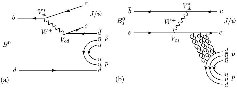
Figure 1: Leading Feynman diagrams for (a) ${{B}^{0}}\rightarrow{{J\mskip-3.0mu/\mskip-2.0mu\psi\mskip 2.0mu}}{p}\kern 1.00006pt\overline{\kern-1.00006ptp}{}$ and (b) ${{B}^{0}_{s}}\rightarrow{{J\mskip-3.0mu/\mskip-2.0mu\psi\mskip 2.0mu}}{p}\kern 1.00006pt\overline{\kern-1.00006ptp}{}$ decays.

In this Letter, the first observation of these modes along with their branching fraction and ${B}^{0}$ and ${B}^{0}_{s}$ mass measurements are reported employing a data sample corresponding to 5.2$\text{\,fb}^{-1}$ of $pp$ collision data collected by the LHCb experiment. As a normalization mode, the copious ${{B}^{0}_{s}}\rightarrow{{J\mskip-3.0mu/\mskip-2.0mu\psi\mskip 2.0mu}}\phi(\rightarrow{{K}^{+}}{{K}^{-}})$ sample is used, which is similar in topology to the signal channels.

The LHCb detector [12, 13] is a single-arm forward spectrometer covering the pseudorapidity range $2<\eta<5$, designed for the study of particles containing $b$ or $c$ quarks. The detector includes a high-precision tracking system consisting of a silicon-strip vertex detector surrounding the $pp$ interaction region [14], a large-area silicon-strip detector located upstream of a dipole magnet with a bending power of about 4 Tm, and three stations of silicon-strip detectors and straw drift tubes [15] placed downstream of the magnet. The tracking system provides a measurement of the momentum, $p$, of charged particles with a relative uncertainty that varies from 0.5% at low momentum to 1.0% at 200 GeV. Different types of charged hadrons are distinguished using information from two ring-imaging Cherenkov detectors [16]. Muons are identified by a system composed of alternating layers of iron and multiwire proportional chambers [17]. The online event selection is performed by a trigger [18], comprising a hardware stage based on information from the muon system, followed by a software stage that applies a full event reconstruction. The software trigger is a combination of event categories mostly relying on identifying ${J\mskip-3.0mu/\mskip-2.0mu\psi\mskip 2.0mu}$ decays consistent with a $B$-meson decay topology with two muon tracks originating from a secondary decay vertex detached from the primary $pp$ collision point.

The $pp$ collision data used in this analysis were collected at center-of-mass energies of 7 and 8 TeV ($3$$\text{\,fb}^{-1}$) and 13 TeV ($2.2$$\text{\,fb}^{-1}$), during the Run 1 (2011 and 2012) and Run 2 (2015 and 2016) run periods, respectively. The data taking conditions differ enough between the two run periods, such that they are analyzed separately and the results combined at the end.

Samples of simulated events are used to study the properties of the signal and control channels. The $pp$ collisions are generated using Pythia [19, *Sjostrand:2007gs] with a specific LHCb configuration [21]. Decays of hadronic particles are described by EvtGen [22], in which final-state radiation is generated using Photos [23]. For the ${{B}^{0}_{s}}\rightarrow{{J\mskip-3.0mu/\mskip-2.0mu\psi\mskip 2.0mu}}\phi$ mode, simulation samples are generated according to a decay model based on results reported in Ref. [24], while the ${B}^{0}_{\scaleto{(}{6.6pt}s\scaleto{)}{6.6pt}}\rightarrow{{J\mskip-3.0mu/\mskip-2.0mu\psi\mskip 2.0mu}}{p}\kern 1.00006pt\overline{\kern-1.00006ptp}{}$ signal modes are generated uniformly in phase space. The interactions of the generated particles with the detector and its response are implemented using the Geant4 toolkit [25, *Agostinelli:2002hh] as described in Ref. [27].

The event selection relies on the excellent vertexing and charged particle identification (PID) capabilities of the LHCb detector. For a given particle, the associated primary vertex (PV) corresponds to that with the smallest $\chi^{2}_{\rm IP}$, defined as the difference in $\chi^{2}$ between the PV fit including and excluding the particle. Signal candidates are formed starting with a pair of charged tracks, consistent with muons originating from a common vertex significantly displaced from its associated PV and with an invariant mass consistent with the ${J\mskip-3.0mu/\mskip-2.0mu\psi\mskip 2.0mu}$ meson. Another pair of oppositely charged tracks, identified as protons and originating from a common vertex, is combined with the ${J\mskip-3.0mu/\mskip-2.0mu\psi\mskip 2.0mu}$ candidate to form a ${B}^{0}_{\scaleto{(}{6.6pt}s\scaleto{)}{6.6pt}}$ candidate. The entire decay topology is submitted to a kinematic fit where the dimuon invariant mass is constrained to the known ${J\mskip-3.0mu/\mskip-2.0mu\psi\mskip 2.0mu}$ mass [28]. The ${{B}^{0}_{s}}\rightarrow{{J\mskip-3.0mu/\mskip-2.0mu\psi\mskip 2.0mu}}\phi$ control mode candidates are reconstructed in a similar fashion, replacing the ${p}\kern 1.00006pt\overline{\kern-1.00006ptp}{}$ combination with a pair of charged tracks identified as ${{K}^{+}}{{K}^{-}}$ candidates, required to have an invariant mass within $\pm 5\text{\,Me\kern-1.00006ptV}$ of the known $\phi$-meson mass [28]. All charged tracks are required to be of good quality and have $p_{\mathrm{T}}$ $>$ 300  MeV ($p_{\mathrm{T}}$ $>$ 550  MeV) for $p$ or $K$ ($\mu$). For the ${{B}^{0}_{s}}\rightarrow{{J\mskip-3.0mu/\mskip-2.0mu\psi\mskip 2.0mu}}\phi$ mode, the contamination from $B^{0}\rightarrow{{J\mskip-3.0mu/\mskip-2.0mu\psi\mskip 2.0mu}}K^{+}\pi^{-}$ decays with a pion misidentified as a kaon is rejected by imposing a ${B}^{0}$ mass veto and using PID information. At this stage, the combinatorial background dominates, comprising a correctly reconstructed ${J\mskip-3.0mu/\mskip-2.0mu\psi\mskip 2.0mu}$ meson candidate combined with two unrelated charged tracks.

At this stage, a multidimensional gradient-boosting algorithm [29] is used to weight the simulated ${{B}^{0}_{s}}\rightarrow{{J\mskip-3.0mu/\mskip-2.0mu\psi\mskip 2.0mu}}\phi$ events to match background-subtracted data distributions in all the training variables. These weights are denoted as GB-weights. The background-subtracted data distributions are obtained using the sPlot technique [30]. Under the assumption that the relative corrections between data and simulation are similar among different $B^{0}_{(s)}\rightarrow{{J\mskip-3.0mu/\mskip-2.0mu\psi\mskip 2.0mu}}h^{+}h^{\prime-}$ decay topologies, $h^{+}$ and $h^{\prime-}$ being charged hadrons, the GB-weights obtained from the control mode are applied to the signal mode. To validate this assumption, similar GB-weights are derived using another control mode, $B^{0}\rightarrow{{J\mskip-3.0mu/\mskip-2.0mu\psi\mskip 2.0mu}}{{K}^{+}}{{\pi}^{-}}$, yielding similar results.

For further background suppression, two multivariate classifiers are applied, each employing a gradient-boosted decision tree (BDT) [31]. In the first stage, the BDT_kin classifier, based on kinematical and topological variables of the ${B}^{0}_{s}$ candidate, is trained using the ${{B}^{0}_{s}}\rightarrow{{J\mskip-3.0mu/\mskip-2.0mu\psi\mskip 2.0mu}}\phi$ decays from simulation as signal proxy, and selected ${{J\mskip-3.0mu/\mskip-2.0mu\psi\mskip 2.0mu}}{{K}^{+}}{{K}^{-}}$ candidates in the mass window $[5450,5700]$ MeV as background. For BDT_kin, only kinematic variables whose distributions are similar between the signal and the control mode are employed. These include the $p$, $p_{\mathrm{T}}$, and $\chi^{2}_{\rm IP}$ values of the ${{B}^{0}_{s}}$ meson, the $\chi^{2}$ probability from a kinematic fit [32] to the decay topology, and the impact parameter (IP) of the muons with respect to the associated PV.

To choose the BDT_kin selection cut, the ${{B}^{0}_{s}}\rightarrow{{J\mskip-3.0mu/\mskip-2.0mu\psi\mskip 2.0mu}}{p}\kern 1.00006pt\overline{\kern-1.00006ptp}{}$ signal figure of merit, $S/\sqrt{S+B}$, is required to exceed five in a 2$\sigma$ window around the ${B}^{0}_{s}$ mass peak. The background yield, $B$, is estimated from a fit to the ${{J\mskip-3.0mu/\mskip-2.0mu\psi\mskip 2.0mu}}{p}\kern 1.00006pt\overline{\kern-1.00006ptp}{}$ invariant mass distribution. To estimate the expected signal yield, $S$, the central value of the ${{B}^{0}_{s}}\rightarrow{{J\mskip-3.0mu/\mskip-2.0mu\psi\mskip 2.0mu}}{p}\kern 1.00006pt\overline{\kern-1.00006ptp}{}$ branching fraction quoted in Ref. [11] is used, along with the signal efficiency obtained from simulation.

In the final selection stage, a second classifier, BDT_PID, uses the hadron PID information from the Cherenkov detector system to distinguish between pions, kaons and protons. Aside from PID, the BDT_PID training variables also include the $p$, $p_{\mathrm{T}}$ and $\chi^{2}_{\rm IP}$ values of the protons. The signal sample is taken as the ${{B}^{0}_{s}}\rightarrow{{J\mskip-3.0mu/\mskip-2.0mu\psi\mskip 2.0mu}}{p}\kern 1.00006pt\overline{\kern-1.00006ptp}{}$ simulation incorporating the GB-weights for the kinematic variables, while the background sample is taken from events in data with $m({{J\mskip-3.0mu/\mskip-2.0mu\psi\mskip 2.0mu}}p\bar{p})\in[5450,5500]$ MeV. The hadron PID variables in the simulation require further corrections to be representative of data. The PID variables are obtained from high-yield calibration samples of ${{\mathchar 28931\relax}^{+}_{c}}\rightarrow{p}{{K}^{-}}{{\pi}^{+}}$ and $D^{\ast+}\rightarrow D^{0}(\rightarrow K^{-}{{\pi}^{+}})\pi^{+}$ decays, which can be selected as a function of the $p$, $p_{\mathrm{T}}$ and the number of tracks in the event using only kinematic information [33]. The optimal BDT_PID selection criterion is chosen by maximizing the figure of merit $S/\sqrt{S+B}$, with the initial signal and background yields obtained from a fit to the $m({{J\mskip-3.0mu/\mskip-2.0mu\psi\mskip 2.0mu}}{p}\kern 1.00006pt\overline{\kern-1.00006ptp}{})$ distribution after the BDT_kin selection.

For the ${{B}^{0}_{s}}\rightarrow{{J\mskip-3.0mu/\mskip-2.0mu\psi\mskip 2.0mu}}\phi$ control mode, the selection is performed using a dedicated classifier, BDT_CS, which includes the kinematic variables considered in BDT_kin with the addition of the PID information.

After application of all selection requirements, the background is predominantly combinatorial. Approximately 1% of the selected events contain more than one candidate at this stage; a single candidate is selected randomly. The efficiency of the trigger, detector acceptance, reconstruction and selection procedure is approximately 1%, as estimated from simulation.

The ${B}^{0}$ and ${B}^{0}_{s}$ signal and background yields are determined via an extended maximum likelihood fit to the ${{J\mskip-3.0mu/\mskip-2.0mu\psi\mskip 2.0mu}}{p}\kern 1.00006pt\overline{\kern-1.00006ptp}{}$ invariant mass distribution in the range $[5220,\;5420]$ MeV. Each signal shape is modeled as the sum of two Crystal Ball [34] functions sharing a common peak position, with tails on either sides of the peak to describe the radiative and misreconstruction effects. The background shape is modeled by a first-order polynomial with parameters determined from the fit to data. The signal-model parameters are determined from simulation and only the ${B}^{0}$ and ${B}^{0}_{s}$ central mass values are left as free parameters in the fit to data. The detector invariant-mass resolution is in agreement with simulations within a factor of $1.007\pm 0.004$ as determined with the control mode. Residual discrepancies are accounted for in the systematic uncertainties. In order to validate the fit model, 1000 mass spectra are generated according to the model and fitted employing an alternative model comprising three Gaussian components for the signal and an exponential function for background. The difference between the input value of the yields and the mean of the fitted yields from the alternative model is assigned as a systematic uncertainty. The mass fit for the control mode uses a similar ${B}^{0}_{s}$ signal lineshape, with the background modeled by an exponential function. The result of the fit to the combined Run 1 and Run 2 control mode yields a signal of $136{,}800\pm 400$. The corresponding fit to the signal-mode candidates is shown in Fig. 2 with the results reported in Table 1, where clear signals of ${B}^{0}$ and ${B}^{0}_{s}$ are observed.

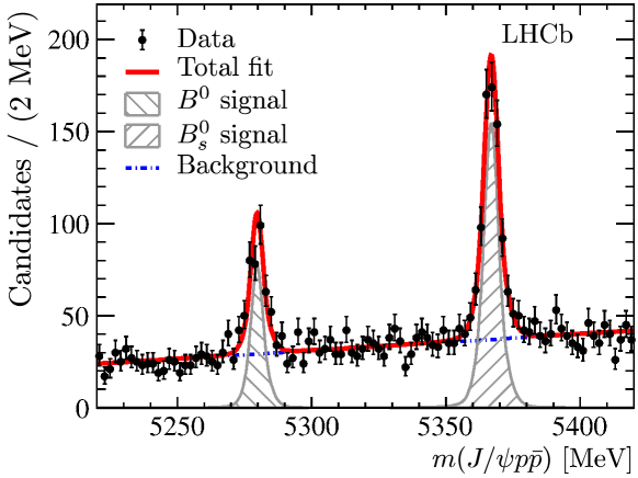
Figure 2: Fit to the ${{J\mskip-3.0mu/\mskip-2.0mu\psi\mskip 2.0mu}}{p}\kern 1.00006pt\overline{\kern-1.00006ptp}{}$ invariant-mass distribution of the ${B}^{0}_{\scaleto{(}{6.6pt}s\scaleto{)}{6.6pt}}$ signal modes.

Table 1: Signal yields and masses for ${B}^{0}$ and ${B}^{0}_{s}$ mesons.

Mode	Yield	${B}^{0}_{\scaleto{(}{6.6pt}s\scaleto{)}{6.6pt}}$ mass [MeV]
${{B}^{0}}\rightarrow{{J\mskip-3.0mu/\mskip-2.0mu\psi\mskip 2.0mu}}{p}\kern 1.00006pt\overline{\kern-1.00006ptp}{}$	$256\pm 22$	$5279.74\pm 0.30$
${{B}^{0}_{s}}\rightarrow{{J\mskip-3.0mu/\mskip-2.0mu\psi\mskip 2.0mu}}{p}\kern 1.00006pt\overline{\kern-1.00006ptp}{}$	$609\pm 31$	$5366.85\pm 0.19$

The branching fractions measured with respect to the ${{{B}^{0}_{s}}\rightarrow{{J\mskip-3.0mu/\mskip-2.0mu\psi\mskip 2.0mu}}\phi}$ control mode are

$$\frac{\mathcal{B}({{B}^{0}}\rightarrow{{J\mskip-3.0mu/\mskip-2.0mu\psi\mskip 2.0mu}}{p}\kern 1.00006pt\overline{\kern-1.00006ptp}{})}{\mathcal{B}({{B}^{0}_{s}}\rightarrow{{J\mskip-3.0mu/\mskip-2.0mu\psi\mskip 2.0mu}}\phi)\times\mathcal{B}(\phi\rightarrow{{K}^{+}}{{K}^{-}})\times f_{s}/f_{d}} =\;\frac{N^{\rm corr}_{{{B}^{0}}\rightarrow{{J\mskip-3.0mu/\mskip-2.0mu\psi\mskip 2.0mu}}{p}\kern 0.70004pt\overline{\kern-0.70004ptp}{}}}{N^{\rm corr}_{{{B}^{0}_{s}}\rightarrow{{J\mskip-3.0mu/\mskip-2.0mu\psi\mskip 2.0mu}}{{K}^{+}}{{K}^{-}}}},$$

$$\frac{\mathcal{B}({{B}^{0}_{s}}\rightarrow{{J\mskip-3.0mu/\mskip-2.0mu\psi\mskip 2.0mu}}{p}\kern 1.00006pt\overline{\kern-1.00006ptp}{})}{\mathcal{B}({{B}^{0}_{s}}\rightarrow{{J\mskip-3.0mu/\mskip-2.0mu\psi\mskip 2.0mu}}\phi)\times\mathcal{B}(\phi\rightarrow{{K}^{+}}{{K}^{-}})} =\;\frac{N^{\rm corr}_{{{B}^{0}_{s}}\rightarrow{{J\mskip-3.0mu/\mskip-2.0mu\psi\mskip 2.0mu}}{p}\kern 0.70004pt\overline{\kern-0.70004ptp}{}}}{N^{\rm corr}_{{{B}^{0}_{s}}\rightarrow{{J\mskip-3.0mu/\mskip-2.0mu\psi\mskip 2.0mu}}{{K}^{+}}{{K}^{-}}}},$$

where $f_{s}/f_{d}$ is the ratio of the $b$-quark hadronization probabilities into ${{B}^{0}_{s}}$ and ${{B}^{0}}$ mesons, and $N^{\rm corr}$ denotes efficiency-corrected signal yields. For the signal modes, since the physics model is not known a priori, an event-by-event efficiency correction is applied to the data. It is derived from simulation as a function of the kinematic variables, which are given in detail in the Appendix.

Since the control mode has a topology very similar to that of the signal mode, most of the systematic uncertainties cancel in the branching-fraction ratio measurement. Residual systematic effects of the PID efficiency estimation are due to the correction procedure. An alternative PID correction is considered using proton calibration samples from decays of the long-lived ${\mathchar 28931\relax}$ baryon to a proton and a pion, instead of prompt ${{\mathchar 28931\relax}^{+}_{c}}$ decays. The difference between the two methods is assigned as a systematic uncertainty. The degree to which the simulation describes hadronic interactions with the detector material is less accurate for baryons than it is for mesons [22]. Following Ref. [35], a systematic uncertainty of 4% (1.1%) per proton (kaon) is assigned. Other systematic effects include the choice of the fit model, the weighting procedure, the trigger efficiency, and the presence of events with more than one candidate. The overall systematic uncertainties on the ratio of branching fractions are $7.2\%$ ($7.2\%$) and $6.5\%$ ($6.6\%$) for ${B}^{0}_{s}$ (${B}^{0}$) meson in Run 1 and Run 2, respectively, where the relevant contributions, listed in Table 2, are added in quadrature. Since the detector and the analysis methods remain the same between the two run periods, the systematic uncertainties are fully correlated while the statistical uncertainties are uncorrelated. The combination of the measurements is taken as a weighted mean to give the branching fraction ratios

$$\frac{\mathcal{B}({{B}^{0}}\rightarrow{{J\mskip-3.0mu/\mskip-2.0mu\psi\mskip 2.0mu}}{p}\kern 1.00006pt\overline{\kern-1.00006ptp}{})}{\mathcal{B}({{B}^{0}_{s}}\rightarrow{{J\mskip-3.0mu/\mskip-2.0mu\psi\mskip 2.0mu}}\phi)\times\mathcal{B}(\phi\rightarrow{{K}^{+}}{{K}^{-}})\times f_{s}/f_{d}} =(0.329\pm 0.029\;(\text{stat})\pm 0.022\;(\text{syst}))\times 10^{-2},$$

$$\frac{\mathcal{B}({{B}^{0}_{s}}\rightarrow{{J\mskip-3.0mu/\mskip-2.0mu\psi\mskip 2.0mu}}{p}\kern 1.00006pt\overline{\kern-1.00006ptp}{})}{\mathcal{B}({{B}^{0}_{s}}\rightarrow{{J\mskip-3.0mu/\mskip-2.0mu\psi\mskip 2.0mu}}\phi)\times\mathcal{B}(\phi\rightarrow{{K}^{+}}{{K}^{-}})} =(0.706\pm 0.037\;(\text{stat})\pm 0.048\;(\text{syst}))\times 10^{-2},$$

where the first uncertainty is statistical and the second is systematic. For the absolute branching-fraction determination, the value ${\mathcal{B}({{B}^{0}_{s}}\rightarrow{{J\mskip-3.0mu/\mskip-2.0mu\psi\mskip 2.0mu}}\phi)\times\mathcal{B}(\phi\rightarrow{{K}^{+}}{{K}^{-}})\times f_{s}/f_{d}=(1.314\pm 0.016\pm 0.079)\times 10^{-4}}$ is obtained from Ref. [36] as the product of the two branching ratios, ${\mathcal{B}({{B}^{0}_{s}}\rightarrow{{J\mskip-3.0mu/\mskip-2.0mu\psi\mskip 2.0mu}}\phi)=(10.50\pm 0.13\pm 0.64)\times 10^{-4}}$ and $\mathcal{B}(\phi\rightarrow{{K}^{+}}{{K}^{-}})=0.489\pm 0.005$, and the ratio of fragmentation probabilities ${f_{s}/f_{d}=0.256\pm 0.020}$ [37]. For the ${B}^{0}_{s}$-meson normalization, the updated ratio ${f_{s}/f_{d}=0.259\pm 0.015}$ [37] is used in Run 1, while for Run 2 it has been multiplied by an additional scale factor of $1.068\pm 0.046$ [38] to take into account the dependence on the center of mass energy. The small $S$-wave $K^{+}K^{-}$ fraction under the $\phi(1020)$ resonance, $F_{S}=0.0070\pm 0.0005$ [36], is accounted for as a correction. The absolute branching fractions are then combined to give

$$\mathcal{B}({{B}^{0}}\rightarrow{{J\mskip-3.0mu/\mskip-2.0mu\psi\mskip 2.0mu}}{p}\kern 1.00006pt\overline{\kern-1.00006ptp}{}) =(4.51\pm 0.40\;\text{(stat)}\pm 0.44\;\text{(syst)})\times 10^{-7},$$

$$\mathcal{B}({{B}^{0}_{s}}\rightarrow{{J\mskip-3.0mu/\mskip-2.0mu\psi\mskip 2.0mu}}{p}\kern 1.00006pt\overline{\kern-1.00006ptp}{}) =(3.58\pm 0.19\;\text{(stat)}\pm 0.39\;\text{(syst)})\times 10^{-6},$$

where the systematic uncertainty is the sum in quadrature of the overall systematic contribution on the ratio of branching fractions, the normalization mode uncertainty and the $f_{s}/f_{d}$ uncertainty for the ${B}^{0}_{s}$ signal. Table 2 summarizes the systematic uncertainties separately for the run periods. The dominant contributions are the normalization, the PID, and the tracking systematic uncertainties. For the ${B}^{0}$ meson, the external normalization measurement from Run 1, $\mathcal{B}({{B}^{0}_{s}}\rightarrow{{J\mskip-3.0mu/\mskip-2.0mu\psi\mskip 2.0mu}}\phi)\times\mathcal{B}(\phi\rightarrow{{K}^{+}}{{K}^{-}})\times f_{s}/f_{d}$ [36] is used, while for Run 2 the additional energy-dependent correction on $f_{s}/f_{d}$ has an uncertainty of 4.3%. For the ${B}^{0}_{s}$ meson, the measured $\mathcal{B}({{B}^{0}_{s}}\rightarrow{{J\mskip-3.0mu/\mskip-2.0mu\psi\mskip 2.0mu}}\phi)\times\mathcal{B}(\phi\rightarrow{{K}^{+}}{{K}^{-}})\times f_{s}/f_{d}$ is divided by $f_{s}/f_{d}$ to obtain the ${B}^{0}_{s}$ normalization, $\mathcal{B}({{B}^{0}_{s}}\rightarrow{{J\mskip-3.0mu/\mskip-2.0mu\psi\mskip 2.0mu}}\phi)\times\mathcal{B}(\phi\rightarrow{{K}^{+}}{{K}^{-}})$, resulting in an uncertainty on $f_{s}/f_{d}$ independent of the run condition.

Table 2: Systematic uncertainties on the branching fraction measurements for Run 1 and Run 2. The total uncertainties on the branching fraction ratios (${\rm BFR}$) are the sum of the systematic uncertainties, added in quadrature. The total uncertainties on the absolute branching fractions ($\mathcal{B}$) include the normalization and the uncertainties on the ratio $f_{s}/f_{d}$ from external measurments as well.

	$\mathcal{B}({{B}^{0}}\rightarrow{{J\mskip-3.0mu/\mskip-2.0mu\psi\mskip 2.0mu}}{p}\kern 1.00006pt\overline{\kern-1.00006ptp}{})$	$\mathcal{B}({{B}^{0}_{s}}\rightarrow{{J\mskip-3.0mu/\mskip-2.0mu\psi\mskip 2.0mu}}{p}\kern 1.00006pt\overline{\kern-1.00006ptp}{})$
	Run 1 (Run 2)	Run 1 (Run 2)
Fit model	1.0 (0.5)%	1.0 (0.9)%
Detector resolution	0.6 (0.5)%	0.4 (0.6)%
PID efficiency	5.0 (4.0)%	5.0 (4.0)%
Trigger	1.0 (1.0)%	1.0 (1.0)%
Tracking	5.0 (5.0)%	5.0 (5.0)%
Simulation weighting	0.4 (0.4)%	0.3 (0.3)%
Multiple candidates	0.1 (0.1)%	0.1 (0.1)%
Total on ${\rm BFR}$	7.2 (6.5)%	7.2 (6.6)%
Normalization	6.1 (6.1)%	6.1 (6.1)%
$f_{s}/f_{d}$	$\;-\;\;(4.3)\%$	5.8 (5.8)%
Total on $\mathcal{B}$	$\;\;9.4\;(10.1)$%	11.1 (10.7)%

Table 3: Systematic uncertainties of ${B}^{0}$ and ${B}^{0}_{s}$ mass measurements.

	${B}^{0}$	${B}^{0}_{s}$
	[MeV]	[MeV]
Momentum scale	0.097	0.124
Mass fit model	0.020	0.020
Energy loss correction	0.030	0.030
Total	0.103	0.129

In addition, the small $Q$-values of the ${B}^{0}_{\scaleto{(}{6.6pt}s\scaleto{)}{6.6pt}}\rightarrow{{J\mskip-3.0mu/\mskip-2.0mu\psi\mskip 2.0mu}}{p}\kern 1.00006pt\overline{\kern-1.00006ptp}{}$ decays also allow for precise measurements of the ${B}^{0}$ and ${B}^{0}_{s}$ masses, with a resolution of 3.3 MeV (3.8 MeV) for the ${B}^{0}$ (${B}^{0}_{s}$) meson. The sources of systematic uncertainties include momentum scaling due to imperfections in the magnetic-field mapping derived using well-known narrow resonances, uncertainties on particle interactions with the detector material, and the choice of the signal model, as reported in Table 3. The uncertainty on the proton mass is neglected. The final results are

$${m_{{{B}^{0}}}} =5279.74\pm 0.30\;({\rm stat})\pm 0.10\;({\rm syst})\text{\,Me\kern-1.00006ptV},$$

$${m_{{{B}^{0}_{s}}}} =5366.85\pm 0.19\;({\rm stat})\pm 0.13\;({\rm syst})\text{\,Me\kern-1.00006ptV},$$

with a correlation of $4\times 10^{-4}$ in the statistical uncertainty. These represent the most precise single measurements for the ${B}^{0}$ and ${B}^{0}_{s}$ masses.

In summary, the first observation of the ${{B}^{0}}\rightarrow{{J\mskip-3.0mu/\mskip-2.0mu\psi\mskip 2.0mu}}{p}\kern 1.00006pt\overline{\kern-1.00006ptp}{}$ and ${{B}^{0}_{s}}\rightarrow{{J\mskip-3.0mu/\mskip-2.0mu\psi\mskip 2.0mu}}{p}\kern 1.00006pt\overline{\kern-1.00006ptp}{}$ decays is reported. The measured branching fraction for the ${{B}^{0}}\rightarrow{{J\mskip-3.0mu/\mskip-2.0mu\psi\mskip 2.0mu}}{p}\kern 1.00006pt\overline{\kern-1.00006ptp}{}$ decay is consistent with theoretical expectations [10] while that for ${{B}^{0}_{s}}\rightarrow{{J\mskip-3.0mu/\mskip-2.0mu\psi\mskip 2.0mu}}{p}\kern 1.00006pt\overline{\kern-1.00006ptp}{}$ is enhanced by two orders of magnitude with respect to predictions without resonant contributions [10]. More data are needed for glueball and pentaquark searches through a full Dalitz plot analysis. The world’s best single measurements of the ${B}^{0}$ and ${B}^{0}_{s}$ masses are also reported.

LHCb Collaboration

R. Aaij²⁹, C. Abellán Beteta⁴⁶, B. Adeva⁴³, M. Adinolfi⁵⁰, C.A. Aidala⁷⁷, Z. Ajaltouni⁷, S. Akar⁶¹, P. Albicocco²⁰, J. Albrecht¹², F. Alessio⁴⁴, M. Alexander⁵⁵, A. Alfonso Albero⁴², G. Alkhazov³⁵, P. Alvarez Cartelle⁵⁷, A.A. Alves Jr⁴³, S. Amato², S. Amerio²⁵, Y. Amhis⁹, L. An¹⁹, L. Anderlini¹⁹, G. Andreassi⁴⁵, M. Andreotti¹⁸, J.E. Andrews⁶², F. Archilli²⁹, J. Arnau Romeu⁸, A. Artamonov⁴¹, M. Artuso⁶³, K. Arzymatov³⁹, E. Aslanides⁸, M. Atzeni⁴⁶, B. Audurier²⁴, S. Bachmann¹⁴, J.J. Back⁵², S. Baker⁵⁷, V. Balagura^9,b, W. Baldini¹⁸, A. Baranov³⁹, R.J. Barlow⁵⁸, G.C. Barrand⁹, S. Barsuk⁹, W. Barter⁵⁸, M. Bartolini²¹, F. Baryshnikov⁷³, V. Batozskaya³³, B. Batsukh⁶³, A. Battig¹², V. Battista⁴⁵, A. Bay⁴⁵, J. Beddow⁵⁵, F. Bedeschi²⁶, I. Bediaga¹, A. Beiter⁶³, L.J. Bel²⁹, S. Belin²⁴, N. Beliy⁴, V. Bellee⁴⁵, N. Belloli^22,i, K. Belous⁴¹, I. Belyaev³⁶, G. Bencivenni²⁰, E. Ben-Haim¹⁰, S. Benson²⁹, S. Beranek¹¹, A. Berezhnoy³⁷, R. Bernet⁴⁶, D. Berninghoff¹⁴, E. Bertholet¹⁰, A. Bertolin²⁵, C. Betancourt⁴⁶, F. Betti^17,44, M.O. Bettler⁵¹, Ia. Bezshyiko⁴⁶, S. Bhasin⁵⁰, J. Bhom³¹, M.S. Bieker¹², S. Bifani⁴⁹, P. Billoir¹⁰, A. Birnkraut¹², A. Bizzeti^19,u, M. Bjørn⁵⁹, M.P. Blago⁴⁴, T. Blake⁵², F. Blanc⁴⁵, S. Blusk⁶³, D. Bobulska⁵⁵, V. Bocci²⁸, O. Boente Garcia⁴³, T. Boettcher⁶⁰, A. Bondar^40,x, N. Bondar³⁵, S. Borghi^58,44, M. Borisyak³⁹, M. Borsato⁴³, M. Boubdir¹¹, T.J.V. Bowcock⁵⁶, C. Bozzi^18,44, S. Braun¹⁴, M. Brodski⁴⁴, J. Brodzicka³¹, A. Brossa Gonzalo⁵², D. Brundu^24,44, E. Buchanan⁵⁰, A. Buonaura⁴⁶, C. Burr⁵⁸, A. Bursche²⁴, J. Buytaert⁴⁴, W. Byczynski⁴⁴, S. Cadeddu²⁴, H. Cai⁶⁷, R. Calabrese^18,g, R. Calladine⁴⁹, M. Calvi^22,i, M. Calvo Gomez^42,m, A. Camboni^42,m, P. Campana²⁰, D.H. Campora Perez⁴⁴, L. Capriotti^17,e, A. Carbone^17,e, G. Carboni²⁷, R. Cardinale²¹, A. Cardini²⁴, P. Carniti^22,i, K. Carvalho Akiba², G. Casse⁵⁶, M. Cattaneo⁴⁴, G. Cavallero²¹, R. Cenci^26,p, D. Chamont⁹, M.G. Chapman⁵⁰, M. Charles¹⁰, Ph. Charpentier⁴⁴, G. Chatzikonstantinidis⁴⁹, M. Chefdeville⁶, V. Chekalina³⁹, C. Chen³, S. Chen²⁴, S.-G. Chitic⁴⁴, V. Chobanova⁴³, M. Chrzaszcz⁴⁴, A. Chubykin³⁵, P. Ciambrone²⁰, X. Cid Vidal⁴³, G. Ciezarek⁴⁴, F. Cindolo¹⁷, P.E.L. Clarke⁵⁴, M. Clemencic⁴⁴, H.V. Cliff⁵¹, J. Closier⁴⁴, V. Coco⁴⁴, J.A.B. Coelho⁹, J. Cogan⁸, E. Cogneras⁷, L. Cojocariu³⁴, P. Collins⁴⁴, T. Colombo⁴⁴, A. Comerma-Montells¹⁴, A. Contu²⁴, G. Coombs⁴⁴, S. Coquereau⁴², G. Corti⁴⁴, M. Corvo^18,g, C.M. Costa Sobral⁵², B. Couturier⁴⁴, G.A. Cowan⁵⁴, D.C. Craik⁶⁰, A. Crocombe⁵², M. Cruz Torres¹, R. Currie⁵⁴, F. Da Cunha Marinho², C.L. Da Silva⁷⁸, E. Dall’Occo²⁹, J. Dalseno^43,v, C. D’Ambrosio⁴⁴, A. Danilina³⁶, P. d’Argent¹⁴, A. Davis⁵⁸, O. De Aguiar Francisco⁴⁴, K. De Bruyn⁴⁴, S. De Capua⁵⁸, M. De Cian⁴⁵, J.M. De Miranda¹, L. De Paula², M. De Serio^16,d, P. De Simone²⁰, J.A. de Vries²⁹, C.T. Dean⁵⁵, W. Dean⁷⁷, D. Decamp⁶, L. Del Buono¹⁰, B. Delaney⁵¹, H.-P. Dembinski¹³, M. Demmer¹², A. Dendek³², D. Derkach⁷⁴, O. Deschamps⁷, F. Desse⁹, F. Dettori⁵⁶, B. Dey⁶⁸, A. Di Canto⁴⁴, P. Di Nezza²⁰, S. Didenko⁷³, H. Dijkstra⁴⁴, F. Dordei²⁴, M. Dorigo^44,y, A.C. dos Reis¹, A. Dosil Suárez⁴³, L. Douglas⁵⁵, A. Dovbnya⁴⁷, K. Dreimanis⁵⁶, L. Dufour²⁹, G. Dujany¹⁰, P. Durante⁴⁴, J.M. Durham⁷⁸, D. Dutta⁵⁸, R. Dzhelyadin^41,†, M. Dziewiecki¹⁴, A. Dziurda³¹, A. Dzyuba³⁵, S. Easo⁵³, U. Egede⁵⁷, V. Egorychev³⁶, S. Eidelman^40,x, S. Eisenhardt⁵⁴, U. Eitschberger¹², R. Ekelhof¹², L. Eklund⁵⁵, S. Ely⁶³, A. Ene³⁴, S. Escher¹¹, S. Esen²⁹, T. Evans⁶¹, A. Falabella¹⁷, C. Färber⁴⁴, N. Farley⁴⁹, S. Farry⁵⁶, D. Fazzini^22,44,i, M. Féo⁴⁴, P. Fernandez Declara⁴⁴, A. Fernandez Prieto⁴³, F. Ferrari^17,e, L. Ferreira Lopes⁴⁵, F. Ferreira Rodrigues², M. Ferro-Luzzi⁴⁴, S. Filippov³⁸, R.A. Fini¹⁶, M. Fiorini^18,g, M. Firlej³², C. Fitzpatrick⁴⁵, T. Fiutowski³², F. Fleuret^9,b, M. Fontana⁴⁴, F. Fontanelli^21,h, R. Forty⁴⁴, V. Franco Lima⁵⁶, M. Frank⁴⁴, C. Frei⁴⁴, J. Fu^23,q, W. Funk⁴⁴, E. Gabriel⁵⁴, A. Gallas Torreira⁴³, D. Galli^17,e, S. Gallorini²⁵, S. Gambetta⁵⁴, Y. Gan³, M. Gandelman², P. Gandini²³, Y. Gao³, L.M. Garcia Martin⁷⁶, J. García Pardiñas⁴⁶, B. Garcia Plana⁴³, J. Garra Tico⁵¹, L. Garrido⁴², D. Gascon⁴², C. Gaspar⁴⁴, L. Gavardi¹², G. Gazzoni⁷, D. Gerick¹⁴, E. Gersabeck⁵⁸, M. Gersabeck⁵⁸, T. Gershon⁵², D. Gerstel⁸, Ph. Ghez⁶, V. Gibson⁵¹, O.G. Girard⁴⁵, P. Gironella Gironell⁴², L. Giubega³⁴, K. Gizdov⁵⁴, V.V. Gligorov¹⁰, C. Göbel⁶⁵, D. Golubkov³⁶, A. Golutvin^57,73, A. Gomes^1,a, I.V. Gorelov³⁷, C. Gotti^22,i, E. Govorkova²⁹, J.P. Grabowski¹⁴, R. Graciani Diaz⁴², L.A. Granado Cardoso⁴⁴, E. Graugés⁴², E. Graverini⁴⁶, G. Graziani¹⁹, A. Grecu³⁴, R. Greim²⁹, P. Griffith²⁴, L. Grillo⁵⁸, L. Gruber⁴⁴, B.R. Gruberg Cazon⁵⁹, O. Grünberg⁷⁰, C. Gu³, E. Gushchin³⁸, A. Guth¹¹, Yu. Guz^41,44, T. Gys⁴⁴, T. Hadavizadeh⁵⁹, C. Hadjivasiliou⁷, G. Haefeli⁴⁵, C. Haen⁴⁴, S.C. Haines⁵¹, B. Hamilton⁶², X. Han¹⁴, T.H. Hancock⁵⁹, S. Hansmann-Menzemer¹⁴, N. Harnew⁵⁹, T. Harrison⁵⁶, C. Hasse⁴⁴, M. Hatch⁴⁴, J. He⁴, M. Hecker⁵⁷, K. Heinicke¹², A. Heister¹², K. Hennessy⁵⁶, L. Henry⁷⁶, M. Heß⁷⁰, J. Heuel¹¹, A. Hicheur⁶⁴, R. Hidalgo Charman⁵⁸, D. Hill⁵⁹, M. Hilton⁵⁸, P.H. Hopchev⁴⁵, J. Hu¹⁴, W. Hu⁶⁸, W. Huang⁴, Z.C. Huard⁶¹, W. Hulsbergen²⁹, T. Humair⁵⁷, M. Hushchyn⁷⁴, D. Hutchcroft⁵⁶, D. Hynds²⁹, P. Ibis¹², M. Idzik³², P. Ilten⁴⁹, A. Inglessi³⁵, A. Inyakin⁴¹, K. Ivshin³⁵, R. Jacobsson⁴⁴, J. Jalocha⁵⁹, E. Jans²⁹, B.K. Jashal⁷⁶, A. Jawahery⁶², F. Jiang³, M. John⁵⁹, D. Johnson⁴⁴, C.R. Jones⁵¹, C. Joram⁴⁴, B. Jost⁴⁴, N. Jurik⁵⁹, S. Kandybei⁴⁷, M. Karacson⁴⁴, J.M. Kariuki⁵⁰, S. Karodia⁵⁵, N. Kazeev⁷⁴, M. Kecke¹⁴, F. Keizer⁵¹, M. Kelsey⁶³, M. Kenzie⁵¹, T. Ketel³⁰, E. Khairullin³⁹, B. Khanji⁴⁴, C. Khurewathanakul⁴⁵, K.E. Kim⁶³, T. Kirn¹¹, V.S. Kirsebom⁴⁵, S. Klaver²⁰, K. Klimaszewski³³, T. Klimkovich¹³, S. Koliiev⁴⁸, M. Kolpin¹⁴, R. Kopecna¹⁴, P. Koppenburg²⁹, I. Kostiuk^29,48, S. Kotriakhova³⁵, M. Kozeiha⁷, L. Kravchuk³⁸, M. Kreps⁵², F. Kress⁵⁷, P. Krokovny^40,x, W. Krupa³², W. Krzemien³³, W. Kucewicz^31,l, M. Kucharczyk³¹, V. Kudryavtsev^40,x, A.K. Kuonen⁴⁵, T. Kvaratskheliya^36,44, D. Lacarrere⁴⁴, G. Lafferty⁵⁸, A. Lai²⁴, D. Lancierini⁴⁶, G. Lanfranchi²⁰, C. Langenbruch¹¹, T. Latham⁵², C. Lazzeroni⁴⁹, R. Le Gac⁸, R. Lefèvre⁷, A. Leflat³⁷, F. Lemaitre⁴⁴, O. Leroy⁸, T. Lesiak³¹, B. Leverington¹⁴, P.-R. Li^4,ab, Y. Li⁵, Z. Li⁶³, X. Liang⁶³, T. Likhomanenko⁷², R. Lindner⁴⁴, F. Lionetto⁴⁶, V. Lisovskyi⁹, G. Liu⁶⁶, X. Liu³, D. Loh⁵², A. Loi²⁴, I. Longstaff⁵⁵, J.H. Lopes², G.H. Lovell⁵¹, D. Lucchesi^25,o, M. Lucio Martinez⁴³, Y. Luo³, A. Lupato²⁵, E. Luppi^18,g, O. Lupton⁴⁴, A. Lusiani²⁶, X. Lyu⁴, F. Machefert⁹, F. Maciuc³⁴, V. Macko⁴⁵, P. Mackowiak¹², S. Maddrell-Mander⁵⁰, O. Maev^35,44, K. Maguire⁵⁸, D. Maisuzenko³⁵, M.W. Majewski³², S. Malde⁵⁹, B. Malecki⁴⁴, A. Malinin⁷², T. Maltsev^40,x, H. Malygina¹⁴, G. Manca^24,f, G. Mancinelli⁸, D. Marangotto^23,q, J. Maratas^7,w, J.F. Marchand⁶, U. Marconi¹⁷, C. Marin Benito⁹, M. Marinangeli⁴⁵, P. Marino⁴⁵, J. Marks¹⁴, P.J. Marshall⁵⁶, G. Martellotti²⁸, M. Martinelli⁴⁴, D. Martinez Santos⁴³, F. Martinez Vidal⁷⁶, A. Massafferri¹, M. Materok¹¹, R. Matev⁴⁴, A. Mathad⁵², Z. Mathe⁴⁴, C. Matteuzzi²², A. Mauri⁴⁶, E. Maurice^9,b, B. Maurin⁴⁵, M. McCann^57,44, A. McNab⁵⁸, R. McNulty¹⁵, J.V. Mead⁵⁶, B. Meadows⁶¹, C. Meaux⁸, N. Meinert⁷⁰, D. Melnychuk³³, M. Merk²⁹, A. Merli^23,q, E. Michielin²⁵, D.A. Milanes⁶⁹, E. Millard⁵², M.-N. Minard⁶, L. Minzoni^18,g, D.S. Mitzel¹⁴, A. Mödden¹², A. Mogini¹⁰, R.D. Moise⁵⁷, T. Mombächer¹², I.A. Monroy⁶⁹, S. Monteil⁷, M. Morandin²⁵, G. Morello²⁰, M.J. Morello^26,t, O. Morgunova⁷², J. Moron³², A.B. Morris⁸, R. Mountain⁶³, F. Muheim⁵⁴, M. Mukherjee⁶⁸, M. Mulder²⁹, D. Müller⁴⁴, J. Müller¹², K. Müller⁴⁶, V. Müller¹², C.H. Murphy⁵⁹, D. Murray⁵⁸, P. Naik⁵⁰, T. Nakada⁴⁵, R. Nandakumar⁵³, A. Nandi⁵⁹, T. Nanut⁴⁵, I. Nasteva², M. Needham⁵⁴, N. Neri^23,q, S. Neubert¹⁴, N. Neufeld⁴⁴, R. Newcombe⁵⁷, T.D. Nguyen⁴⁵, C. Nguyen-Mau^45,n, S. Nieswand¹¹, R. Niet¹², N. Nikitin³⁷, A. Nogay⁷², N.S. Nolte⁴⁴, A. Oblakowska-Mucha³², V. Obraztsov⁴¹, S. Ogilvy⁵⁵, D.P. O’Hanlon¹⁷, R. Oldeman^24,f, C.J.G. Onderwater⁷¹, A. Ossowska³¹, J.M. Otalora Goicochea², T. Ovsiannikova³⁶, P. Owen⁴⁶, A. Oyanguren⁷⁶, P.R. Pais⁴⁵, T. Pajero^26,t, A. Palano¹⁶, M. Palutan²⁰, G. Panshin⁷⁵, A. Papanestis⁵³, M. Pappagallo⁵⁴, L.L. Pappalardo^18,g, W. Parker⁶², C. Parkes^58,44, G. Passaleva^19,44, A. Pastore¹⁶, M. Patel⁵⁷, C. Patrignani^17,e, A. Pearce⁴⁴, A. Pellegrino²⁹, G. Penso²⁸, M. Pepe Altarelli⁴⁴, S. Perazzini⁴⁴, D. Pereima³⁶, P. Perret⁷, L. Pescatore⁴⁵, K. Petridis⁵⁰, A. Petrolini^21,h, A. Petrov⁷², S. Petrucci⁵⁴, M. Petruzzo^23,q, B. Pietrzyk⁶, G. Pietrzyk⁴⁵, M. Pikies³¹, M. Pili⁵⁹, D. Pinci²⁸, J. Pinzino⁴⁴, F. Pisani⁴⁴, A. Piucci¹⁴, V. Placinta³⁴, S. Playfer⁵⁴, J. Plews⁴⁹, M. Plo Casasus⁴³, F. Polci¹⁰, M. Poli Lener²⁰, A. Poluektov⁸, N. Polukhina^73,c, I. Polyakov⁶³, E. Polycarpo², G.J. Pomery⁵⁰, S. Ponce⁴⁴, A. Popov⁴¹, D. Popov^49,13, S. Poslavskii⁴¹, E. Price⁵⁰, J. Prisciandaro⁴³, C. Prouve⁴³, V. Pugatch⁴⁸, A. Puig Navarro⁴⁶, H. Pullen⁵⁹, G. Punzi^26,p, W. Qian⁴, J. Qin⁴, R. Quagliani¹⁰, B. Quintana⁷, N.V. Raab¹⁵, B. Rachwal³², J.H. Rademacker⁵⁰, M. Rama²⁶, M. Ramos Pernas⁴³, M.S. Rangel², F. Ratnikov^39,74, G. Raven³⁰, M. Ravonel Salzgeber⁴⁴, M. Reboud⁶, F. Redi⁴⁵, S. Reichert¹², F. Reiss¹⁰, C. Remon Alepuz⁷⁶, Z. Ren³, V. Renaudin⁵⁹, S. Ricciardi⁵³, S. Richards⁵⁰, K. Rinnert⁵⁶, P. Robbe⁹, A. Robert¹⁰, A.B. Rodrigues⁴⁵, E. Rodrigues⁶¹, J.A. Rodriguez Lopez⁶⁹, M. Roehrken⁴⁴, S. Roiser⁴⁴, A. Rollings⁵⁹, V. Romanovskiy⁴¹, A. Romero Vidal⁴³, J.D. Roth⁷⁷, M. Rotondo²⁰, M.S. Rudolph⁶³, T. Ruf⁴⁴, J. Ruiz Vidal⁷⁶, J.J. Saborido Silva⁴³, N. Sagidova³⁵, B. Saitta^24,f, V. Salustino Guimaraes⁶⁵, C. Sanchez Gras²⁹, C. Sanchez Mayordomo⁷⁶, B. Sanmartin Sedes⁴³, R. Santacesaria²⁸, C. Santamarina Rios⁴³, M. Santimaria^20,44, E. Santovetti^27,j, G. Sarpis⁵⁸, A. Sarti^20,k, C. Satriano^28,s, A. Satta²⁷, M. Saur⁴, D. Savrina^36,37, S. Schael¹¹, M. Schellenberg¹², M. Schiller⁵⁵, H. Schindler⁴⁴, M. Schmelling¹³, T. Schmelzer¹², B. Schmidt⁴⁴, O. Schneider⁴⁵, A. Schopper⁴⁴, H.F. Schreiner⁶¹, M. Schubiger⁴⁵, S. Schulte⁴⁵, M.H. Schune⁹, R. Schwemmer⁴⁴, B. Sciascia²⁰, A. Sciubba^28,k, A. Semennikov³⁶, E.S. Sepulveda¹⁰, A. Sergi⁴⁹, N. Serra⁴⁶, J. Serrano⁸, L. Sestini²⁵, A. Seuthe¹², P. Seyfert⁴⁴, M. Shapkin⁴¹, Y. Shcheglov^35,†, T. Shears⁵⁶, L. Shekhtman^40,x, V. Shevchenko⁷², E. Shmanin⁷³, B.G. Siddi¹⁸, R. Silva Coutinho⁴⁶, L. Silva de Oliveira², G. Simi^25,o, S. Simone^16,d, I. Skiba¹⁸, N. Skidmore¹⁴, T. Skwarnicki⁶³, M.W. Slater⁴⁹, J.G. Smeaton⁵¹, E. Smith¹¹, I.T. Smith⁵⁴, M. Smith⁵⁷, M. Soares¹⁷, l. Soares Lavra¹, M.D. Sokoloff⁶¹, F.J.P. Soler⁵⁵, B. Souza De Paula², B. Spaan¹², E. Spadaro Norella^23,q, P. Spradlin⁵⁵, F. Stagni⁴⁴, M. Stahl¹⁴, S. Stahl⁴⁴, P. Stefko⁴⁵, S. Stefkova⁵⁷, O. Steinkamp⁴⁶, S. Stemmle¹⁴, O. Stenyakin⁴¹, M. Stepanova³⁵, H. Stevens¹², A. Stocchi⁹, S. Stone⁶³, B. Storaci⁴⁶, S. Stracka²⁶, M.E. Stramaglia⁴⁵, M. Straticiuc³⁴, U. Straumann⁴⁶, S. Strokov⁷⁵, J. Sun³, L. Sun⁶⁷, Y. Sun⁶², K. Swientek³², A. Szabelski³³, T. Szumlak³², M. Szymanski⁴, Z. Tang³, T. Tekampe¹², G. Tellarini¹⁸, F. Teubert⁴⁴, E. Thomas⁴⁴, M.J. Tilley⁵⁷, V. Tisserand⁷, S. T’Jampens⁶, M. Tobin³², S. Tolk⁴⁴, L. Tomassetti^18,g, D. Tonelli²⁶, D.Y. Tou¹⁰, R. Tourinho Jadallah Aoude¹, E. Tournefier⁶, M. Traill⁵⁵, M.T. Tran⁴⁵, A. Trisovic⁵¹, A. Tsaregorodtsev⁸, G. Tuci^26,p, A. Tully⁵¹, N. Tuning^29,44, A. Ukleja³³, A. Usachov⁹, A. Ustyuzhanin^39,74, U. Uwer¹⁴, A. Vagner⁷⁵, V. Vagnoni¹⁷, A. Valassi⁴⁴, S. Valat⁴⁴, G. Valenti¹⁷, M. van Beuzekom²⁹, E. van Herwijnen⁴⁴, J. van Tilburg²⁹, M. van Veghel²⁹, R. Vazquez Gomez⁴⁴, P. Vazquez Regueiro⁴³, C. Vázquez Sierra²⁹, S. Vecchi¹⁸, J.J. Velthuis⁵⁰, M. Veltri^19,r, G. Veneziano⁵⁹, A. Venkateswaran⁶³, M. Vernet⁷, M. Veronesi²⁹, M. Vesterinen⁵², J.V. Viana Barbosa⁴⁴, D. Vieira⁴, M. Vieites Diaz⁴³, H. Viemann⁷⁰, X. Vilasis-Cardona^42,m, A. Vitkovskiy²⁹, M. Vitti⁵¹, V. Volkov³⁷, A. Vollhardt⁴⁶, D. Vom Bruch¹⁰, B. Voneki⁴⁴, A. Vorobyev³⁵, V. Vorobyev^40,x, N. Voropaev³⁵, R. Waldi⁷⁰, J. Walsh²⁶, J. Wang⁵, M. Wang³, Y. Wang⁶⁸, Z. Wang⁴⁶, D.R. Ward⁵¹, H.M. Wark⁵⁶, N.K. Watson⁴⁹, D. Websdale⁵⁷, A. Weiden⁴⁶, C. Weisser⁶⁰, M. Whitehead¹¹, G. Wilkinson⁵⁹, M. Wilkinson⁶³, I. Williams⁵¹, M. Williams⁶⁰, M.R.J. Williams⁵⁸, T. Williams⁴⁹, F.F. Wilson⁵³, M. Winn⁹, W. Wislicki³³, M. Witek³¹, G. Wormser⁹, S.A. Wotton⁵¹, K. Wyllie⁴⁴, D. Xiao⁶⁸, Y. Xie⁶⁸, A. Xu³, M. Xu⁶⁸, Q. Xu⁴, Z. Xu⁶, Z. Xu³, Z. Yang³, Z. Yang⁶², Y. Yao⁶³, L.E. Yeomans⁵⁶, H. Yin⁶⁸, J. Yu^68,aa, X. Yuan⁶³, O. Yushchenko⁴¹, K.A. Zarebski⁴⁹, M. Zavertyaev^13,c, D. Zhang⁶⁸, L. Zhang³, W.C. Zhang^3,z, Y. Zhang⁴⁴, A. Zhelezov¹⁴, Y. Zheng⁴, X. Zhu³, V. Zhukov^11,37, J.B. Zonneveld⁵⁴, S. Zucchelli^17,e.

¹Centro Brasileiro de Pesquisas Físicas (CBPF), Rio de Janeiro, Brazil
²Universidade Federal do Rio de Janeiro (UFRJ), Rio de Janeiro, Brazil
³Center for High Energy Physics, Tsinghua University, Beijing, China
⁴University of Chinese Academy of Sciences, Beijing, China
⁵Institute Of High Energy Physics (ihep), Beijing, China
⁶Univ. Grenoble Alpes, Univ. Savoie Mont Blanc, CNRS, IN2P3-LAPP, Annecy, France
⁷Université Clermont Auvergne, CNRS/IN2P3, LPC, Clermont-Ferrand, France
⁸Aix Marseille Univ, CNRS/IN2P3, CPPM, Marseille, France
⁹LAL, Univ. Paris-Sud, CNRS/IN2P3, Université Paris-Saclay, Orsay, France
¹⁰LPNHE, Sorbonne Université, Paris Diderot Sorbonne Paris Cité, CNRS/IN2P3, Paris, France
¹¹I. Physikalisches Institut, RWTH Aachen University, Aachen, Germany
¹²Fakultät Physik, Technische Universität Dortmund, Dortmund, Germany
¹³Max-Planck-Institut für Kernphysik (MPIK), Heidelberg, Germany
¹⁴Physikalisches Institut, Ruprecht-Karls-Universität Heidelberg, Heidelberg, Germany
¹⁵School of Physics, University College Dublin, Dublin, Ireland
¹⁶INFN Sezione di Bari, Bari, Italy
¹⁷INFN Sezione di Bologna, Bologna, Italy
¹⁸INFN Sezione di Ferrara, Ferrara, Italy
¹⁹INFN Sezione di Firenze, Firenze, Italy
²⁰INFN Laboratori Nazionali di Frascati, Frascati, Italy
²¹INFN Sezione di Genova, Genova, Italy
²²INFN Sezione di Milano-Bicocca, Milano, Italy
²³INFN Sezione di Milano, Milano, Italy
²⁴INFN Sezione di Cagliari, Monserrato, Italy
²⁵INFN Sezione di Padova, Padova, Italy
²⁶INFN Sezione di Pisa, Pisa, Italy
²⁷INFN Sezione di Roma Tor Vergata, Roma, Italy
²⁸INFN Sezione di Roma La Sapienza, Roma, Italy
²⁹Nikhef National Institute for Subatomic Physics, Amsterdam, Netherlands
³⁰Nikhef National Institute for Subatomic Physics and VU University Amsterdam, Amsterdam, Netherlands
³¹Henryk Niewodniczanski Institute of Nuclear Physics Polish Academy of Sciences, Kraków, Poland
³²AGH - University of Science and Technology, Faculty of Physics and Applied Computer Science, Kraków, Poland
³³National Center for Nuclear Research (NCBJ), Warsaw, Poland
³⁴Horia Hulubei National Institute of Physics and Nuclear Engineering, Bucharest-Magurele, Romania
³⁵Petersburg Nuclear Physics Institute (PNPI), Gatchina, Russia
³⁶Institute of Theoretical and Experimental Physics (ITEP), Moscow, Russia
³⁷Institute of Nuclear Physics, Moscow State University (SINP MSU), Moscow, Russia
³⁸Institute for Nuclear Research of the Russian Academy of Sciences (INR RAS), Moscow, Russia
³⁹Yandex School of Data Analysis, Moscow, Russia
⁴⁰Budker Institute of Nuclear Physics (SB RAS), Novosibirsk, Russia
⁴¹Institute for High Energy Physics (IHEP), Protvino, Russia
⁴²ICCUB, Universitat de Barcelona, Barcelona, Spain
⁴³Instituto Galego de Física de Altas Enerxías (IGFAE), Universidade de Santiago de Compostela, Santiago de Compostela, Spain
⁴⁴European Organization for Nuclear Research (CERN), Geneva, Switzerland
⁴⁵Institute of Physics, Ecole Polytechnique Fédérale de Lausanne (EPFL), Lausanne, Switzerland
⁴⁶Physik-Institut, Universität Zürich, Zürich, Switzerland
⁴⁷NSC Kharkiv Institute of Physics and Technology (NSC KIPT), Kharkiv, Ukraine
⁴⁸Institute for Nuclear Research of the National Academy of Sciences (KINR), Kyiv, Ukraine
⁴⁹University of Birmingham, Birmingham, United Kingdom
⁵⁰H.H. Wills Physics Laboratory, University of Bristol, Bristol, United Kingdom
⁵¹Cavendish Laboratory, University of Cambridge, Cambridge, United Kingdom
⁵²Department of Physics, University of Warwick, Coventry, United Kingdom
⁵³STFC Rutherford Appleton Laboratory, Didcot, United Kingdom
⁵⁴School of Physics and Astronomy, University of Edinburgh, Edinburgh, United Kingdom
⁵⁵School of Physics and Astronomy, University of Glasgow, Glasgow, United Kingdom
⁵⁶Oliver Lodge Laboratory, University of Liverpool, Liverpool, United Kingdom
⁵⁷Imperial College London, London, United Kingdom
⁵⁸School of Physics and Astronomy, University of Manchester, Manchester, United Kingdom
⁵⁹Department of Physics, University of Oxford, Oxford, United Kingdom
⁶⁰Massachusetts Institute of Technology, Cambridge, MA, United States
⁶¹University of Cincinnati, Cincinnati, OH, United States
⁶²University of Maryland, College Park, MD, United States
⁶³Syracuse University, Syracuse, NY, United States
⁶⁴Laboratory of Mathematical and Subatomic Physics , Constantine, Algeria, associated to ^2
65Pontifícia Universidade Católica do Rio de Janeiro (PUC-Rio), Rio de Janeiro, Brazil, associated to ^2
66South China Normal University, Guangzhou, China, associated to ^3
67School of Physics and Technology, Wuhan University, Wuhan, China, associated to ^3
68Institute of Particle Physics, Central China Normal University, Wuhan, Hubei, China, associated to ^3
69Departamento de Fisica , Universidad Nacional de Colombia, Bogota, Colombia, associated to ^10
70Institut für Physik, Universität Rostock, Rostock, Germany, associated to ^14
71Van Swinderen Institute, University of Groningen, Groningen, Netherlands, associated to ^29
72National Research Centre Kurchatov Institute, Moscow, Russia, associated to ^36
73National University of Science and Technology “MISIS”, Moscow, Russia, associated to ^36
74National Research University Higher School of Economics, Moscow, Russia, associated to ^39
75National Research Tomsk Polytechnic University, Tomsk, Russia, associated to ^36
76Instituto de Fisica Corpuscular, Centro Mixto Universidad de Valencia - CSIC, Valencia, Spain, associated to ^42
77University of Michigan, Ann Arbor, United States, associated to ^63
78Los Alamos National Laboratory (LANL), Los Alamos, United States, associated to <sup>63

a</sup>Universidade Federal do Triângulo Mineiro (UFTM), Uberaba-MG, Brazil
^bLaboratoire Leprince-Ringuet, Palaiseau, France
^cP.N. Lebedev Physical Institute, Russian Academy of Science (LPI RAS), Moscow, Russia
^dUniversità di Bari, Bari, Italy
^eUniversità di Bologna, Bologna, Italy
^fUniversità di Cagliari, Cagliari, Italy
^gUniversità di Ferrara, Ferrara, Italy
^hUniversità di Genova, Genova, Italy
ⁱUniversità di Milano Bicocca, Milano, Italy
^jUniversità di Roma Tor Vergata, Roma, Italy
^kUniversità di Roma La Sapienza, Roma, Italy
^lAGH - University of Science and Technology, Faculty of Computer Science, Electronics and Telecommunications, Kraków, Poland
^mLIFAELS, La Salle, Universitat Ramon Llull, Barcelona, Spain
ⁿHanoi University of Science, Hanoi, Vietnam
^oUniversità di Padova, Padova, Italy
^pUniversità di Pisa, Pisa, Italy
^qUniversità degli Studi di Milano, Milano, Italy
^rUniversità di Urbino, Urbino, Italy
^sUniversità della Basilicata, Potenza, Italy
^tScuola Normale Superiore, Pisa, Italy
^uUniversità di Modena e Reggio Emilia, Modena, Italy
^vH.H. Wills Physics Laboratory, University of Bristol, Bristol, United Kingdom
^wMSU - Iligan Institute of Technology (MSU-IIT), Iligan, Philippines
^xNovosibirsk State University, Novosibirsk, Russia
^ySezione INFN di Trieste, Trieste, Italy
^zSchool of Physics and Information Technology, Shaanxi Normal University (SNNU), Xi’an, China
^aaPhysics and Micro Electronic College, Hunan University, Changsha City, China
^abLanzhou University, Lanzhou, China
^†Deceased

References

- [1] M. Gell-Mann, A schematic model of baryons and mesons, Phys. Lett. 8 (1964) 214
- [2] G. Zweig, An SU3 model for strong interaction symmetry and its breaking, Tech. Rep. CERN-TH-401, CERN, Geneva, Jan. 1964
- [3] LHCb collaboration, R. Aaij et al., Observation of resonances consistent with pentaquark states in decays, Phys. Rev. Lett. 115 (2015) 072001, arXiv:1507.03414
- [4] LHCb collaboration, R. Aaij et al., Model-independent evidence for contributions to decays, Phys. Rev. Lett. 117 (2016) 082002, arXiv:1604.05708
- [5] C. J. Morningstar and M. Peardon, Glueball spectrum from an anisotropic lattice study, Phys. Rev. D60 (1999) 034509, arXiv:hep-lat/9901004
- [6] Y. Chen et al., Glueball spectrum and matrix elements on anisotropic lattices, Phys. Rev. D73 (2006) 014516, arXiv:hep-lat/0510074
- [7] J. L. Rosner, Low-mass baryon-antibaryon enhancements in B decays, Phys. Rev. D68 (2003) 014004, arXiv:hep-ph/0303079
- [8] S. Okubo, -meson and unitary symmetry model, Phys. Lett. 5 (1963) 165
- [9] J. Iizuka, A systematics and phenomenology of meson family, Prog. Theor. Phys. Suppl. 37 (1966) 21
- [10] Y. K. Hsiao and C. Q. Geng, and hadronic decays, Eur. Phys. J. C75 (2015) 101, arXiv:1412.4900
- [11] LHCb collaboration, R. Aaij et al., Searches for and decays, JHEP 09 (2013) 006, arXiv:1306.4489
- [12] LHCb collaboration, A. A. Alves Jr. et al., The LHCb detector at the LHC, JINST 3 (2008) S08005
- [13] LHCb collaboration, R. Aaij et al., LHCb detector performance, Int. J. Mod. Phys. A30 (2015) 1530022, arXiv:1412.6352
- [14] R. Aaij et al., Performance of the LHCb Vertex Locator, JINST 9 (2014) P09007, arXiv:1405.7808
- [15] R. Arink et al., Performance of the LHCb Outer Tracker, JINST 9 (2014) P01002, arXiv:1311.3893
- [16] M. Adinolfi et al., Performance of the LHCb RICH detector at the LHC, Eur. Phys. J. C73 (2013) 2431, arXiv:1211.6759
- [17] A. A. Alves Jr. et al., Performance of the LHCb muon system, JINST 8 (2013) P02022, arXiv:1211.1346
- [18] R. Aaij et al., The LHCb trigger and its performance in 2011, JINST 8 (2013) P04022, arXiv:1211.3055
- [19] T. Sjöstrand, S. Mrenna, and P. Skands, PYTHIA 6.4 physics and manual, JHEP 05 (2006) 026, arXiv:hep-ph/0603175
- [20] T. Sjöstrand, S. Mrenna, and P. Skands, A brief introduction to PYTHIA 8.1, Comput. Phys. Commun. 178 (2008) 852, arXiv:0710.3820
- [21] I. Belyaev et al., Handling of the generation of primary events in Gauss, the LHCb simulation framework, J. Phys. Conf. Ser. 331 (2011) 032047
- [22] D. J. Lange, The EvtGen particle decay simulation package, Nucl. Instrum. Meth. A462 (2001) 152
- [23] P. Golonka and Z. Was, PHOTOS Monte Carlo: A precision tool for QED corrections in and decays, Eur. Phys. J. C45 (2006) 97, arXiv:hep-ph/0506026
- [24] LHCb collaboration, R. Aaij et al., Precision measurement of violation in decays, Phys. Rev. Lett. 114 (2015) 041801, arXiv:1411.3104
- [25] Geant4 collaboration, J. Allison et al., Geant4 developments and applications, IEEE Trans. Nucl. Sci. 53 (2006) 270
- [26] Geant4 collaboration, S. Agostinelli et al., Geant4: A simulation toolkit, Nucl. Instrum. Meth. A506 (2003) 250
- [27] M. Clemencic et al., The LHCb simulation application, Gauss: Design, evolution and experience, J. Phys. Conf. Ser. 331 (2011) 032023
- [28] Particle Data Group, M. Tanabashi et al., Review of particle physics, Phys. Rev. D98 (2018) 030001
- [29] A. Rogozhnikov, Reweighting with Boosted Decision Trees, J. Phys. Conf. Ser. 762 (2016) 012036, arXiv:1608.05806
- [30] M. Pivk and F. R. Le Diberder, sPlot: A statistical tool to unfold data distributions, Nucl. Instrum. Meth. A555 (2005) 356, arXiv:physics/0402083
- [31] L. Breiman, J. H. Friedman, R. A. Olshen, and C. J. Stone, Classification and regression trees, Wadsworth international group, Belmont, California, USA, 1984
- [32] W. D. Hulsbergen, Decay chain fitting with a Kalman filter, Nucl. Instrum. Meth. A552 (2005) 566, arXiv:physics/0503191
- [33] R. Aaij et al., Selection and processing of calibration samples to measure the particle identification performance of the LHCb experiment in Run 2, arXiv:1803.00824
- [34] T. Skwarnicki, A study of the radiative cascade transitions between the Upsilon-prime and Upsilon resonances, PhD thesis, Institute of Nuclear Physics, Krakow, 1986, DESY-F31-86-02
- [35] LHCb collaboration, R. Aaij et al., Evidence for the two-body charmless baryonic decay , JHEP 04 (2017) 162, arXiv:1611.07805
- [36] LHCb collaboration, R. Aaij et al., Amplitude analysis and branching fraction measurement of , Phys. Rev. D87 (2013) 072004, arXiv:1302.1213
- [37] LHCb collaboration, R. Aaij et al., Measurement of the fragmentation fraction ratio and its dependence on meson kinematics, JHEP 04 (2013) 001, arXiv:1301.5286, value updated in LHCb-CONF-2013-011
- [38] LHCb collaboration, R. Aaij et al., Measurement of the branching fraction and effective lifetime and search for decays, Phys. Rev. Lett. 118 (2017) 191801, arXiv:1703.05747