Compatible Natural Gradient Policy Search

Abstract

Trust-region methods have yielded state-of-the-art results in policy search. A common approach is to use KL-divergence to bound the region of trust resulting in a natural gradient policy update. We show that the natural gradient and trust region optimization are equivalent if we use the natural parameterization of a standard exponential policy distribution in combination with compatible value function approximation. Moreover, we show that standard natural gradient updates may reduce the entropy of the policy according to a wrong schedule leading to premature convergence. To control entropy reduction we introduce a new policy search method called compatible policy search (COPOS) which bounds entropy loss. The experimental results show that COPOS yields state-of-the-art results in challenging continuous control tasks and in discrete partially observable tasks.

1 Introduction

The natural gradient (Amari, 1998) is an integral part of many reinforcement learning (Kakade, 2001; Bagnell and Schneider, 2003; Peters and Schaal, 2008; Geist and Pietquin, 2010) and optimization (Wierstra et al., 2008) algorithms. Due to the natural gradient, gradient updates become invariant to affine transformations of the parameter space and the natural gradient is also often used to define a trust-region for the policy update. The trust-region is defined by a bound of the Kullback-Leibler (KL) (Peters et al., 2010; Schulman et al., 2015) divergence between new and old policy and it is well known that the Fisher information matrix, used to compute the natural gradient is a second order approximation of the KL divergence. Such trust-region optimization is common in policy search and has been successfully used to optimize neural network policies.

However, many properties of the natural gradient are still under-explored, such as compatible value function approximation (Sutton et al., 1999) for neural networks, the approximation quality of the KL-divergence and the online performance of the natural gradient. We analyze the convergence of the natural gradient analytically and empirically and show that the natural gradient does not give fast convergence properties if we do not add an entropy regularization term. This entropy regularization term results in a new update rule which ensures that the policy looses entropy at the correct pace, leading to convergence to a good policy. We further show that the natural gradient is the optimal (and not the approximate) solution to a trust region optimization problem for log-linear models if the natural parameters of the distribution are optimized and we use compatible value function approximation.

We analyze compatible value function approximation for neural networks and show that the components of this approximation are composed of two terms, a state value function which is subtracted from a state-action value function. While it is well known that the compatible function approximation denotes an advantage function, the exact structure was unclear. We show that using compatible value function approximation, we can derive similar algorithms to Trust Region Policy Search that obtain the policy update in closed form. A summary of our contributions is as follows:

• It is well known that the second-order Taylor approximation to trust-region optimization with a KL-divergence bound leads to an update direction identical to the natural gradient. However, what is not known is that when using the natural parameterization for an exponential policy and using compatible features we can compute the step-size for the natural gradient that solves the trust-region update exactly for the log-linear parameters.

• When using an entropy bound in addition to the common KL-divergence bound, the compatible features allow us to compute the exact update for the trust-region problem in the log-linear case and for a Gaussian policy with a state independent covariance we can compute the exact update for the covariance also in the non-linear case.

• Our new algorithm called Compatible Policy Search (COPOS), based on the above insights, outperforms comparison methods in both continuous control and partially observable discrete action experiments due to entropy control allowing for principled exploration.

2 Preliminaries

This section discusses background information needed to understand our compatible policy search approach. We first go into Markov decision process (MDP) basics and introduce the optimization objective. We continue by showing how trust region methods can help with challenges in updating the policy by using a KL-divergence bound, continue with the classic policy gradient update, introduce the natural gradient and the connection to the KL-divergence bound. Moreover, we introduce the compatible value function approximation and connect it to the natural gradient. Finally, this section concludes by showing how the optimization problem resulting from using an entropy bound to control exploration can be solved.

Following standard notation, we denote an infinite-horizon discounted Markov decision process (MDP) by the tuple $(\mathcal{S},\mathcal{A},p,r,p_{0},\gamma)$, where $\mathcal{S}$ is a finite set of states and $\mathcal{A}$ is a finite set of actions. $p(s_{t+1}|s_{t},a_{t})$ denotes the probability of moving from state $s_{t}$ to $s_{t+1}$ when the agent executes action $a_{t}$ at time step $t$. We assume $p(s_{t+1}|s_{t},a_{t})$ is stationary and unknown but that we can sample from $p(s_{t+1}|s_{t},a_{t})$ either in simulation or from a physical system. $p_{0}(s)$ denotes the initial state distribution, $\gamma\in(0,1)$ the discount factor, and $r(s_{t},a_{t})$ denotes the real valued reward in state $s_{t}$ when agent executes action $a_{t}$. The goal is to find a stationary policy $\pi(a_{t}|s_{t})$ that maximizes the expected reward $\mathbb{E}_{s_{0},a_{0},\dots}\left[\sum_{t=0}^{\infty}\gamma^{t}r(s_{t},a_{t})\right]$, where $s_{0}\sim p_{0}(s)$, $s_{t+1}\sim p(s_{t+1}|s_{t},a_{t})$ and $a_{t}\sim\pi(a_{t}|s_{t})$. In the following we will use the notation for the continuous case, where $\mathcal{S}$ and $\mathcal{A}$ denote finite dimensional real valued vector spaces and $\boldsymbol{s}$ denotes the real-valued state vector and $\boldsymbol{a}$ the real-valued action vector. For discrete states and actions integrals can be replaced in the following by sums.

The expected reward can be defined as (Schulman et al., 2015)

$$J(\pi)=\iint p_{\pi}(\boldsymbol{s})\pi(\boldsymbol{a}|\boldsymbol{s})Q^{\pi}(\boldsymbol{s},\boldsymbol{a})d\boldsymbol{s}d\boldsymbol{a},$$ (1)

where $p_{\pi}(\boldsymbol{s})$ denotes a (discounted) state distribution induced by policy $\pi$ and

$$Q^{\pi}(\boldsymbol{s}_{t},\boldsymbol{a}_{t}) =\mathbb{E}_{s_{t+1},a_{t+1},\dots}\left[\sum_{t=0}^{\infty}\gamma^{t}r(s_{t},a_{t})\right],$$

$$V^{\pi}(\boldsymbol{s}_{t}) =\mathbb{E}_{a_{t},s_{t+1},\dots}\left[\sum_{t=0}^{\infty}\gamma^{t}r(s_{t},a_{t})\right],A^{\pi}(\boldsymbol{s}_{t},\boldsymbol{a}_{t})=Q^{\pi}(\boldsymbol{s}_{t},\boldsymbol{a}_{t})-V^{\pi}(\boldsymbol{s}_{t})$$

denote the state-action value function $Q^{\pi}(\boldsymbol{s}_{t},\boldsymbol{a}_{t})$, value function $V^{\pi}(\boldsymbol{s}_{t})$, and advantage function $A^{\pi}(\boldsymbol{s}_{t},\boldsymbol{a}_{t})$.

The goal in policy search is to find a policy $\pi(\boldsymbol{a}|\boldsymbol{s})$ that maximizes Eq. (1). Usually, policy search computes in each iteration a new improved policy $\pi$ based on samples generated using the old policy $\pi_{\textrm{old}}$ since maximizing Eq. (1) directly is too challenging. However, since the estimates for $p_{\pi}(\boldsymbol{s})$ and $Q^{\pi}(\boldsymbol{s},\boldsymbol{a})$ are based on the old policy, that is, $p_{\pi_{\textrm{old}}(\boldsymbol{s})}$ and $Q^{\pi_{\textrm{old}}}(\boldsymbol{s},\boldsymbol{a})$ are actually used in Eq. (1), they may not be valid for the new policy. A solution to this is to use Trust-Region Optimization methods which keep the new policy sufficiently close to the old policy. Trust-Region Optimization for policy search was first introduced in the relative entropy policy search (REPS) algorithm (Peters et al., 2010). Many variants of this algorithm exist (Akrour et al., 2016; Abdolmaleki et al., 2015; Daniel et al., 2016; Akrour et al., 2018). All these algorithms use a bound for the KL-divergence of the policy update which prevents the policy update from being unstable as the new policy will not go too far away from areas it has not seen before. Moreover, the bound prevents the policy from being too greedy. Trust region policy optimization (TRPO) (Schulman et al., 2015) uses this bound to optimize neural network policies. The policy update can be formulated as finding a policy that maximizes the objective in Eq. (1) under the KL-constraint:

$$\textrm{argmax}_{\pi}\mathbb{E}_{p_{\pi_{\textrm{old}}}(\boldsymbol{s})}\big{[}\int\pi(\boldsymbol{a}|\boldsymbol{s})Q^{\pi_{\textrm{old}}}(\boldsymbol{s},\boldsymbol{a})d\boldsymbol{a}\big{]}$$ (2)

$$\quad\textrm{s.t. }\mathbb{E}_{p_{\pi_{\textrm{old}}}(\boldsymbol{s})}\big{[}\textrm{KL}\big{(}\pi(\cdot|\boldsymbol{s})||\pi_{\textrm{old}}(\cdot|\boldsymbol{s})\big{)}\big{]}\leq\epsilon,$$ (3)

where $Q^{\pi_{\textrm{old}}}(\boldsymbol{s},\boldsymbol{a})$ denotes the future accumulated reward values of the old policy $\pi_{\textrm{old}}$, $p_{\pi_{\textrm{old}}}(\boldsymbol{s})$ the (discounted) state distribution under the old policy, and $\epsilon$ is a constant hyper-parameter. For an $\epsilon$ small enough the state-value and state distribution estimates generated using the old policy are valid also for the new policy since the new and old policy are sufficiently close to each other.

Policy Gradient. We consider parameterized policies $\pi_{\boldsymbol{\theta}}(\boldsymbol{a}|\boldsymbol{s})$ with parameter vector $\boldsymbol{\theta}$. A policy can be improved by modifying the policy parameters in the direction of the policy gradient which is computed w.r.t. Eq. (1). The "vanilla" policy gradient (Williams, 1992; Sutton et al., 1999) obtained by the likelihood ratio trick is given by

$$\nabla_{\boldsymbol{\theta}}J_{\textrm{PG}} =\iint p(\boldsymbol{s})\pi_{\boldsymbol{\theta}}(\boldsymbol{a}|\boldsymbol{s})\nabla\log\pi_{\boldsymbol{\theta}}(\boldsymbol{a}|\boldsymbol{s})Q^{\pi}(\boldsymbol{s},\boldsymbol{a})d\boldsymbol{s}d\boldsymbol{a}$$

$$\approx\sum_{i}\nabla\log\pi_{\boldsymbol{\theta}}(\boldsymbol{a}_{i}|\boldsymbol{s}_{i})Q^{\pi_{\textrm{old}}}(\boldsymbol{s}_{i},\boldsymbol{a}_{i}).$$

The Q-values can be computed by Monte-Carlo estimates (high variance), that is, $Q^{\pi_{\textrm{old}}}(\boldsymbol{s}_{t},\boldsymbol{a}_{t})\approx\sum_{h=0}^{\infty}\gamma^{h}r_{t+h}$ or estimated by policy evaluation techniques (typically high bias). We can further subtract a state-dependent baseline $V(\boldsymbol{s})$ which decreases the variance of the gradient estimate while leaving it unbiased, that is,

$$\nabla_{\boldsymbol{\theta}}J_{\textrm{PG}}\approx\sum_{i}\nabla\log\pi_{\boldsymbol{\theta}}(\boldsymbol{a}_{i}|\boldsymbol{s}_{i})\big{(}Q^{\pi_{\textrm{old}}}(\boldsymbol{s}_{i},\boldsymbol{a}_{i})-V(\boldsymbol{s}_{i})\big{)}.$$

Natural Gradient. Contrary to the "vanilla" policy gradient, the natural gradient (Amari, 1998) method uses the steepest descent direction in a Riemannian manifold, so it is effective in learning, avoiding plateaus. The natural gradient can be obtained by using a second order Taylor approximation for the KL divergence, that is, $\mathbb{E}_{p(\boldsymbol{s})}\left[\textrm{KL}\big{(}\pi_{\boldsymbol{\theta}+\boldsymbol{\alpha}}(\cdot|\boldsymbol{s})||\pi_{\boldsymbol{\theta}}(\cdot|\boldsymbol{s})\big{)}\right]\approx\boldsymbol{\alpha}^{T}\boldsymbol{F}\boldsymbol{\alpha},$ where $\boldsymbol{F}$ is the Fisher information matrix (Amari, 1998). The natural gradient is now defined as the update direction that is most correlated with the standard policy gradient and has a limited approximate KL, that is,

$$\nabla_{\boldsymbol{\theta}}J_{\textrm{NAC}}=\textrm{argmax}_{\boldsymbol{\alpha}}\boldsymbol{\alpha}^{T}\nabla_{\boldsymbol{\theta}}J_{\textrm{PG}}\quad\textrm{s.t.}\quad\boldsymbol{\alpha}^{T}\boldsymbol{F}\boldsymbol{\alpha}\leq\epsilon$$

resulting in

$$\nabla_{\boldsymbol{\theta}}J_{\textrm{NAC}}=\eta^{-1}\boldsymbol{F}^{-1}\nabla_{\boldsymbol{\theta}}J_{\textrm{PG}},$$

where $\eta$ is a Lagrange multiplier.

Compatible Value Function Approximation. It is well known that we can obtain an unbiased gradient with typically smaller variance if compatible value function approximation is used (Sutton et al., 1999). An approximation of the Monte-Carlo estimates $\tilde{G}^{\pi_{\textrm{old}}}_{\boldsymbol{w}}(\boldsymbol{s},\boldsymbol{a})=\boldsymbol{\phi}(\boldsymbol{s},\boldsymbol{a})^{T}\boldsymbol{w}$ is compatible to the policy $\pi_{\boldsymbol{\theta}}(\boldsymbol{a}|\boldsymbol{s})$, if the features $\boldsymbol{\phi}(\boldsymbol{s},\boldsymbol{a})$ are given by the log gradients of the policy, that is, $\boldsymbol{\phi}(\boldsymbol{s},\boldsymbol{a})=\nabla_{\boldsymbol{\theta}}\log\pi_{\boldsymbol{\theta}}(\boldsymbol{a}|\boldsymbol{s})$. The parameter $\boldsymbol{w}$ of the approximation $\tilde{G}^{\pi_{\textrm{old}}}_{\boldsymbol{w}}(\boldsymbol{s},\boldsymbol{a})$ is the solution of the least squares problem

$$\boldsymbol{w}^{*}=\textrm{argmin}_{\boldsymbol{w}}\;\mathbb{E}_{p(\boldsymbol{s})\pi_{\boldsymbol{\theta}}(\boldsymbol{a}|\boldsymbol{s})}\left[\left(Q^{\pi_{\textrm{old}}}(\boldsymbol{s},\boldsymbol{a})-\boldsymbol{\phi}(\boldsymbol{s},\boldsymbol{a})^{T}\boldsymbol{w}\right)^{2}\right].$$

Peters and Schaal (2008) showed that in the case of compatible value function approximation, the inverse of the Fisher information matrix cancels with the matrix spanned by the compatible features and, hence, $\nabla_{\boldsymbol{\theta}}J_{\textrm{NAC}}=\eta^{-1}\boldsymbol{w}^{*}$. Another interesting observation is that the compatible value function approximation is in fact not an approximation for the Q-function but for the advantage function $A^{\pi_{\textrm{old}}}(\boldsymbol{s},\boldsymbol{a})=Q^{\pi_{\textrm{old}}}(\boldsymbol{s},\boldsymbol{a})-V^{\pi_{\textrm{old}}}(\boldsymbol{s})$ as the compatible features are always zero mean. In Section 3, we show how with compatible value function approximation the natural gradient directly gives us an exact solution to the trust region optimization problem instead of requiring a search for the update step size to satisfy the KL-divergence bound in trust region optimization.

Entropy Regularization. Recently, some approaches (Abdolmaleki et al., 2015; Akrour et al., 2016; Mnih et al., 2016; O’Donoghue et al., 2016) use an additional bound for the entropy of the resulting policy. The entropy bound can be beneficial since it allows to limit the change in exploration potentially preventing greedy policy convergence. The trust region problem is in this case given by

$$\textrm{argmax}_{\pi}\mathbb{E}_{p_{\textrm{old}}(\boldsymbol{s})}\big{[}\int\pi(\boldsymbol{a}|\boldsymbol{s})Q^{\pi_{\textrm{old}}}(\boldsymbol{s},\boldsymbol{a})d\boldsymbol{a}\big{]}$$

s.t. $$\mathbb{E}_{p_{\textrm{old}}(\boldsymbol{s})}\big{[}\textrm{KL}\big{(}\pi(\cdot|\boldsymbol{s})||\pi_{\textrm{old}}(\cdot|\boldsymbol{s})\big{)}\big{]}\leq\epsilon$$

$$\mathbb{E}_{p_{\textrm{old}}(\boldsymbol{s})}\left[H(\pi_{\textrm{old}}(\cdot|\boldsymbol{s}))-H(\pi(\cdot|\boldsymbol{s}))\right]\leq\beta,$$ (4)

where the second constraint limits the expected loss in entropy ($H()$ denotes Shannon entropy in the discrete case and differential entropy in the continuous case) for the new distribution (applying an entropy constraint only on $\pi(\boldsymbol{a}|\boldsymbol{s})$ but adjusting $\beta$ according to $\pi_{\textrm{old}}(\boldsymbol{a}|\boldsymbol{s})$ is equivalent in (Akrour et al., 2016, 2018)). The policy update rule can be formed for the constrained optimization problem by using the method of Lagrange multipliers:

$$\pi(\boldsymbol{a}|\boldsymbol{s})\propto\pi_{\textrm{old}}(\boldsymbol{a}|\boldsymbol{s})^{{\frac{\eta}{\eta+\omega}}}\exp\left(\frac{Q^{\pi_{\textrm{old}}}(\boldsymbol{s},\boldsymbol{a})}{\eta+\omega}\right),$$ (5)

where $\eta$ and $\omega$ are Lagrange multipliers (Akrour et al., 2016). $\eta$ is associated with the KL-divergence bound $\epsilon$ and $\omega$ is related to the entropy bound $\beta$. Note that, for $\omega=0$, the entropy bound is not active and therefore, the solution is equivalent to the standard trust region solution. It has been realized that the entropy bound is needed to prevent premature convergence issues connected with the natural gradient. We show that these premature convergence issues are inherent to the natural gradient as it always reduces entropy of the distribution. In contrast, entropy control can prevent this.

3 Compatible Policy Search with Natural Parameters

In this section, we analyze the natural gradient update equations for exponential family distributions. This analysis reveals an important connection between the natural gradient and the trust region optimization: Both are equivalent if we use the natural parameterization of the distribution in combination with compatible value function approximation. This is an important insight as the natural gradient now provides the optimal solution for a given trust region, not just an approximation which is commonly believed: for example, Schulman et al. (2015) have to use line search to fit the natural gradient update to the KL-divergence bound. Moreover, this insight can be applied together with the entropy bound to control policy exploration and get a closed form update in the case of compatible log-linear policies. Furthermore, the use of compatible value function approximation has several advantages in terms of variance reduction which can not be achieved with the plain Monte-Carlo estimates which we leave for future work. We also present an analysis of the online performance of the natural gradient and show that entropy regularization can converge exponentially faster. Finally, we present our new algorithm for Compatible Policy Search (COPOS) which uses the insights above.

3.1 Equivalence of Natural Gradients and Trust Region Optimization

We first consider soft-max distributions that are log-linear in the parameters (for example, Gaussian distributions or the Boltzmann distribution) and subsequently extend our results to non-linear soft-max distributions, for example given by neural networks. A log-linear soft-max distribution can be represented as

$$\pi(\boldsymbol{a}|\boldsymbol{s})=\frac{\exp\left(\boldsymbol{\psi}(\boldsymbol{s},\boldsymbol{a})^{T}\boldsymbol{\theta}\right)}{\int\exp\left(\boldsymbol{\psi}(\boldsymbol{s},\boldsymbol{a})^{T}\boldsymbol{\theta}\right)d\boldsymbol{a}}.$$

Note that also Gaussian distributions can be represented this way (see, for example, Eq. (9)), however, the natural parameterization is commonly not used for Gaussian distributions. Typically, the Gaussian is parameterized by the mean $\boldsymbol{\mu}$ and the covariance matrix $\boldsymbol{\Sigma}$. However, the natural parameterization and our analysis suggest that the precision matrix $\boldsymbol{B}=\boldsymbol{\Sigma}^{-1}$ and the linear vector $\boldsymbol{b}=\boldsymbol{\Sigma}^{-1}\boldsymbol{\mu}$ should be used to benefit from many beneficial properties of the natural gradient.

It makes sense to study the exact form of the compatible approximation for these log-linear models. The compatible features are given by

$$\boldsymbol{\phi}(\boldsymbol{s},\boldsymbol{a})=\nabla_{\boldsymbol{\theta}}\log\pi_{\boldsymbol{\theta}}(\boldsymbol{a}|\boldsymbol{s})=\boldsymbol{\psi}(\boldsymbol{s},\boldsymbol{a})-\mathbb{E}_{\pi(\cdot|\boldsymbol{s})}\left[\boldsymbol{\psi}(\boldsymbol{s},\cdot)\right].$$

As we can see, the compatible feature space is always zero mean, which is inline with the observation that the compatible approximation $\tilde{G}^{\pi_{\textrm{old}}}_{\boldsymbol{w}}(\boldsymbol{s},\boldsymbol{a})$ is an advantage function. Moreover, the structure of the features suggests that the advantage function is composed of a term for the Q-function $\tilde{Q}_{\boldsymbol{w}}(\boldsymbol{s},\boldsymbol{a})=\boldsymbol{\psi}(\boldsymbol{s},\boldsymbol{a})^{T}\boldsymbol{w}$ and for the value function $\tilde{V}_{\boldsymbol{w}}(\boldsymbol{s})=\mathbb{E}_{\pi(\cdot|\boldsymbol{s})}\left[\tilde{Q}_{\boldsymbol{w}}(\boldsymbol{s},\boldsymbol{a})\right]$, that is,

$$\tilde{G}^{\pi_{\textrm{old}}}_{\boldsymbol{w}}(\boldsymbol{s},\boldsymbol{a})=\boldsymbol{\psi}(\boldsymbol{s},\boldsymbol{a})^{T}\boldsymbol{w}-\mathbb{E}_{\pi(\cdot|\boldsymbol{s})}\left[\boldsymbol{\psi}(\boldsymbol{s},\cdot)^{T}\boldsymbol{w}\right]$$

We can now directly use the compatible advantage function $\tilde{G}^{\pi_{\textrm{old}}}_{\boldsymbol{w}}(\boldsymbol{s},\boldsymbol{a})$ in our trust region optimization problem given in Eq. (3). The resulting policy is then given by

$$\pi(\boldsymbol{a}|\boldsymbol{s}) \propto\pi_{\textrm{old}}(\boldsymbol{a}|\boldsymbol{s})\exp\left(\frac{\boldsymbol{\psi}(\boldsymbol{s},\boldsymbol{a})^{T}\boldsymbol{w}-\mathbb{E}_{\pi(\cdot|\boldsymbol{s})}\left[\boldsymbol{\psi}(\boldsymbol{s},\cdot)^{T}\boldsymbol{w}\right]}{\eta}\right)$$

$$\propto\exp\big{(}\psi(\boldsymbol{s},\boldsymbol{a})^{T}(\boldsymbol{\theta}_{\textrm{old}}+\eta^{-1}\boldsymbol{w})\big{)}.$$

Note that the value function part of $\tilde{G}_{\boldsymbol{w}}$ does not influence the updated policy. Hence, if we use the natural parameterization of the distributions in combination with compatible function approximation, then we directly get a parametric update of the form

$$\boldsymbol{\theta}=\boldsymbol{\theta}_{\textrm{old}}+\eta^{-1}\boldsymbol{w}.$$ (6)

Furthermore, the suggested update is equivalent to the natural gradient update: The natural gradient is the optimal solution for a given trust region problem and not just an approximation. However, this statement only holds if we use natural parameters and compatible value function approximation. Moreover, the update needs only the Q-function part of the compatible function approximation.

We can do a similar analysis for the optimization problem with entropy regularization given in Eq. (4) using Eq. (5). The optimal policy given the compatible value function approximation is now given by

$$\pi(\boldsymbol{a}|\boldsymbol{s})\propto\exp\left(\psi(\boldsymbol{s},\boldsymbol{a})^{T}\left(\frac{\eta\boldsymbol{\theta}_{\textrm{old}}+\boldsymbol{w}}{\eta+\omega}\right)\right),\quad\text{yielding}\quad\boldsymbol{\theta}=\frac{\eta\boldsymbol{\theta}_{\textrm{old}}+\boldsymbol{w}}{\eta+\omega}.$$ (7)

In comparison to the standard natural gradient, the influence of the old parameter vector is diminished by the factor $\eta/(\eta+\omega)$ which will play an important role for our further analysis.

3.2 Compatible Approximation for Neural Networks

So far, we have only considered models that are log-linear in the parameters (ignoring the normalization constant). For more complex models, we need to introduce non-linear parameters $\boldsymbol{\beta}$ for the feature vector, that is, $\boldsymbol{\psi}(\boldsymbol{s},\boldsymbol{a})=\boldsymbol{\psi}_{\boldsymbol{\beta}}(\boldsymbol{s},\boldsymbol{a})$. We are in particular interested in Gaussian policies in the continuous case and softmax policies in the discrete case as they are the standard for continuous and discrete actions, respectively. In the continuous case, we could either use a Gaussian with a constant variance where the mean is parameterized by a neural network, a non-linear interpolation linear feedback controllers with Gaussian noise or also Gaussians with state-dependent variance. For simplicity, we will focus on Gaussians with a constant covariance $\boldsymbol{\Sigma}$ where the mean is a product of neural network (or any other non-linear function) features $\varphi_{i}(\boldsymbol{s})$ and a mixing matrix $\boldsymbol{K}$ that could be part of the neural network output layer. The policy and the log policy are then

$$\pi(\boldsymbol{a}|\boldsymbol{s}) =\mathcal{N}\left(\boldsymbol{a}\Bigg{|}\sum_{i}\varphi_{i}(\boldsymbol{s})\boldsymbol{k}_{i},\boldsymbol{\Sigma}\right)$$ (8)

$$\log\pi(\boldsymbol{a}|\boldsymbol{s}) =-0.5\boldsymbol{\varphi}(\boldsymbol{s})^{T}\boldsymbol{K}^{T}\boldsymbol{\Sigma}^{-1}\boldsymbol{K}\boldsymbol{\varphi}(\boldsymbol{s})+\boldsymbol{\varphi}(\boldsymbol{s})^{T}\boldsymbol{K}^{T}\boldsymbol{\Sigma}^{-1}\boldsymbol{a}-0.5\boldsymbol{a}^{T}\boldsymbol{\Sigma}^{-1}\boldsymbol{a}+\textrm{const}$$

$$=-0.5\boldsymbol{\varphi}(\boldsymbol{s})^{T}\boldsymbol{U}\boldsymbol{K}\boldsymbol{\varphi}(\boldsymbol{s})+\boldsymbol{\varphi}(\boldsymbol{s})^{T}\boldsymbol{U}\boldsymbol{a}-0.5\boldsymbol{a}^{T}\boldsymbol{\Sigma}^{-1}\boldsymbol{a}+\textrm{const},$$ (9)

where $\boldsymbol{K}=(\boldsymbol{k}_{1},\dots,\boldsymbol{k}_{N})$ and $\boldsymbol{U}=\boldsymbol{K}^{T}\boldsymbol{\Sigma}^{-1}$. To compute $\boldsymbol{\psi}(\boldsymbol{s},\boldsymbol{a})$ we note that

$$\boldsymbol{\phi}(\boldsymbol{s},\boldsymbol{a}) =\nabla_{\boldsymbol{\theta}}\log\pi_{\boldsymbol{\theta}}(\boldsymbol{a}|\boldsymbol{s})=\boldsymbol{\psi}(\boldsymbol{s},\boldsymbol{a})-\mathbb{E}_{\pi(\cdot|\boldsymbol{s})}\left[\boldsymbol{\psi}(\boldsymbol{s},\cdot)\right]$$

To get $\boldsymbol{\psi}(\boldsymbol{s},\boldsymbol{a})$ we note that some parts of Eq.(9) and thus of $\nabla_{\boldsymbol{\theta}}\log\pi_{\boldsymbol{\theta}}(\boldsymbol{a}|\boldsymbol{s})$ do not depend on $\boldsymbol{a}$. We ignore those parts for computing $\boldsymbol{\psi}(\boldsymbol{s},\boldsymbol{a})$ since $\boldsymbol{\psi}(\boldsymbol{s},\boldsymbol{a})\boldsymbol{\theta}$ is the state-action value function and action independent parts of the state-action value function do not influence the optimal action choice. Thus we get

$$\boldsymbol{\psi}(\boldsymbol{s},\boldsymbol{a})=\nabla_{\boldsymbol{\theta}}\left(\boldsymbol{\varphi}(\boldsymbol{s})^{T}\boldsymbol{U}\boldsymbol{a}-0.5\boldsymbol{a}^{T}\boldsymbol{\Sigma}^{-1}\boldsymbol{a}\right).$$ (10)

We then take the gradient w.r.t. the log-linear parameters $\boldsymbol{\theta}=(\boldsymbol{\Sigma}^{-1},\boldsymbol{U})$ resulting in $\nabla_{\boldsymbol{\Sigma}^{-1}}\log\hat{\pi}(\boldsymbol{a}|\boldsymbol{s})=-0.5\boldsymbol{a}\boldsymbol{a}^{T}$, $\nabla_{\boldsymbol{U}}\log\hat{\pi}(\boldsymbol{a}|\boldsymbol{s})=\boldsymbol{a}\boldsymbol{\varphi}(\boldsymbol{s})^{T}$, and $\boldsymbol{\psi}(\boldsymbol{s},\boldsymbol{a})=[-\textrm{vec}[0.5\boldsymbol{a}\boldsymbol{a}^{T}],\textrm{vec}[\boldsymbol{a}\boldsymbol{\varphi}(\boldsymbol{s})^{T}]]^{T}$, where $\textrm{vec}[\cdot]$ concatenates matrix columns into a column vector.

Note that the variances and the linear parameters of the mean are contained in the parameter vector $\boldsymbol{\theta}$ and can be updated by the update rule in Eq. (7) explained above. However, for obtaining the update rules for the non-linear parameters $\boldsymbol{\beta}$, we first have to compute the compatible basis, that is,

$$\nabla_{\boldsymbol{\beta}}\log\pi_{\boldsymbol{\beta},\boldsymbol{\theta}}(\boldsymbol{a}|\boldsymbol{s})=\partial\boldsymbol{\psi}_{\boldsymbol{\beta}}(\boldsymbol{s},\boldsymbol{a})\boldsymbol{\theta}/\partial\boldsymbol{\beta}-\mathbb{E}_{\pi(\cdot|\boldsymbol{s})}[\partial\boldsymbol{\psi}_{\boldsymbol{\beta}}(\boldsymbol{s},\cdot)\boldsymbol{\theta}/\partial\boldsymbol{\beta}].$$ (11)

Note that due to the $\log$ operator the derivative is linear w.r.t. log-linear parameters $\boldsymbol{\theta}$. For the Gaussian distribution in Eq. (8) the gradient of the action dependent parts of the log policy in Eq. (11) become

$$\partial\boldsymbol{\psi}_{\boldsymbol{\beta}}(\boldsymbol{s},\boldsymbol{a})\boldsymbol{\theta}/\partial\boldsymbol{\beta} =\frac{\partial}{\partial\boldsymbol{\beta}}\boldsymbol{\varphi}(\boldsymbol{s})^{T}\boldsymbol{U}\boldsymbol{a}.$$

Now, in order to find the update rule for the non-linear parameters we will write the update rule for the policy using Eq. (5), and, using the value function formed by multiplying the compatible basis in Eq. (11) by $\boldsymbol{w}_{\beta}$ which is the part of the compatible approximation vector that is responsible for $\boldsymbol{\beta}$:

$$\pi_{\boldsymbol{\beta},\boldsymbol{\theta}}(\boldsymbol{a}|\boldsymbol{s})\propto \;\pi_{\boldsymbol{\beta}_{\textrm{old}},\boldsymbol{\theta}_{\textrm{old}}}(\boldsymbol{a}|\boldsymbol{s})^{\eta/(\eta+\omega)}\exp\Big{(}\left(\nabla_{\boldsymbol{\beta}_{\textrm{old}}}\boldsymbol{\psi}_{\boldsymbol{\beta}_{\textrm{old}}}(\boldsymbol{s},\boldsymbol{a})\boldsymbol{\theta}_{\textrm{old}}\right)\boldsymbol{w}_{\boldsymbol{\beta}}-$$

$$\;\mathbb{E}_{\pi(\cdot|\boldsymbol{s})}\left[\left(\nabla_{\boldsymbol{\beta}_{\textrm{old}}}\boldsymbol{\psi}_{\boldsymbol{\beta}_{\textrm{old}}}(\boldsymbol{s},\boldsymbol{a})\boldsymbol{\theta}_{\textrm{old}}\right)\right]\boldsymbol{w}_{\boldsymbol{\beta}}\Big{)}$$ (12)

$$\propto \;\exp\left(\frac{\eta\boldsymbol{\psi}_{\boldsymbol{\beta}_{\textrm{old}}}(\boldsymbol{s},\boldsymbol{a})\boldsymbol{\theta}_{\textrm{old}}}{\eta+\omega}\right)\exp\left(\frac{\nabla_{\boldsymbol{\beta}_{\textrm{old}}}(\boldsymbol{\psi}_{\boldsymbol{\beta}_{\textrm{old}}}(\boldsymbol{s},\boldsymbol{a})\boldsymbol{\theta}_{\textrm{old}})\boldsymbol{w}_{\boldsymbol{\beta}}}{\eta+\omega}\right)$$ (13)

$$= \;\exp\left(\frac{\eta\boldsymbol{\psi}_{\boldsymbol{\beta}_{\textrm{old}}}(\boldsymbol{s},\boldsymbol{a})\boldsymbol{\theta}_{\textrm{old}}+\nabla_{\boldsymbol{\beta}_{\textrm{old}}}(\boldsymbol{\psi}_{\boldsymbol{\beta}_{\textrm{old}}}(\boldsymbol{s},\boldsymbol{a})\boldsymbol{\theta}_{\textrm{old}})\boldsymbol{w}_{\boldsymbol{\beta}}}{\eta+\omega}\right)$$

$$= \;\exp\left(\frac{\eta}{\eta+\omega}\left(\boldsymbol{\psi}_{\boldsymbol{\beta}_{\textrm{old}}}(\boldsymbol{s},\boldsymbol{a})+\nabla_{\boldsymbol{\beta}_{\textrm{old}}}(\boldsymbol{\psi}_{\boldsymbol{\beta}_{\textrm{old}}}(\boldsymbol{s},\boldsymbol{a})\boldsymbol{w}_{\boldsymbol{\beta}}/\eta)\right)\boldsymbol{\theta}_{\textrm{old}}\right)$$ (14)

$$\approx \;\exp\left(\frac{\eta}{\eta+\omega}\boldsymbol{\psi}_{\boldsymbol{\beta}_{\textrm{old}}+\boldsymbol{w}_{\beta}/\eta}(\boldsymbol{s},\boldsymbol{a})\boldsymbol{\theta}_{\textrm{old}}\right),$$ (15)

where we dropped action independent parts, which can be seen as part of the distribution normalization, from Eq. (12) to Eq. (13). Note that Eq. (15) represents the first order Taylor approximation of Eq.( 14) at $\boldsymbol{w}_{\boldsymbol{\beta}}/\eta=0$. Moreover, note that rescaling of the energy function $\boldsymbol{\psi}_{\boldsymbol{\beta}}(\boldsymbol{s},\boldsymbol{a})\boldsymbol{\theta}$ is implemented by the update of the parameters $\boldsymbol{\theta}$ and hence can often be ignored for the update for $\boldsymbol{\beta}$. The approximate update rule for $\boldsymbol{\beta}$ is thus

$$\boldsymbol{\beta}=\boldsymbol{\beta}_{\textrm{old}}+\boldsymbol{w}_{\boldsymbol{\beta}}/\eta.$$ (16)

Hence, we can conclude that the natural gradient is an approximate trust region solution for the non-linear parameters $\boldsymbol{\beta}$ as the first order Taylor approximation of the energy function is replaced by the real energy function after the update. Still, for the parameters $\boldsymbol{\theta}$, which in the end dominate the mean and covariance of the policy, the natural gradient is the exact trust region solution.

Algorithm 1 Compatible Policy Search (COPOS).

Initialize $\pi_{0}$

for i = $1$ to max episodes do

     Sample $(\boldsymbol{s},\boldsymbol{a},r)$ tuples using $\pi_{i-1}$

     Estimate advantage function $A_{\pi_{i-1}}(s,a)$ from samples

     Solve $\boldsymbol{w}=\boldsymbol{F}^{-1}\nabla J_{PG}(\pi_{i})$

     Use compatible value function to solve Lagrange multipliers $\eta$ and $\omega$ for Eq. (4)

     Update $\pi_{i}$ using $\boldsymbol{w}$, $\eta$ and $\omega$ based on Eq. (7) and Eq. (16)

end for

3.3 Compatible Value Function Approximation in Practice

Algorithm 1 shows the Compatible Policy Search (COPOS) approach (see Appendix B for a more detailed description of the discrete action algorithm version). In COPOS, for the policy updates in Eq. (7) and Eq. (16), we need to find $\boldsymbol{w}$, $\eta$, and $\omega$. For estimating $\boldsymbol{w}$ we could use the compatible function approximation. In this paper, we do not estimate the value function explicitly but instead estimate $\boldsymbol{w}$ as a natural gradient using the conjugate gradient method which removes the need for computing the inverse of the Fisher information matrix explicitly (see for example (Schulman et al., 2015)). As discussed before $\eta$ and $\omega$ are Lagrange multipliers associated with the KL-divergence and entropy bounds. In the log-linear case with compatible natural parameters, we can compute them exactly using the dual of the optimization objective Eq. (4) and in the non-linear case approximately. In the continuous action case, the basic dual includes integration over both actions and states but we can integrate over actions in closed form due to the compatible value function: we can eliminate terms which do not depend on the action. The dual resolves into an integral over just states allowing computing $\eta$ and $\omega$ efficiently. Please, see Appendix A for more details. Since $\eta$ is an approximation for the non-linear parameters, we performed in the experiments for the continuous action case an additional alternating optimization twice: 1) we did a binary search to satisfy the KL-divergence bound while keeping $\omega$ fixed, 2) we re-optimized $\omega$ (exactly, since $\omega$ depends only on log-linear parameters) keeping $\eta$ fixed. For discrete actions it was sufficient to perform only an additional line search to update the non-linear parameters.

4 Analysis and Illustration of the Update Rules

We will now analyze the performance of both update rules, with and without entropy, in more detail with a simple stateless Gaussian policy $\pi(a)\propto\exp(-0.5Ba^{2}+ba)$ for a scalar action $a$. Our real reward function $R(a)=-0.5Ra^{2}+ra$ is also quadratic in the actions. We assume an infinite number of samples to perfectly estimate the compatible function approximation. In this case $\tilde{G}_{\boldsymbol{w}}$ is given by $\tilde{G}_{\boldsymbol{w}}(a)=R(a)=-0.5Ra^{2}+ra$ and $\boldsymbol{w}=[R,r]$. The reward function maximum is $a^{*}=R^{-1}r$.

Natural Gradients.

For now, we will analyze the performance of the natural gradient if $\eta$ is a constant and not optimized for a given KL-bound. After $n$ update steps, the parameters of the policy are given by $B_{n}=B_{0}+nR/\eta$, $b_{n}=b_{0}+nr/\eta$. The distance between the mean $\mu_{n}=B_{n}^{-1}b_{n}$ of the policy and the optimal solution $a^{*}$ is

$$d_{n}=\mu_{n}-a^{*}=\frac{b_{0}R-rB_{0}}{R(B_{0}+nR/\eta)}=O\left(\frac{c_{0}}{c_{1}+c_{2}n}\right).$$

We can see that the learned solution approaches the optimal solution, however, very slowly and heavily depending on the precision $B_{0}$ of the initial solution. The reason for this effect can be explained by the update rule of the precision. As we can see, the precision $B_{n}$ is increased at every update step. This shrinking variance in turn decreases the step-size for the next update.

Entropy Regularization. Here we provide the derivation of $d_{n}$ for the entropy regularization case. We perform a similar analysis for the entropy regularization update rule. We start with constant parameters $\eta$ and $\omega$ and later consider the case with the trust region. The distance $d_{n}=\mu_{n}-a^{*}$ is again a function of $n$. The updates for the entropy regularization result in the following parameters after $n$ iterations

$$B_{n}=B_{0}\frac{\eta^{n}}{(\eta+\omega)^{n}}+R/\eta\left(1-\frac{\eta^{n}}{(\eta+\omega)^{n}}\right)/\left(1-\frac{\eta}{\eta+\omega}\right),$$

$$b_{n}=b_{0}\frac{\eta^{n}}{(\eta+\omega)^{n}}+r/\eta\left(1-\frac{\eta^{n}}{(\eta+\omega)^{n}}\right)/\left(1-\frac{\eta}{\eta+\omega}\right).$$

The distance $d_{n}=\mu_{n}-a^{*}$ can again be expressed as a function of $n$:

$$d_{n}=\frac{b_{0}-rB_{0}/R}{B_{0}+R((\eta+\omega)^{n}/\eta^{n}-1)(\eta+\omega)/(\eta\omega)}=O\left(\frac{c_{0}}{c_{1}+c_{2}^{n}}\right),$$ (17)

with $c_{2}>1$. Hence, also this update rule converges to the correct solution but contrary to the natural gradient, the part of the denominator that depends on $n$ grows exponentially. As the old parameter vector is always multiplied by a factor smaller than one, the influence of the initial precision matrix $B_{0}$ vanishes while $B_{0}$ dominates natural gradient convergence. While the natural gradient always decreases variance, entropy regularization avoids the entropy loss and can even increase variance.

Empirical Evaluation of Constant Updates. We plotted the behavior of the algorithms, and standard policy gradient, for this simple toy task in Figure 1 (top). We use $\eta=10$ and $\omega=1$ for the natural gradient and the entropy regularization and a learning rate of $\alpha=1000$ for the policy gradient. We estimate the standard policy gradients from 1000 samples. Entropy regularization performs favorably speeding up learning in the beginning by increasing the entropy. With constant parameters $\eta$ and $\omega$, the algorithm drives the entropy to a given target-value. The policy gradient performs better than the natural gradient as it does not reduce the variance all the time and even increases the variance. However, the KL-divergence of the standard policy gradient appears uncontrolled.

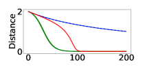
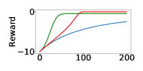
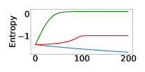
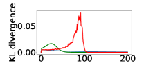
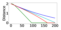
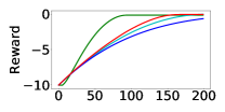
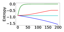
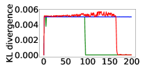
Figure 1: Comparison of different update rules with and without entropy regularization in the toy example of Section 4. The figures show the “Distance” between optimal and current policy mean (see Eq. (17)), the expected “Reward”, the expected “Entropy”, and the expected “KL-divergence” between previous and current policy over $200$ iterations (x-axis). Top: Policy updates with constant learning rates and no trust region. Comparison of the natural gradient (blue), natural gradient with entropy regularization (green) and vanilla policy gradient (red). Bottom: Policy updates with trust region. Comparison of the natural gradient (blue), natural gradient where the entropy is controlled to a set-value (green), natural gradient with zero entropy loss (cyan) and vanilla policy gradient (red). To summarize, without entropy regularization the natural gradient decreases the entropy too fast.

Empirical Evaluation of Trust Region Updates. In the trust region case, we minimized the Lagrange dual at each iteration yielding $\eta$ and $\omega$. We chose at each iteration the highest policy gradient learning rate where the KL-bound was still met. For entropy regularization we tested two setups: 1) We fixed the entropy of the policy (that is, $\gamma=0$), 2) The entropy of the policy was slowly driven to $0$. Figure 1 (bottom) shows the results. The natural gradient still suffers from slow convergence due to decreasing the entropy of the policy gradually. The standard gradient again performs better as it increases the entropy outperforming even the zero entropy loss natural gradient. For entropy control, even more sophisticated scheduling could be used such as the step-size control of CMA-ES (Hansen and Ostermeier, 2001) as a heuristic that works well.

5 Related Work

Similar to classical reinforcement learning the leading contenders in deep reinforcement learning can be divided into value based-function methods such as Q-learning with deep Q-Network (DQN) (Mnih et al., 2015), actor-critic methods (Wu et al., 2017; Tangkaratt et al., 2018; Abdolmaleki et al., 2018), policy gradient methods such as deep deterministic policy gradient (DDPG) (Silver et al., 2014; Lillicrap et al., 2015) and policy search methods based on information theoretic / trust region methods, such as proximal policy optimization (PPO) (Schulman et al., 2017) and trust region policy optimization (TRPO) (Schulman et al., 2015).

Trust region optimization was introduced in the relative entropy policy search (REPS) method (Peters et al., 2010). TRPO and TNPG (Schulman et al., 2015) are the first methods to apply trust region optimization successfully to neural networks. In contrast to TRPO and TNPG, we derive our method from the compatible value function approximation perspective. TRPO and TNPG differ from our approach, in that they do not use an entropy constraint and do not consider the difference between the log-linear and non-linear parameters for their update. On the technical level, compared to TRPO, we can update the log-linear parameters (output layer of neural network and the covariance) with an exact update step while TRPO does a line search to find the update step. Moreover, for the covariance we can find an exact update to enforce a specific entropy and thus control exploration while TRPO does not bound the entropy, only the KL-divergence. PPO also applies an adaptive KL penalty term.

Kakade (2001); Bagnell and Schneider (2003); Peters and Schaal (2008); Geist and Pietquin (2010) have also suggested similar update rules based on the natural gradient for the policy gradient framework. Wu et al. (2017) applied approximate natural gradient updates to both the actor and critic in an actor-critic framework but did not utilize compatible value functions or an entropy bound. Peters and Schaal (2008); Geist and Pietquin (2010) investigated the idea of compatible value functions in combination with the natural gradient but used manual learning rates instead of trust region optimization. The approaches in (Abdolmaleki et al., 2015; Akrour et al., 2016) use an entropy bound similar to ours. However, the approach in (Abdolmaleki et al., 2015) is a stochastic search method, that is, it ignores sequential decisions and views the problem as black-box optimization, and the approach in (Akrour et al., 2016) is restricted to trajectory optimization. Moreover, both of these approaches do not explicitly handle non-linear parameters such as those found in neural networks. The entropy bound used in (Tangkaratt et al., 2018) is similar to ours, however, their method depends on second order approximations of a deep Q-function, resulting in a much more complex policy update that can suffer from the instabilities of learning a non-linear Q-function.

For exploration one can in general add an entropy term to the objective. In the experiments, we compare against TRPO with this additive entropy term. In preliminary experiments, to control entropy in TRPO, we also combined the entropy and KL-divergence constraints into a single constraint without success.

6 Experiments

In the experiments, we focused on investigating the following research question: Does the proposed entropy regularization approach help to improve performance compared to other methods which do not control the entropy explicitly? For selecting comparison methods we followed (Duan et al., 2016) and took four gradient based methods: Trust Region Policy Optimization (TRPO) (Schulman et al., 2015), Truncated Natural Policy Gradient (Duan et al., 2016; Schulman et al., 2015), REINFORCE (VPG) (Williams, 1992), Reward-Weighted Regression (RWR) (Kober and Peters, 2009) and two gradient-free black box optimization methods: Cross Entropy Method (CEM) (Rubinstein, 1999), Covariance Matrix Adaption Evolution Strategy (CMA-ES) (Hansen and Ostermeier, 2001). We used rllab  for algorithm implementation. We ran experiments in both challenging continuous control tasks and discrete partially observable tasks which we discuss next.

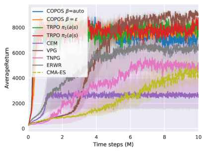
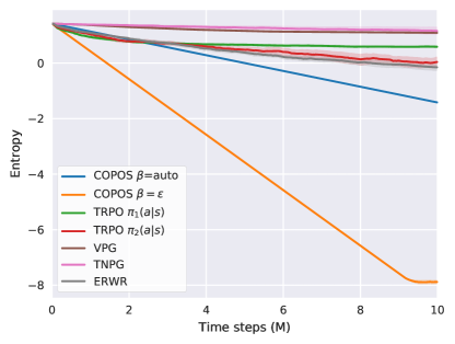
(a) RoboschoolInvertedDoublePendulum-v1
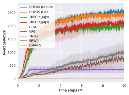
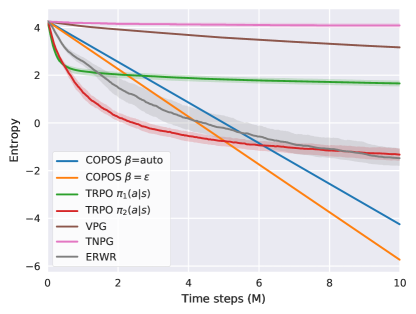
(b) RoboschoolHopper-v1
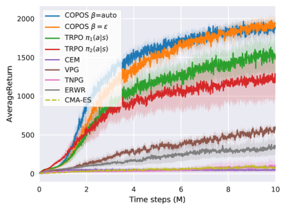
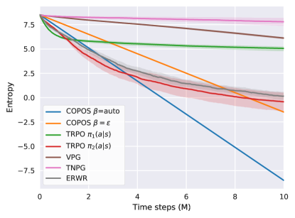
(c) RoboschoolWalker2d-v1
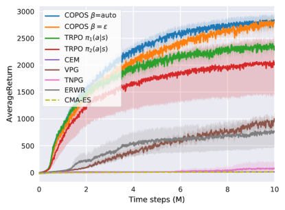
(d) RoboschoolHalfCheetah-v1

Figure 2: Average return and differential entropy over $10$ random seeds of comparison methods in continuous Roboschool tasks (see, Fig. 3 for the other continuous tasks and Table 1 for a summary). Shaded area denotes the bootstrapped $95\%$ confidence interval. Algorithms were executed for $1000$ iterations with $10000$ time steps (samples) in each iteration.

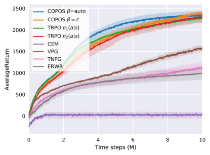
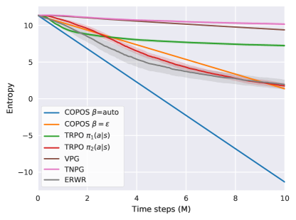
(a) RoboschoolAnt-v1
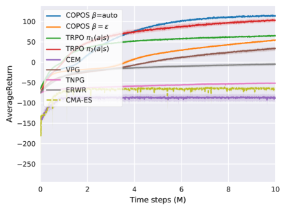
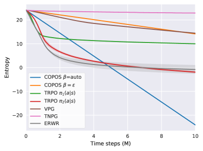
(b) RoboschoolHumanoid-v1
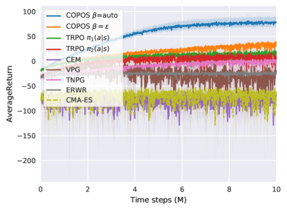
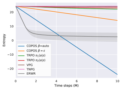
(c) RoboschoolHumanoidFlagrunHarder-v1
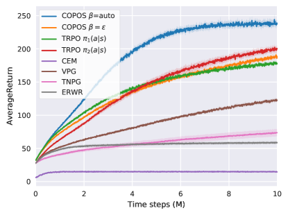
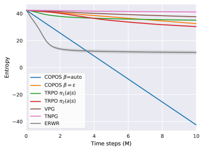
(d) RoboschoolAtlasForwardWalk-v1

Figure 3: Average return and differential entropy of comparison methods over $10$ random seeds in continuous Roboschool tasks (see, Fig. 2 for the other continuous tasks and Table 1 for a summary). Shaded area denotes the bootstrapped $95\%$ confidence interval. Algorithms were executed for $1000$ iterations with $10000$ time steps (samples) in each iteration.

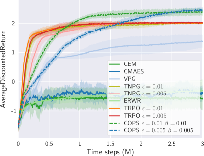
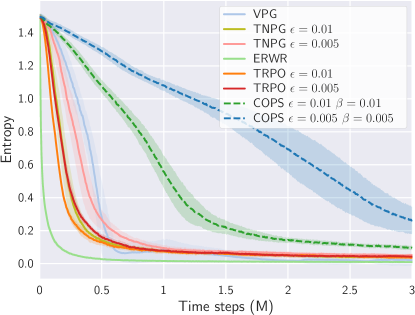
(a) FVRS $(5,7)$ noisy sensor
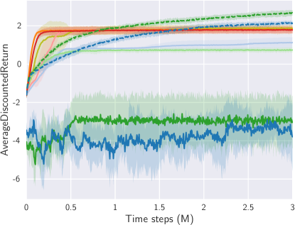
(b) FVRS $(5,7)$ full observations

Figure 4: Average discounted return and Shannon entropy for both FVRS $5\times 7$ with a noisy sensor and full observations over $10$ random seeds. Shaded area denotes the bootstrapped $95\%$ confidence interval. Algorithms were executed for $600$ iterations with $5000$ time steps (samples) in each iteration.

Continuous Tasks. In the continuous case, we ran experiments in eight different Roboschool  environments which provide continuous control tasks of increasing difficulty and action dimensions without requiring a paid license.

We ran all evaluations, $10$ random seeds for each method, for $1000$ iterations of $10000$ samples each. In all problems, we used the Gaussian policy defined in Eq. (8) for COPOS and TRPO (denoted by $\pi_{1}(a|s)$) with $\max(10,\textrm{action dimensions})$ neural network outputs as basis functions, a neural network with two hidden layers each containing $32$ tanh-neurons, and a diagonal precision matrix. For TRPO and other methods, except COPOS, we also evaluated a policy, denoted for TRPO by $\pi_{2}(a|s)$, where the neural network directly specifies the mean and the diagonal covariance is parameterized with log standard deviations. In the experiments, we used high identical initial variances (we tried others without success) for all policies. We set $\epsilon=0.01$ (Schulman et al., 2015) in all experiments. For COPOS we used two equality entropy constraints: $\beta=\epsilon$ and $\beta=$auto. In $\beta=$auto, we assume positive initial entropy and schedule the entropy to be the negative initial entropy after $1000$ iterations. Since we always initialize the variances to one, higher dimensional problems have higher initial entropy. Thus $\beta=$auto reduces the entropy faster for high dimensional problems effectively scaling the reduction with dimensionality. Table 1 summarizes the results in continuous tasks: COPOS outperforms comparison methods in most of the environments. Fig. 2 and Fig. 3 show learning curves and performance of COPOS compared to the other methods. COPOS prevents both too fast, and, too slow entropy reduction while outperforming comparison methods. Table 4 in Appendix C shows additional results for experiments where different constant entropy bonuses were added to the objective function of TRPO without success, highlighting the necessity of principled entropy control.

Discrete control task. Partial observability often requires efficient exploration due to non-myopic actions yielding long term rewards which is challenging for model-free methods. The Field Vision Rock Sample (FVRS) (Ross et al., 2008) task is a partially observable Markov decision process (POMDP) benchmark task. For the discrete action experiments we used as policy a softmax policy with a fully connected feed forward neural network consisting of 2 hidden layers with 30 tanh nonlinearities each. The input to the neural network is the observation history and the current position of the agent in the grid. To obtain the hyperparameters $\beta$, $\epsilon$, and the scaling factor for TRPO with additive entropy regularization, denoted with “TRPO ent reg”, we performed a grid search on smaller instances of FVRS. See Appendix B for more details about the setup. Results in Table 2 and Figure 4 show that COPOS outperforms the comparison methods due to maintaining higher entropy. FVRS has been used with model-based online POMDP algorithms (Ross et al., 2008) but not with model-free algorithms. The best model-based results in (Ross et al., 2008) (scaled to correspond to our rewards, COPOS in parentheses) are $2.275$ ($1.94$) in FVRS(5,5) and $2.34$ ($2.45$) in FVRS(5,7).

7 Conclusions & Future Work

We showed that when we use the natural parameterization of a standard exponential policy distribution in combination with compatible value function approximation, the natural gradient and trust region optimization are equivalent. Furthermore, we demonstrated that natural gradient updates may reduce the entropy of the policy according to a schedule which can lead to premature convergence. To combat the problem of bad entropy scheduling in trust region methods we proposed a new compatible policy search method called COPOS that can control the entropy of the policy using an entropy bound. In both challenging high dimensional continuous and discrete tasks the approach yielded state-of-the-art results due to better entropy control. In future work, an exciting direction is to apply efficient approximations to compute the natural gradient (Bernacchia et al., 2018). Moreover, we have started work on applying the proposed algorithm in challenging partially observable environments found for example in autonomous driving where exploration and sample efficiency is crucial for finding high quality policies (Dosovitskiy et al., 2017).

Table 1: Continuous control environments. Mean of the average return over $50$ last iterations $\pm$ standard error over $10$ random seeds. Bold denotes: no statistically significant difference to the best result (Welch’s t-test with $p<0.05$).

	COPOS $\beta$=auto	COPOS $\beta$=$\epsilon$	TRPO $\pi_{1}(\boldsymbol{a}|\boldsymbol{s})$
RoboInvertedDoublePendulum-v1	7107 $\pm$ 416	7722 $\pm$ 235.3	7904 $\pm$ 192.4
RoboHopper-v1	2514 $\pm$ 35.11	2427 $\pm$ 47.96	2005 $\pm$ 26.04
RoboWalker2d-v1	1878 $\pm$ 34.59	1906 $\pm$ 41.48	1518 $\pm$ 93.11
RoboHalfCheetah-v1	2804 $\pm$ 57.27	2772 $\pm$ 42.23	2341 $\pm$ 16.52
RoboAnt-v1	2335 $\pm$ 49.69	2375 $\pm$ 26.88	2263 $\pm$ 48.09
RoboHumanoid-v1	113.85 $\pm$ 0.94	52.92 $\pm$ 0.31	64.77 $\pm$ 0.38
RoboHumanoidFlagrunHarder-v1	77.72 $\pm$ 4.86	32.14 $\pm$ 1.34	14.51 $\pm$ 1.25
RoboAtlasForwardWalk-v1	238.1 $\pm$ 2.08	186.8 $\pm$ 1.18	177.7 $\pm$ 0.44

	TRPO $\pi_{2}(\boldsymbol{a}|\boldsymbol{s})$	CMA-ES	VPG
RoboInvertedDoublePendulum-v1	8052 $\pm$ 172.3	4382 $\pm$ 379.2	9020 $\pm$ 35.10
RoboHopper-v1	2106 $\pm$ 85.59	25.87 $\pm$ 8.66	751.4 $\pm$ 145.4
RoboWalker2d-v1	1223 $\pm$ 139.0	82.38 $\pm$ 9.72	559.7 $\pm$ 13.55
RoboHalfCheetah-v1	2024 $\pm$ 261.2	13.38 $\pm$ 3.88	918.1 $\pm$ 43.57
RoboAnt-v1	2291 $\pm$ 65.66	Out of Memory	1558 $\pm$ 35.71
RoboHumanoid-v1	102.5 $\pm$ 2.16	-65.07 $\pm$ 1.71	32.72 $\pm$ 2.47
RoboHumanoidFlagrunHarder-v1	5.04 $\pm$ 2.70	-74.62 $\pm$ 3.28	-31.62 $\pm$ 4.59
RoboAtlasForwardWalk-v1	198.4 $\pm$ 1.94	Out of Memory	121.5 $\pm$ 0.92

	CEM	TNPG	ERWR
RoboInvertedDoublePendulum-v1	2643 $\pm$ 628.9	4866 $\pm$ 1178	6367 $\pm$ 937.4
RoboHopper-v1	346.6 $\pm$ 66.89	20.55 $\pm$ 2.42	985.1 $\pm$ 173.1
RoboWalker2d-v1	49.03 $\pm$ 10.69	90.36 $\pm$ 35.52	333.3 $\pm$ 47.73
RoboHalfCheetah-v1	11.27 $\pm$ 2.93	72.22 $\pm$ 56.48	747.3 $\pm$ 137.8
RoboAnt-v1	25.17 $\pm$ 35.09	1102 $\pm$ 64.61	982.6 $\pm$ 74.23
RoboHumanoid-v1	-87.19 $\pm$ 4.21	-51.39 $\pm$ 1.01	-4.95 $\pm$ 2.16
RoboHumanoidFlagrunHarder-v1	-78.00 $\pm$ 4.74	-0.25 $\pm$ 0.68	-24.59 $\pm$ 0.65
RoboAtlasForwardWalk-v1	14.90 $\pm$ 0.60	72.96 $\pm$ 2.75	58.54 $\pm$ 1.07

Table 2: Average discounted return on discrete control FVRS instances (fully and partially observable). Bold denotes: no statistically significant difference to the best result (Welch’s t-test with $p<0.05$).

	COPOS	TRPO	TRPO ent reg	TNPG
$5\times 5$ full	2.14 $\pm$ 0.08	1.50 $\pm$ 0.23	1.47 $\pm$ 0.22	1.43 $\pm$ 0.28
$5\times 5$ noise	1.94 $\pm$ 0.12	1.24 $\pm$ 0.02	1.24 $\pm$ 0.01	1.24 $\pm$ 0.01
$5\times 7$ full	2.66 $\pm$ 0.14	1.80 $\pm$ 0.20	1.92 $\pm$ 0.17	1.87 $\pm$ 0.16
$5\times 7$ noise	2.45 $\pm$ 0.10	2.01 $\pm$ 0.02	2.02 $\pm$ 0.02	2.01 $\pm$ 0.03
$7\times 8$ full	1.66 $\pm$ 0.17	1.28 $\pm$ 0.32	1.31 $\pm$ 0.20	1.19 $\pm$ 0.26
$7\times 8$ noise	1.32 $\pm$ 0.15	1.22 $\pm$ 0.28	1.36 $\pm$ 0.16	1.18 $\pm$ 0.22

Appendix

Appendix A Solution for the Lagrange Multipliers

In order to compute a solution to the optimization objective with a KL-divergence and an entropy bound, we solve, using the dual of the problem, for the Lagrange multipliers associated with the bounds. We first discuss for the continuous action case how we optimize the multipliers exactly in the case of only log-linear parameters, continue with how we find an approximate solution in the case of also non-linear parameters, and then discuss the discrete action case.

A.1 Computing Lagrange Multipliers $\eta$ and $\omega$ for log-linear Parameters

Minimize the dual of the optimization objective (see e.g. Akrour et al. [2016] for a similar dual)

$$g_{t}(\eta,\omega) =\eta\epsilon-\omega\beta+(\eta+\omega)\int\tilde{p}_{t}(\boldsymbol{s})\log\left(\int\pi(\boldsymbol{a}|\boldsymbol{s})^{\eta/(\eta+\omega)}\exp\left(\tilde{Q}_{t}(\boldsymbol{s},\boldsymbol{a})/(\eta+\omega)\right)d\boldsymbol{a}\right)d\boldsymbol{s}$$ (18)

w.r.t. $\eta$ and $\omega$. Note that action independent parts of $\log\pi(\boldsymbol{a}|\boldsymbol{s})$ in Eq. (18) do not have an effect on the choice of $\eta$ and $\omega$ and we will discard them.

For a Gaussian policy

$$\pi(\boldsymbol{a}|\boldsymbol{s})=\mathcal{N}\left(\boldsymbol{a}\Bigg{|}\boldsymbol{\mu}=\boldsymbol{K}\boldsymbol{\varphi}(\boldsymbol{s})=\sum_{i}\varphi_{i}(\boldsymbol{s})\boldsymbol{k}_{i},\boldsymbol{\Sigma}\right)$$ (19)

we get

$$\tilde{Q}_{t}(s,a) =\boldsymbol{\psi}(\boldsymbol{s},\boldsymbol{a})^{T}\boldsymbol{w}=\begin{bmatrix}-\textrm{vec}[0.5\boldsymbol{a}\boldsymbol{a}^{T}]\\ \textrm{vec}[\boldsymbol{a}\boldsymbol{\varphi}(\boldsymbol{s})^{T}]\end{bmatrix}^{T}\begin{bmatrix}\boldsymbol{w}_{1}\\ \boldsymbol{w}_{2}\end{bmatrix}=-0.5\boldsymbol{a}^{T}\boldsymbol{W}_{aa}\boldsymbol{a}+\boldsymbol{\varphi}(\boldsymbol{s})^{T}\boldsymbol{W}_{sa}\boldsymbol{a}$$ (20)

$$g_{t}(\eta,\omega) =\eta\epsilon-\omega\beta+(\eta+\omega)\int\tilde{p}_{t}(\boldsymbol{s})\log\Bigg{(}\int C_{\pi}^{\frac{\eta}{\eta+\omega}}\exp\left(-0.5\eta/(\eta+\omega)(\boldsymbol{a}-\boldsymbol{\mu})^{T}\boldsymbol{\Sigma}^{-1}(\boldsymbol{a}-\boldsymbol{\mu})\right)$$

$$\exp\left(-0.5\boldsymbol{a}^{T}\boldsymbol{W}_{aa}/(\eta+\omega)\boldsymbol{a}+\boldsymbol{\varphi}(\boldsymbol{s})^{T}\boldsymbol{W}_{sa}/(\eta+\omega)\boldsymbol{a}\right)d\boldsymbol{a}\Bigg{)}d\boldsymbol{s}$$ (21)

$$g_{t}(\eta,\omega) =\eta\epsilon-\omega\beta+(\eta+\omega)\int\tilde{p}_{t}(\boldsymbol{s})\log\Bigg{(}\int C_{\pi}^{\frac{\eta}{\eta+\omega}}$$

$$\quad\exp\left(\frac{\eta}{\eta+\omega}(-0.5\boldsymbol{a}^{T}\boldsymbol{\Sigma}^{-1}\boldsymbol{a}+\boldsymbol{\mu}^{T}\boldsymbol{\Sigma}^{-1}\boldsymbol{a}-0.5\boldsymbol{\mu}^{T}\boldsymbol{\Sigma}^{-1}\mu)\right)$$

$$\quad\exp\left(-0.5\boldsymbol{a}^{T}\boldsymbol{W}_{aa}/(\eta+\omega)\boldsymbol{a}+\boldsymbol{\varphi}(\boldsymbol{s})^{T}\boldsymbol{W}_{sa}/(\eta+\omega)\boldsymbol{a}\right)d\boldsymbol{a}\Bigg{)}d\boldsymbol{s}$$ (22)

$$g_{t}(\eta,\omega) =\eta\epsilon-\omega\beta+(\eta+\omega)\int\tilde{p}_{t}(\boldsymbol{s})\log\Bigg{(}\int C_{\pi}^{\frac{\eta}{\eta+\omega}}\exp\Bigg{(}\frac{1}{\eta+\omega}\Bigg{(}-0.5\boldsymbol{a}^{T}\Big{(}\eta\boldsymbol{\Sigma}^{-1}+\boldsymbol{W}_{aa}\Big{)}\boldsymbol{a}$$

$$\quad+\Big{(}\eta\boldsymbol{\varphi}(\boldsymbol{s})^{T}\boldsymbol{K}^{T}\boldsymbol{\Sigma}^{-1}+\boldsymbol{\varphi}(\boldsymbol{s})^{T}\boldsymbol{W}_{sa}\Big{)}\boldsymbol{a}-0.5\eta\boldsymbol{\varphi}(\boldsymbol{s})^{T}\boldsymbol{K}^{T}\boldsymbol{\Sigma}^{-1}\boldsymbol{K}\boldsymbol{\varphi}(\boldsymbol{s})\Bigg{)}\Bigg{)}d\boldsymbol{a}\Bigg{)}d\boldsymbol{s}$$ (23)

$$g_{t}(\eta,\omega) =\eta\epsilon-\omega\beta+(\eta+\omega)\int\tilde{p}_{t}(\boldsymbol{s})\log\Bigg{(}\int C_{\pi}^{\frac{\eta}{\eta+\omega}}$$

$$\quad\exp\left(\frac{1}{\eta+\omega}\left(-0.5\boldsymbol{a}^{T}\boldsymbol{H}_{aa}\boldsymbol{a}+\boldsymbol{\varphi}(\boldsymbol{s})^{T}\boldsymbol{H}_{sa}\boldsymbol{a}-0.5\boldsymbol{\varphi}(\boldsymbol{s})^{T}\boldsymbol{H}_{ss}\boldsymbol{\varphi}(\boldsymbol{s})\right)\right)d\boldsymbol{a}\Bigg{)}d\boldsymbol{s}$$ (24)

$$g_{t}(\eta,\omega) =\eta\epsilon-\omega\beta+(\eta+\omega)\int\tilde{p}_{t}(\boldsymbol{s})\log\Bigg{(}\int C_{\pi}^{\frac{\eta}{\eta+\omega}}$$

$$\quad\exp\Big{(}\frac{1}{\eta+\omega}\Big{(}-0.5(\boldsymbol{a}-\boldsymbol{H}_{aa}^{-1}\boldsymbol{H}_{sa}^{T}\boldsymbol{\varphi}(\boldsymbol{s}))^{T}\boldsymbol{H}_{aa}(\boldsymbol{a}-\boldsymbol{H}_{aa}^{-1}\boldsymbol{H}_{sa}^{T}\boldsymbol{\varphi}(\boldsymbol{s}))$$

$$\quad\quad+0.5\boldsymbol{\varphi}(\boldsymbol{s})^{T}\boldsymbol{H}_{sa}\boldsymbol{H}_{aa}^{-1}\boldsymbol{H}_{sa}^{T}\boldsymbol{\varphi}(\boldsymbol{s})-0.5\boldsymbol{\varphi}(\boldsymbol{s})^{T}\boldsymbol{H}_{ss}\boldsymbol{\varphi}(\boldsymbol{s})\Big{)}\Big{)}d\boldsymbol{a}\Bigg{)}d\boldsymbol{s}$$ (25)

$$g_{t}(\eta,\omega) =\eta\epsilon-\omega\beta+(\eta+\omega)\int\tilde{p}_{t}(\boldsymbol{s})\log\Bigg{(}\exp\Big{(}\frac{1}{\eta+\omega}\Big{(}0.5\boldsymbol{\varphi}(\boldsymbol{s})^{T}(\boldsymbol{H}_{sa}\boldsymbol{H}_{aa}^{-1}\boldsymbol{H}_{sa}^{T}-\boldsymbol{H}_{ss})\boldsymbol{\varphi}(\boldsymbol{s})\Big{)}\Big{)}$$

$$((2\pi)^{-k/2}|\boldsymbol{\Sigma}|^{-0.5})^{\frac{\eta}{\eta+\omega}}/((2\pi)^{-k/2}|(\eta+\omega)\boldsymbol{H}_{aa}^{-1}|^{-0.5})\Bigg{)}d\boldsymbol{s}$$ (26)

$$g_{t}(\eta,\omega) =\eta\epsilon-\omega\beta+(\eta+\omega)\int\tilde{p}_{t}(\boldsymbol{s})\Big{(}\frac{1}{\eta+\omega}0.5\boldsymbol{\varphi}(\boldsymbol{s})^{T}(\boldsymbol{H}_{sa}\boldsymbol{H}_{aa}^{-1}\boldsymbol{H}_{sa}^{T}-\boldsymbol{H}_{ss})\boldsymbol{\varphi}(\boldsymbol{s})$$

$$\quad+\frac{\eta}{\eta+\omega}\log((2\pi)^{-k/2}|\boldsymbol{\Sigma}|^{-0.5})-\log((2\pi)^{-k/2}|(\eta+\omega)\boldsymbol{H}_{aa}^{-1}|^{-0.5})\Big{)}d\boldsymbol{s},$$ (27)

$$g_{t}(\eta,\omega) =\eta\epsilon-\omega\beta+\int\tilde{p}_{t}(\boldsymbol{s})\Big{(}0.5\boldsymbol{\varphi}(\boldsymbol{s})^{T}(\boldsymbol{H}_{sa}\boldsymbol{H}_{aa}^{-1}\boldsymbol{H}_{sa}^{T}-\boldsymbol{H}_{ss})\boldsymbol{\varphi}(\boldsymbol{s})\Big{)}d\boldsymbol{s}$$

$$\quad+\eta\log((2\pi)^{-k/2}|\boldsymbol{\Sigma}|^{-0.5})-(\eta+\omega)\log((2\pi)^{-k/2}|(\eta+\omega)\boldsymbol{H}_{aa}^{-1}|^{-0.5}),$$ (28)

$$g_{t}(\eta,\omega) =\eta\epsilon-\omega\beta+\int\tilde{p}_{t}(\boldsymbol{s})\Big{(}0.5\boldsymbol{\varphi}(\boldsymbol{s})^{T}(\boldsymbol{H}_{sa}\boldsymbol{H}_{aa}^{-1}\boldsymbol{H}_{sa}^{T}-\boldsymbol{H}_{ss})\boldsymbol{\varphi}(\boldsymbol{s})\Big{)}d\boldsymbol{s}$$

$$\quad-0.5\eta\log|2\pi\boldsymbol{\Sigma}|+0.5(\eta+\omega)\log|2\pi(\eta+\omega)\boldsymbol{H}_{aa}^{-1}|,$$ (29)

where

$$\boldsymbol{H}_{aa} =\eta\boldsymbol{\Sigma}^{-1}+\boldsymbol{W}_{aa}$$ (30)

$$\boldsymbol{H}_{sa} =\eta\boldsymbol{K}^{T}\boldsymbol{\Sigma}^{-1}+\boldsymbol{W}_{sa}$$ (31)

$$\boldsymbol{H}_{ss} =\eta\boldsymbol{K}^{T}\boldsymbol{\Sigma}^{-1}\boldsymbol{K}$$ (32)

and $k$ is the dimensionality of actions. We got the end result by completing the square.

A.2 Computing $\eta$ and $\omega$ for non-linear parameters

Similarly to the log-linear parameters we minimize the dual

$$g_{t}(\eta,\omega) =\eta\epsilon-\omega\beta+(\eta+\omega)\int\tilde{p}_{t}(\boldsymbol{s})\log\left(\int\pi(\boldsymbol{a}|\boldsymbol{s})^{\eta/(\eta+\omega)}\exp\left(\tilde{Q}_{t}(\boldsymbol{s},\boldsymbol{a})/(\eta+\omega)\right)d\boldsymbol{a}\right)d\boldsymbol{s}$$ (34)

w.r.t. $\eta$ and $\omega$. As before action independent parts of $\log\pi(\boldsymbol{a}|\boldsymbol{s})$ in Eq. (18) do not have an effect on the choice of $\eta$ and $\omega$ and we will discard them.

In our Linear Gaussian policy with constant covariance

$$\pi(\boldsymbol{a}|\boldsymbol{s})=\mathcal{N}\left(\boldsymbol{a}\Bigg{|}\boldsymbol{\mu}=\boldsymbol{K}\boldsymbol{\varphi}(\boldsymbol{s})=\sum_{i}\varphi_{i}(\boldsymbol{s})\boldsymbol{k}_{i},\boldsymbol{\Sigma}\right),$$ (35)

we have

$$\log\pi(\boldsymbol{a}|\boldsymbol{s}) =-0.5\boldsymbol{\varphi}(\boldsymbol{s})^{T}\boldsymbol{U}\boldsymbol{K}\boldsymbol{\varphi}(\boldsymbol{s})+\boldsymbol{\varphi}(\boldsymbol{s})^{T}\boldsymbol{U}\boldsymbol{a}-0.5\boldsymbol{a}^{T}\boldsymbol{\Sigma}^{-1}\boldsymbol{a}+\textrm{const},$$ (36)

where $\textrm{const}=-\sqrt{(2\pi)^{k}|\boldsymbol{\Sigma}|}$ and $\boldsymbol{U}=\boldsymbol{K}^{T}\boldsymbol{\Sigma}^{-1}$. Therefore,

$$\nabla_{\boldsymbol{\beta}}\log\pi_{\boldsymbol{\beta},\boldsymbol{\theta}}(\boldsymbol{a}|\boldsymbol{s}) =\frac{\partial}{\partial\boldsymbol{\beta}}\boldsymbol{\varphi}(\boldsymbol{s})^{T}\boldsymbol{U}\boldsymbol{a}-\frac{\partial}{\partial\boldsymbol{\beta}}0.5\boldsymbol{\varphi}(\boldsymbol{s})^{T}\boldsymbol{U}\boldsymbol{K}\boldsymbol{\varphi}(\boldsymbol{s}),$$ (37)

where we are able to split the equation into action-value and value parts depending on whether they depend on $\boldsymbol{a}$. Using the action-value part $\frac{\partial}{\partial\boldsymbol{\beta}}\boldsymbol{\varphi}(\boldsymbol{s})^{T}\boldsymbol{U}\boldsymbol{a}$ to estimate $\boldsymbol{w}_{3}$ we get

$$\tilde{Q}_{t}(s,a) =\boldsymbol{\psi}(\boldsymbol{s},\boldsymbol{a})^{T}\boldsymbol{w}=\begin{bmatrix}-\textrm{vec}[0.5\boldsymbol{a}\boldsymbol{a}^{T}]\\ \textrm{vec}[\boldsymbol{a}\boldsymbol{\varphi}(\boldsymbol{s})^{T}]\\ \frac{\partial}{\partial\boldsymbol{\beta}}\boldsymbol{\varphi}(\boldsymbol{s})^{T}\boldsymbol{U}\boldsymbol{a}\end{bmatrix}^{T}\begin{bmatrix}\boldsymbol{w}_{1}\\ \boldsymbol{w}_{2}\\ \boldsymbol{w}_{3}\end{bmatrix}=-0.5\boldsymbol{a}^{T}\boldsymbol{W}_{aa}\boldsymbol{a}+\boldsymbol{\varphi}(\boldsymbol{s})^{T}\boldsymbol{W}_{sa}\boldsymbol{a}+\boldsymbol{w}_{a}(s)^{T}\boldsymbol{a},$$ (38)

where $\boldsymbol{w}_{a}(s)^{T}=\boldsymbol{w}_{3}^{T}\frac{\partial\boldsymbol{\varphi}(\boldsymbol{s})^{T}}{\partial\boldsymbol{\beta}}\boldsymbol{U}$. By completing the square we get

$$g_{t}(\eta,\omega) =\eta\epsilon-\omega\beta+(\eta+\omega)\int\tilde{p}_{t}(\boldsymbol{s})\log\Bigg{(}\int C_{\pi}^{\frac{\eta}{\eta+\omega}}\exp\left(-0.5\eta/(\eta+\omega)(\boldsymbol{a}-\boldsymbol{\mu})^{T}\boldsymbol{\Sigma}^{-1}(\boldsymbol{a}-\boldsymbol{\mu})\right)$$

$$\exp\left(-0.5\boldsymbol{a}^{T}\boldsymbol{W}_{aa}/(\eta+\omega)\boldsymbol{a}+(\boldsymbol{\varphi}(\boldsymbol{s})^{T}\boldsymbol{W}_{sa}+\boldsymbol{w}_{a}(s)^{T})/(\eta+\omega)\boldsymbol{a}\right)d\boldsymbol{a}\Bigg{)}d\boldsymbol{s}$$ (40)

$$g_{t}(\eta,\omega) =\eta\epsilon-\omega\beta+(\eta+\omega)\int\tilde{p}_{t}(\boldsymbol{s})\log\Bigg{(}\int C_{\pi}^{\frac{\eta}{\eta+\omega}}\exp\Bigg{(}\frac{1}{\eta+\omega}\Bigg{(}-0.5\boldsymbol{a}^{T}\Big{(}\eta\boldsymbol{\Sigma}^{-1}+\boldsymbol{W}_{aa}\Big{)}\boldsymbol{a}$$

$$\quad+\Big{(}\eta\boldsymbol{\varphi}(\boldsymbol{s})^{T}\boldsymbol{K}^{T}\boldsymbol{\Sigma}^{-1}+(\boldsymbol{\varphi}(\boldsymbol{s})^{T}\boldsymbol{W}_{sa}+\boldsymbol{w}_{a}(s)^{T})\Big{)}\boldsymbol{a}-0.5\eta\boldsymbol{\varphi}(\boldsymbol{s})^{T}\boldsymbol{K}^{T}\boldsymbol{\Sigma}^{-1}\boldsymbol{K}\boldsymbol{\varphi}(\boldsymbol{s})\Bigg{)}\Bigg{)}d\boldsymbol{a}\Bigg{)}d\boldsymbol{s}$$ (41)

$$g_{t}(\eta,\omega) =\eta\epsilon-\omega\beta+\int\tilde{p}_{t}(\boldsymbol{s})\Big{(}0.5(\boldsymbol{h}_{a}(\boldsymbol{s})^{T}\boldsymbol{H}_{aa}^{-1}\boldsymbol{h}_{a}(\boldsymbol{s})-h_{ss}(\boldsymbol{s}))d\boldsymbol{s}$$

$$\quad-0.5\eta\log|2\pi\boldsymbol{\Sigma}|+0.5(\eta+\omega)\log|2\pi(\eta+\omega)\boldsymbol{H}_{aa}^{-1}|,$$ (42)

where

$$\boldsymbol{H}_{aa} =\eta\boldsymbol{\Sigma}^{-1}+\boldsymbol{W}_{aa}$$ (43)

$$\boldsymbol{h}_{a}(\boldsymbol{s}) =\eta\boldsymbol{\varphi}(\boldsymbol{s})^{T}\boldsymbol{K}^{T}\boldsymbol{\Sigma}^{-1}+\boldsymbol{\varphi}(\boldsymbol{s})^{T}\boldsymbol{W}_{sa}+\boldsymbol{w}_{a}(s)^{T}$$ (44)

$$h_{ss}(\boldsymbol{s}) =\eta\varphi(\boldsymbol{s})^{T}\boldsymbol{K}^{T}\boldsymbol{\Sigma}^{-1}\boldsymbol{K}\boldsymbol{\varphi}(\boldsymbol{s})$$ (45)

and $k$ is the dimensionality of actions.

A.3 Derivation of the dual for the discrete action case

To derive the dual of our trust region optimization problem with entropy regularization and discrete actions we start with following program, where we replaced the expectation with integrals and use the compatible value function for the returns.

$$\textrm{argmax}_{\pi_{\boldsymbol{\theta}}} \;\int p(\boldsymbol{s})\int\pi_{\boldsymbol{\theta}}(\boldsymbol{a}|\boldsymbol{s})\;\tilde{G}^{\pi_{\textrm{old}}}_{\boldsymbol{w}}(\boldsymbol{s},\boldsymbol{a})\;d\boldsymbol{a}\;d\boldsymbol{s}$$ (47)

subject to $$\;\int p(\boldsymbol{s})\int KL\left(\pi_{\boldsymbol{\theta}}(\boldsymbol{a}|\boldsymbol{s})\;||\;\pi_{\boldsymbol{\theta}_{\text{old}}}(\boldsymbol{a}|\boldsymbol{s})\right)\;d\boldsymbol{a}\;d\boldsymbol{s}<\epsilon$$

$$\;\int p(\boldsymbol{s})\int H\left(\pi_{\boldsymbol{\theta}}(\boldsymbol{a}|\boldsymbol{s})\right)-H\left(\pi_{\boldsymbol{\theta}_{\text{old}}}(\boldsymbol{a}|\boldsymbol{s})\right)\;d\boldsymbol{a}\;d\boldsymbol{s}<\beta$$

$$1=\int\int p(\boldsymbol{s})\pi_{\boldsymbol{\theta}}(\boldsymbol{a}|\boldsymbol{s})\;d\boldsymbol{a}\;d\boldsymbol{s}$$

Since we are in the discrete action case we will be using sums for the brevity of the derivation, but the same derivation can be also done with integrals. Using the method of Lagrange multipliers Boyd and Vandenberghe [2004], we obtain following Lagrange

$$L(\pi(\boldsymbol{a}|\boldsymbol{s}),\eta,\omega,\lambda) =-\sum_{\boldsymbol{s},\boldsymbol{a}}p(\boldsymbol{s})\pi(\boldsymbol{a}|\boldsymbol{s})\tilde{G}^{\pi_{old}}_{w}(\boldsymbol{a},\boldsymbol{s})$$ (48)

$$\quad+\;\eta\left[\sum_{\boldsymbol{s}}p(\boldsymbol{s})\sum_{\boldsymbol{a}}\pi(\boldsymbol{a}|\boldsymbol{s})\log\left(\frac{\pi(\boldsymbol{a}|\boldsymbol{s})}{\pi_{\textrm{old}}(\boldsymbol{a}|\boldsymbol{s})}\right)-\epsilon\right]$$

$$\quad+\;\omega\left[\sum_{\boldsymbol{s},\boldsymbol{a}}p(\boldsymbol{s})H(\pi_{\textrm{old}}(\boldsymbol{a}|\boldsymbol{s}))+\sum_{\boldsymbol{s},\boldsymbol{a}}p(\boldsymbol{s})\pi(\boldsymbol{a}|\boldsymbol{s})\log(\pi(\boldsymbol{a}|\boldsymbol{s}))-\beta\right]$$

$$\quad+\;\lambda\left[\sum_{\boldsymbol{s},\boldsymbol{a}}p(\boldsymbol{s})\pi(\boldsymbol{a}|\boldsymbol{s})-1\right]$$

We differentiate now the Lagrange with respect to $\pi(\boldsymbol{a}|\boldsymbol{s})$ and obtain following system

$$\delta_{\pi(\boldsymbol{a}|\boldsymbol{s})}L =p(\boldsymbol{s})\left[-\tilde{G}^{\pi_{\textrm{old}}}_{\boldsymbol{w}}(\boldsymbol{s},\boldsymbol{a})+\eta\log\left(\frac{\pi(\boldsymbol{a}|\boldsymbol{s})}{\pi_{\textrm{old}}(\boldsymbol{a}|\boldsymbol{s})}\right)+\eta+\omega\log(\pi(\boldsymbol{a}|\boldsymbol{s}))+\omega+\lambda\right].$$ (50)

Setting it to zero and rearranging terms results in

$$\pi(\boldsymbol{a}|\boldsymbol{s}) =\pi_{\textrm{old}}(\boldsymbol{a}|\boldsymbol{s})^{\frac{\eta}{\eta+\omega}}\exp\left(\frac{\tilde{G}^{\pi_{\textrm{old}}}_{\boldsymbol{w}}(\boldsymbol{s},\boldsymbol{a})}{\eta+\omega}\right)\exp\left(\frac{-\eta-\omega-\lambda}{\eta+\omega}\right)$$ (51)

where the last term can be seen as a normalization constant

$$\exp\left(\frac{-\eta-\omega-\lambda}{\eta+\omega}\right) =\left(\sum_{\boldsymbol{a}}\pi_{\textrm{old}}(\boldsymbol{a}|\boldsymbol{s})^{\frac{\eta}{\eta+\omega}}\exp\left(\frac{\tilde{G}^{\pi_{\textrm{old}}}_{\boldsymbol{w}}(\boldsymbol{a},\boldsymbol{s})}{\eta+\omega}\right)\right)^{-1}.$$ (52)

Plugging Eq. (51) and Eq. (52) into Eq. (48) results in the dual (similar to Akrour et al. [2016]) used for optimization

$$L(\eta,\omega)= -\eta\epsilon-\omega\beta+\omega\sum_{\boldsymbol{s},\boldsymbol{a}}p(\boldsymbol{s})H(\pi_{\textrm{old}}(\boldsymbol{a}|\boldsymbol{s}))$$

$$-(\eta+\omega)\sum_{\boldsymbol{s}}p(\boldsymbol{s})\log\left(\sum_{\boldsymbol{a}}\pi_{\textrm{old}}(\boldsymbol{a}|\boldsymbol{s})^{\frac{\eta}{\eta+\omega}}\exp\left(\frac{\tilde{G}^{\pi_{\textrm{old}}}_{\boldsymbol{w}}(\boldsymbol{a},\boldsymbol{s})}{\eta+\omega}\right)\right).$$

Appendix B Technical Details for Discrete Action Experiments

Here, we provide details on the experiments with discrete actions. Table 3 shows details on the hyper-parameters used in the Field Vision RockSample (FVRS) experiments and Algorithm 2 describes details on the discrete action algorithm.

	$(5,5)$ full	$(5,5)$ noise	$(5,7)$ full	$(5,7)$ noise	$(7,8)$ full	$(7,8)$ noise
Input space dim.	15	85	17	115	22	134
Output space dim.	5	5	5	5	5	5
# policy parameters	1410	3510	1650	4560	1620	4980
Sim. step per iteration	5000	5000	5000	5000	5000	5000
Total num. of iterations	600	600	600	600	600	600
Discount $\gamma$	0.95	0.95	0.95	0.95	0.95	0.95
History Length	1	15	1	15	1	15
Horizon	25	25	35	35	50	50

Table 3: Parameters used for FVRS instances

Initialize policy network $\pi_{\boldsymbol{\theta},\boldsymbol{\beta}}$ with non-linear parameters $\boldsymbol{\beta}$ and linear parameters $\boldsymbol{\theta}$ and $\Theta=(\boldsymbol{\theta},\boldsymbol{\beta})$

for episode $\leftarrow 1$ to maxEpisode do

     Initialize empty batch $\mathcal{B}$ 

     while collected samples $<$ batchsize do

          Run policy $\pi_{\boldsymbol{\theta},\boldsymbol{\beta}}(\boldsymbol{a}|\boldsymbol{s})$ for $T$ timesteps or until termination: Draw action $\boldsymbol{a_{t}}\sim\pi_{\boldsymbol{\theta},\boldsymbol{\beta}}(\boldsymbol{a_{t}}|\boldsymbol{s_{t}})$, observe reward $r_{t}$

         Add samples $(\boldsymbol{s_{t}},\boldsymbol{a_{t}},r_{t})$ to $\mathcal{B}$

     end while

     Compute advantage values $A^{\pi_{\text{old}}}(\boldsymbol{s}_{i},\boldsymbol{a}_{i})$

     Compute $\boldsymbol{w}=(\boldsymbol{w}_{\boldsymbol{\theta}},\boldsymbol{w}_{\boldsymbol{\beta}})$ using conjugate gradient to solve

$$\boldsymbol{w}=\boldsymbol{F}^{-1}\nabla_{\Theta}J_{\text{PG}}(\pi_{\Theta})\;|_{\Theta=\Theta_{\text{old}}}\qquad\nabla_{\Theta}J_{\text{PG}}(\pi_{\Theta})=\sum_{i}^{|\mathcal{B}|}\nabla_{\Theta}\log\pi_{\Theta}(\boldsymbol{a}_{i}|\boldsymbol{s}_{i})\;A^{\pi_{\text{old}}}(\boldsymbol{s}_{i},\boldsymbol{a}_{i})$$

     Use $\tilde{G}^{\pi_{\textrm{old}}}_{\boldsymbol{w}}(\boldsymbol{s},\boldsymbol{a})$ to solve for $\eta>0$ and $\omega>0$ using the dual to the corresponding trust region optimization problem:

$$\textrm{argmax}_{\pi_{\boldsymbol{\theta}}} \;\mathbb{E}_{\boldsymbol{s}\sim p(\boldsymbol{s})}\left[\int\pi_{\boldsymbol{\theta}}(\boldsymbol{a}|\boldsymbol{s})\;\tilde{G}^{\pi_{\textrm{old}}}_{\boldsymbol{w}}(\boldsymbol{s},\boldsymbol{a})\;d\boldsymbol{a}\right]$$

subject to $$\;\mathbb{E}_{\boldsymbol{s}\sim p(\boldsymbol{s})}\left[KL\left(\pi_{\boldsymbol{\theta}}(\;\cdot\;|\;\boldsymbol{s})\;||\;\pi_{\boldsymbol{\theta}_{\text{old}}}(\;\cdot\;|\;\boldsymbol{s})\right)\right]<\epsilon$$

$$\;\mathbb{E}_{\boldsymbol{s}\sim p(\boldsymbol{s})}\left[H\left(\pi_{\boldsymbol{\theta}}(\;\cdot\;|\;\boldsymbol{s})\right)-H\left(\pi_{\boldsymbol{\theta}_{\text{old}}}(\;\cdot\;|\;\boldsymbol{s})\right)\right]<\beta$$

     Apply updates for the new policy:

$$\boldsymbol{\theta}_{\text{new}}=\frac{\eta\boldsymbol{\theta}_{\textrm{old}}+\boldsymbol{w}_{\boldsymbol{\theta}}}{\eta+\omega}\quad\boldsymbol{\beta}_{\text{new}}=\boldsymbol{\beta}_{old}+s\frac{\boldsymbol{w}_{\boldsymbol{\beta}}}{\eta}$$

     where $s$ is a rescaling factor found by line search

     

end for

Algorithm 2 COPOS discrete actions

Appendix C Additional Continuous Control Experiments with a TRPO Entropy Bonus

Table 4 shows additional results for continuous control in the Roboschool environment. In these experiments, an additonal entropy bonus is added to the objective function of TRPO.

Table 4: Additional continuous control environment benchmark runs. In these experiments TRPO was run with an additional entropy term multiplied with a factor $\beta$ added to the objective function. All algorithms are TRPO versions with the two different policy structures $\pi_{1}(a|s)$, $\pi_{2}(a|s)$ and different $\beta$ except for the two COPOS entries. We report the mean of the average return over $50$ last iterations $\pm$ standard error over $10$ random seeds. Bold denotes: no statistically significant difference to the best result (Welch’s t-test with $p<0.05$).

	COPOS $\beta$=auto	COPOS $\beta=\epsilon$	$\pi_{1},\beta=0.02$	$\pi_{2},\beta=0.02$
RoboInvDblPendulum-v1	7110.0 $\pm$ 416.0	7720.0 $\pm$ 235.0	8010.0 $\pm$ 58.0	6600.0 $\pm$ 330.0
RoboHopper-v1	2510.0 $\pm$ 35.1	2430.0 $\pm$ 48.0	1370.0 $\pm$ 37.1	703.0 $\pm$ 50.1
RoboWalker2d-v1	1880.0 $\pm$ 34.6	1910.0 $\pm$ 41.5	886.0 $\pm$ 33.3	69.3 $\pm$ 1.83
RoboHalfCheetah-v1	2800.0 $\pm$ 57.3	2770.0 $\pm$ 42.2	1500.0 $\pm$ 20.9	376.0 $\pm$ 42.6
RoboAnt-v1	2330.0 $\pm$ 49.7	2380.0 $\pm$ 26.9	1190.0 $\pm$ 41.0	614.0 $\pm$ 25.0
RoboHumanoid-v1	114.0 $\pm$ 0.937	52.9 $\pm$ 0.306	20.2 $\pm$ 0.515	-7.29 $\pm$ 2.0
RoboHumanFlagrunHard-v1	77.7 $\pm$ 5.12	32.1 $\pm$ 1.34	-121.0 $\pm$ 11.3	-55.4 $\pm$ 1.49
RoboAtlasForwardWalk-v1	238.0 $\pm$ 2.08	187.0 $\pm$ 1.18	108.0 $\pm$ 0.825	73.9 $\pm$ 1.04

	$\pi_{1},\beta=0.01$	$\pi_{2},\beta=0.01$	$\pi_{1},\beta=0.005$	$\pi_{2},\beta=0.005$
RoboInvDblPendulum-v1	8030.0 $\pm$ 124.0	7630.0 $\pm$ 172.0	7730.0 $\pm$ 222.0	7780.0 $\pm$ 257.0
RoboHopper-v1	1620.0 $\pm$ 18.4	1530.0 $\pm$ 71.2	1940.0 $\pm$ 29.7	1930.0 $\pm$ 54.0
RoboWalker2d-v1	1140.0 $\pm$ 39.3	757.0 $\pm$ 91.0	1430.0 $\pm$ 25.5	939.0 $\pm$ 96.3
RoboHalfCheetah-v1	1840.0 $\pm$ 25.1	1250.0 $\pm$ 63.0	2180.0 $\pm$ 16.6	2190.0 $\pm$ 67.7
RoboAnt-v1	1930.0 $\pm$ 33.8	1910.0 $\pm$ 40.9	2220.0 $\pm$ 44.0	2130.0 $\pm$ 57.8
RoboHumanoid-v1	46.6 $\pm$ 2.03	56.5 $\pm$ 2.31	59.7 $\pm$ 3.99	95.3 $\pm$ 3.52
RoboHumanFlagrunHard-v1	-58.1 $\pm$ 2.37	-36.1 $\pm$ 1.96	-23.4 $\pm$ 1.93	-11.5 $\pm$ 1.78
RoboAtlasForwardWalk-v1	122.0 $\pm$ 0.692	87.2 $\pm$ 1.32	150.0 $\pm$ 0.538	136.0 $\pm$ 1.72

	$\pi_{1}$ $\beta=-0.02$	$\pi_{2},\beta=-0.02$	$\pi_{1},\beta=-0.01$	$\pi_{2},\beta=-0.01$
RoboInvDblPendulum-v1	7760.0 $\pm$ 208.0	7670.0 $\pm$ 378.0	7340.0 $\pm$ 335.0	7490.0 $\pm$ 292.0
RoboHopper-v1	2200.0 $\pm$ 31.6	1800.0 $\pm$ 180.0	2130.0 $\pm$ 36.8	1950.0 $\pm$ 140.0
RoboWalker2d-v1	1340.0 $\pm$ 148.0	653.0 $\pm$ 47.5	1610.0 $\pm$ 106.0	796.0 $\pm$ 45.0
RoboHalfCheetah-v1	2520.0 $\pm$ 20.9	1140.0 $\pm$ 215.0	2470.0 $\pm$ 40.0	1460.0 $\pm$ 243.0
RoboAnt-v1	2320.0 $\pm$ 38.4	1340.0 $\pm$ 148.0	2270.0 $\pm$ 34.4	1790.0 $\pm$ 133.0
RoboHumanoid-v1	87.1 $\pm$ 3.36	98.1 $\pm$ 3.18	77.1 $\pm$ 2.09	106.0 $\pm$ 2.76
RoboHumanFlagrunHard-v1	81.1 $\pm$ 4.31	36.8 $\pm$ 1.8	56.3 $\pm$ 1.5	37.1 $\pm$ 2.07
RoboAtlasForwardWalk-v1	199.0 $\pm$ 0.908	212.0 $\pm$ 4.19	195.0 $\pm$ 1.23	226.0 $\pm$ 2.34

	$\pi_{1},\beta=-0.005$	$\pi_{2},\beta=-0.005$
RoboInvDblPendulum-v1	7230.0 $\pm$ 348.0	7630.0 $\pm$ 265.0
RoboHopper-v1	2130.0 $\pm$ 32.2	2040.0 $\pm$ 146.0
RoboWalker2d-v1	1430.0 $\pm$ 153.0	962.0 $\pm$ 133.0
RoboHalfCheetah-v1	2410.0 $\pm$ 17.0	1920.0 $\pm$ 240.0
RoboAnt-v1	2310.0 $\pm$ 48.1	2070.0 $\pm$ 33.1
RoboHumanoid-v1	73.8 $\pm$ 2.66	106.0 $\pm$ 2.24
RoboHumanFlagrunHard-v1	44.2 $\pm$ 1.85	27.4 $\pm$ 2.86
RoboAtlasForwardWalk-v1	189.0 $\pm$ 1.08	221.0 $\pm$ 1.81

References

- Abdolmaleki et al. [2015] A. Abdolmaleki, R. Lioutikov, J Peters, N. Lau, L. Reis, and G. Neumann. Model-based relative entropy stochastic search. In Advances in Neural Information Processing Systems (NIPS). mit press, 2015.
- Abdolmaleki et al. [2018] Abbas Abdolmaleki, Jost T. Springenberg, Yuval Tassa, Remi Munos, Nicolas Heess, and Martin Riedmiller. Maximum a Posteriori Policy Optimisation. In Proceedings of the International Conference on Learning Representations (ICLR), 2018.
- Akrour et al. [2016] R. Akrour, A. Abdolmaleki, H. Abdulsamad, and G. Neumann. Model-free trajectory optimization for reinforcement learning. In Proceedings of the International Conference on Machine Learning (ICML), 2016.
- Akrour et al. [2018] Riad Akrour, Abbas Abdolmaleki, Hany Abdulsamad, Jan Peters, and Gerhard Neumann. Model-Free Trajectory-based Policy Optimization with Monotonic Improvement. Journal of Machine Learning Research, 19(14):1–25, 2018.
- Amari [1998] S. Amari. Natural gradient works efficiently in learning. Neural Computation, 10(2):251–276, 1998.
- Bagnell and Schneider [2003] J Andrew Bagnell and Jeff Schneider. Covariant policy search. IJCAI, 2003.
- Bernacchia et al. [2018] Alberto Bernacchia, Mate Lengyel, and Guillaume Hennequin. Exact natural gradient in deep linear networks and its application to the nonlinear case. In Advances in Neural Information Processing Systems (NIPS), pages 5945–5954. Curran Associates, Inc., 2018.
- Boyd and Vandenberghe [2004] Stephen Boyd and Lieven Vandenberghe. Convex optimization. Cambridge university press, 2004.
- Daniel et al. [2016] C. Daniel, G. Neumann, O. Kroemer, and J. Peters. Hierarchical relative entropy policy search. Journal of Machine Learning Research (JMLR), pages 1–50, 2016.
- Dosovitskiy et al. [2017] Alexey Dosovitskiy, German Ros, Felipe Codevilla, Antonio Lopez, and Vladlen Koltun. CARLA: An Open Urban Driving Simulator. In Conference on Robot Learning, pages 1–16, 2017.
- Duan et al. [2016] Yan Duan, Xi Chen, Rein Houthooft, John Schulman, and Pieter Abbeel. Benchmarking deep reinforcement learning for continuous control. In Proceedings of the 33nd International Conference on Machine Learning, ICML 2016, New York City, NY, USA, June 19-24, 2016, pages 1329–1338, 2016. URL http://jmlr.org/proceedings/papers/v48/duan16.html.
- Geist and Pietquin [2010] Matthieu Geist and Olivier Pietquin. Revisiting natural actor-critics with value function approximation. In International Conference on Modeling Decisions for Artificial Intelligence, pages 207–218. Springer, 2010.
- Hansen and Ostermeier [2001] Nikolaus Hansen and Andreas Ostermeier. Completely derandomized self-adaptation in evolution strategies. Evolutionary computation, 9(2):159–195, 2001.
- Kakade [2001] Sham Kakade. A natural policy gradient. In Thomas G. Dietterich, Suzanna Becker, and Zoubin Ghahramani, editors, Advances in Neural Information Processing Systems 14 (NIPS 2001), pages 1531–1538. MIT Press, 2001.
- Kober and Peters [2009] Jens Kober and Jan R. Peters. Policy search for motor primitives in robotics. In D. Koller, D. Schuurmans, Y. Bengio, and L. Bottou, editors, Advances in Neural Information Processing Systems 21, pages 849–856. Curran Associates, Inc., 2009.
- Lillicrap et al. [2015] Timothy P. Lillicrap, Jonathan J. Hunt, Alexander Pritzel, Nicolas Heess, Tom Erez, Yuval Tassa, David Silver, and Daan Wierstra. Continuous control with deep reinforcement learning. CoRR, abs/1509.02971, 2015. URL http://arxiv.org/abs/1509.02971.
- Mnih et al. [2015] Volodymyr Mnih, Koray Kavukcuoglu, David Silver, Andrei A. Rusu, Joel Veness, Marc G. Bellemare, Alex Graves, Martin Riedmiller, Andreas K. Fidjeland, Georg Ostrovski, Stig Petersen, Charles Beattie, Amir Sadik, Ioannis Antonoglou, Helen King, Dharshan Kumaran, Daan Wierstra, Shane Legg, and Demis Hassabis. Human-level control through deep reinforcement learning. Nature, 518(7540):529–533, February 2015. ISSN 00280836.
- Mnih et al. [2016] Volodymyr Mnih, Adria Puigdomenech Badia, Mehdi Mirza, Alex Graves, Timothy Lillicrap, Tim Harley, David Silver, and Koray Kavukcuoglu. Asynchronous methods for deep reinforcement learning. In International Conference on Machine Learning, pages 1928–1937, 2016.
- O’Donoghue et al. [2016] Brendan O’Donoghue, Rémi Munos, Koray Kavukcuoglu, and Volodymyr Mnih. PGQ: combining policy gradient and q-learning. CoRR, abs/1611.01626, 2016. URL http://arxiv.org/abs/1611.01626.
- Peters and Schaal [2008] J. Peters and S. Schaal. Natural actor-critic. Neurocomputing, 71(7-9):1180–1190, March 2008.
- Peters et al. [2010] Jan Peters, Katharina Mülling, and Yasemin Altun. Relative entropy policy search. In AAAI, pages 1607–1612. Atlanta, 2010.
- Ross et al. [2008] Stéphane Ross, Joelle Pineau, Sébastien Paquet, and Brahim Chaib-Draa. Online planning algorithms for POMDPs. Journal of Artificial Intelligence Research, 32:663–704, 2008.
- Rubinstein [1999] Reuven Rubinstein. The cross-entropy method for combinatorial and continuous optimization. Methodology And Computing In Applied Probability, 1(2):127–190, Sep 1999.
- Schulman et al. [2015] John Schulman, Sergey Levine, Pieter Abbeel, Michael Jordan, and Philipp Moritz. Trust region policy optimization. In Proceedings of the 32nd International Conference on Machine Learning (ICML-15), pages 1889–1897, 2015.
- Schulman et al. [2017] John Schulman, Filip Wolski, Prafulla Dhariwal, Alec Radford, and Oleg Klimov. Proximal policy optimization algorithms. CoRR, abs/1707.06347, 2017. URL http://arxiv.org/abs/1707.06347.
- Silver et al. [2014] David Silver, Guy Lever, Nicolas Heess, Thomas Degris, Daan Wierstra, and Martin Riedmiller. Deterministic policy gradient algorithms. In ICML, 2014.
- Sutton et al. [1999] Richard S. Sutton, David McAllester, Satinder Singh, and Yishay Mansour. Policy gradient methods for reinforcement learning with function approximation. In Proceedings of the 12th International Conference on Neural Information Processing Systems, NIPS’99, pages 1057–1063, Cambridge, MA, USA, 1999. MIT Press.
- Tangkaratt et al. [2018] Voot Tangkaratt, Abbas Abdolmaleki, and Masashi Sugiyama. Guide Actor-Critic for Continuous Control. In Proceedings of the International Conference on Learning Representations (ICLR), 2018.
- Wierstra et al. [2008] D. Wierstra, T. Schaul, J. Peters, and J. Schmidhuber. Natural evolution strategies. In IEEE Congress on Evolutionary Computation, pages 3381–3387. IEEE, 2008.
- Williams [1992] Ronald J Williams. Simple statistical gradient-following algorithms for connectionist reinforcement learning. Machine learning, 8(3-4):229–256, 1992.
- Wu et al. [2017] Yuhuai Wu, Elman Mansimov, Roger B Grosse, Shun Liao, and Jimmy Ba. Scalable trust-region method for deep reinforcement learning using kronecker-factored approximation. In Advances in Neural Information Processing Systems (NIPS), pages 5279–5288, 2017.