Technical efficiency and inefficiency:
SFA misspecification

Abstract

The effect of external factors $z$ on technical inefficiency ($TI$) in stochastic frontier (SF) production models is often specified through the variance of inefficiency term $u$. In this setup the signs of marginal effects of $z$ on $TI$ and technical efficiency $TE$ identify how one should control $z$ to increase $TI$ or decrease $TE$. We prove that these signs for $TI$ and $TE$ are opposite for typical setups with normally distributed random error $v$ and exponentially or half-normally distributed $u$ for both conditional and unconditional case.

On the other hand, we give an example to show that signs of the marginal effects of $z$ on $TI$ and $TE$ may coincide, at least for some ranges of $z$. In our example, the distribution of $u$ is a mixture of two distributions, and the proportion of the mixture is a function of $z$. Thus if the real data come from this mixture distribution, and we estimate model parameters with an exponential or half-normal distribution for $u$, the estimated efficiency and the marginal effect of $z$ on $TE$ would be wrong. Moreover for a misspecified model, the rank correlations between the true and the estimated values of TE could be small and even negative for some subsamples of data. These results are demonstrated by simulations.

1 Introduction

Stochastic frontier (SF) production model (Aigner et al., 1977; Meeusen and van den Broeck, 1977) is designed to estimate the observation-specific technical inefficiency $TI$. The model has two separate error terms: a symmetrical statistical noise $v$ and a non-negative error term $u$ that represents the technical inefficiency. The complete specification of SF model also includes specification of distributions for $v$ and $u$. If $v$ has a normal distribution, and $u$ has an exponential distribution, then the SF model is called normal-exponential, if $v$ has a normal distribution, and $u$ has a half-normal distribution, then the SF model is called normal-half normal. To accommodate determinants of inefficiency $z$, the SF model is generalized to make $u$ heteroscedastic (Kumbhakar and Lovell (2000); Wang (2003), among many others).

Our goal is to investigate marginal effects of $z$ on $TI$ as well as technical efficiency ($TE$) for the normal-exponential and normal-half normal models. We assume $u$ to be heteroscedastic, i.e., the variance of $u$ is a function of $z$. Suppose that an increase in $z$ leads to an increase in $TI$ measured as $\mathrm{E}(u)$ or $\mathrm{E}(u|(v-u))$. Does it mean that $TE$ measured as $TE=\mathrm{E}(e^{-u})$ or $TE=\mathrm{E}(e^{-u}|(v-u))$ (see Battese and Coelli (1988)) will decrease? Althow it is inuitive to the best of our knowledge there is no formal proof of this in the literature. We provide a proof of this statement for the conditional means for two exponential and half-normal distribution of $u$.

A number of papers in the past have considered similar issues. For example, Wang (2002), Ray et al. (2015) derived an expression for marginal effects of the $z$ variables on the expected value of inefficiency $\mathrm{E}(u)$ and showed that the sign of the sign of the marginal effects of $z$ is determined by the sign of $z$ in the variance function of $u$. Kumbhakar and Sun (2013) derived formulas for the marginal effect of exogenous factors on the observation-specific inefficiency $\mathrm{E}(u|(v-u))$ for the normal-truncated normal model with heteroscedasticity in both $v$ and $u$. They demonstrated that for this model signs of the marginal effect may vary across observations.

In addition to the stochastic frontier model with exponential or half-normal distribution of the inefficiency term we consider a model with a discrete distribution of the inefficiency term. Properties of these models can differ from the properties of the commonly used SF models (Kumbhakar and Lovell, 2000). First, for such models an increase in $z$ may increase both $TI$ and $TE$, which is not possible in the usual normal-exponential and normal-half normal models. It means that if the true model for $u$ is the discrete model then applying the usual normal-exponential model may result in wrong conclusions on the directions of the marginal effects of the $z$ variables on $TE$ of the production units. Also, it may result in incorrect rankings of the production units by their estimated $TE$. More generally the ranking of the production units by their estimated $TE$ might be different from their rankings in terms of their ”true” $TE$.

The impact of the model misspecification on the estimated TE is was studied, using simulations, among other papers in Yu (1998); Ruggiero (1999); Ondrich and Ruggiero (2001); Andor and Parmeter (2017); Andor et al. (2019). Ruggiero (1999) concluded, that if data are generated by normal-half normal model, then TE estimates by true (normal-half normal) and misspesified (normal-exponential) models provide similar results. Thus this type of misspecification in incorrect choice of the error distribution is not problematic. Some papers (Yu, 1998; Ruggiero, 1999; Ondrich and Ruggiero, 2001) use rank correlation between true and estimated values of TE as a measure of the model misspecification. Another papers (Andor and Parmeter, 2017; Andor et al., 2019) use RMSE measure as the distance between true and estimated TE for performance comparison of different models. Giannakas et al. (2003) demonstrated that predictions of TE are sensitive to the misspecification of the functional form of the production function in stochastic frontier regression.

The rest of the paper is organized as follows. In Section 2 we introduce the normal-exponential and normal-half normal model and derive the formulas for computing the marginal effects of determinants of technical efficiency and technical inefficiency $z$. This is followed by Section 3 3 where we introduce the normal-discrete SF model and examine its properties. Section 4 concludes the paper. The proofs are provided in Appendix A.

2 Marginal effects of exogenous determinants on technical inefficiency and technical efficiency

For cross-sectional data the basic SF model (Aigner et al. (1977); Meeusen and van den Broeck (1977)) is

$$y_{i}=\beta_{0}+f(x_{i},\beta)+v_{i}-u_{i},i=1,\ldots,N,$$ (1)

where $y_{i}$ is log output, $x_{i}$ is a $k\times 1$ vector of inputs (usually in logs), $\beta$ is $k\times 1$ vector of coefficients; $N$ is the number of observations. The production function $f(\cdot)$ usually takes the log-linear (Cobb-Douglas) or the transcendental logarithmic (translog) form. The noise and inefficiency terms, $v_{i}$ and $u_{i}$, respectively, are assumed to be independent of each other and also independent of $x$. The sum $\varepsilon_{i}=v_{i}-u_{i}$ is often labeled as the composed error term. This assumption is relaxed in some recent papers, see Lai and Kumbhakar (2019) and the references therein.

To separate noise from inefficiency the SF models assume distributions for both $v$ and $u$. The popular assumption on the noise term is that $v_{i}\sim i.i.d.\mathcal{N}(0,\sigma_{v}^{2})$. Several alternative assumptions are made on the inefficiency term, $u_{i}$. The most popular ones are exponential and half-normal. We refer to these specifications as the normal-exponential model and the normal-half normal model  (1).

As an alternative we consider a model in which the inefficiency term follows a discrete distribution: $u$ takes a value $u_{1}$ with probability $p$ and a value $u_{2}$ with probability $1-p$. Here $u_{1}>0,\,u_{2}>0,\,0<p<1$. We refer to this specification as the normal-discrete model. We show that the behaviour of this model can be richer than the behaviour for the normal-exponential and normal-half normal models.

Technical efficiency in model (1) can be defined in several ways. Aigner et al. (1977) suggested $\mathrm{E}(u)$ as the measure of the mean technical inefficiency. Later, Lee and Tyler (1978) proposed $\mathrm{E}(e^{-u})$ as the measure of the mean technical efficiency. Without determinants, these measures are not observation-specific. To make it observation-specific Jondrow et al. (1982) suggested $\mathrm{E}(u_{i}|\varepsilon_{i})$ as a predictor of $TI$. Following this procedure Battese and Coelli (1988) suggested $\mathrm{E}(e^{-u_{i}}|\varepsilon_{i})$ as a predictor of observation-specific measures of $TE$.

Since we model determinants of $TI$ via the $z$ variables in the variance of $u$, $\sigma_{u}$, without loss of generality we write $\sigma_{u}=\sigma_{u}(z)$. For convenience we consider only one $z$ variable. A popular specification in the literature is $\sigma_{u}(z)=\exp(z^{\prime}\gamma)=\exp(\gamma_{0}+\gamma z)>0$.

If $\gamma>0$, then

$$\frac{\partial\sigma_{u}}{\partial z}=\sigma_{u}(z)\,\gamma>0.$$

Thus an increase in $z$ causes $\sigma_{u}$ to increase. Intuition tells us that in this case $TI$ measured by either $\mathrm{E}(u(z))$ or $\mathrm{E}(u(z)|\varepsilon)$ will increase while $TE$ measured by either $\mathrm{E}(e^{-u(z)})$ or $\mathrm{E}(e^{-u(z)}|\varepsilon)$ will decrease. Below we show that it is true for the normal-exponential and the normal-half normal models. However, the situation with the normal-discrete model can be different.

In the next subsections we examine these predictors of $TI$ and $TE$ for the two models: normal-exponential and normal-half normal. In the next section we move to the normal-discrete model.

2.1 Exponential distribution of inefficiency

The two common models for $u\geq 0$ are an exponential distribution and a half-normal distribution. If $u$ follows an exponential distribution it has the following probability density function:

$$f(u)=\frac{1}{\sigma_{u}(z)}\exp{\left(-\frac{u(z)}{\sigma_{u}(z)}\right)},\>\>u\geqslant 0,$$ (2)

Technical inefficiency $TI$ and the technical efficiency $TE$ can be predicted from:

$$\mathrm{E}(u)=\sigma_{u},$$

$$\mathrm{E}\left(e^{-u}\right)=\frac{1}{\sigma_{u}+1}.$$ (3)

One can obtain marginal effects of $z$ on the mean technical inefficiency TI and the mean technical efficiency TE from the equations which are:

$$\frac{\partial\mathrm{E}(u)}{\partial z}=\frac{\partial\sigma_{u}}{\partial z},$$ (4)

$$\frac{\partial\mathrm{E}\left(e^{-u}\right)}{\partial z}=-\frac{1}{(\sigma_{u}+1)^{2}}\frac{\partial\sigma_{u}}{\partial z}.$$ (5)

Thus the signs of the marginal effects of $z$ on $TI=\mathrm{E}(u)$ and $TE=\mathrm{E}(e^{-u})$ have opposite signs. If $z$ increases inefficiency, it will decrease efficiency and vice versa.

Instead of using the unconditional mean, one can use the conditional means Jondrow et al. (1982) to estimate $TI$ and the Battese and Coelli (1988) to estimate $TE$. These estimators can then be used to compute the marginal effects of $z$.

It is believed that for both the unconditional and conditional (observation specific) estimates of $TI=\mathrm{E}(u_{i}|\varepsilon_{i})$ and $TE=\mathrm{E}\left(e^{-u_{i}}|\varepsilon_{i}\right)$, discussed below, the marginal effects of $z$ on $TI$ and $TE$ have opposite signs. However, we failed to find a proof of this result in the literature. We provide the proof of these results in four Theorems below.

In the empirical literature the conditional mean is widely used to estimate both $TI$ and $TE$. The advantage of using the conditional means is that the resulting estimates of $TI$ and $TE$ are observation-specific without the $z$ variables explaining inefficiency. However, since our focus is the marginal effects, we assume there are determinants.

The conditional mean (Jondrow et al. (1982) measure of $TI$ and $TE$ (Battese and Coelli (1992) (after dropping the ‘$i$’ subscript to avoid clutter of notation) for the normal-exponential case are (Kumbhakar and Lovell (2000))

$$TI=\mathrm{E}(u|\varepsilon) =\frac{\sigma_{v}\phi\left(\frac{\mu_{*}}{\sigma_{v}}\right)}{\Phi\left(\frac{\mu_{*}}{\sigma_{v}}\right)}+\mu_{*},$$ (6)

$$TE=\mathrm{E}(e^{-u}|\varepsilon) =\frac{\exp\left(-\mu_{*}+\frac{\sigma_{v}^{2}}{2}\right)\Phi\left(\frac{\mu_{*}}{\sigma_{v}}-\sigma_{v}\right)}{\Phi\left(\frac{\mu_{*}}{\sigma_{v}}\right)},$$ (7)

$$\mu_{*} =-{\varepsilon}-\frac{\sigma_{v}^{2}}{\sigma_{u}},$$ (8)

where ${\varepsilon}=v-u$, $\phi(\cdot)$ is the probability density function and $\Phi(\cdot)$ is the cumulative distribution function of the standard normal variable. In deriving this formula, $v$ is assumed to be $i.i.d.$ normal and $u$ is $i.i.d.$ exponential (see Kumbhakar and Lovell (2000)). Note: both $TI$ and $TE$ are observation-specific.

The marginal effects of $z$ can be computed from $\frac{\partial\mathrm{E}(u|\varepsilon)}{\partial z}$ and $\frac{\partial\mathrm{E}(e^{-u}|\varepsilon)}{\partial z}$:

$$\frac{\partial\mathrm{E}(u|\varepsilon)}{\partial z}=\frac{\partial\mathrm{E}(u|\varepsilon)}{\partial\sigma_{u}(z)}\frac{\partial\sigma_{u}(z)}{\partial z}$$ (9)

$$\frac{\partial\mathrm{E}(e^{-u}|\varepsilon)}{\partial z}=\frac{\partial\mathrm{E}(e^{-u}|\varepsilon)}{\partial\sigma_{u}(z)}\frac{\partial\sigma_{u}(z)}{\partial z}$$ (10)

So, to prove that marginal effects of $z$ on of the inefficiency and the technical efficiency have opposite signs, it is enough to prove that the marginal effects of $\sigma_{u}$ on $TI$ and $TE$ have opposite signs .

We derive these in Statements 1, 2 and prove the result about signs in Theorems 1 and 2. To avoid notational clutter from now on we write $\sigma_{u}$ instead of $\sigma_{u}(z)$.

Statement 1.

For the normal-exponential model (1)–(2) the marginal effect of the $\sigma_{u}$ on the inefficiency (6) is:

$$\frac{\partial\mathrm{E}(u|\varepsilon)}{\partial\sigma_{u}}=\frac{\sigma_{v}^{2}}{\sigma_{u}^{2}}\left(\frac{\Phi^{2}(t)-\phi^{2}(t)-t\phi(t)\Phi(t)}{\Phi^{2}(t)}\right),$$ (11)

where   $t=\frac{\mu*}{\sigma_{v}}=-\frac{\varepsilon}{\sigma_{v}}-\frac{\sigma_{v}}{\sigma_{u}}$.

Proof.

$$\frac{\partial\mathrm{E}(u|\varepsilon)}{\partial\sigma_{u}} =\frac{\partial\mathrm{E}(u|\varepsilon)}{\partial t}\frac{\partial t}{\partial\sigma_{u}}=\frac{\sigma_{v}}{\sigma_{u}^{2}}\frac{\partial}{\partial t}\left(\sigma_{v}\frac{\phi(t)}{\Phi(t)}+z\sigma_{v}\right)=$$

$$=\frac{\sigma_{v}^{2}}{\sigma_{u}^{2}}\left(\frac{\Phi^{2}(t)-\phi^{2}(t)-t\phi(t)\Phi(t)}{\Phi^{2}(t)}\right).$$

∎

Statement 2.

For the normal-exponential model (1)–(2) the marginal effect of the $\sigma_{u}$ on technical efficiency $TE=\mathrm{E}(\exp(-u)|\varepsilon)$ equals:

$$\frac{\partial TE}{\partial\sigma_{u}} =\frac{\sigma_{v}}{\sigma_{u}^{2}}\cdot\frac{\exp\left(-t\sigma_{v}+\frac{\sigma_{v}^{2}}{2}\right)}{\Phi^{2}(t)}\times$$

$$\times\bigl{(}-\sigma_{v}\Phi(t-\sigma_{v})\Phi(t)+\phi(t-\sigma_{v})\Phi(t)-\Phi(t-\sigma_{v})\phi(t)\bigr{)},$$ (12)

where as before   $t=\frac{\mu*}{\sigma_{v}}=-\frac{\varepsilon}{\sigma_{v}}-\frac{\sigma_{v}}{\sigma_{u}}$.

Proof.

From (7)–(8) we get:

$$TE =\mathrm{E}(e^{-u}|\varepsilon)=\frac{\exp\left(-t\sigma_{v}+\frac{\sigma_{v}^{2}}{2}\right)\Phi(t-\sigma_{v})}{\Phi\left(t\right)},$$

thus

$$\frac{\partial TE}{\partial\sigma_{u}} =\frac{\partial TE}{\partial t}\frac{\partial t}{\partial\sigma_{u}}=\frac{\sigma_{v}}{\sigma_{u}^{2}}\frac{\partial}{\partial t}\frac{\exp\left(-t\sigma_{v}+\frac{\sigma_{v}^{2}}{2}\right)\Phi(t-\sigma_{v})}{\Phi(t)}$$

$$=\frac{\sigma_{v}}{\sigma_{u}^{2}}\cdot\frac{\exp\left(-t\sigma_{v}+\frac{\sigma_{v}^{2}}{2}\right)}{\Phi^{2}(t)}\times$$ (13)

$$\times\bigl{(}-\sigma_{v}\Phi(t-\sigma_{v})\Phi(t)+\phi(z-\sigma_{v})\Phi(t)-\Phi(t-\sigma_{v})\phi(t)\bigr{)}.$$

∎

Theorem 1.

For the normal-exponential model defined by (1) and (2) the marginal effect of $\sigma_{u}$ on $E(u|\varepsilon)$ is non-negative. That is, if $\sigma_{u}$ increases, technical inefficiency estimated by $E(u|\varepsilon)$ also increases:

$$\frac{\partial E(u|\varepsilon)}{\partial\sigma_{u}}\geqslant 0$$

Theorem 2.

For the normal-exponential model defined by (1) and (2) the marginal effect of $\sigma_{u}$ on $TE=E(e^{-u}|\varepsilon)$ is non-positive. That is, if $\sigma_{u}$ increases, $TE$ decreases:

$$\frac{\partial\mathrm{E}(e^{-u}|\varepsilon)}{\partial\sigma_{u}}\leqslant 0.$$

Proofs of Theorems 1-2 are given in Appendix A.

2.2 Half-normal distribution of inefficiency

If $u$ follows a half-normal distribution it has the following probability density function:

$$f(u)=\frac{\sqrt{2}}{\sqrt{\pi}\sigma_{u}(z)}\exp{\left(-\frac{u(z)^{2}}{2\sigma_{u}^{2}(z)}\right)},\>\>u\geqslant 0,$$ (14)

The technical inefficiency $TI$ and the technical efficiency $TE$ can be measured as (see, e.g. Kumbhakar and Lovell (2000)):

$$\mathrm{E}(u)=\sigma_{u}\sqrt{\frac{2}{\pi}},$$

$$\mathrm{E}\left(e^{-u}\right)=2\left(1-\Phi(\sigma_{u})\right)\exp\left(\frac{\sigma_{u}^{2}}{2}\right).$$ (15)

One can obtain marginal effects of $z$ on the mean technical inefficiency TI and the mean technical efficiency TE from the equations which are:

$$\frac{\partial\mathrm{E}(u)}{\partial z}=\sqrt{\frac{2}{\pi}}\frac{\partial\sigma_{u}}{\partial z},$$ (16)

$$\frac{\partial\mathrm{E}\left(e^{-u}\right)}{\partial z}=2\frac{\partial\sigma_{u}}{\partial z}\exp\left(\frac{\sigma_{u}^{2}}{2}\right)\left(\sigma_{u}-\phi(\sigma_{u})-\Phi(\sigma_{u})\sigma_{u}\right).$$ (17)

Statement 3.

Marginal effects on TI and TE in (17) and (16) have different signs.

The statement follows from the negativity of $x-\phi(x)-x\Phi(x)$, for example, see inequality (2) in Sampford (1953): $\frac{\phi(x)}{1-\Phi(x)}>x$.

The conditional mean measure of $TI$ (Jondrow et al., 1982) and $TE$ (Battese and Coelli, 1992) for the normal-half normal case are (Kumbhakar and Lovell, 2000)

$$\mathrm{E}(u|\varepsilon) =\frac{\sigma_{*}\phi\left(\frac{\mu_{*}}{\sigma_{*}}\right)}{\Phi\left(\frac{\mu_{*}}{\sigma_{*}}\right)}+\mu_{*},$$ (18)

$$TE=\mathrm{E}(e^{-u}|\varepsilon) =\frac{\exp\left(-\mu_{*}+\frac{\sigma_{*}^{2}}{2}\right)\Phi\left(\frac{\mu_{*}}{\sigma_{*}}-\sigma_{*}\right)}{\Phi\left(\frac{\mu_{*}}{\sigma_{*}}\right)},$$ (19)

$$\mu_{*} =\frac{-\sigma_{u}^{2}\varepsilon}{\sigma_{v}^{2}+\sigma_{u}^{2}},$$ (20)

$$\sigma_{*}^{2} =\frac{\sigma_{v}^{2}\sigma_{u}^{2}}{\sigma_{v}^{2}+\sigma_{u}^{2}}.$$ (21)

Theorem 3.

For the normal-half normal model defined by (1) and (14) the marginal effect of $\sigma_{u}$ on $E(u|\varepsilon)$ is non-negative. That is, if $\sigma_{u}$ increases, technical inefficiency estimated by $E(u|\varepsilon)$ also increases:

$$\frac{\partial E(u|\varepsilon)}{\partial\sigma_{u}}\geqslant 0$$

Theorem 4.

For the normal-half normal model defined by (1) and (14) the marginal effect of $\sigma_{u}$ on $TE=E(e^{-u}|\varepsilon)$ is non-positive. That is, if $\sigma_{u}$ increases, $TE$ decreases:

$$\frac{\partial\mathrm{E}(e^{-u}|\varepsilon)}{\partial\sigma_{u}}\leqslant 0.$$

Thus taking into account (9), (10) and Theorems 1-4 we conclude that for the normal-exponential model (1), (2) as well as for the normal-half normal model (1), (14) signs of marginal effects of $z$ on $E(u|\varepsilon)$ and $TE=E(e^{-u}|\varepsilon)$ are opposite, i.e.,

$$\mathrm{sign}\frac{\partial\mathrm{E}(u|\varepsilon)}{\partial z}=-\mathrm{sign}\frac{\partial\mathrm{E}(e^{-u}|\varepsilon)}{\partial z}.$$ (22)

Proofs of Theorems 3-4 are given in Appendix A.

3 Discrete distribution of inefficiency error

3.1 Discrete model

To come up with a counter-example of the above result, we now consider an example of a discrete distribution for $u>0$ with the support that consists of two values $u_{1}$ and $u_{2}$:

$$u=\begin{cases}u_{1},\,\,\text{with }P(u=u_{1})=p,\\ u_{2},\,\,\text{with }P(u=u_{2})=1-p,\\ \end{cases}$$ (23)

with $u_{1}>0,\,u_{2}>0,\,0<p<1$.

For the distribution of $u$ in (23) we have:

$$\mathrm{E}(u) =u_{1}p+u_{2}(1-p),$$

$$\mathrm{Var}(u) =\sigma_{u}^{2}=p(1-p)(u_{1}-u_{2})^{2},$$ (24)

$$TE(u) =\mathrm{E}(e^{-u})=pe^{-u_{1}}+(1-p)e^{-u_{2}}.$$ (25)

The proposed normal-discrete model is identifiable model, as our study in Appendix B shows.

In contrast to the exponential distribution (2) standard deviation $\sigma_{u}$ of this distribution depends on three parameters $u_{1}$, $u_{2}$, and $p$.

3.2 Numerical experiments

Use of this discrete distribution can result in unexpected behavior of $TI$ and $TE$ with an increase in $\sigma_{u}$ induced by an increase in $z$.

To show this we consider an example with the factor variable $z$, such that $9\leq z\leq 17$ and

$$\begin{cases}p&=0.9+0.001z,\\ u_{1}&=0.1,\\ u_{2}&=1+0.2z.\end{cases}$$ (26)

so that $\sigma_{u}(z)$ is an increasing function of $z$ (left pane of Fig. 1). But in the range $10.5\leq z\leq 17$ the behavior of $TI$ and $TE$ are ”abnormal”, see the right pane of Fig. 1. In this range both $TI$ and $TE$ are increasing functions of $\sigma_{u}$. The variance $\sigma_{u}$ is an increasing function of $z$. That is, an increase in $z$ causes an increase of $\sigma_{u}$ which causes a simultaneous increase of $TI$ and $TE$.

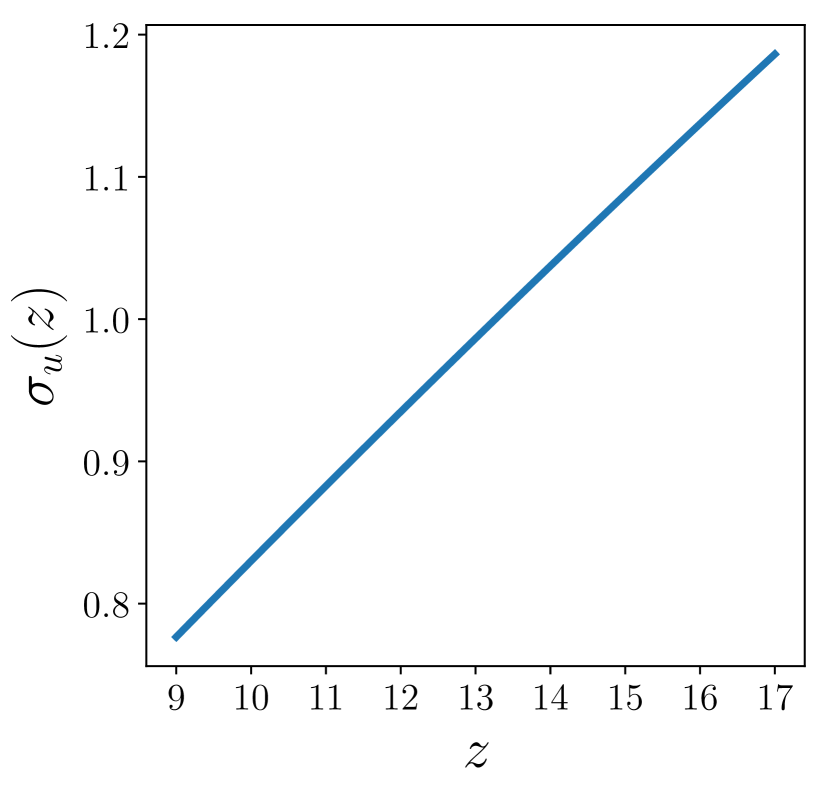
(a) Variance $\sigma_{u}$ is an increasing function of $z$ for the considered normal-discrete model

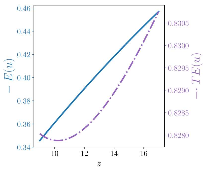
(b) $\mathrm{E}(u)$ and $TE=\mathrm{E}(e^{-u})$ in the range $10.5\leq z\leq 17$ are both monotonically increasing function of $z$ and thus of $\sigma_{u}$

Figure 1: Unusual behaviour of the discrete normal model

Thus if in reality the distribution of $u$ is discrete as in (26), that is, $u$ is generated from the discrete distribution and $v$ is generated from a normal distribution so that the model is a normal-discrete model specified by (1) and (23), and one applies the normal-exponential model (1) and (2), the estimates are likely to suffer from model misspecification. Use of the normal-exponential model according to (9), (10) an increase in $z$ causes a decrease of $TI$, while the real situation is the opposite.

3.3 Discrete distribution. Mean $TE$

To illustrate the aforementioned problem we run simulations with the following specifications. We choose the sample size $N=1000$. The single input $x_{i}$ is generated from an uniform distribution defined for the interval $[2,7]$. The noise term $v_{i}\sim N(0,0.25)$. A single variable $z_{i}$ comes from an uniform distribution defined in the interval $[9,17]$. The parameters of the discrete distribution of $u$ in (23) are: $u_{i,1}=0.1$; $u_{i,2}=1+0.2z_{i}$; $p_{i}=0.9+0.001z_{i}$. To simulate $u_{i}$, we also define an uniformly distributed random variable $r_{i}\sim U[0,1]$ for each $i$. We then assign $u_{i}=u_{i,1}$ if $r_{i}<p_{i}$ and $u_{i}=u_{i,2}$ otherwise. Finally we generate output $y_{i}$ according to $y_{i}=1+x_{i}+v_{i}-u_{i}$.

Using the generated data we estimated parameters of normal-exponential model (1) and (2) with the following specification for $\sigma_{u}(z)$, viz., $\ln\sigma_{u}(z_{i})=\gamma_{0}+\gamma z_{i}$, and obtained

$$\hat{\sigma}_{u_{i}}=\exp(-0.618+0.025z_{i}).$$

We used this estimate of $\sigma_{u}(z_{i})$ to get estimate of $TE$ using (3), i.e., $\widehat{TE}_{i}={1}/({1+\hat{\sigma}_{ui}})$.

Plot of true $\sigma_{u_{i}}$ calculated using (24) and estimated $\hat{\sigma}_{u_{i}}$ on $z$ is presented in Figure 2. Similarly, plot of true $TE_{i}$ calculate using (25) and estimated $\widehat{TE}_{i}$ on $z$ is presented in Figure 3. It can be seen from the figures that while $\hat{\sigma}_{u}$ increases with $z$, like $\sigma_{u}$, true $TE$ and the estimate of $TE$ move in opposite directions. In this case the model misspecification leads to the wrong conclusion of the negative effect of $z$ on $TE$.

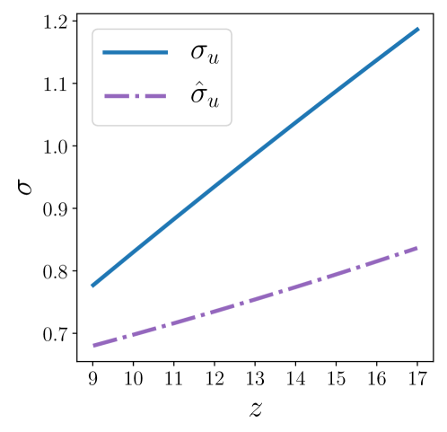
Figure 2: $\sigma_{u}$ and $\hat{\sigma}_{u}$ behave in a similar way for the normal-discrete model

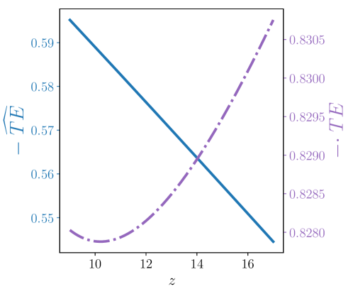
Figure 3: $TE$ and $\widehat{TE}$ as function of $z$ behave in a different way for the normal-discrete model

3.4 Discrete distribution. Observation-specific $TE$

We continue with the discrete case to provide another counter-example when $TE$ is estimated from the conditional mean. For this we consider a discrete random variable $u>0$ which takes values $u_{i}=z\,u_{i0}$, $i=1,2$ with probabilities $p_{1},p_{2}$, such that $p_{1}+p_{2}=1$, and $u_{i0}>0$, $i=1,2$, $z>0$.

$$P(u_{i}=zu_{i0})=p_{i},\,\,\,i=1,2.$$ (27)

Variance of $u_{i}$ depends on $z$, i.e.,

$$\sigma^{2}_{ui} =z^{2}p_{1}p_{2}(u_{10}-u_{20})^{2}=z^{2}c^{2},\,\,\,\,c>0,$$ (28)

where $c=p_{1}p_{2}(u_{10}-u_{20})$. Thus

$$\sigma_{u}=z\,c,\,\,\text{and}\,\,\frac{\partial\sigma_{u}}{\partial z}=c>0,$$ (29)

Statement 4.

Consider the SF model (1) with $v_{i}\sim\mathcal{N}(0,\sigma_{v}^{2})$ and a one-parameter distribution for $u$ in (27). Then the sign of the marginal effect of $z$ on $TE$ defined as $TE=E(e^{-u}|\varepsilon)$ is:

$$\frac{\partial TE}{\partial z} =\frac{\partial\mathrm{E}(e^{-u}|\varepsilon)}{\partial z}$$

$$=-\frac{1}{\sum\nolimits_{i=1}^{2}p_{i}e^{-w_{i}}}\sum\nolimits_{i=1}^{2}p_{i}e^{-z\,u_{i0}}e^{-w_{i}}(u_{i0}+w^{\prime}_{i})$$

$$+\frac{1}{\left(\sum\nolimits_{i=1}^{2}p_{i}e^{-w_{i}}\right)^{2}}\left(\sum\nolimits_{i=1}^{2}p_{i}e^{-z\,u_{i0}}e^{-w_{i}}\right)\left(\sum\nolimits_{i=1}^{2}p_{i}e^{-w_{i}}w^{\prime}_{i}\right),$$

where $w_{i}=\frac{(z\,u_{i0}+\varepsilon)^{2}}{2\sigma_{v}^{2}}$ and $w^{\prime}_{i}=\frac{\partial}{\partial z}w_{i}=\frac{z\,u_{i0}^{2}+\varepsilon\,u_{i0}}{\sigma_{v}^{2}}$.

The proof is presented in the Appendix.

Note that the marginal effect of $z$ on $TE$ in the normal-exponential model is negative if $\frac{\partial\sigma_{u}}{\partial z}>0$ (see Theorem 2). However, in the normal-discrete model, the sign of the marginal effect of $z$ depends on value of $\varepsilon$. That is, the value of the marginal effect as well its sign depends on the value of $\varepsilon$.

We illustrate this with the plot of $\frac{\partial TE}{\partial z}$ against $\varepsilon$ for these values of the model parameters: $\,z=8.5;\,\sigma_{v}=1;\,u_{1}=0.1;\,u_{2}=0.89;\,p_{1}=0.99;\,p_{2}=0.01$

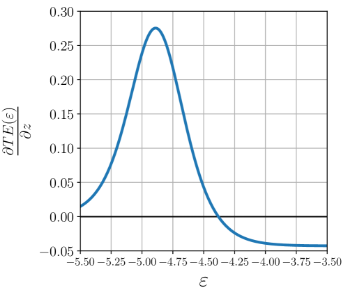
Figure 4: Marginal effect $\frac{\partial TE}{\partial z}$ as function of $\varepsilon$ for $z=8.5;\,\sigma_{v}=1;\,u_{1}=0.1;\,u_{2}=0.89;\,p_{1}=0.99;\,p_{2}=0.01$

From Figure 4 one can see that if the normal-discrete model is the true model, then the sign of the marginal effect may vary across observations. But for the normal-exponential model the marginal effect is always negative if $\frac{\partial\sigma_{u}}{\partial z}>0$. Thus if the normal-exponential model is used, where the true model is normal-discrete, one can come to the wrong conclusion regarding the sign of the marginal effect.

Sometimes the focus is not on the individual values of $TE$ but their rankings. To examine how the true values of $TE$ are related to their estimated counterparts for the simulated model, we consider the following simulations. We used $N=1000$, generated input $x_{i}$ from a uniformly distributed random variable in the interval $[2,2.3]$. The noise term is generated from $v_{i}\sim N(0,\,1)$. The $z_{i}$ variable is generated from a uniformly distributed random variable in the interval $[8,9.4]$. The parameters of the distribution of the discrete distribution of $u$ are chosen as: $p_{1}=0.8,p_{2}=0.2;u_{(1)}=0.1,u_{(2)}=0.89$. We also generated a variable $r_{i}$ which is uniformly distributed in the interval $[0,1]$. Then we generated $u_{i0}=u_{(2)}$ if $r_{i}<p_{2}$ and $u_{i0}=u_{(1)}$ otherwise, and assume $u_{i}=z_{i}\,u_{i0}$. Finally we generated output $y_{i}$ as: $y_{i}=1+x_{i}+v_{i}-u_{i}$.

We used these data to estimate the parameters of the normal-exponential model (1)–(2) with the following specification of $\sigma_{u}$: $\ln\sigma_{ui}=\gamma_{0}+\gamma z_{i}$, and obtained the estimates of the observation specific technical efficiencies $\widehat{TE}_{i}$.

For each $i$ true $\widehat{TE}_{i}$ was calculated as

$$TE_{i}=\mathrm{E}(e^{-u}|\varepsilon_{i})=\frac{\left(\sum_{i=1}^{k}p_{i}e^{-z_{i}\,u_{i}}e^{-w_{i}}\right)}{\left(\sum_{i=1}^{k}p_{i}e^{-w_{i}}\right)},$$ (30)

where $w_{i}=\frac{(z_{i}\,u_{i}+\varepsilon_{i})^{2}}{2\sigma_{v}^{2}}$.

A scatter plot of the estimated TE, $\widehat{TE}_{i}$ against true $TE_{i}$ provided in Figure 5. It can be seen that in case of positive true marginal effect $TE$ we get confusing values as estimates, while modeling capability of normal-exponential model is better if the signs of marginal effects coincide.

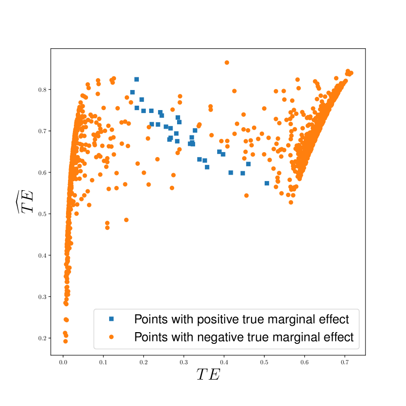
(a) Comparison of all estimates of $\widehat{TE}$ and true $TE$

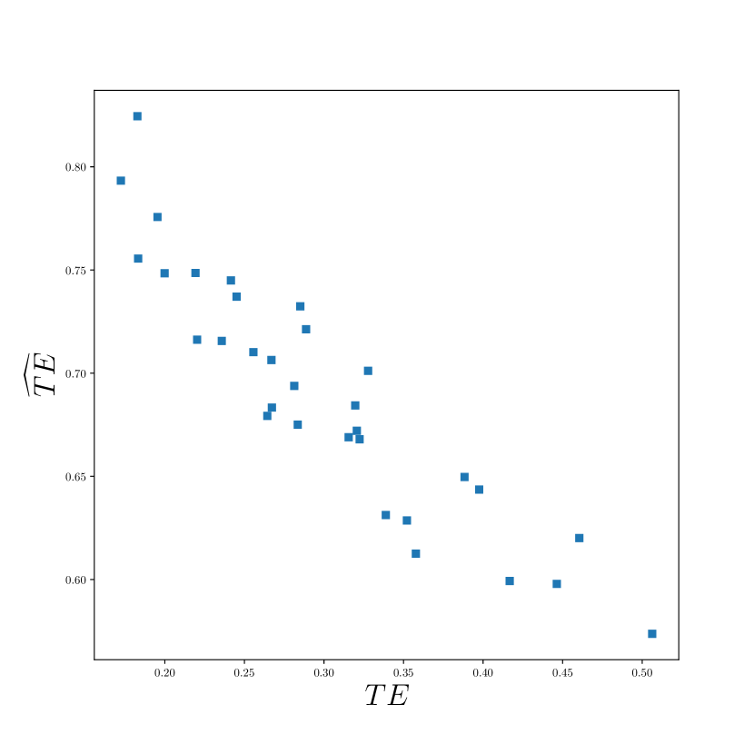
(b) Selected points with $\varepsilon$ between $-2.3$ and $-2.1$

Figure 5: Scatter plot of $\widehat{TE}$ and true $TE$

4 Conclusions and discussions

In this paper we derived the formula for computing the marginal effects of determinants of inefficiency ($z$) on both the unconditional and conditional means of technical inefficiency and efficiency for the normal-exponential stochastic frontier model. We proved that for the normal-exponential model the signs of the marginal effects of $z$ on the technical inefficiency and technical efficiency are of opposite sign.

We considered an example of discrete distribution for technical inefficiency and showed that the relationship between the true and estimated technical efficiency for the normal-discrete model can be substantially different from the normal-exponential model, at least for some values of $z$. This results illustrates that if the real world data on noise and inefficiency comes from a normal and a discrete distribution and a researcher estimates the model assuming that the errors are normal and exponential instead, results on estimated efficiency, its marginal effect and rankings might be all wrong. That is, the consequence of misspecification of inefficiency distribution can be quite serious.

Appendix A Proofs

A.1 Proof of Theorems 1 and 2

First we reproduce a proof of the Lemma 1 from (Sampford (1953)):

Lemma 1.

Let $\phi(z)$ and $\Phi(z)$ be the probability density function and the cumulative density function of the standard normal distribution $\mathcal{N}(0,1)$, and $\lambda(z)=\frac{\phi(z)}{\Phi(z)}$. Then it holds:

1. $1-z\lambda(z)-\lambda(z)^{2}\geq 0$

2. $\lambda(z)$ is a decreasing function and its derivative $\lambda^{\prime}(z)\in(-1,0)$.

Proof.

Obviously $f(t)=\frac{\phi(t)}{\Phi(z)}=\frac{\phi(t)}{P(Z\leq z)}$ is a probability density function of a random variable $X$ defined at the interval $(-\infty,z)$.

$$\mathrm{E}(X) =\int\limits_{-\infty}^{z}t\frac{\phi(t)}{\Phi(z)}dt=\frac{1}{\Phi(z)}\int\limits_{-\infty}^{z}t\phi(t)dt=-\frac{1}{\Phi(z)}\int\limits_{-\infty}^{z}\phi^{\prime}(t)dt=-\frac{\phi(z)}{\Phi(z)}=-\lambda(z),$$

$$\mathrm{E}(X^{2}) =\int\limits_{-\infty}^{z}t^{2}\frac{\phi(t)}{\Phi(z)}dt=\frac{1}{\Phi(z)}\int\limits_{-\infty}^{z}t^{2}\phi(t)dt=-\frac{1}{\Phi(z)}\int\limits_{-\infty}^{z}t\phi^{\prime}(t)dt=$$

$$=-\frac{1}{\Phi(z)}\biggl{(}\Bigl{.}t\phi(t)\Bigr{|}_{-\infty}^{z}-\int\limits_{-\infty}^{z}\phi(t)dt\biggr{)}=-\frac{1}{\Phi(z)}\bigl{(}z\phi(z)-\Phi(z)\bigr{)}=1-z\lambda(z).$$

Hence, the variance is

$$\mathrm{Var}(X)=1-z\lambda(z)-(-\lambda(z))^{2}=1-z\lambda(z)-\lambda(z)^{2}\geq 0.$$

Since

$$\lambda^{\prime}(z) =\left(\frac{\phi(z)}{\Phi(z)}\right)^{\prime}=\frac{1}{\Phi(z)^{2}}\bigl{(}\phi(z)^{\prime}\Phi(z)-\phi(z)\Phi(z)^{\prime}\bigr{)}=-z\lambda(z)-\lambda(z)^{2}$$

$$=\mathrm{Var}(X)-1,$$

we have $-1\leq\lambda^{\prime}(z)\leq 0$. ∎

A.1.1 Proof of Theorem 1

Proof.

From Statement 1 we have

$$\frac{\partial\mathrm{E}(u|\varepsilon)}{\partial\sigma_{u}} =\frac{\sigma_{v}^{2}}{\sigma_{u}^{2}}\frac{\Phi^{2}(z)-\phi^{2}(z)-z\phi(z)\Phi(z)}{\Phi^{2}(z)}=\frac{\sigma_{v}^{2}}{\sigma_{u}^{2}}\bigl{(}1-z\lambda(z)-z\lambda(z)^{2}\bigr{)},$$

which is non-negative by Lemma 1. ∎

A.1.2 Proof of Theorem 2

Proof.

From Statement 2 we have

$$\frac{\partial TE}{\partial\sigma_{u}} =\frac{\sigma_{v}}{\sigma_{u}^{2}}\cdot\frac{\exp\left(-z\sigma_{v}+\frac{\sigma_{v}^{2}}{2}\right)}{\Phi^{2}(z)}\Phi(z)\Phi(z-\sigma_{v})\bigl{(}-\sigma_{v}+\lambda(z-\sigma_{v})-\lambda(z)\bigr{)}.$$ (31)

Since the first factors in (31) and $\sigma_{v}$ are greater or equal to $0$, it is enough to prove that

$$f(t)=-t+\lambda(z-t)-\lambda(z)\leq 0\text{\, for all \,}t\geq 0.$$

We have $f(0)=0$, and $f^{\prime}(t)=-1-\lambda^{\prime}(z-t)\leq 0$ since $-1\leq\lambda(t)\leq 0$ for all $t$ (Lemma 1). Thus $f(t)\leq 0$, and Theorem 2 is proven. ∎

A.2 Proof of Theorems 3 and 4

Statement 5.

For $\lambda(z)=\frac{\phi(z)}{\Phi(z)}$ it holds that:

$$2\lambda^{2}(z)>1-z^{2}-3z\lambda(z)\text{ for }z<0.$$ (32)

Proof.

According to the proof of Theorem 9 in (Gasull and Utzet (2014)) we get that:

$$2+x^{2}a^{2}(x)-a^{2}(x)-3xa(x)>0\text{ for }x>0,$$

where

$$a(x)=\frac{1-\Phi(x)}{\phi(x)}=\frac{1}{\lambda(-x)}.$$

So,

$$2+x^{2}\frac{1}{\lambda^{2}(-x)}-\frac{1}{\lambda^{2}(-x)}-3x\frac{1}{\lambda(-x)}>0\text{ for }x>0.$$

By the change of variable $z=-x$ we get:

$$2+z^{2}\frac{1}{\lambda^{2}(z)}-\frac{1}{\lambda^{2}(z)}+3z\frac{1}{\lambda(z)}>0\text{ for }z<0.$$

Moving $\frac{1}{\lambda^{2}(z)}$ we obtain the following inequality:

$$\frac{1}{\lambda^{2}(z)}\left[2\lambda^{2}(z)+z^{2}-1+3z\lambda(z)\right]>0\text{ for }z<0.$$

As $\lambda^{2}(z)>0$, this inequality is equivalent to:

$$2\lambda^{2}(z)+z^{2}-1+3z\lambda(z)>0\text{ for }z<0.$$

Moving two terms to the right side of the inequality we get the statement:

$$2\lambda^{2}(z)>1-z^{2}-3z\lambda(z)\text{ for }z<0.$$

∎

Proof of Theorem 3

Proof.

Denote by $A=\frac{\mu_{*}}{\sigma_{*}}$. As $A$ we have:

$$A =-\varepsilon\frac{\sigma_{u}^{2}}{\sigma_{u}^{2}+\sigma_{v}^{2}}\cdot\frac{\sqrt{\sigma_{u}^{2}+\sigma_{v}^{2}}}{\sigma_{u}\sigma_{v}}=-\varepsilon\frac{\sigma_{u}}{\sigma_{v}}\frac{1}{\sqrt{\sigma_{u}^{2}+\sigma_{v}^{2}}}=$$

$$=-\varepsilon\frac{1}{\sigma_{v}^{2}}\frac{\sigma_{u}\sigma_{v}}{\sqrt{\sigma_{u}^{2}+\sigma_{v}^{2}}}=-\varepsilon\frac{\sigma_{*}}{\sigma_{v}^{2}}.$$

Using this notation we get:

$$\mathrm{E}(u|\varepsilon)=\sigma_{*}\frac{\phi(A)}{\Phi(A)}+\sigma_{*}A=\sigma_{*}\left[\frac{\phi(A)}{\Phi(A)}+A\right].$$

The desired partial derivative has the form:

$$\frac{\partial}{\partial\sigma_{*}}\mathrm{E}(u|\varepsilon)=\frac{\partial}{\partial\sigma_{*}}\left[\sigma_{*}\left(\frac{\phi(A)}{\Phi(A)}+A\right)\right]=\frac{\partial}{\partial\sigma_{*}}\left[\sigma_{*}(\lambda(A)+A)\right]=$$

$$=\lambda(A)+A+\sigma_{*}(\lambda^{\prime}(A)+1)\frac{\partial A}{\partial\sigma_{*}}=\lambda(A)+A+(1+\lambda^{\prime}(A))\sigma_{*}\left(\frac{-\varepsilon}{\sigma_{v}^{2}}\right)=$$

$$=\lambda(A)+A+(1+\lambda^{\prime}(A))A=\lambda(A)+2A+A\lambda^{\prime}(A)=$$

$$=\frac{\phi(A)\Phi(A)+2A\Phi^{2}(A)+A(-A\phi(A)\Phi(A)-\phi^{2}(A)}{\Phi^{2}(A)}=$$

$$=\frac{1}{\Phi^{2}(A)}\left(\phi(A)\Phi(A)+2A\Phi^{2}(A)-A^{2}\phi(A)\Phi(A)-A\phi^{2}(A)\right),$$

as

$$\lambda^{\prime}(z) =\frac{\partial}{\partial z}\frac{\phi(z)}{\Phi(z)}=\frac{\phi^{\prime}(z)\Phi(z)-\phi(z)\Phi^{\prime}(z)}{\Phi^{2}(z)}=\frac{-z\phi(z)\Phi(z)-\phi^{2}(z)}{\Phi^{2}(z)}$$

$$=-z\lambda(z)-\lambda^{2}(z),$$

and

$$\frac{\partial A}{\partial\sigma_{*}}=\frac{\partial}{\partial\sigma_{*}}\left(-\varepsilon\frac{\sigma_{*}}{\sigma_{v}^{2}}\right)=-\frac{\varepsilon}{\sigma_{v}^{2}}.$$

So, to prove the theorem it is sufficient to prove that

$$\forall z,\,\psi(z)=\phi(z)\Phi(z)+2z\Phi^{2}(z)-z^{2}\phi(z)\Phi(z)-z\phi^{2}(z)>0.$$

It is equivalent to

$$\lambda(z)+2z-z^{2}\lambda(z)-z\lambda^{2}(z)>0.$$ (33)

We start with the case $z<0$.

Multiplying the inequality by $2$ we get an equivalent inequality:

$$2\lambda(z)+4z-2z^{2}\lambda(z)-2z\lambda^{2}(z)>0.$$

From (32) in Statement 5 above:

$$2\lambda(z) +4z-2z^{2}\lambda(z)-2z\lambda^{2}(z)>2\lambda(z)+4z-2z^{2}\lambda(z)-z\left(1-z^{2}-3z\lambda(z)\right)$$

$$=2\lambda(z)+4z-2z^{2}\lambda(z)-z+z^{3}+3z^{2}\lambda(z)$$

$$=2\lambda(z)+3z+z^{2}\lambda(z)+z^{3}=(2+z^{2})\lambda(z)+3z+z^{3}.$$

So, it is sufficient to prove, that for $z<0$:

$$(2+z^{2})\lambda(z)+3z+z^{3}>0.$$ (34)

From (Baricz (2008)) we get that the following inequality holds:

$$\frac{1}{\lambda(-x)}<\frac{4}{\sqrt{x^{2}+8}+3x},x>0.$$

Using the change of variables $z=-x$ we get:

$$\frac{1}{\lambda(z)}<\frac{4}{\sqrt{z^{2}+8}-3z},z\leq 0.$$

The exchange of nominator and denominator leads to:

$$\lambda(z)>\frac{1}{4}\left(\sqrt{z^{2}+8}-3z\right),z\leq 0.$$ (35)

The inequality (34) is equivalent to:

$$\lambda(z)>\frac{-3z-z^{3}}{2+z^{2}}.$$

So, using the bound (35) it is sufficient to prove, that for $z<0$:

$$\frac{1}{4}\left(\sqrt{z^{2}+8}-3z\right)>\frac{-3z-z^{3}}{2+z^{2}}.$$

For $x=-z\geq 0$ we get an equivalent inequality:

$$\frac{1}{4}\left(\sqrt{x^{2}+8}+3x\right)>\frac{3x+x^{3}}{2+x^{2}}.$$

Rearranging the terms we get the inequality:

$$\sqrt{x^{2}+8}>4\frac{3x+x^{3}}{2+x^{2}}-3x.$$ (36)

For the right side we have:

$$4\frac{3x+x^{3}}{2+x^{2}}-3x=\frac{12x+4x^{3}-3x^{3}-6x}{2+x^{2}}=\frac{x^{3}+6x}{2+x^{2}}=x+\frac{4x}{x^{2}+2}.$$

Both parts of (36) are positive, so (36) is equivalent to:

$$x^{2}+8>\left(x+\frac{4x}{x^{2}+2}\right)^{2}.$$

Moving $x^{2}$ to the right side we get:

$$8>\frac{8x^{2}}{x^{2}+2}+\frac{16x^{2}}{(x^{2}+2)^{2}}.$$

Moving the first term at the right side to the left we get:

$$8\left(1-\frac{x^{2}}{x^{2}+2}\right)>\frac{16x^{2}}{(x^{2}+2)^{2}}.$$

Subtracting $\frac{x^{2}}{x^{2}+2}$ from $1$ we obtain:

$$8\frac{2}{x^{2}+2}>\frac{16x^{2}}{(x^{2}+2)^{2}}.$$

As

$$1>\frac{x^{2}}{x^{2}+2}.$$

we proved (33) for $z<0$. The remaining part is the proof of (33) for $z>0$.

As

$$-1\leq\lambda^{\prime}(z)\leq 0,$$

we have:

$$\lambda(z)+2z-z^{2}\lambda(z)-z\lambda^{2}(z)=\lambda(z)+2z+z\lambda^{\prime}(z)\geq\lambda(z)+2z+(-z)=\lambda(z)+z>0.$$

QED. ∎

A.2.1 Proof of Theorem 4

Proof.

$$\mathrm{E}(e^{-u}|\varepsilon)=\frac{\Phi\left(\frac{\mu_{*}}{\sigma_{*}}-\sigma_{*}\right)}{\Phi\left(\frac{\mu_{*}}{\sigma_{*}}\right)}e^{-\mu_{*}+\frac{1}{2}\sigma_{*}^{2}}.$$

For $A$ we have

$$A=\frac{\mu_{*}}{\sigma_{*}}=-\varepsilon\frac{\sigma_{*}}{\sigma_{v}^{2}}.$$

Then the partial derivative with respect to $\sigma_{*}$ has the form:

$$\frac{\partial A}{\partial\sigma_{*}}=-\frac{\varepsilon}{\sigma_{v}^{2}}.$$

For $E(e^{-u}|\varepsilon)$ we obtain:

$$\mathrm{E}(e^{-u}|\varepsilon)=\frac{\Phi(A-\sigma_{*})}{\Phi(A)}e^{-A\sigma_{*}+\frac{1}{2}\sigma_{*}^{2}}.$$

Then the partial derivative has the form:

$$\frac{\partial\mathrm{E}(e^{-u}|\varepsilon)}{\partial\sigma_{*}} =\frac{\partial}{\partial\sigma_{*}}\left[\frac{\Phi(A-\sigma_{*})}{\Phi(A)}\right]e^{-A\sigma_{*}+\frac{1}{2}\sigma_{*}^{2}}$$

$$+\frac{\Phi(A-\sigma_{*})}{\Phi(A)}e^{-A\sigma_{*}+\frac{1}{2}\sigma_{*}^{2}}\frac{\partial}{\partial\sigma_{*}}\left(-A\sigma_{*}+\frac{1}{2}\sigma_{*}^{2}\right).$$

We continue to expand the terms above using in addition the following:

$$-A\sigma_{*}+\frac{1}{2}\sigma_{*}^{2}=\frac{\varepsilon\sigma_{*}^{2}}{\sigma_{v}^{2}}+\frac{1}{2}\sigma_{*}^{2}=\sigma_{*}^{2}\left(\frac{1}{2}+\frac{\varepsilon}{\sigma_{v}^{2}}\right).$$

So,

$$\frac{\partial\mathrm{E}(e^{-u}|\varepsilon)}{\partial\sigma_{*}} =\frac{1}{\Phi^{2}(A)}\Biggl{(}\phi(A-\sigma_{*})\left(-\frac{\varepsilon}{\sigma_{v}^{2}}-1\right)\Phi(A)$$

$$-\Phi(A-\sigma_{*})\phi(A)\left(-\frac{\varepsilon}{\sigma_{v}^{2}}\right)\Biggr{)}e^{-A\sigma_{*}+\frac{1}{2}\sigma_{*}^{2}}+$$

$$+\frac{\Phi(A-\sigma_{*})}{\Phi(A)}e^{\sigma_{*}^{2}\left(\frac{1}{2}+\frac{\varepsilon}{\sigma_{v}^{2}}\right)}2\sigma_{*}\left(\frac{1}{2}+\frac{\varepsilon}{\sigma_{v}^{2}}\right)=$$

$$=\frac{\Phi(A-\sigma_{*})}{\Phi(A)}e^{\sigma_{*}^{2}\left(\frac{1}{2}+\frac{\varepsilon}{\sigma_{v}^{2}}\right)}\frac{1}{\sigma_{*}}\sigma_{*}\Bigg{(}\lambda(A-\sigma_{*})\left(-\frac{\varepsilon}{\sigma_{*}^{2}}-1\right)-$$

$$-\lambda(A)\left(-\frac{\varepsilon}{\sigma_{v}^{2}}\right)+2\sigma_{*}\left(\frac{1}{2}+\frac{\varepsilon}{\sigma_{v}^{2}}\right)\Bigg{)}.$$

So, we need to prove that:

$$\sigma_{*}\left(\lambda(A-\sigma_{*})\left(-\frac{\varepsilon}{\sigma_{*}^{2}}-1\right)-\lambda(A)\left(-\frac{\varepsilon}{\sigma_{v}^{2}}\right)+2\sigma_{*}\left(\frac{1}{2}+\frac{\varepsilon}{\sigma_{v}^{2}}\right)\right)<0.$$

Or equivalently:

$$\lambda(A-\sigma_{*})(A-\sigma_{*})-\lambda(A)A+\sigma_{*}^{2}-2A\sigma_{*}<0.$$

If $x=A-\sigma_{*}$, then $A=x+\sigma_{*}=x+t,t>0$ and we have:

$$\lambda(x)x-\lambda(x+t)(x+t)+t^{2}-2(x+t)t<0$$

Opening brackets we get:

$$\lambda(x)x-\lambda(x+t)(x+t)-t^{2}-2xt<0$$

So, we need to prove that for $t>0$ and arbitrary $x$:

$$\psi(x,t)=(x+t)\lambda(x+t)-x\lambda(x)+t^{2}+2xt>0.$$

It holds that $\psi(x,0)=0$. Then it is sufficient to prove that the function is increasing i.e. the corresponding partial derivative is positive:

$$\frac{\partial\psi(x,t)}{\partial t}=\lambda(x+t)+(x+t)\lambda^{\prime}(x+t)+2t+2x>0.$$

Using the change of variables $z=x+t$ we get the inequality for $z\in(-\infty,+\infty)$:

$$\lambda(z)+z\lambda^{\prime}(z)+2z>0.$$

For $z>0$ it is obvious that:

$$z(1+\lambda^{\prime}(z))+(z+\lambda(z))>0,$$

as $0<1+\lambda^{\prime}(z)<1$ and $z+\lambda(z)>0$.

For $z<0$ it is more complicated. We need to prove, that for $z<0$

$$\lambda(z)+2z-z^{2}\lambda(z)-z\lambda^{2}(z)>0.$$

Substituting $\lambda(z)$ by $\frac{\phi(z)}{\Phi(z)}$ we get:

$$\phi(z)\Phi(z)+2z\Phi^{2}(z)-z^{2}\phi(z)\phi(z)-z\phi^{2}(z)>0.$$

We apply the change of variables $x=-z$, so for $x>0$ we want to prove:

$$\phi(x)\Phi(-x)-2x\Phi^{2}(-x)-x^{2}\phi(x)\Phi(-x)+x\phi^{2}(x)>0.$$

Let $F(x)=\Phi(-x)$. Then we need to prove for $x>0$:

$$\phi(x)F(x)+2xF^{2}(x)-x^{2}\phi(x)F(x)+x\phi^{2}(x)>0.$$

Rearranging terms we get the inequality:

$$(1-x^{2})\phi(x)F(x)+x\phi(x)^{2}-2xF(x)^{2}>0\text{ for }x>0,$$ (37)

where $F(x)=1-\Phi(x)$. To prove it we’ll split the whole interval $(0,\infty)$ into two smaller ones: $(0,1]$ and $(1,\infty)$.

$x\in(1,\infty)$

In this case $1-x^{2}<0$, and to prove (37) it is sufficient to prove:

$$(1-x^{2})\frac{4}{\sqrt{x^{2}+8}+3x}+x-2x\frac{16}{(\sqrt{x^{2}+8}+3x)^{2}}>0,$$

as it holds that $F(x)\leq\frac{4}{\sqrt{x^{2}+8}+3x}\phi(x)$ according to (Baricz, 2007).

Then by multiplying by $(\sqrt{x^{2}+8}+3x)^{2}$ we get:

$$4(1-x^{2})(\sqrt{x^{2}+8}+3x)+x(\sqrt{x^{2}+8}+3x)^{2}-32x$$

$$=4\sqrt{x^{2}+8}+12x-4x^{2}\sqrt{x^{2}+8}-12x^{3}-32x$$

$$\qquad+x(x^{2}+8+9x^{2}+6x\sqrt{x^{2}+8})$$

$$=4\sqrt{x^{2}+8}-4x^{2}\sqrt{x^{2}+8}-20x-12x^{3}+10x^{3}+8x+6x^{2}\sqrt{x^{2}+8}$$

$$=4\sqrt{x^{2}+8}+2x^{2}\sqrt{x^{2}+8}-12x-2x^{3}.$$

So, we need to prove that:

$$4\sqrt{x^{2}+8}+2x^{2}\sqrt{x^{2}+8}>12x+2x^{3}\Leftrightarrow$$

$$\sqrt{x^{2}+8}(2+x^{2})>6x+x^{3}.$$

As the left side and the right side of inequality are positive for $x>0$ it is equivalent to the inequalities for the squares of both sides:

$$(x^{2}+8)(2+x^{2})^{2}>(6x+x^{3})^{2}\Leftrightarrow$$

$$(x^{2}+8)(4+4x^{2}+x^{4})>36x^{2}+12x^{4}+x^{6}\Leftrightarrow$$

$$4x^{2}+4x^{4}+x^{6}+32+32x^{2}+8x^{4}>36x^{2}+12x^{4}+x^{6}\Leftrightarrow$$

$$32+36x^{2}+12x^{4}+x^{6}>36x^{2}+12x^{4}+x^{6}\Leftrightarrow$$

$$32>0.$$

We proved the inequality for the case $x>1$.

Value of $x$ between $0$ and $1$

We use the following strategy: we split to smaller intervals, for each interval we provide a bound $\phi(x)>cF(x)$ defined by the left edge of the interval as $\left(\phi(x)/F(x)\right)^{\prime}>0$ according to Lemma 1, and then get a quadratic inequality or a linear inequality, which is easy to check.

Let’s start with $x\in(0.9,1]$. $\phi(x)>1.44F(x)$, then

$$(1-x^{2})\phi(x)F(x)+x\phi(x)^{2}-2xF^{2}(x)>$$

$$(1-x^{2})1.44F^{2}(x)+2.07xF^{2}(x)-2xF^{2}(x)\geq$$

$$2.07xF^{2}(x)-2xF^{2}(x)>0.07xF^{2}(x)>0.$$

We proceed in a similar way for other intervals. If $x\in(0.83,0.9]$, then $\phi(x)>1.39F(x)$. Then

$$(1-x^{2})\phi(x)F(x)+x\phi(x)^{2}-2xF(x)^{2}$$

$$\qquad>1.39(1-x^{2})F(x)^{2}+1.93xF(x)^{2}-2xF(x)^{2}\geq 0.$$

If $x\in(0.65,0.83]$, then $\phi(x)>1.25F(x)$. Then

$$(1-x^{2})\phi(x)F(x)+x\phi(x)^{2}-2xF(x)^{2}$$

$$\qquad>1.25(1-x^{2})F(x)^{2}+1.5625xF(x)^{2}-2xF(x)^{2}\geq 0.$$

If $x\in(0.4,0.65]$, then $\phi(x)>1.05F(x)$. Then

$$(1-x^{2})\phi(x)F(x)+x\phi(x)^{2}-2xF(x)^{2}$$

$$\qquad>1.05(1-x^{2})F(x)^{2}+1.1025xF(x)^{2}-2xF(x)^{2}\geq 0.$$

If $x\in[0,0.4]$, then $\phi(x)>0.75F(x)$. Then

$$(1-x^{2})\phi(x)F(x)+x\phi(x)^{2}-2xF(x)^{2}$$

$$\qquad>0.75(1-x^{2})F(x)^{2}+0.5625xF(x)^{2}-2xF(x)^{2}\geq 0.$$

QED. ∎

A.3 Proof of the Statement 4

Proof.

We consider a discrete random variable $u$. It takes values $u_{i}=z\,u_{i0},\,i=1,2$ with probabilities $p_{1},p_{2}$ correspondingly, where $u_{i0}>0,\,i=1,2$. Since $v\sim\mathcal{N}(0,\sigma_{v}^{2})$ and $u$ are independent and $\varepsilon=v-u$, the joint distribution of $u,\varepsilon$ has the form

$$f(u=u_{i},\varepsilon)=p_{i}\frac{1}{\sqrt{2\pi}\sigma_{v}}\exp\left(-\frac{(u_{i}+\varepsilon)^{2}}{2\sigma_{v}^{2}}\right).$$

Thus, the marginal pdf of $\varepsilon$ has the form:

$$f(\varepsilon)=\sum_{i=1}^{2}p_{i}\frac{1}{\sqrt{2\pi}\sigma_{v}}\exp\left(-\frac{(u_{i}+\varepsilon)^{2}}{2\sigma_{v}^{2}}\right).$$ (38)

The conditional distribution has the form:

$$P(u=u_{i}|\varepsilon)=\frac{p_{i}\frac{1}{\sqrt{2\pi}\sigma_{v}}\exp\left(-\frac{(u_{i}+\varepsilon)^{2}}{2\sigma_{v}^{2}}\right)}{\sum_{i=1}^{2}p_{i}\frac{1}{\sqrt{2\pi}\sigma_{v}}\exp\left(-\frac{(u_{i}+\varepsilon)^{2}}{2\sigma_{v}^{2}}\right)}=\frac{p_{i}e^{-w_{i}}}{p_{1}e^{-w_{1}}+p_{2}e^{-w_{2}}},\,\,\,i=1,2,$$

where $w_{i}=\frac{(u_{i}+\varepsilon)^{2}}{2\sigma_{v}^{2}}=\frac{(z\,u_{i0}+\varepsilon)^{2}}{2\sigma_{v}^{2}}$.

Then observation-specific technical efficiency is

$$TE =\mathrm{E}\left(e^{-u}|\varepsilon\right)=\sum_{i=1}^{2}{e^{-u_{i}}\frac{p_{i}e^{-w_{i}}}{\sum_{j=1}^{2}p_{j}e^{-w_{j}}}}=\frac{\sum_{i=1}^{2}p_{i}e^{-u_{i}}e^{-w_{i}}}{\sum_{j=1}^{2}p_{j}e^{-w_{j}}}$$

$$=\frac{\sum_{i=1}^{2}p_{i}e^{-z\,u_{i0}}e^{-w_{i}}}{\sum_{j=1}^{2}p_{j}e^{-w_{j}}}.$$ (39)

Then the marginal effect $\frac{\partial TE}{\partial z}$ equals:

$$\frac{\partial TE}{\partial z} =\frac{1}{\sum_{j=1}^{2}p_{j}e^{-w_{j}}}\frac{\partial}{\partial z}\sum\nolimits_{i=1}^{2}p_{i}e^{-z\,u_{i0}}e^{-w_{i}}$$

$$-\frac{1}{\left(\sum_{j=1}^{2}p_{j}e^{-w_{j}}\right)^{2}}\left(\sum\nolimits_{i=1}^{2}p_{i}e^{-z\,u_{i0}}e^{-w_{i}}\right)\frac{\partial}{\partial z}\sum\nolimits_{j=1}^{2}p_{j}e^{-w_{j}}$$

$$=-\frac{1}{\sum_{j=1}^{2}p_{j}e^{-w_{j}}}\sum\nolimits_{i=1}^{2}p_{i}e^{-z\,u_{i0}}e^{-w_{i}}(u_{i0}+w^{\prime}_{i})$$

$$+\frac{1}{\left(\sum_{j=1}^{2}p_{j}e^{-w_{j}}\right)^{2}}\left(\sum\nolimits_{i=1}^{2}p_{i}e^{-z\,u_{i0}}e^{-w_{i}}\right)\left(\sum\nolimits_{j=1}^{2}p_{j}e^{-w_{j}}w^{\prime}_{j}\right),$$

where $w^{\prime}_{i}=\frac{\partial}{\partial z}w_{i}=\frac{z\,u_{i0}^{2}+\varepsilon\,u_{i0}}{\sigma_{v}^{2}}$ ∎

Appendix B Identifiability of the normal-discrete model

We examined the discrete model in a number of ways. The most important issue to check was identifiability of the model.

We use the dataset of size $1000$, generated with the normal-discrete model, which we used for Fig.5 in Section 3. We use the maximum likelihood approach with p.d.f. from (38) to estimate the normal-discrete model. Estimated $\widehat{TE}_{i}$ for this model were calculated from (39). Also for this data we estimated two misspecified models: normal-half normal and normal-exponential and derived predicted technical efficiencies $\widehat{TE}_{i}$ for these models. Figures 6 contain comparison of true values of $TE$ and their three estimates $\widehat{TE}_{i}$ using three different models. We see that if the model is correctly specified, obtained estimates are close to the real ones. While, if we start to use common, but misspecified normal-half-normal and normal-exponential models, the estimates are worse.

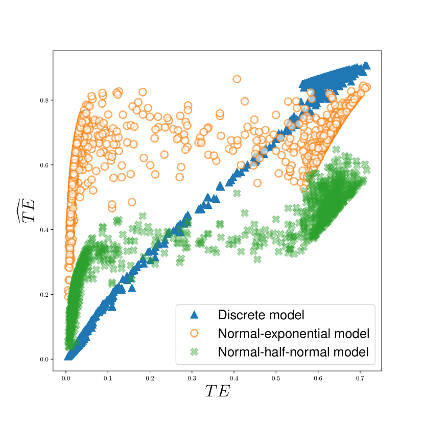
(a) Comparison of all estimates of $\widehat{TE}$ and true $TE$

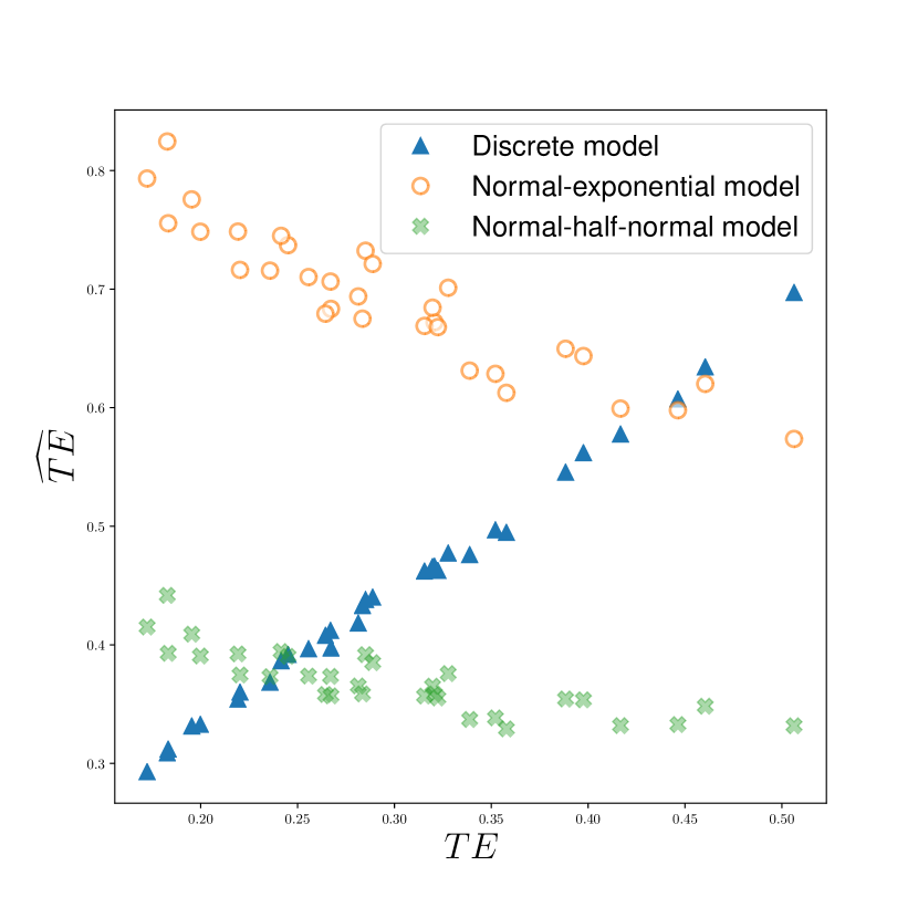
(b) Selected points with $\varepsilon$ between $-2.3$ and $-2.1$

Figure 6: Comparison of estimates $\widehat{TE}$ using a normal-discrete, a normal-half-normal and a normal-exponential models and true $TE$ obtained using a normal-discrete model

Model	Correlation	Correlation
		$-2.3<\varepsilon<-2.1$
Normal-discrete	$0.9816$	$\phantom{-}0.9971$
Normal-half-normal	$0.9451$	$-0.8768$
Normal-exponential	$0.7616$	$-0.9285$

Table 1: Spearman rank correlations for true values and the three estimates of $TE$ if the true model is normal-discrete

Spearman rank correlation between true $TE$ and the three predicted $\widehat{TE}$ are provided in Table 1. The highest rank correlation is obtained when the true model is estimated. The correlation is smaller for the for the normal-half-normal model and is even worse for the normal-exponential model. But for the subset of observations selected by the condition $-2.3<\varepsilon<-2.1$ both misspecified models provide strongly negative rank correlations of predicted $\widehat{TE}$ and true values of the technical efficiency $TE$.

References

References

- Aigner et al. (1977) Aigner, D., Lovell, C. K., and Schmidt, P. (1977). Formulation and estimation of stochastic frontier production function models. Journal of econometrics, 6(1):21–37.
- Andor and Parmeter (2017) Andor, M. and Parmeter, C. (2017). Pseudolikelihood estimation of the stochastic frontier model. Applied Economics, 49(55):5651–5661.
- Andor et al. (2019) Andor, M. A., Parmeter, C., and Sommer, S. (2019). Combining uncertainty with uncertainty to get certainty? efficiency analysis for regulation purposes. European Journal of Operational Research, 274(1):240–252.
- Baricz (2008) Baricz, Á. (2008). Mills’ ratio: monotonicity patterns and functional inequalities. Journal of Mathematical Analysis and Applications, 340(2):1362–1370.
- Battese and Coelli (1988) Battese, G. E. and Coelli, T. J. (1988). Prediction of firm-level technical efficiencies with a generalized frontier production function and panel data. Journal of econometrics, 38(3):387–399.
- Battese and Coelli (1992) Battese, G. E. and Coelli, T. J. (1992). Frontier production functions, technical efficiency and panel data: with application to paddy farmers in india. Journal of productivity analysis, 3(1-2):153–169.
- Gasull and Utzet (2014) Gasull, A. and Utzet, F. (2014). Approximating Mill’s ratio. Journal of Mathematical Analysis and Applications, 420(2):1832–1853.
- Giannakas et al. (2003) Giannakas, K., Tran, K. C., and Tzouvelekas, V. (2003). Predicting technical efficiency in stochastic production frontier models in the presence of misspecification: a Monte-Carlo analysis. Applied Economics, 35(2):153–161.
- Jondrow et al. (1982) Jondrow, J., Lovell, C. K., Materov, I. S., and Schmidt, P. (1982). On the estimation of technical inefficiency in the stochastic frontier production function model. Journal of econometrics, 19(2-3):233–238.
- Kumbhakar and Lovell (2000) Kumbhakar, S. C. and Lovell, C. K. (2000). Stochastic frontier analysis. Cambridge university press.
- Kumbhakar and Sun (2013) Kumbhakar, S. C. and Sun, K. (2013). Derivation of marginal effects of determinants of technical inefficiency. Economics Letters, 120(2):249–253.
- Lai and Kumbhakar (2019) Lai, H. and Kumbhakar, S. C. (2019). Technical and allocative efficiency in a panel stochastic production frontier system model. European Journal of Operational Research, 278(1):255–265.
- Meeusen and van den Broeck (1977) Meeusen, W. and van den Broeck, J. (1977). Efficiency estimation from Cobb-Douglas production functions with composed error. International economic review, pages 435–444.
- Ondrich and Ruggiero (2001) Ondrich, J. and Ruggiero, J. (2001). Efficiency measurement in the stochastic frontier model. European Journal of Operational Research, 129(2):434–442.
- Ray et al. (2015) Ray, S. C., Kumbhakar, S. C., and Dua, P. (2015). Benchmarking for Performance Evaluation. Springer.
- Ruggiero (1999) Ruggiero, J. (1999). Efficiency estimation and error decomposition in the stochastic frontier model: A monte carlo analysis. European journal of operational research, 115(3):555–563.
- Sampford (1953) Sampford, M. R. (1953). Some inequalities on Mill’s ratio and related functions. The Annals of Mathematical Statistics, 24(1):130–132.
- Wang (2002) Wang, H. (2002). Heteroscedasticity and non-monotonic efficiency effects of a stochastic frontier model. Journal of Productivity Analysis, 18:241–253.
- Wang (2003) Wang, H. (2003). A stochastic frontier analysis of financing constraints on investment: the case of financial liberalization in Taiwan. Journal of Business & Economic Statistics, 21:406–419.
- Yu (1998) Yu, C. (1998). The effects of exogenous variables in efficiency measurement—a monte carlo study. European Journal of Operational Research, 105(3):569–580.