CORSIKA 8 – Towards a modern framework for the simulation of extensive air showers

Abstract

Current and future challenges in astroparticle physics require novel simulation tools to achieve higher precision and more flexibility. For three decades the FORTRAN version of CORSIKA served the community in an excellent way. However, the effort to maintain and further develop this complex package is getting increasingly difficult. To overcome existing limitations, and designed as a very open platform for all particle cascade simulations in astroparticle physics, we are developing CORSIKA 8 based on modern C++ and Python concepts. Here, we give a brief status report of the project.

1 Introduction

CORSIKA Capdevielle:1992qw ; Heck:1998vt is the most widely used, actively maintained code for Monte Carlo air shower simulation currently available. In spite of its development having started almost 30 years ago Gils:1989vi , it is still frequently extended and improved, with major updates released roughly once per year consisting mostly of improvements in the various interaction models shipped with CORSIKA. Completely new features, however, are developed only rarely nowadays, also due to the complexity of the code posing a major obstacle to their implementation: Originally written and optimized to be used only in simulations for the KASCADE experiment Klages:1996zb , and therefore designed to meet the corresponding requirements, it was not intended to serve as the general purpose tool into which it has evolved. Its monolithic structure makes modifications or extensions of the code very difficult. Besides that, CORSIKA is written in FORTRAN 77, which can no longer be considered the lingua franca within the domains of high energy and astroparticle physics, and suffers from a number of restrictions, e.g. the lack of dynamic memory or object orientation, and is therefore unattractive to learn, causing a lack of qualified and motivated contributors.

Although the C++ add-ons COAST Ulrich:2006 or recently dynstack Baack:2016 help to remedy parts of these issues to a certain degree, there are still many wishes by users for extensions that simply cannot be accommodated for with reasonable effort. It is clearly a disadvantage to wrap modern extensions around the existing "dinosource" Zwart:2018 code in comparison to fundamentally re-designing the whole framework in a consistent way.

For that reason, we reached the decision that the time has come to start a project to develop a next-generation code, with the focus on the aspects modularity, flexibility, ease of use and extensibility, efficiency, and reliability from the beginning. Of course, a key element of the new project is to keep the expertise gained and include all the lessons learned from the last decades. While the name is chosen to abide, the distinction between the legacy and next-generation CORSIKA is made through the version number, initially CORSIKA 8 for the latter. We consider CORSIKA 8 to be more of a framework for simulating particle cascades rather than an air-shower-only tool, therefore extending the applicability to wider domains of research.

To a large extent, our goals and plans are outlined in ref. Engel:2018akg and their implementation is currently ongoing work. Here, we present an overview of the most important aspects of the design.

2 Building blocks

CORSIKA 8 is developed using modern C++ accompanied by Python tools. The main building blocks of CORSIKA 8 are displayed in fig. 1 together with their relations to each other.

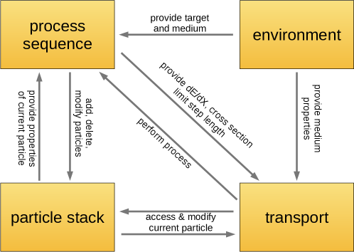
Figure 1: Main building blocks of CORSIKA 8. The relationships and dependencies between the blocks are shown as arrows. Each of these major blocks is by itself a modular system of algorithms. Basically all functionality can be replaced by alternative modules/implementations in a very straightforward way. This also means future extensions can be included easily.

2.1 Particle stack

The particle stack contains the particles in memory which are currently in the course of being propagated. In its most basic incarnation the stack provides access to the particles’ four-momenta, four-positions, and particle codes, but an easy extension of additional properties like statistical weight, as necessary e.g. for thinning algorithms, is straightforward. It is envisaged to provide optional access to the history of the particle offering a much deeper insight into its "ancestor" generations than it is currently possible with the corresponding feature Heck:2009zza of legacy CORSIKA. The particle stack is read from and written to by the process sequence, as well as the transport procedure.

2.2 Process sequence

The process sequence represents the physical processes modeled in the simulation and is composed of all the physics modules which the user chooses to enable (e.g. hadronic and electromagnetic interaction models, emission of Cherenkov light or radio). All these modules must conform to the same interfaces and are treated on the same level. We distinguish mainly between continuous processes and discrete processes (see fig. 2). While the first ones are meant to model effects which happen along the trajectory between two steps of the particle (like energy losses or Cherenkov light emission), the second type of processes typically represents interactions and decays. Furthermore, a special class of processes is reserved for the cases in which a particle transits the boundary between two media.

Discrete processes need to provide interaction lengths or decay times as a function of the particle currently being propagated (implicitly having access to information about the local environment of the particle through its location). In addition, in case one of the discrete processes is then chosen to be in fact performed, that specific process can then modify the particle stack, typically by deleting the projectile from the stack and placing new secondaries of the interaction onto the stack.

Instead of providing an interaction length, continuous processes are individually required to provide a maximum step-size. This is useful, inter alia, to limit energy losses to a tolerable amount between two steps, which would otherwise invalidate the interaction length calculated previously using the particle energy at the beginning of the step. Continuous processes are provided with the current particle together with the trajectory up to its endpoint determined from a number of criteria (see below) including the above-mentioned limited step-size. In contrast to the random nature of discrete processes, they are always performed.

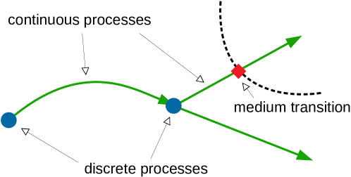
Figure 2: Discrete (blue dots) and continuous (green lines) processes during particle transport. The sampled random locations of discrete processes, which can be interactions, decays or boundary crossings (red square), determine the regime for continuous processes.

2.3 Environment

One of the most prominent features of CORSIKA 8 is the flexible definition of the medium and its properties in which the particles propagate. In particular, it will be possible to simulate not only pure air showers but also showers penetrating the ground and propagating further through ice, water, rock, or other media. A key premise of this endeavour is the ability to compose the environment out of several different (sub-)volumina with different physical properties. In this regard, CORSIKA 8 follows similar concepts as the well-known Geant4 toolkit Agostinelli:2002hh ; Allison:2006ve ; Allison:2016lfl , with the major difference perhaps being that we do not limit ourselves to homogeneous media.

Figure 3 illustrates this idea together with a sketch of the current implementation. We provide very simple volumina, in the beginning only spheres and cuboids, which the user has to furnish with models of its physical properties (in the figure symbolized by the different colors) and then assemble them into the volume tree. The structure of the volume tree represents geometrical containment, i.e., volumes fully contained by a bigger volume are child nodes of the bigger volume. The root node is always the Universe volume which is equivalent to a sphere with infinite radius. By relaxing the condition of full containment, it is possible to cut the child volume along the boundary of its parent. Furthermore, it is necessary to treat cases of overlapping nodes specially in order to avoid ambiguities. We achieve this by having references to other volumes that are to be excluded from a given volume node, in the figure indicated by the dashed arrows. The tree structure allows relatively fast queries of which actual volume contains a given point.

As a second element of the environment, it is foreseen in the design to conveniently change and extend the number of physical properties represented in the medium model. As a first step, we provide interfaces for querying mass density, fractional elementary composition, and magnetic field only. As soon as physics modules e.g. for Cherenkov or radio emission requiring the index of refraction are added to CORSIKA 8, this additional property can then easily be included. For runs without these processes enabled, however, a definition will not be required.

2.4 Transport

At the heart of CORSIKA 8 lies the transport code which, making use of the aforementioned building blocks, propagates the particles one by one, most likely producing secondaries, until the simulation finishes – by construction as soon as no particles are left.

The first step consists of proposing a trajectory, starting at the current position of the particle and initially extending to the next point of intersection with a volume boundary. We currently restrict ourselves to linear trajectories since in that case the calculations of intersections with spheres and cuboids reduce to solving polynomial equations of at most second order. For helices, which would be a natural choice for trajectories of charged particles in slowly varying magnetic fields, already the calculation of intersections with planes requires a non-trivial numerical treatment Nievergelt:1996 .

As second step, the maximum step-size is then further limited by, depending on the environment, up to two conditions concerning the numerical accuracy of the procedure. One limit regards the accuracy of integrating the equations of motion in the magnetic field to make sure that the trajectory will not deviate too much from the true, helix-like solution. This is obviously superfluous in the absence of a magnetic field or for neutral particles. The second limit pertains to the calculation of grammage $X$ along the trajectory within the medium with a given density distribution $\varrho(\bm{x})$, i.e.

$$X=\int\limits_{\mathrm{trajectory}}\varrho(\bm{x})\,\mathrm{d}s.$$ (1)

This can be done analytically exact only for very specific density distributions, e.g. a homogeneous one. For the general case, one needs to deal with either numerical integration or approximations: a suitable approach can be to approximate the density distribution $\varrho$ in the vicinity of the starting point $\bm{x}_{0}$ of the trajectory using Taylor’s expansion, say to second order,

$$\begin{split}\varrho(\bm{x}_{0}+\delta\bm{x})&=\varrho(\bm{x}_{0})+\left(\left.\bm{\nabla}\right\rvert_{\bm{x}_{0}}\varrho\right)\cdot\delta\bm{x}\\ &+\frac{1}{2}\delta\bm{x}^{\mathrm{T}}\left.H\right\rvert_{\bm{x}_{0}}\delta\bm{x}+\mathcal{O}\left(\delta x^{3}\right),\end{split}$$ (2)

where $H$ denotes the Hesse matrix of $\varrho$ and $\delta\bm{x}$ is a small piece along the trajectory. Then, the problem reduces to the integration of a polynomial and $\delta\bm{x}$ would be limited to a certain length by requiring the estimated error of the approximation to be smaller than a given value.

The next step consists of randomly sampling the next location of the discrete processes. Decay points are sampled from an exponential distribution in length, whereas for interaction points the exponentially distributed variable is grammage. To determine the location of the interaction, grammage needs to be converted back to length. Hence, an accurate conversion between these two variables is required. Afterwards, continuous processes are performed along the trajectory up to either its endpoint given by the limiting conditions described above, or the interaction point of the closest discrete process, which will be performed subsequently.

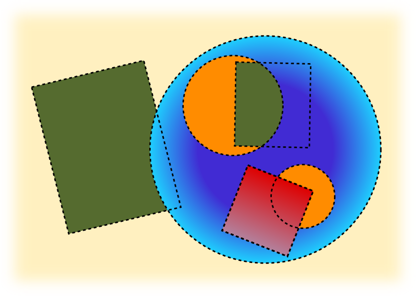
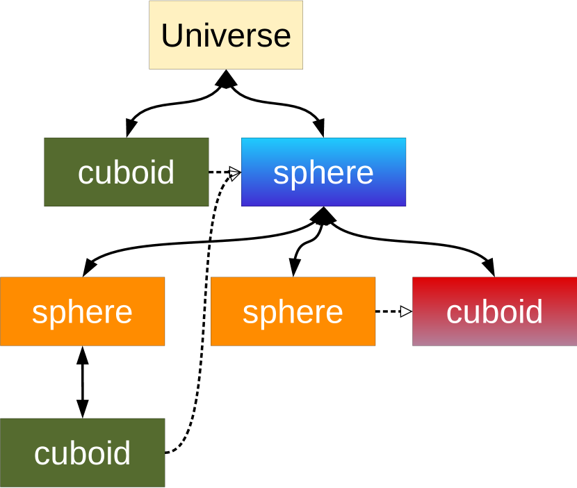
Figure 3: An example environment composed of different volumes with different physical properties indicated by color (left). In the implementation, these are assembled in a tree structure (right).

3 Conclusions and outlook

The development of CORSIKA 8 is in a very active stage. The project is completely open to input from the community. Any participation and collaboration will lead to a better tool for astroparticle physics for the next decades.

We are committed to provide a reliable, stable, accurate and flexible framework. The design as a framework, in contrast to a single-purpose program, makes it clear that the range of future applications could be far beyond just simulating extensive air shower cascades. It is also up to the community to define what is needed and what is scientifically useful. The inherent complexity of particle shower development in materials requires a very careful validation of each ingredient and input model, best with dedicated data. We aim to facilitate a better understanding and study of the relationship between these fundamental ingredients and the final physics observables.

The first intermediate development snapshots of CORSIKA 8 are already available on our gitlab server gitlab and can be obtained freely from there. We welcome any comments or, even better, participation/discussion in further developing this project. It is our plan to have a first version suitable for limited and specialized physics studies available already in 2019.

References

- (1) J.N. Capdevielle et al., tech. rep. KfK-4998, Kernforschungszentrum Karlsruhe (1992), doi:10.5445/IR/270033168
- (2) D. Heck, J. Knapp, J.N. Capdevielle, G. Schatz, T. Thouw, tech. rep. FZKA-6019, Forschungszentrum Karlsruhe (1998), https://publikationen.bibliothek.kit.edu/270043064
- (3) H.J. Gils, D. Heck, J. Oehlschlaeger, G. Schatz, T. Thouw, A. Merkel, Comput. Phys. Commun. 56, 105 (1989)
- (4) H.O. Klages et al., Nucl. Phys. B Proc. Suppl. 52, 92 (1997)
- (5) R. Ulrich, COAST (2006), https://web.ikp.kit.edu/rulrich/coast.html
- (6) D. Baack, tech. rep., Technische UniversitÃt Dortmund (2016), doi:10.17877/DE290R-19158
- (7) S.P. Zwart, Science 361, 979 (2018), 1809.02600
- (8) R. Engel, D. Heck, T. Huege, T. Pierog, M. Reininghaus, F. Riehn, R. Ulrich, M. Unger, D. Veberič, Comput. Softw. Big Sci. 3, 2 (2019), 1808.08226
- (9) D. Heck, R. Engel, tech. rep. FZKA-7495, Forschungszentrum Karlsruhe (2009), https://publikationen.bibliothek.kit.edu/270078292
- (10) S. Agostinelli et al. (GEANT4 Collaboration), Nucl. Instrum. Meth. A 506, 250 (2003)
- (11) J. Allison et al., IEEE Trans. Nucl. Sci. 53, 270 (2006)
- (12) J. Allison et al., Nucl. Instrum. Meth. A 835, 186 (2016)
- (13) Y. Nievergelt, SIAM Rev. 38, 136 (1996)
- (14) https://gitlab.ikp.kit.edu