Diagonal Padé Approximant of the one-body Green’s function, a study on Hubbard rings

Abstract

Padé approximants to the many-body Green’s function can be build by rearranging terms of its perturbative expansion. The hypothesis that the best use of a finite number of terms of such an expansion is given by the subclass of diagonal Padé approximants is here tested, and largely confirmed, on a solvable model system, namely the Hubbard ring for a variety of site numbers, fillings and interaction strengths.

I Introduction

In the context of quantum field theory, perturbation theory allows to derive a formal series for the interacting one-body Green’s function in terms of the corresponding non-interacting one. In an oversimplified notation this reads

$$G=G_{0}+G_{0}vG_{0}G_{0}+G_{0}vG_{0}G_{0}vG_{0}G_{0}+...$$ (1)

where $v$ denotes the interaction between the particles. Convergence properties of this series depend on the specific Hamiltonian one starts from; for most interesting cases the series is suspected to be, however, either divergent or merely slowly convergent. A way to overcome this limit is to sum up an infinite subset of terms, which is commonly achieved by recasting the calculation of $G$ in the form of a Dyson equation:

$$G=G_{0}+G_{0}\Sigma G,$$ (2)

where $\Sigma$, the so called self-energy of the system, has itself a (simpler) perturbative expansion in terms of $G_{0}$ and $v$, which leads to the following expansion of the Green’s function:

$$G=(G_{0}^{-1}-vG_{0}-vG_{0}vG_{0}G_{0}-...)^{-1}.$$ (3)

A finite number of terms of the expansion of $\Sigma$ results in an infinity of terms for the corresponding approximate $G$ and it usually greatly improves over the approximation provided by (1). Such an expansion is at the heart of state-of-the-art methods used nowadays for the estimate of $G$ for real systems reining.

One way to explain this success is to interpret the approach in terms of Padé approximants bakergraves. Given a certain function $f(z)$, if we only know the first $n+1$ coefficients of its Taylor expansion $f(z)=c_{0}+c_{1}z+c_{2}z^{2}+...+c_{n}z^{n}+...$, we can approximate the function with a power series that gives rise to the same expansion, which is trivially the $n^{th}$ order truncation of the Taylor series itself, $f(z)\approx c_{0}+c_{1}z+c_{2}z^{2}+...+c_{n}z^{n}$. This is what standard perturbation theory does. Alternatively, we can use the rational function

$$\frac{a_{0}+a_{1}z+a_{2}z^{2}+...+a_{p}z^{p}}{1+b_{1}z+b_{2}z^{2}+...+b_{q}z^{q}}$$ (4)

whose coefficients are determined by the same condition, namely that (4) gives rise to the same Taylor expansion of $f(z)$ up to the $n^{th}$ order. For given $n$ this criterion identifies not just one, but a set of rational functions obtained for different values of $p$ and $q$ with the constrain $p+q=n$; these functions are called ‘Padé approximants’ of order $p$ and $q$ and denoted by $[p/q]_{f}(z)$, or, in short, $[p/q]$. The special case $p=q$ is called diagonal Padé approximant. The approximant $[n/0]$ is the truncated Taylor series itself, hence the series of Padé approximants can be considered as a way to generalise the Taylor series. For many functions, Padé approximants are found to represent better approximations than truncations of the Taylor series bender. Perhaps not surprisingly, this is particularly true when the series diverges: a divergence in the Taylor expansion of a function reflects the presence of singularities over the complex plane $z\in\mathbf{Z}$ which a power series representation is incapable to describe; a rational function, on the other hand, has singularities of its own which can be ‘tuned’ to fit those of the function to approximate. If the Green’s function was simply a function of $v$, the series generated by perturbation theory (1) would amount to its Taylor expansion, or, in terms of Padé approximants, $[n/0]$, while solving the Dyson equation with the $n^{th}$ truncation of the perturbative expansion of $\Sigma$ would represent a Padé approximant $[0/n]$ (the fact that the Green’s function in facts depends on spin/space/time variables makes the definition of Padé approximants less obvious than its Taylor expansion, as we shall later see). From this perspective, it is then natural to expect that, if the perturbative series for the actual Green’s function seems to diverge, solving the Dyson equation with a perturbative self-energy may then give rise to a sequence of approximations with better convergence properties, as it turns out to be in many cases of interest.

In fact, one can go one step farther. As mentioned, for a given order of truncation of the Taylor expansion there is a variety of Padé approximants, according to the order of the numerator and denominator. For instance, given the $4^{th}$ order one can build $[4/0]$ (the truncated Taylor expansion itself), $[0/4]$ (equivalent to take $\Sigma$ up to fourth order) but also $[1/3]$, $[2/2]$, and $[3/1]$. A priori, there is no way to know which one would provide the best approximation. A large amount of evidence from numerical experiments and various applications in physics had led, however, to conjecture that, whenever no information on the function to approximate other than its truncated Taylor expansion is given, the best approximation is most likely obtained by the diagonal approximant $[n/n]$ bakergraves. This rises the question: would the equivalent of a diagonal Padé approximant work better than (3) in approximating the Green’s function?

Obviously, such a question is too vague to admit a neat answer. ‘What are the criteria to say that an approximation is “better” than another?’, ‘what fields and interactions are we considering and what is the value of the coupling constants?’ are just examples of questions one should first clarify. Moreover, even if the question were formulated with sufficient precision, practical obstacles, such as the increasing complexity of terms of perturbation theory and the scarcity of exactly known Green’s functions to use as test bench, would set severe limits to our capability to give a definite answer. Nonetheless, it does make sense to consider the possibility that diagonal Padé approximants may be a valuable tool for developing approximations of the Green’s function of real systems, for which a very limited number of terms of the expansion (1) are computationally accessible and one wishes to make the best use of them. In this paper we report a preliminary study on such a possibility.

We here focus on the simplest, nontrivial diagonal approximant, namely $[1/1]$, and perform a systematic study on a set of models, zero-temperature Hubbard rings, that are numerically solvable, in the attempt to understand whether the diagonal Padé may offer a better approximation than (1) or (3). More specifically, in Section II, we set the theoretical framework: we first derive a general expression of such an approximant for the Green’s function in terms of the expansion of the self-energy; we then simplify that expression in the case of a two-body interaction for zero temperature Green’s function in the Lehmann representation projected on a basis; finally we explain how these formulas are modified to avoid double-counting when the starting point of the expansion $G_{0}$ is not the completely free Green’s function but comes from a mean field approximation, like Hartree or density functional theory (DFT). We therefore arrive to an expression for $[1/1]$ for the Green’s function that can be readily used for model as well as for real systems. In Section III, we perform a systematic study of this approximation on zero-temperature Hubbard rings. We compare the relative error of the approximate spectral functions arising from the three approaches: straightforward perturbation theory of eqn. (1) (G-PT, henceforth), perturbation theory applied to the Dyson equation (3) ($\Sigma-$PT) and the set of diagonal Padé approximants (dP-PT), for a variety of number of sites ($L=2,4,6,8,10$), fillings ($N=2,...,2L-2$) and strengths of interaction ($U/t=0.1,1,10$). This allows us to attempt to extrapolate the convergence properties of the three series. We then focus on the direct comparison between $\Sigma$-PT and dP-PT and, finally, we discuss the advantages of building the series on top of a mean-field approximation. Conclusions are drawn at the end.

II First order diagonal Padé approximant for Green’s functions

For a scalar function $f(z)$ with Taylor expansion $\sum_{i=0}^{\infty}c_{i}z^{i}$, the first (nontrivial) diagonal Padé approximant is the rational function (here conveniently arranged in the form of a truncated continued fraction):

$$[1/1]_{f}(z)=\frac{c_{0}}{1-z\frac{c_{1}c_{0}^{-1}}{1+z\left(c_{1}c_{0}^{-1}-c_{2}c_{1}^{-1}\right)}}$$ (5)

whose Taylor expansion correctly matches that of $f(z)$ for the first $1+1+1=3$ terms: $[1/1]_{f}(z)=c_{0}+c_{1}z+c_{2}z^{2}+...$. In order to generalize this formula to cases in which the coefficients $c_{i}$ are not just numbers, but more complex objects like matrices or functions, as the one we are interested in, we follow Section 8.2 of bakergraves. As one should expect when dealing with matrices, the generalization of (5) is not unique, due to the fact that a simple product of two scalar coefficients $c_{i}c_{j}$ can correspond to either $C_{i}C_{j}$ or $C_{j}C_{i}$ if the two matrices $C_{i}$ and $C_{j}$ do not commute. The criterion we shall adopt here is that the resulting series of approximant of the Green’s function $([0/0],\;[0/1],\;[0/2],...)$ must correspond to the series $\Sigma$-PT given by (3). This unambiguously identifies a Padé generalization of standard many-body perturbation theory. We then proceed as follows.

First, suppose $c_{i}$ is a $N\times N$ complex matrix; we can define the reciprocal of the series $\sum_{i=0}^{\infty}c_{i}z^{i}$ as $\sum_{j=0}^{\infty}d_{j}z^{j}$ for which:

$$d_{0}=c_{0}^{-1}\mbox{ and }d_{j}=-c_{0}^{-1}\sum_{i=1}^{j}c_{i}d_{j-i},$$ (6)

for which we can formally write

$$\left(\sum_{j=0}^{\infty}d_{j}z^{j}\right)\left(\sum_{i=0}^{\infty}c_{i}z^{i}\right)=\left(\sum_{i=0}^{\infty}c_{i}z^{i}\right)\left(\sum_{j=0}^{\infty}d_{j}z^{j}\right)=\mathbb{I}$$ (7)

with $\mathbb{I}$ the $N\times N$ identity, which is a well-defined order-by-order equality. Then, if we consider the matrix ${\bf G}$ with perturbative expansion in the parameter $\lambda$

$${\bf G}={\bf G_{0}}+\lambda{\bf G_{1}}+\lambda^{2}{\bf G_{2}}+...$$ (8)

we can write rClG&=(I+λG_1 G_0^-1 +λ^2 G_2G_0^-1+…)G_0
=(I-λG_1 G_0^-1 +λ^2 (G_1G_0^-1G_1 G_0^-1 -G_2G_0^-1)+…)^-1G_0
=(I-λ(G_1 G_0^-1 +λ(G_1G_0^-1G_1 G_0^-1 -G_2G_0^-1)+…))^-1G_0
=(I-λ(G_0 G_1^-1 +λ(I-G_0 G_1^-1G_2 G_1^-1)+…)^-1)^-1G_0
where we inverted series between parenthesis twice; a truncation of the series in the last line yields

$${\bf G}\approx\left(\mathbb{I}-\lambda\left({\bf G_{0}G_{1}}^{-1}+\lambda\left(\mathbb{I}-{\bf G_{0}G_{1}}^{-1}{\bf G_{2}G_{1}}^{-1}\right)\right)^{-1}\right)^{-1}{\bf G_{0}}$$ (9)

which is a generalization of (5) for the matrix ${\bf G}$. If ${\bf G}$ is written in terms of a Dyson equation ${\bf G}={\bf G_{0}}+{\bf G_{0}\Sigma G}$, with ${\bf\Sigma}=\lambda{\bf\Sigma_{1}}+\lambda^{2}{\bf\Sigma_{2}}+...$, the above procedure leads to

$${\bf\Sigma}\approx\lambda\left({\bf\Sigma_{1}}^{-1}-\lambda{\bf\Sigma_{1}}^{-1}{\bf\Sigma_{2}\Sigma_{1}}^{-1}\right)^{-1}.$$ (10)

Actual Green’s functions depend on two spin-space-time coordinates rather than just two discrete, finite indices, but the generalization of the above is straightforward:

$$G(1,2)\approx\left(G_{0}^{-1}(1,2)-\left(\Sigma_{1}^{-1}(1,2)-\int\!d3d4\;\Sigma_{1}^{-1}(1,3)\Sigma_{2}(3,4)\Sigma_{1}^{-1}(4,2)\right)^{-1}\right)^{-1}:=P_{[1/1]}[G_{0}(1,2)]$$ (11)

or, equivalently,

$$\Sigma(1,2)\approx\left(\Sigma_{1}^{-1}(1,2)-\int\!d3d4\;\Sigma_{1}^{-1}(1,3)\Sigma_{2}(3,4)\Sigma_{1}^{-1}(4,2)\right)^{-1}$$ (12)

where $G$ is the Green’s function, $G_{0}$ its noninteracting counterpart, $\Sigma$ the self-energy, $\Sigma_{1}$, $\Sigma_{2}$, being the first terms of its perturbative expansion of order 1 and 2, and the notation $1,2,...$ shorthands their spin/space-time dependence $(\sigma_{1},{\bf r}_{1},t_{1}),(\sigma_{2},{\bf r}_{2},t_{2}),...$. A specific symbol for the approximant $[1/1]$ as functional of the noninteracting Green’s function, $P_{[1/1]}[G_{0}]$, has been introduced. More precisely, this is equivalent to $[1/1]_{\lambda}[G]$ with $\lambda$, the parameter that in G-PT is formally introduced to derive the equivalent of (8), set to 1. This notation emphasizes the fact that we start from a given noninteracting Green’s function $G_{0}$ (which encodes the information of the parameter $\lambda$ via $\lim_{\lambda\to 0}G=G_{0}$). Since in the calculation of electronic structures it is customary to build perturbative approximations upon mean-field ones, like Hartree, Hartree-Fock or DFT, this notation allows to clearly specify from which noninteracting Green’s function we start from (for instance $P_{[1/1]}[G_{0}^{(0)}]$, $P_{[1/1]}[G_{\rm H}]$, or $P_{[1/1]}[G_{\rm LDA}]$ for a completely free, a Hartree or a DFT Green’s function in the local density approximation, respectively). The choice of $G_{0}$ also determines the exact forms of $\Sigma_{1}$ and $\Sigma_{2}$. If $G_{0}$ is the Green’s function corresponding to the Hamiltonian $H_{0}=T+V_{ext}+V_{m.f.}$, where $T$ is the kinetic term, and $V_{ext}$ and $V_{m.f.}$ are the terms that couple the electronic field to the external and the mean-field potential, $v_{ext}(\vec{r})$ and $v_{m.f.}(\vec{r})$ respectively, $\Sigma_{1}$ and $\Sigma_{2}$ are given, diagrammatically, by

$$\Sigma_{1}=\includegraphics[scale={0.5}]{diaga}+\includegraphics[scale={0.5}]{diagb}+\includegraphics[scale={0.8}]{diagc}\;\;\;\mbox{and}\;\;\;\Sigma_{2}=\includegraphics[scale={0.8}]{diag1}+\includegraphics[scale={0.8}]{diag2}+\includegraphics[scale={0.8}]{diag3}+\includegraphics[scale={0.8}]{diag4}+\includegraphics[scale={0.8}]{diag5}+\includegraphics[scale={0.8}]{diag6}+\includegraphics[scale={0.6}]{diag7}+\includegraphics[scale={0.6}]{diag8}$$ (13)

where straight lines represent $G_{0}$, wiggly lines the two-body interaction $v(\vec{r}_{1},\vec{r}_{2})$, and dashed lines the one-body mean-field potential $v_{m.f.}(\vec{r})$. Explicit formulas are provided in Appendix A.

It should be noticed that, in order to have a nontrivial $P_{[1/1]}[G_{0}]$, we must have $\Sigma_{1}\neq 0$, otherwise $P_{[1/1]}[G_{0}]=G_{0}$. This is the case, for instance, of the self-consistent Hartree-Fock Green’s function $G_{HF}$, for which higher order Padé approximants must be considered in order to have a nontrivial correction to $G_{HF}$.

The Green’s function of real systems is often calculated on a truncated orbital basis $\{u_{i\sigma}(\vec{r})\}$ and Fourier-transformed to frequency space. If such a basis diagonalizes the matrix $H_{0}=T+V_{ext}+V_{m.f.}$, then $G_{0}$ can be expressed as a diagonal matrix whose components are

$$g_{ij}(\omega)=\delta_{ij}\left\{\begin{array}[]{lr}\frac{1}{\omega-i\eta+(\epsilon_{j}-\epsilon_{0})}&j\in\mathcal{O}\\ \frac{1}{\omega+i\eta-(\epsilon_{j}-\epsilon_{0})}&j\in\mathcal{U}\end{array}\right.$$ (14)

where $\mathcal{O}$ denotes the set of occupied orbitals, while $\mathcal{U}$ the set of unoccupied ones, $\epsilon_{0}$ the ground-state energy and $\epsilon_{j}$ the energy of the $j^{th}$ orbital; the above diagrammatic expression (13) then reduces to

$$\Sigma_{ij}^{(1)}=\sum_{k\in\mathcal{O}}(v_{ikkj}-v_{ikjk})-i\delta_{ij}v^{m.f.}_{ii}$$ (15)

$$\Sigma_{ij}^{(2)}(\omega)=\sum_{o,q,r}\mathcal{O}_{q}\left(\frac{\mathcal{O}_{o}\mathcal{U}_{r}}{\epsilon_{o}+\epsilon_{r}}+\frac{\mathcal{O}_{r}\mathcal{U}_{o}}{\epsilon_{r}+\epsilon_{o}}\right)(v_{iojr}-v_{iorj})(v_{qroq}-v_{qrqo})+\\ +\sum_{nps}v_{isnp}(v_{npjs}-v_{npsj})\left(\frac{\mathcal{O}_{s}\mathcal{U}_{n}\mathcal{U}_{p}}{\omega+i\eta-\epsilon_{s}-\epsilon_{n}-\epsilon_{p}}+\frac{\mathcal{O}_{n}\mathcal{O}_{p}\mathcal{U}_{s}}{\omega-i\eta+\epsilon_{p}+\epsilon_{n}+\epsilon_{s}}\right)+\\ +\sum_{n,p}(-i)\left(\frac{\mathcal{O}_{n}\mathcal{U}_{p}}{\epsilon_{n}+\epsilon_{p}}+\frac{\mathcal{O}_{p}\mathcal{U}_{n}}{\epsilon_{p}+\epsilon_{n}}\right)\left(v_{injp}-v_{inpj}\right)v^{m.f.}_{pn}$$ (16)

where $\mathcal{O}_{i}$ ($\mathcal{U}_{i}$) is 1 if $i\in\mathcal{O}$ ($i\in\mathcal{U}$) or 0 otherwise, $v_{ijkl}$ is defined by rCl ∫d→rd→r’u^*_iσ(→r)u^*_lλ(→r’) v(—→r-→r’—) u_mμ(→r’)u_nν(→r)&=v_ilmnδ_λμδ_σν for which $v_{jilm}=v_{ijml}$ and

$$\int d\vec{r}u^{*}_{i\sigma}(\vec{r})v_{m.f.}(\vec{r})u_{j\rho}(\vec{r})=v^{m.f.}_{ij}\delta_{\sigma\rho}$$ (17)

defines $v^{m.f.}_{ij}$. By switching to the matrix notation

$$\{G_{ij}(\omega)\}\to{\bf G},\;\;\{g_{ij}(\omega)\}\to{\bf G_{0}},\;\;\{\Sigma^{(1)}_{ij}(\omega)\}\to{\bf\Sigma_{1}},\;\;\{\Sigma^{(2)}_{ij}(\omega)\}\to{\bf\Sigma_{2}}$$ (18)

one can readily apply formula (10) to calculate the finite version of (11) in frequency domain.

We notice that the writing (11) suggests that such an approximation can be cast in terms of two Dyson equations. Suppose we write

$$\left\{\begin{array}[]{l}G(1,2)=G_{0}(1,2)+\int\!d3d4\;G_{0}(1,3)\Sigma(3,4)G(4,2)\\ \\ \Sigma(1,2)=\Sigma_{1}(1,2)+\int\!d3d4\;\Sigma_{1}(1,3)\Xi(3,4)\Sigma(4,2)\\ \end{array}\right.$$ (19)

The approximant $P_{[1/1]}[G_{0}]$ is then obtained by approximating the kernel $\Xi$ with

$$\Xi(1,2)\approx\int\!d3d4\;\Sigma_{1}^{-1}(1,3)\Sigma_{2}(3,4)\Sigma_{1}^{-1}(4,2).$$ (20)

More generally, the approximant $[N/N]$ can expressed as solution of a set of $N+1$ Dyson-like equations. For $N\to\infty$ the solution of such a hierarchy of Dyson equations can be regarded as a continued fraction representation of the Green’s function.

When solved by iteration, the second equation of (19) with the approximation (20) gives rise to the approximate expansion for the self-energy:

$$\Sigma\approx\Sigma_{1}+\Sigma_{2}\left(\Sigma_{1}^{-1}\Sigma_{2}+\Sigma_{1}^{-1}\Sigma_{2}\Sigma_{1}^{-1}\Sigma_{2}+\Sigma_{1}^{-1}\Sigma_{2}\Sigma_{1}^{-1}\Sigma_{2}\Sigma_{1}^{-1}\Sigma_{2}+...\right).$$ (21)

Although each term is of well defined order in $\lambda$, the formal parameter introduced to generate the perturbative expansion as in (8), they do not correspond to specific diagrams. More generally, kernels of the hierarchy of Dyson equations will always be combinations of terms of the perturbative expansion of the self-energy, but, while the latter can be expressed diagrammatically, the former cannot. As we can see already in (20), this is due to the fact that, although products of diagrams are diagrams themselves, not all products of diagrams and inverse of diagrams are always expressible as diagrams too. The standard diagrammatic picture is therefore unsuitable to give a physical interpretation to such approximations.

Finally, we would like to comment about the computational cost of (11) and compare it with that of higher order approximants. We observe that the calculation of the first nontrivial order $P_{[1/1]}[G_{0}]$ for a real system requires: (i) the calculation of a truncated basis set, (ii) the calculation of $v_{ijkl}$ given in (16), (iii) the calculation of $\Sigma^{(1)}_{ij}$ and $\Sigma^{(2)}_{ij}$ via formulas (15) and (16), (iv) the calculation of (10) and then of $G$ using the Dyson equation, or, equivalently, of (9). Usually the first step, if numerical, is performed by modern codes quite efficiently even for large basis sets; numerical computation and storage of $v_{ijkl}$, which involves a double integration on coordinate space for each element of a four-index tensor, can, on the other hand, be quite demanding; once that is available, computation and storage of $\Sigma^{(1)}_{ij}$ and $\Sigma^{(2)}_{ij}$ is less expensive, while the last step, which involves a matrix inversion, can also be an onerous task, according to the size of the basis set required for convergence. Now, suppose you want to calculate the next order $P_{[2/2]}[G_{0}]$. Assuming that the basis set is already sufficiently large, the cost of the second and forth points remains unaltered for the greatest part (the only difference being an undramatic extension of of (10) or (9)). The main difference is calculating higher orders of the expansion of the self-energy, which requires more diagrams that those contained in expressions (15) and (16). Such a number increases exponentially, which means that at certain point it will overcome the computational cost of (ii) and (iv). However, for sufficiently low orders, this is still accessible (see for instance hirata2017 and references therein), making approximants like $P_{[2/2]}[G_{0}]$ probably still at hand.

III Performance on Hubbard rings

III.1 The model

The Hubbard model hubbard, with its many incarnations and variants, is widely used in condensed matter physics for being a sufficiently simple model and yet reflecting many properties of real materials. Its relevance for this work stems from the fact that in some simplified setups it can be exactly solved (at least numerically) while still representing a nontrivial many-body problem. Here we consider $L$ number of contiguous sites filled with $N\leq 2L-2$ particles subject to the Hamiltonian:

$$H=-t\sum_{\langle i,j\rangle,\sigma}\hat{c}_{i\sigma}^{\dagger}\hat{c}_{j\sigma}+U\sum_{i}\hat{c}^{\dagger}_{i\uparrow}\hat{c}_{i\uparrow}\hat{c}^{\dagger}_{i\downarrow}\hat{c}_{i\downarrow}$$ (22)

where $\hat{c}_{i,\sigma}^{(\dagger)}$ is an annihilation (creation) operator of a fermion of spin $\sigma$ on a site $i$ and $\langle i,j\rangle$ denotes the sum over contiguous sites (two per site, in our one-dimensional setting), with periodic boundary conditions (which make it a so called ‘Hubbard ring’). Each site can accommodate up to two particles of opposite spin; particles can hop to neighbouring sites with an energy gain of $-t$, while double occupancy of a site is disfavoured by a repulsive on-site interaction U. The zero-temperature Green’s function of the model can be written as

$$G_{i\sigma j\rho}(\omega):=\langle GS|\hat{c}_{i\sigma}\left(\omega+i\eta-\left(\hat{H}-\langle GS|\hat{H}|GS\rangle\right)\right)^{-1}\hat{c}^{\dagger}_{j\rho}|GS\rangle+\langle GS|\hat{c}^{\dagger}_{j\rho}\left(\omega-i\eta+\left(\hat{H}-\langle GS|\hat{H}|GS\rangle\right)\right)^{-1}\hat{c}_{i\sigma}|GS\rangle,$$ (23)

while the noninteracting one $G_{0}$ is defined as $\lim_{U\to 0}G$.

For sufficiently low number of sites $L$, the function (23) can be calculated numerically. In particular, we used a code alvarez2009; re:webDmrgPlusPlus that relies on the Lanczos algorithm lanczos for $L=4,6,8,10$ and $N=2,4,...,2L-2$. The choice of having only states with an even number of particles, which in their lowest energy configuration distribute in an unpolarized configuration for which $G_{i\uparrow j\downarrow}(\omega)=G_{i\uparrow j\downarrow}(\omega)=0$ and $G_{i\uparrow j\uparrow}(\omega)=G_{i\downarrow j\downarrow}(\omega):=G_{ij}(\omega)$, has the purpose of avoiding possible additional features due to spin polarization.

III.2 Goodness criterion

To establish the goodness of an approximation to $G$ we adopt a quantitative criterion based on the error in estimating the corresponding spectral function $A$, defined as:

$$A(\omega):=\frac{2}{\pi}\left|{\rm Im}\!\!\left[\sum_{i}G_{ii}(\omega)\right]\right|.$$ (24)

Strictly speaking, the Green’s function in the spectral representation, $G_{ij}(\omega)$, is a distribution represented by a series of so called ‘addition’ ($+$) and ‘removal’ ($-$) poles

$$\frac{\alpha}{\omega-\omega_{0}\pm i\eta}$$ (25)

with some real $\alpha$ and $\omega$ and an infinitesimal positive parameter $\eta$ that serves as reminder of the position of the pole in the complex plane when integrating over the frequency $\omega$. In order to have integrals over smooth functions we: i) consider a finite value of $\eta$, for definiteness $\eta=0.1$, which makes finite the height and width of the peak, and ii) switch all poles to the upper part of the complex plane, by setting $\alpha/(\omega-\omega_{0}-i\eta)\to\alpha/(\omega-\omega_{0}+i\eta)$, which makes all peaks positive avoiding the derivative discontinuity that we would have had if we had simply taken the absolute value. This procedure, illustrated in figure 1, allows us to define the ‘smoothed’ spectral function

$$\mathpzc{A}(\omega):=\frac{2}{\pi}\left.{\rm Im}\!\!\left[\sum_{i}G_{ii}(\omega)\right]\right|_{-i\eta\to+i\eta}$$ (26)

with $\eta=0.1$.

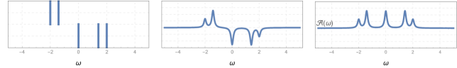
Figure 1: The spectral function of the Green’s function is a collection of infinite peaks, here pictorially depicted in the first panel. When the $\eta$ parameter is considered finite, one has a sum of Lorenztian functions in the upper (‘removal peaks’) and the lower half plane (‘addition peaks’), as in the second panel. The smoothed spectral function, for which also addition peaks lie on the upper half plane, is depicted in the last panel. The absolute scale of these spectral functions is irrelevant, as it depends on the unphysical $\eta$ parameter, and from here on values on the $y$-axis will always be omitted.

From that, we define the average absolute deviation $\sigma$ as follow:

$$\sigma:=\frac{\int d\omega\left|\mathpzc{A}_{exact}(\omega)-\mathpzc{A}_{approx}(\omega)\right|}{\int d\omega\left|\mathpzc{A}_{exact}(\omega)\right|}.$$ (27)

This will be used as parameter to quantify the goodness of an approximation: the higher is $\sigma$, the worst will be considered the corresponding approximation. In figure 2 we report a particularly neat example, the case with L=6, N=2, U/t=4 that illustrates the connection between the parameter $\sigma$ and the intuitive notion of ‘good approximate spectral function’, also providing a visual scale of reference for some representative values of $\sigma$.

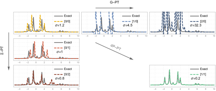
Figure 2: The function $\mathpzc{A}(\omega)$ is here plotted for different approximations in the case $L=6$, $N=2$, $U/t=4$.

The criterion is obviously somehow arbitrary, for certain details of the spectral function (position of the quasiparticle peaks, existence of satellites,…) may be of greater importance in certain situations; nonetheless it is general enough to provide an indication of the behaviour of the three approaches under study under generic circumstances.

Concerning the calculation of the approximate spectral functions, two remarks are in order. First, G-PT leads to approximate Green’s functions that cannot be written in terms of poles, while $\Sigma$-PT and dP-PT always lead to approximations that can be reduced to sum of poles, even though we do not always do it in practice, the effects being negligible. Second, in case of degeneracy, the expression (16) can be divergent, but we found that introducing a simple cutoff $\epsilon$ in formula (16) as $(\epsilon^{+}-\epsilon^{-})\to(\epsilon^{+}-\epsilon^{-}+\epsilon)$ and setting it to zero after the calculation of the Green’s function is sufficient to always get a finite result.

III.3 Choice of the basis

The Green’s function of the Hubbard model (23) has been here defined in the so called ‘site’ basis. Any Bogolioubov transformation of the ladder operators induces a new basis, which results in a rotation of the matrix $\{G_{ij}(\omega)\}$. The choice of the basis does not affect the spectral function, which is calculated from the trace of the Green’s function. However, Padé approximants built in different basis are inequivalent. This rises the question: is there a basis in which Padé approximants (not necessarily diagonal ones, but also G-PT and $\Sigma$-PT) work better? To attempt to reply to this question, we looked at the case of $L=2$, also known as Hubbard ‘dimer’.

For two sites the model is simple enough to admit an analytic solution and in Appendix LABEL:app:dimer we show the groundstates, labelled by the number of particles $\langle\hat{N}\rangle$ and, in case of degeneracy, the spin polarization $\langle\hat{S}_{z}\rangle$. Padé approximants can be calculated directly from the expression of $G$ one obtains simplifying (23) with those groundstates rather than using many-body perturbation theory (1). This allows to easily calculate approximants of very high order. Moreover, approximants in different basis can be calculated by considering rotations of $G$. A simple Bogolioubov transformation, reported in Appendix LABEL:app:dimer, is sufficient to make $G$ diagonal, independently of the number of particles and interaction strength. The fact that such a transformation does not depend on $U$ implies that also $G_{0}$ is diagonal in this basis.

Such a specific basis is particularly relevant because we found that, in the case of the dimer, while G-PT is not affected by a change of basis, both $\Sigma$-PT and dP-PT work better in this basis than any other. In fact, dP-PT converged to the exact result in only one step, namely $P_{[1/1]}[G_{0}]=G$, for $L=2$, $N=0,1,2,3,4$, as shown in Appendix LABEL:app:dimer for the representative case $N=2$. Such a remarkable property of this basis for the case $L=2$ suggested us to formulate the following conjecture: Padé approximants work best in the basis in which the noninteracting Green’s function is diagonal, irrespective of the number of sites or particles. From now on, we shall assume that and all calculations for $L>2$ will be shown only in the basis in which $G_{0}$ is diagonal.

III.4 Approximations comparison

Combining formulae (10,15,16,18) with $v^{m.f.}_{ij}=0$ we have an explicit expression for the functional $P_{[1/1]}$ that also applies to the Hubbard model. Such an approximant is made with the same amount of information (i.e. same diagrams) contained in the second order expansion of $\Sigma$ or $G$, denoted by $[0/2]$ and $[2/0]$ in the Padé notation. To compare the behaviour of the different expansions G-PT, $\Sigma$-PT and dP-PT we shall then consider the following sequences:

• $([0/0],[1/0],[2/0])$ for G-PT,

• $([0/0],[0/1],[0/2])$ for $\Sigma$-PT,

• and $([0/0],[1/1])$ for dP-PT.

We have calculated the deviation $\sigma$, as defined in (27), for the spectral functions arising from the corresponding approximations to the Green’s function, for all rings ($L=4,6,8,10$) and fillings ($N=2,4,...,2L-2$), in three different regimes of interaction: a weak, $U=0.1$, an intermediate, $U=1$, and a strong coupling, $U=10$, in units of $t$. For a given approximation $[N/M]$ and interaction strength $U$, the values of $\sigma$ for different sites and particles are here plotted on a single panel, arranged as reported in legend 3. This allows to get an idea of a specific approximation for a given interaction strength for all systems considered at a glance. Panels are then grouped for sequence of approximations, G-PT in fig. 4, $\Sigma$-PT in fig. 5 and dP-PT in fig. 6. Numerical values are explicitly reported in Appendix LABEL:app:data.

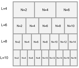
Figure 3:

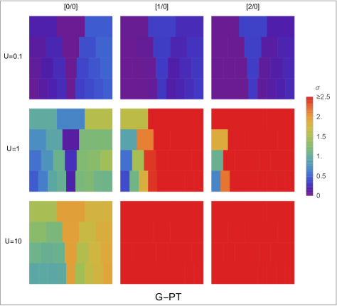
Figure 4:

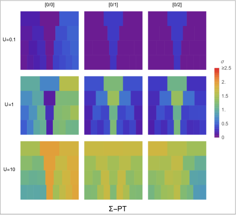
Figure 5:

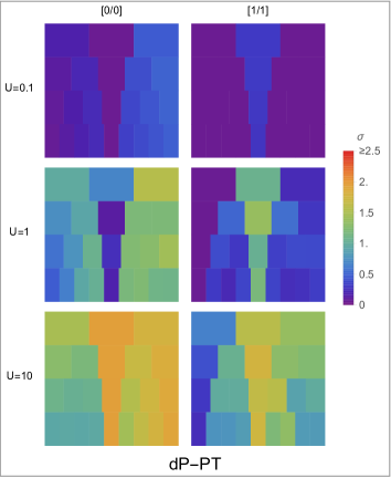
Figure 6:

Recalling that the closer to 0 (blue in plots) the better is the approximation, we recognize the following trends:

• all approximations deteriorate with increasing $U$;

• varying the number of sites $L$ does not seem to change the quality of the approximations; a higher number of sites only seems to increase the ‘definition’ of the plots;

• almost all approximations deteriorates when approaching the half-filling case;

• G-PT leads to meaningful results only in the weakly coupling regime, while $\Sigma$-PT and dP-PT lead to sensible approximations also in the intermediate and strong one;

• $\Sigma$-PT seems to have a slow convergence rate; namely the term $[0/2]$ does not improve over $[0/1]$ as much as $[0/1]$ does over $[0/0]$;

• dP-PT seems to have a higher rate of convergence (even when compared with the sequence $([0/0],[0/2])$), especially in the low filling cases ($N<L$);

• the higher the $U$ the better is dP-PT over $\Sigma$-PT.

A more direct comparison of $\Sigma$-PT and dP-PT is reported in figure 7, top panel.

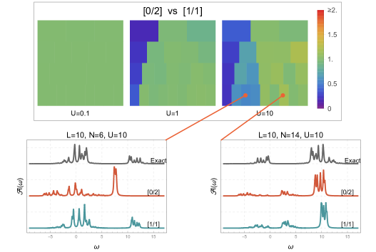
Figure 7: Top panel The ratio $\sigma_{[1/1]}/\sigma_{[0/2]}$ is plotted. For most cases this is less than one (green to blue color), indicating that $[1/1]$ provides a better estimate of the exact function than $[0/2]$. Bottom panel The spectral functions $\mathpzc{A}(\omega)$ in two cases representative of the situations $\sigma_{[1/1]}/\sigma_{[0/2]}<1$ and $\sigma_{[1/1]}/\sigma_{[0/2]}>1$ are plotted, for a better visual reference of the approximations.

As anticipated, $\Sigma$-PT is generally worst than dP-PT, especially for low fillings and high values of $U$. The cases in which $\Sigma$-PT is better are only a few and the improvement is not as much as that of dP-PT in other cases, as exemplified in the bottom panels of figure 7.

In absolute terms, $[1/1]$ leads to a decent approximation in most cases (as seen in figures 2 and 7), but, like all other approximations here considered, has serious problems in capturing the half-filling case, as one can see by comparing the first two top curves of figure 8. Even though the purpose of our study is to compare dP-PT to other perturbative approaches and not necessarily to provide precise estimates in absolute terms, we would like to focus a bit more on the half-filling case which in general (i.e. not just rings) bares special physical relevance scalettar. For instance, for $L=N=4$, the gap, defined as the energy difference between first addition and last removal peaks, is zero for $U=0$ but positive for $U>0$, which can be regarded as a sign of strong correlation. In such a case, shown in figure 8 for $U/t=4$, the approximant $P_{[1/1]}[G_{0}]$ does not capture the (anti)symmetry of the exact spectrum, nor the fact that addition and removal peaks are well separated by the gap, leading to a spectral function that one may deem as quite far from the exact one.

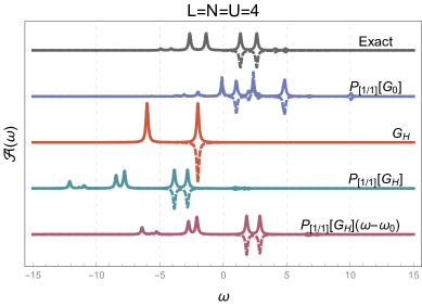
Figure 8: Various approximated spectral functions are compared to the exact one in the case $L=N=U/t=4$. To distinguish addition from removal peaks, the former are plotted in dashed lines in the lower half of the plane.

It is legitimate to expect that higher order dP-PT approximants correct these problems and converge towards the exact function, even though we have no elements to actually prove that and, even then, that convergence is practically achievable. On the other hand, for all half-filled systems here considered, we did notice that a sensible improvement comes already from considering a starting point for $P_{[1/1]}$ different from the pure noninteracting Green’s function. By taking $G_{H}$, defined as solution to the equation

$$G_{H}=G_{0}+G_{0}\Sigma_{H}[G_{H}]G_{H}$$ (29)

with

$$\Sigma^{(H)}_{ij}[g]:=-\sum_{kl}\int\!\!\!\!\!\!\!\leavevmode\hbox to10.84pt{\vbox to7.74pt{\text{[drawing]}}}\;\frac{d\omega^{\prime}}{2\pi}ig_{kl}(\omega^{\prime})v_{ilkj}$$ (30)

and building $P_{[1/1]}[G_{H}]$ using formulae (10,15,16,18) with $v^{m.f.}_{ij}=v^{\rm H}_{ij}=-i\delta_{ij}\Sigma^{(H)}_{ij}[g]$, one gets to a spectral function that partially restores the (anti)symmetry of the spectral function and correctly opens a gap between addition and removal peaks, as one can see in the penultimate (from top) curve of figure 8. Finally, an overall shift with no physical significance can be tuned to give rise to what we would deem as quite a decent approximation to the exact function. By comparing $P_{[1/1]}[G_{H}]$ to $P_{[0/0]}[G_{H}]$, which is simply $G_{H}$ (third curved in the plot), it seems then reasonable to expect that of $P_{[n/n]}[G_{H}]$ for $n>1$ would provide even better approximations to the exact $G$.

IV Conclusions

Padé approximants have proved to be an effective tool to get estimates of unknown functions in many fields of physics an mathematics bakergraves; baker1971. Their use in the calculation of electronic properties has been only partially explored, and in particular in the calculation of Green’s functions it has been limited so far as ancillary tool, like for the extrapolation of the analytic continuation of the Matsubara Green’s functions, or to model systems (see, for instance, goodson2012; schott2016; pavlyukh2017 and references therein.)

We have here presented a way to build Padé approximants of Green’s functions that generalizes the standard approximations based on the perturbative expansion of $G$ or the self-energy $\Sigma$ and provides a general framework suitable for model as well as for real systems. Moreover, we put forth the conjecture that, among all possible Padé approximants $[p/q]$ of given order $p+q$ of the Green’s function, diagonal ones, $p=q$, offer the best approximation. As preliminary test, we compared diagonal Padé approximants of order $[1/1]$ against approximations arising from direct perturbative expansion of $G$ and perturbative expansion of the self-energy of equivalent order for a series of solvable models, namely Hubbard rings with various number of sites, fillings and interaction strength, whose exact Green’s functions are (numerically) known. Based on a measure of likeness of spectral functions, we found indeed that in general the diagonal Padé approximant offered the most reliable approximation. In the great majority of cases it overcomes the other approximations, for all remaining cases still being quite close to the best (second-order $\Sigma$-PT). Particularly good results were obtained for high values of the interaction $U\gg t$ and low fillings $N<L$, irrespectively of the number $L$ of sites. We also presented a case of physical relevance ($L=N=U/t=4$) in which the approximant $[1/1]$ built on a mean field, rather than completely noninteracting, Green’s function greatly improves the otherwise not so good, in absolute terms, approximation.

Diagonal Padé approximants of the Green’s function were not directly built on some physical principle and in fact their physical interpretation as a resummation of certain terms of the pertubative series needs further investigation. On one hand this might make uncomfortable who would try to anticipate its behavior on a specific system. On the other hand one can say, in a rather optimistic attitude, that there is great potential in an approximation that is not designed around specific features of a class of systems. The performance of $[1/1]$ on the model studied in this work is a first prove of that.

A more tangible advantage of diagonal Padé approximants $[N/N]$ is that they are systematically improvable by increasing the order $N$. In this regard, we also argued that the computational cost increase implied by the rising of the order $N$ would probably remain moderate for a few orders. This is of capital importance in view of having a reliable, predictive tool.

In fact, the spreading of approximations based on the second-order expansion of the self-energy for a wide range of applications (from nuclear soma1 to molecular phillips2014 to periodic systems rusakov2016) suggests that already $P_{[1/1]}$, which in our study improves on $[0/2]$ almost in all cases, may already provide a competitive approximation, in all those situations and beyond.

In conclusions, we believe that diagonal Padé approximants certainly deserve more attention in the study of the many-body problem, as they may provide an effective new route for designing reliable, systematic approximations within the framework of standard perturbation theory.

Appendix A

When projected on a basis and Fourier-transformed to frequency space, diagrams (13) can be written as:

$$\Sigma^{(1)}_{ij}\equiv\includegraphics[scale={0.5}]{diaga}+\includegraphics[scale={0.5}]{diagb}+\includegraphics[scale={0.8}]{diagc}=\sum_{kl}\int\!\!\!\!\!\!\!\leavevmode\hbox to10.84pt{\vbox to5.72pt{\text{[drawing]}}}\;\frac{d\omega^{\prime}}{2\pi}ig_{kl}(\omega^{\prime})\left(v_{iljk}-v_{ilkj}\right)-i\delta_{ij}v^{m.f.}_{ij}$$ (31)

and

$$\Sigma^{(2)}_{ij}(\omega)\equiv\Sigma^{(2.1)}_{ij}+\Sigma^{(2.2)}_{ij}+\Sigma^{(2.3)}_{ij}+\Sigma^{(2.4)}_{ij}(\omega)+\Sigma^{(2.5)}_{ij}+\Sigma^{(2.6)}_{ij}(\omega)+\Sigma^{(2.7)}_{ij}+\Sigma^{(2.8)}_{ij}$$ (32)

rClΣ^(2.1)_ij&≡ = -∑_nopqrs∫​​​​​​​  dω’dω”4π2 g_no(ω’)g_pq(ω”)g_rs(ω’)v_iorjv_qsnp rClΣ^(2.2)_ij&≡ = ∑_nopqrs∫​​​​​​​  dω’dω”4π2g_no(ω’)g_pq(ω”)g_rs(ω’)v_iojrv_qsnp rClΣ^(2.3)_ij&≡ = ∑_nopqrs∫​​​​​​​  dω’dω”4π2 g_no(ω’)g_pq(ω”)g_rs(ω”)v_iqrjv_osnp rClΣ^(2.4)_ij(ω)&≡ = -∑_nopqrs∫​​​​​​​  dω’dω”4π2g_no(ω+ω’-ω”)g_pq(ω”)g_rs(ω’)v_isnpv_oqrj rClΣ^(2.5)_ij&≡ = -∑