Benchmark study of an auxiliary-field quantum Monte Carlo technique for the Hubbard model with shifted-discrete Hubbard-Stratonovich transformations

Abstract

Within the ground-state auxiliary-field quantum Monte Carlo technique, we introduce discrete Hubbard-Stratonovich transformations (HSTs) that are suitable also for spatially inhomogeneous trial functions. The discrete auxiliary fields introduced here are coupled to local spin or charge operators fluctuating around their Hartree-Fock values. The formalism can be considered as a generalization of the discrete HSTs by Hirsch  [J. E. Hirsch, Phys. Rev. B 28, 4059 (1983)] or a compactification of the shifted-contour auxiliary-field Monte Carlo formalism by Rom et al.  [N. Rom et al., Chem. Phys. Lett. 270, 382 (1997)]. An improvement of the acceptance ratio is found for a real auxiliary field, while an improvement of the average sign is found for a pure-imaginary auxiliary field. Efficiencies of the different HSTs are tested in the single-band Hubbard model at and away from half filling by studying the staggered magnetization and energy expectation values, respectively.

I Introduction

The numerical solution of the Hubbard model with strong correlations is one of the most challenging issues in the theory of strongly correlated electron systems LeBlanc et al. (2015); Zheng et al. (2017). Attempts to determine the ground state are often based on iterative techniques based on a repeated application of a short imaginary time propagator, or by using the simple power method and more advanced Krylov-subspace techniques, as, for instance the Lanczos algorithm, where a Hamiltonian operator is repeatedly applied to a properly chosen trial state. In both cases the ground-state component of the trial state is filtered out after several iterations.

Among these projection techniques, the auxiliary-field quantum Monte Carlo (AFQMC) Sugiyama and Koonin (1986); Sorella et al. (1989); Imada and Hatsugai (1989); Becca and Sorella (2017) is one of the most powerful schemes, as it allows us to study, for example, the ground-state properties of the Hubbard model with several thousands electrons and lattice sites, when the negative-sign problem is absent Sorella et al. (2012); Otsuka et al. (2016, 2018). In the ground-state AFQMC, even if the Hamiltonian is the same, there exists some arbitrariness in choosing the trial wave function and the type of auxiliary fields (e.g., real, complex, continuous, or discrete). Experience has shown that an appropriate choice of these ingredients may significantly improve the efficiency of the Monte Carlo simulations Shi and Zhang (2013).

It has been demonstrated Qin et al. (2016a); Zheng et al. (2017) that a Slater-determinant obtained from an unrestricted Hartree-Fock (UHF) approximation Xu et al. (2011) provides a good trial wave function for the doped Hubbard model in the constrained-path AFQMC Zhang et al. (1997). Recently, for a particular parameter set at doping $\delta=1/8$ and electron-electron repulsion $U/t=8$, the ground state of the Hubbard model on the square lattice has been predicted to exhibit a vertical stripe order Zheng et al. (2017), where the stripe states with periods $\lambda=5,6,7$ and $8$ in units of the lattice constant are nearly degenerate, while a spatially homogeneous $d$-wave superconducting state should have, according to their study, a higher energy. Recent variational Monte Carlo (VMC) calculations Zhao et al. (2017); Ido et al. (2018); Darmawan et al. (2018) have also shown that various vertical-stripe orders with different periods appear depending on the doping and the hopping parameter. In most of the calculations in Ref. Zheng et al. (2017), the symmetry of finite-size clusters is broken due to the use of UHF trial wave functions or by applying pinning magnetic fields, and the results are extrapolated to the thermodynamic limit. The success of utilizing symmetry-broken wave functions is rather surprising, because symmetry breakings do not occur in the exact ground state of finite-size systems. The similar issue is known as the symmetry dilemma in first-principles calculations for molecules Perdew et al. (1995); Carrascal et al. (2015). Recently, it has been shown that the quality of the trial wave function can be improved by restoring the symmetries that are once broken by UHF or mean-field treatments Tahara and Imada (2008); Rodríguez-Guzmán et al. (2012); Shi et al. (2014). However, in the present work, we do not enter into the issue on symmetry breakings of trial wave functions, and rather focus on the arbitrariness of the auxiliary field to improve the efficiency of AFQMC simulations with such symmetry-broken trial wave functions.

The way of transforming a quartic interaction term into a quadratic one via the Hubbard-Stratonovich transformation (HST) Hubbard (1959) is not unique and affects the efficiency of simulations Hirsch (1983); Motome and Imada (1997); Held and Vollhardt (1998); Sakai et al. (2004); Han (2004); Broecker and Trebst (2016). Recently the popularity of this technique is substantially increased, because it has been realized that, with continuous auxiliary fields, one can treat interaction terms beyond the on-site Hubbard interaction, up to the complete treatment of the long-range Coulomb interaction Buividovich and Polikarpov (2012); Ulybyshev et al. (2013); Hohenadler et al. (2014); Tang et al. (2015, 2018), or of the long-range electron-phonon interaction Batrouni and Scalettar (2019), and even both of them on the same footing Karakuzu et al. (2018a), without being vexed by the sign problem in a certain parameter region on bipartitle lattices. Interestingly, such a parameter region coincides with the one where rigorous statements on the ground state of an extended Hubbard-Holstein model are available Lieb (1989); Miyao (2018). It is also noteworthy that, even when the sign problem cannot be eliminated completely, continuous auxiliary fields with a proper shift Rom et al. (1997, 1998); Baer et al. (1998) can improve the efficiency of simulations compared to the one without the shift. A similar idea has been employed also in the AFQMC Zhang and Krakauer (2003); Motta et al. (2014) within the constrained-path approximation Zhang et al. (1997).

In this paper, we introduce shifted-discrete HSTs, where auxiliary fields are coupled to the fluctuation of local spin or charge. The method is applied for AFQMC simulations of the Hubbard model on the square lattice. It is shown that the shifted-discrete HSTs can improve the efficiency of the AFQMC simulations. Moreover we present results on the magnetic order parameter as a function of $U/t$ with high statistical accuracy, that represents important benchmark, useful also for comparison with experiments.

The rest of the paper is organized as follows. In Sec. II, the Hubbard model is defined and the AFQMC method is described. In Sec. III, the shifted-discrete HSTs are introduced. In Sec. IV, numerical results of the AFQMC simulations for the Hubbard model are presented. Section V is devoted to conclusions and discussions.

II Model and method

We consider the Hubbard model whose Hamiltonian is defined by $\hat{H}=\hat{K}+\hat{V}$, where

$$\hat{K} = -t\sum_{\langle ij\rangle,\sigma}\left(\hat{c}_{i\sigma}^{\dagger}\hat{c}_{j\sigma}+{\rm H.c.}\right),$$ (1)

$$\hat{V} = U\sum_{i}\hat{n}_{i\uparrow}\hat{n}_{i\downarrow},$$ (2)

$\hat{c}_{i\sigma}^{\dagger}$ ($\hat{c}_{i\sigma}$) creates (annihilates) a fermion with site index $i$ and spin index $\sigma(=\uparrow,\downarrow)$, $\hat{n}_{i\sigma}=\hat{c}_{i\sigma}^{\dagger}\hat{c}_{i\sigma}$, $t$ is the hopping parameter between the nearest-neighbor sites on the square lattice and $U>0$ is the on-site electron-electron repulsion. We consider the Hubbard model on $N=L\times L$-site clusters. Boundary conditions will be specified for each calculation in Sec. IV. The lattice constant is set to be unity.

In the AFQMC, the expectation value of an operator $\hat{O}$ is calculated as

$$\langle\hat{O}\rangle_{\beta}=\frac{\langle\Psi_{\rm T}|\mathrm{e}^{-\frac{\beta}{2}\hat{H}}\hat{O}\mathrm{e}^{-\frac{\beta}{2}\hat{H}}|\Psi_{\rm T}\rangle}{\langle\Psi_{\rm T}|\mathrm{e}^{-\beta\hat{H}}|\Psi_{\rm T}\rangle},$$ (3)

where $\beta$ is the projection time and $|\Psi_{\rm T}\rangle$ is a trial wave function. If $\beta$ is infinitely large, one can obtain the ground-state expectation value as long as $|\Psi_{\rm T}\rangle$ has a finite overlap with the ground state Horn and Weinstein (1984). If $\beta$ is finite, the results depend on the trial wave function (see for example Ref. Weinberg and Sandvik (2017)). If $\beta=0$, Eq. (3) reduces to the expectation value of $\hat{O}$ with respect to the trial wave function.

At finite dopings, $|\Psi_{\rm T}\rangle$ is obtained by solving the eigenvalue problem of the following UHF Hamiltonian self consistently:

$$\hat{H}_{\rm UHF}=\hat{K}+U_{\rm eff}\sum_{i}\left(\langle\hat{n}_{i\uparrow}\rangle_{0}\hat{n}_{i\downarrow}+\hat{n}_{i\uparrow}\langle\hat{n}_{i\downarrow}\rangle_{0}-\langle\hat{n}_{i\uparrow}\rangle_{0}\langle\hat{n}_{i\downarrow}\rangle_{0}\right),$$ (4)

where $U_{\rm eff}$ is an arbitrary parameter and the expectation value $\langle\cdots\rangle_{0}$ in Eq. (4) is defined in Eq. (3) with $\beta=0$. A fine tuning of $U_{\rm eff}$ can improve the quality of the trial wave function Qin et al. (2016a). We set $U_{\rm eff}/t=2.5$ which has turned out to provide a good trial wave function for the doped cases studied here, in the sense that the energy expectation value decreases quickly with increasing $\beta$. By adding a small bias in the initial condition for the self consistent UHF loop to pin the direction of the stripe, $|\Psi_{\rm T}\rangle$ shows a vertical stripe order with period $\lambda=8$ around $\delta=1/8$ doping on the $16\times 16$ cluster.

At half filling, $|\Psi_{\rm T}\rangle$ is obtained as a ground state of non-interacting electrons on the square lattice under a staggered magnetic field along the spin-quantized axis ($z$ direction):

$$\hat{H}_{\rm MF}=\hat{K}-\Delta_{\rm AF}\sum_{i}(-1)^{i}(\hat{n}_{i\uparrow}-\hat{n}_{i\downarrow}),$$ (5)

where $(-1)^{i}=1(-1)$ if the site $i$ belongs to the $A$ ($B$) sublattice and $\Delta_{\rm AF}$ can be chosen arbitrarily. The value of $\Delta_{\rm AF}$ will be specified with the numerical results in Sec. IV.

By using the second-order Suzuki-Trotter decomposition Trotter (1959); Suzuki (1976), the imaginary-time propagator can be expressed as

$$\mathrm{e}^{-\beta\hat{H}}=\prod_{n=1}^{N_{\tau}}\left(\mathrm{e}^{-\frac{\Delta_{\tau}}{2}\hat{K}}\mathrm{e}^{-\Delta_{\tau}\hat{V}}\mathrm{e}^{-\frac{\Delta_{\tau}}{2}\hat{K}}\right)+O\left(\Delta_{\tau}^{2}\right),$$ (6)

where the projection time $\beta$ is discretized into $N_{\tau}$ time slices and $\Delta_{\tau}=\beta/N_{\tau}$. For the doped cases, we set $\Delta_{\tau}t=0.05$ so that the discretization error is within statistical errors. For the half filled case, we perform extrapolations of $\Delta_{\tau}\to 0$ to eliminate the discretization error, which becomes non negligible for large $U/t$ as compared to statistical or extrapolation errors for the results shown in Sec. IV.2. An HST is applied to $\mathrm{e}^{-\Delta_{\tau}\hat{V}}$ and the summation over the auxiliary fields is performed by the Monte Carlo method with the importance sampling, where a proposed auxiliary-field configuration is accepted or rejected according to the Metropolis algorithm. In the next Section, we introduce shifted-discrete HSTs for $\mathrm{e}^{-\Delta_{\tau}\hat{V}}$.

III Shifted-discrete Hubbard-Stratonovich transformations

In this Section we derive shifted-discrete HSTs which couple the auxiliary field to the local spin fluctuation in Sec. III.1 and to the local charge fluctuation in Sec. III.2. Although the two HSTs can be formulated almost in parallel, we provide both of them separately for completeness.

III.1 Auxiliary field coupled to spin fluctuation

The Hubbard interaction in Eq. (2) can be written as

$$\hat{V}= - \frac{U}{2}\sum_{i}\left[\left(\hat{n}_{i\uparrow}-\hat{n}_{i\downarrow}-\tilde{m}_{i}\right)^{2}-\tilde{m}_{i}^{2}\right]$$ (7)

$$+ \frac{U}{2}\sum_{i}\left[(1-2\tilde{m}_{i})\hat{n}_{i\uparrow}+(1+2\tilde{m}_{i})\hat{n}_{i\downarrow}\right]$$

where $\tilde{m}_{i}$ is an arbitrary number. Then $\mathrm{e}^{-\Delta_{\tau}V}$ can be written as

$$\mathrm{e}^{-\Delta_{\tau}\hat{V}} = \mathrm{e}^{\frac{\Delta_{\tau}U}{2}\sum_{i}\left[(\hat{n}_{i\uparrow}-\hat{n}_{i\downarrow}-\tilde{m}_{i})^{2}-\tilde{m}_{i}^{2}\right]}$$ (8)

$$\times \mathrm{e}^{-\frac{\Delta_{\tau}U}{2}\sum_{i}(1-2\tilde{m}_{i})\hat{n}_{i\uparrow}}\mathrm{e}^{-\frac{\Delta_{\tau}U}{2}\sum_{i}(1+2\tilde{m}_{i})\hat{n}_{i\downarrow}}.$$

Let us consider the first exponential factor in the right-hand side of Eq. (8). For each site $i$, we consider the following HST:

$$C_{i}\mathrm{e}^{-\frac{\Delta_{\tau}U}{2}\tilde{m}_{i}^{2}}\mathrm{e}^{\frac{\Delta_{\tau}U}{2}(\hat{n}_{i\uparrow}-\hat{n}_{i\downarrow}-\tilde{m}_{i})^{2}}=\frac{1}{2}\sum_{s_{i}=\pm 1}\mathrm{e}^{\alpha_{i}s_{i}(\hat{n}_{i\uparrow}-\hat{n}_{i\downarrow}-m_{i})},$$ (9)

where $s_{i}=\pm 1$ is the discrete auxiliary field, and the undetermined four parameters $\alpha_{i}$, $m_{i}$, $\tilde{m}_{i}$ and $C_{i}$ are related through the following three equations (see Appendix A for derivation):

$$\frac{\cosh{\alpha_{i}(1-m_{i})}\cosh{\alpha_{i}(1+m_{i})}}{\cosh^{2}{\alpha_{i}m_{i}}}=\mathrm{e}^{\Delta_{\tau}U},$$ (10)

$$\tilde{m_{i}}=\frac{1}{2\Delta_{\tau}U}\ln\frac{\cosh{\alpha_{i}(1+m_{i})}}{\cosh{\alpha_{i}(1-m_{i})}},$$ (11)

$$C_{i}=\mathrm{e}^{\Delta_{\tau}U\tilde{m}^{2}/2}\cosh{\alpha_{i}m_{i}}.$$ (12)

Therefore, if say $m_{i}$ is given, $\alpha_{i}$, $\tilde{m}_{i}$, and $C_{i}$ are determined from Eqs. (10)-(12). Finally we obtain

$$\mathrm{e}^{-\Delta_{\tau}\hat{V}}\propto\prod_{i}\sum_{s_{i}=\pm 1}\mathrm{e}^{\left[\alpha_{i}s_{i}-\frac{\Delta_{\tau}U}{2}(1-2\tilde{m}_{i})\right]\hat{n}_{i\uparrow}+\left[-\alpha_{i}s_{i}-\frac{\Delta_{\tau}U}{2}(1+2\tilde{m}_{i})\right]\hat{n}_{i\downarrow}-\alpha s_{i}m_{i}},$$ (13)

Note that in general $m_{i}\not=\tilde{m}_{i}$ and $C_{i}$’s are irrelevant for results of simulations because they cancel out from the numerator and the denominator in Eq. (3). If $m_{i}=0$, the HST reduces to the one introduced by Hirsch Hirsch (1983). However, the arbitrariness of $m_{i}$ can be utilized to improve the efficiency of AFQMC simulations as shown in Sec. IV.

In the right-hand side of Eq. (13), the auxiliary field $\alpha_{i}s_{i}$ is shifted by $\Delta_{\tau}U\tilde{m}_{i}$ as compared to the case of $m_{i}=\tilde{m}_{i}=0$. To obtain more physical intuitions for $m_{i}$, we rewrite the exponent of the right-hand side of Eq. (13) as

$$\alpha_{i}s_{i}\left(\hat{n}_{i\uparrow}-\hat{n}_{i\downarrow}-m_{i}\right)+\Delta_{\tau}U\tilde{m}_{i}\left(\hat{n}_{i\uparrow}-\hat{n}_{i\downarrow}\right)-\frac{\Delta_{\tau}U}{2}\left(\hat{n}_{i\uparrow}+\hat{n}_{i\downarrow}\right).$$ (14)

In the first term, the auxiliary field $\alpha_{i}s_{i}$ is coupled to the fluctuation of the local magnetization $(\hat{n}_{i\uparrow}-\hat{n}_{i\downarrow}-m_{i})$, while the shift of the local magnetization by $-m_{i}$ in the first term is compensated by the spatially inhomogeneous magnetic field $\Delta_{\tau}U\tilde{m}_{i}$ in the second term.

We set the parameter $m_{i}$ as the local magnetization in the trial wave function

$$m_{i}=\langle\hat{n}_{i\uparrow}-\hat{n}_{i\downarrow}\rangle_{0}.$$ (15)

This $m_{i}$ can be easily calculated and is expected to stabilize the simulation by keeping the first term in Eq. (14) “small” during the imaginary-time evolution. For a given $m_{i}$, $\alpha_{i}$ can be determined from Eq (10), $\tilde{m}_{i}$ from Eq. (11), and $C_{i}$ from Eq. (12). The solution $\alpha_{i}$ of Eq. (10) can be found by the Newton method with an initial guess $\alpha_{i,{\rm initial}}=\cosh^{-1}\mathrm{e}^{\Delta_{\tau}U/2}$, for example.

III.2 Auxiliary field coupled to charge fluctuation

In this subsection, $\alpha_{i}$ and $C_{i}$ will be re-defined. The Hubbard interaction in Eq. (2) can be written as

$$\hat{V} = \frac{U}{2}\sum_{i}\left[\left(\hat{n}_{i\uparrow}+\hat{n}_{i\downarrow}-\tilde{n}_{i}\right)^{2}-\tilde{n}_{i}^{2}\right]$$ (16)

$$- \frac{U}{2}\sum_{i}\left[(1-2\tilde{n}_{i})\hat{n}_{i\uparrow}+(1-2\tilde{n}_{i})\hat{n}_{i\downarrow}\right]$$

where $\tilde{n}_{i}$ is an arbitrary number. Then $\mathrm{e}^{-\Delta_{\tau}V}$ can be written as

$$\mathrm{e}^{-\Delta_{\tau}\hat{V}} = \mathrm{e}^{-\frac{\Delta_{\tau}U}{2}\sum_{i}\left[(\hat{n}_{i\uparrow}+\hat{n}_{i\downarrow}-\tilde{n}_{i})^{2}-\tilde{n}_{i}^{2}\right]}$$ (17)

$$\times \mathrm{e}^{\frac{\Delta_{\tau}U}{2}\sum_{i}(1-2\tilde{n}_{i})\hat{n}_{i\uparrow}}\mathrm{e}^{\frac{\Delta_{\tau}U}{2}\sum_{i}(1-2\tilde{n}_{i})\hat{n}_{i\downarrow}}.$$

Let us consider the first exponential factor in the right-hand side of Eq. (17). For each site $i$, we consider the following HST:

$$C_{i}\mathrm{e}^{\frac{\Delta_{\tau}U}{2}\tilde{n}_{i}^{2}}\mathrm{e}^{-\frac{\Delta_{\tau}U}{2}(\hat{n}_{i\uparrow}+\hat{n}_{i\downarrow}-\tilde{n}_{i})^{2}}=\frac{1}{2}\sum_{s=\pm 1}\mathrm{e}^{i\alpha_{i}s_{i}(\hat{n}_{i\uparrow}+\hat{n}_{i\downarrow}-n_{i})},$$ (18)

where $s_{i}=\pm 1$ is the discrete auxiliary field, and the undetermined four parameters $\alpha_{i}$, $n_{i}$, $\tilde{n}_{i}$ and $C_{i}$ are related through the following three equations (see Appendix A for derivation):

$$\frac{\cos{\alpha_{i}(2-n_{i})}\cos{\alpha_{i}n_{i}}}{\cos^{2}{\alpha_{i}(1-n_{i})}}=\mathrm{e}^{-\Delta_{\tau}U},$$ (19)

$$\tilde{n}_{i}=1-\frac{1}{2\Delta_{\tau}U}\ln\frac{\cos{\alpha_{i}n_{i}}}{\cos{\alpha_{i}(2-n_{i})}},$$ (20)

$$C_{i}=\mathrm{e}^{-\Delta_{\tau}U\tilde{n}_{i}^{2}/2}\cos{\alpha_{i}n_{i}}.$$ (21)

Therefore, if say $n_{i}$ is given, $\alpha_{i}$, $\tilde{n}_{i}$, and $C_{i}$ are determined from Eqs. (19)-(21). Finally we obtain

$$\mathrm{e}^{-\Delta_{\tau}\hat{V}}\propto\prod_{i}\sum_{s_{i}=\pm 1}\mathrm{e}^{\left[i\alpha_{i}s_{i}+\frac{\Delta_{\tau}U}{2}(1-2\tilde{n}_{i})\right]\hat{n}_{i\uparrow}+\left[i\alpha_{i}s_{i}+\frac{\Delta_{\tau}U}{2}(1-2\tilde{n}_{i})\right]\hat{n}_{i\downarrow}-i\alpha s_{i}n_{i}},$$ (22)

Note that in general $n_{i}\not=\tilde{n}_{i}$ and $C_{i}$’s are irrelevant for results of simulations because they cancel out between the numerator and the denominator in Eq. (3). If $n_{i}=1$, the HST reduces to the one introduced by Hirsch Hirsch (1983). However, the arbitrariness of $n_{i}$ can be utilized to improve the efficiency of AFQMC simulations as shown in Sec. IV.

In the right-hand side of Eq. (22), the auxiliary field $i\alpha_{i}s_{i}$ is shifted by $\Delta_{\tau}U(1-\tilde{n}_{i})$ as compared to the case of $n_{i}=\tilde{n}_{i}=1$. To obtain more physical intuitions for $n_{i}$, we rewrite the exponent of the right-hand side of Eq. (22) as

$$i\alpha_{i}s_{i}\left(\hat{n}_{i\uparrow}+\hat{n}_{i\downarrow}-n_{i}\right)+\Delta_{\tau}U(1-\tilde{n}_{i})\left(\hat{n}_{i\uparrow}+\hat{n}_{i\downarrow}\right)-\frac{\Delta_{\tau}U}{2}\left(\hat{n}_{i\uparrow}+\hat{n}_{i\downarrow}\right).$$ (23)

In the first term, the auxiliary field $i\alpha_{i}s_{i}$ is coupled to the fluctuation of the local density $(\hat{n}_{i\uparrow}+\hat{n}_{i\downarrow}-n_{i})$, while the shift of the local density by $-(1-n_{i})$ in the first term is compensated by the spatially inhomogeneous chemical potential $\Delta_{\tau}U(1-\tilde{n}_{i})$ in the second term.

We set the parameter $n_{i}$ as the local charge density in the trial wave function

$$n_{i}=\langle\hat{n}_{i\uparrow}+\hat{n}_{i\downarrow}\rangle_{0}.$$ (24)

This $n_{i}$ can be easily calculated and is expected to stabilize the simulation by keeping the first term in Eq. (23) “small” during the imaginary-time evolution. For a given $n_{i}$, $\alpha_{i}$ can be determined from Eq (19), $\tilde{n}_{i}$ from Eq. (20), and $C_{i}$ from Eq. (21). The solution $\alpha_{i}$ of Eq. (19) can be found by the Newton method with an initial guess $\alpha_{i,{\rm initial}}=\cos^{-1}\mathrm{e}^{-\Delta_{\tau}U/2}$, for example.

IV Numerical results

IV.1 Finite dopings

At finite dopings, the sign problem occurs Hirsch (1985); Loh et al. (1990). In the presence of the sign problem, the projection time $\beta$ cannot be taken as large as that for the half filled case because the average sign (of the statistical weight) decreases exponentially in $\beta$ Loh et al. (1990), otherwise the number of statistical samplings has be increased exponentially to keep the statistical error small. We set the maximum $\beta$ at which the average sign is $\sim 0.05$. It will be shown that even in the presence of the sign problem, the AFQMC can still provide a good upper bound of the ground-state energy.

Figure 1 shows the energy per site $E(\beta)=\langle\hat{H}\rangle_{\beta}/N$, the average sign, and the acceptance rate as a function of $\beta$ at $U/t=8$ for the $16\times 16$ cluster with $224$ electrons, corresponding to $\delta=1/8=0.125$. Note that since

$$\frac{\mathrm{d}E(\beta)}{\mathrm{d}\beta}=-\frac{1}{N}\left(\langle\hat{H}^{2}\rangle_{\beta}-\langle\hat{H}\rangle^{2}_{\beta}\right)\leqslant 0,$$ (25)

$E(\beta)$ is a decreasing function of $\beta$ and its slope $\mathrm{d}E(\beta)/\mathrm{d}\beta$ is proportional to the energy variance Horn and Weinstein (1984). The energies calculated by different HSTs coincide within the statistical errors, though their reachable $\beta$ is different, as shown in Fig. 1(a). In Fig. 1(b), the acceptance rate of the real auxiliary field with the shift (HST spin with shift) is increased the one from without the shift (HST spin without shift). The reason can be attributed to that since the first term of Eq. (14) with a relevant $m_{i}$ is expected to be “smaller” than that with $m_{i}=0$, the factor $\mathrm{e}^{\pm 2\alpha_{i}(\hat{n}_{i\uparrow}-\hat{n}_{i\downarrow}-m_{i})}$ is closer to unity, so that the fluctuation of the norm of the determinant ratio is stabilized. On the other hand, the shift of the real auxiliary field does not affect the average sign significantly because the shift does not affect the sign of the determinant ratio, as can be seen in Fig. 1(c). The situation is different for the pure-imaginary auxiliary fields. Without the shift (HST charge without shift), the average sign diminishes significantly, even at $\beta t=0.1$. By introducing the shift (HST charge with shift), the average sign is improved significantly. The reason can be attributed to that since the first term of Eq. (23) with a relevant $n_{i}$ is expected to be “smaller” than that with $n_{i}=1$, the factor $\mathrm{e}^{\pm 2i\alpha_{i}(\hat{n}_{i\uparrow}+\hat{n}_{i\downarrow}-n_{i})}$ is closer to unity, so that the fluctuation of the phase of the determinant ratio is stabilized. However, the average sign is still quite smaller than that with the real auxiliary fields. Although the acceptance rate is higher than the real auxiliary fields, the pure-imaginary fields may not be practical in the presence of the sign problem.

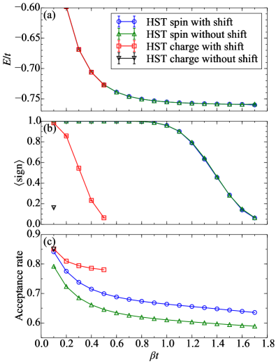
Figure 1: (a) The energy per site, (b) the average sign, and (c) the acceptance rate as a function of the projection time $\beta$ with different HSTs. Calculations are done on the $16\times 16$ cluster with $224$ electrons ($\delta=0.125$) at $U/t=8$.

To show the usefulness of the AFQMC with a short imaginary-time propagation, we make a comparison with the state-of-the-art variational wave functions for the Hubbard model Zhao et al. (2017); Ido et al. (2018). To this end, we move to the smaller doping with the larger $U/t$, where the more severe sign problem is expected. Figure 2 shows the energy per and the average sign as a function of $\beta$ at $U/t=10$ for the $16\times 16$ cluster with $228$ electrons, corresponding to $\delta=0.109375$. Here, only the shifted real auxiliary field is employed because it turned out to be the most efficient, as shown in Fig. 1 for $U/t=8$ and $\delta=0.125$. We use periodic- (antiperiodic-) boundary condition in the $x$ ($y$) direction to compare directly with the reference VMC results Zhao et al. (2017); Ido et al. (2018). Notice that our AFQMC energy, computed at finite projection time $\beta$ when the average sign is sufficiently large, respects the Ritz’s variational principle [see Eq. (3)], because it corresponds to the variational expectation value of $\hat{H}$ over the state $\mathrm{e}^{-\frac{\beta}{2}\hat{H}}|\Psi_{\rm T}\rangle/\langle\Psi_{\rm T}|\mathrm{e}^{-\beta\hat{H}}|\Psi_{\rm T}\rangle^{\frac{1}{2}}$. This is a useful property of an approximate technique that is not always satisfied, as for instance for the constrained-path AFQMC Zhang et al. (1997); Zhang and Krakauer (2003). At $\beta t=0.7$, where the average sign remains $\sim 0.99$, the AFQMC energy is already lower than the VMC energy without variance extrapolation. At $\beta t=1.1$, the AFQMC energy almost coincides with the VMC variance-extrapolated one, while the slope $\mathrm{d}E(\beta)/\mathrm{d}\beta$ is still finite, indicating that the AFQMC energy variance is nonzero [see Eq. (25)]. At $\beta t=1.5$, the AFQMC energy is $E/t=-0.6552(4)$, which is lower than the variance-extrapolated VMC energy $E/t=0.6538(9)$ Zhao et al. (2017) which may be compatible with our number within two standard deviations. This result suggest that the ground-state AFQMC method remains very useful for providing upper bound values of the ground-state energy even in the presence of the negative-sign problem.

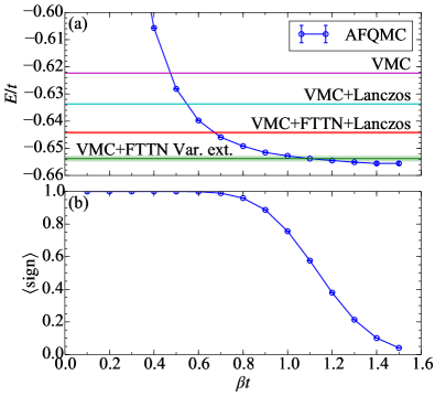
Figure 2: (a) The energy per site and (b) the average sign as a function of the projection time $\beta$. Calculations refer to the $16\times 16$ cluster with $228$ electrons ($\delta=0.109375$) at $U/t=10$. In (a), the horizontal lines and the shaded regions are the VMC energies and their error bars taken from Refs. Zhao et al. (2017); Ido et al. (2018). FTTN stands for fat-tree tensor network and Var. ext. for variance extrapolation.

IV.2 Half filling

At half filling, the sign problem is absent. Therefore the AFQMC can provide exact results which often serve as a reference benchmark for other numerical techniques. An excellent agreement in the ground-state energies of the two-dimensional Hubbard model between the AFQMC and other many-body techniques has been reported in Ref. LeBlanc et al. (2015). Moreover, within the AFQMC, the staggered magnetization $m$, i.e., the order parameter at half filling, can be estimated accurately by using the twist-averaged boundary condition for small $U/t$, e.g., $U\lesssim 4$ Qin et al. (2016b); Karakuzu et al. (2018b). However, for large $U/t$, AFQMC simulations still face a difficulty of large fluctuations of the magnetization, which often lead to a relatively large error bar in $m$ Qin et al. (2016b); LeBlanc et al. (2015). The same difficulty arises also in finite-temperature determinant QMC simulations Hirsch and Tang (1989); Varney et al. (2009). In previous works, in order to overcome the difficulty, a pinning-field method has been proposed with a clear improvement for the determination of $m$ in the thermodynamic limit Assaad and Herbut (2013); Wang et al. (2014). In the following, we report an accurate estimate $m$ especially for large $U/t$ by making use of a symmetry-broken trial wave function.

Figure 3 shows the staggered magnetization along the $z$ direction

$$m(\beta)=\frac{1}{2N}\sum_{i}(-1)^{i}\langle\hat{n}_{i\uparrow}-\hat{n}_{i\downarrow}\rangle_{\beta}$$ (26)

as a function of the Monte Carlo sweep with different HSTs. The calculations are done for $U/t=8$, $\beta t=24$, and $\Delta_{\tau}t=0.1$ on the $L=16$ cluster with periodic-boundary conditions. We use $\Delta_{\rm AF}/t=0.001$ to give a finite staggered magnetization in the trial wave function. This small value of $\Delta_{\rm AF}$ is effective to pin a sizable value of the finite size order parameter $m(0)$ because the single-particle states at $U/t=0$ have a large degeneracy ($\propto L$) at the Fermi level,and are therefore strongly renormalized upon an arbitrary small $\Delta_{\rm AF}$.

Since $m(0)$ is finite [see Eq. (5)], $m(\beta)$ remains finite even for finite $L$. Note that, at half filling, the HST in the charge channel with shift is equivalent to the one without shift because $n_{i}=1$. A very large equilibration time of $\sim 5000$ Monte Carlo sweeps is found for $m$ with the standard real HST coupled to the on-site electron spins. In this case, our shifted HST improves the equilibration time, allowing also higher acceptance rate (not shown) as in the doped cases, but the improvement is not really important. Amazingly, $m$ is equilibrated almost immediately for the complex HST coupled to the on-site electron charges. This result implies that this pure-imaginary auxiliary field, which was first introduced by Hirsch Hirsch (1983), is very useful to estimate $m$ at half filling for large $U/t$. Here we emphasize also that, not only the correlation time is highly reduced with this technique, but also fluctuations, thanks to this pinning strategy in the trial wave function, do not show any problem of large fluctuations, even at very large $U/t$ and values.

Figure 3: The staggered magnetization $m$ as a function of the Monte-Carlo sweep for the half-filled Hubbard model on the square lattice at $U/t=8$ with different HSTs. Calculations are done on the $16\times 16$ cluster with $\beta t=24$.

Figure 4 shows the finite-size scaling of $m$ for $U/t=10$. The cluster sizes used are $L=6,8,10,12,14,16,18,20,22,$ and $24$. Here, the projection time $\beta$ is chosen proportional to $L$, i.e., $\beta t=\alpha L$, with $\alpha=0.5,1$ and $1.5$. These $\beta t$ values are an order of magnitude smaller than those used with the pinning-field method Assaad and Herbut (2013); Wang et al. (2014), because in our approach we can reach the thermodynamic limit consistently without unnecessarily large values of $\beta$. Indeed, the extrapolated values at $1/\beta=1/L=0$ are consistent for all values of $\alpha$, which validates our approach. Our best estimate is obtained from the $\beta t=1.5L$ set of data, yielding $m=0.3046(1)$ in the $\Delta\to 0$ limit, where the number in the parentheses indicates the extrapolation error in the last digit. Calculations are done for $\Delta_{\tau}t=0.2$, $0.1$, and $0.05$ and the extrapolations to $\Delta_{\tau}\to 0$ are obtained by a linear fit in $(\Delta_{\tau}t)^{2}$, determined by the least-squares method. The ground-state expectation value $m$ in the thermodynamic limit is obtained by extrapolating the results to $L\to\infty$. In this case we fit the data in the range $6\leqslant L\leqslant 24$ with quadratic polynomials in $1/L$. As it can be seen in Fig. 4, the time-discretization error is not negligible for $U/t=10$. The extrapolated value is certainly smaller than the one in the Heisenberg model Anderson (1952); Reger and Young (1988); Sandvik (1997); Calandra Buonaura and Sorella (1998), where the latest Monte Carlo estimate is $m=0.30743(1)$ Sandvik and Evertz (2010); Jiang and Wiese (2011).

In Table 1 and Fig. 5 we show the values for $m$ in the thermodynamic limit for $U/t=2,4,6,8,10$ and $12$ and compare them with the ones available in the literature Karakuzu et al. (2018a); Sorella (2015); Qin et al. (2016b); Karakuzu et al. (2018b). The main outcome of this work is the estimated value of $m$ for $U/t\geqslant 8$, which is usually the accepted value for cuprates. Here, our error bar at $U/t=8$ is two orders of magnitude smaller than the previous AFQMC estimate LeBlanc et al. (2015); Qin et al. (2016b). Thanks to this high statistical accuracy, our results clearly show that $m$ increases monotonically in $U/t$. This is consistent with a strong-coupling expansion around the Heisenberg limit Delannoy et al. (2005). Here, finite-size scaling analyses are performed as follows. For $U/t\geqslant 6$, the scheme of finite-size scaling analyses is the same as that for $U/t=10$ which has been described before. For $U/t=4$ ($U/t=2$), cluster sizes up to $L=32$ ($L=50$) with twist-averaged boundary conditions Gros (1992, 1996); Koretsune et al. (2007); Qin et al. (2016b); Karakuzu et al. (2017, 2018b) are used because the finite-size effects are more important than those we have found at larger $U/t$ values. A much larger value of $\Delta_{\rm AF}/t=10$ is used for $U/t\leqslant 4$ because the twists remove the degeneracy of the single-particle states at $U/t=0$, as discussed before. All the results are obtained in the $\Delta_{\tau}\to 0$ limit using data at $\Delta_{\tau}t=0.2$, $0.1$, and $0.05$ for $U/t\geqslant 4$ and $\Delta_{\tau}t=0.25$, $0.2$, and $0.1$ for $U/t=2$, respectively.

Table 1: The staggered magnetization $m$ of the two-dimensional Hubbard model at half filling in the thermodynamic limit. The staggered magnetization of the two-dimensional Heisenberg model from Refs. Sandvik and Evertz (2010); Jiang and Wiese (2011) is also shown. PBC stands for periodic boundary condition, TABC for twist-averaged boundary conditions, and MBC for modified boundary condition.

$U/t$ $2$ $4$ $6$ $8$ $10$ $12$ $\infty$ (Heisenberg antiferromagnet) AFQMC (this work) 0.120(1) 0.2340(2) 0.2815(2) 0.2991(2) 0.3046(1) 0.3067(2) – AFQMC TABC Qin et al. (2016b) 0.119(4) 0.236(1) 0.280(5) 0.26(3) – – – AFQMC TABC Karakuzu et al. (2018b) 0.122(1) 0.2347(4) – – – – – AFQMC PBC Karakuzu et al. (2018a) – 0.238(3) – – – – – AFQMC MBC Sorella (2015) 0.120(5) – – – – – – QMC Heisenberg model Sandvik and Evertz (2010); Jiang and Wiese (2011) – – – – – – 0.30743(1)

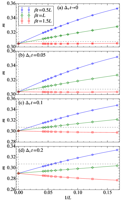
Figure 4: Finite-size scaling of the staggered magnetization $m$ of the half-filled Hubbard model at $U/t=10$ with $\beta t=0.5L,L$, and $1.5L$ for (a) $\Delta_{\tau}t\to 0$, (b) $\Delta_{\tau}t=0.05$, (c) $\Delta_{\tau}t=0.1$, and (d) $\Delta_{\tau}t=0.2$. The dashed horizontal lines indicate $m$ of the Heisenberg model in the thermodynamic limit taken from Ref. Sandvik and Evertz (2010).

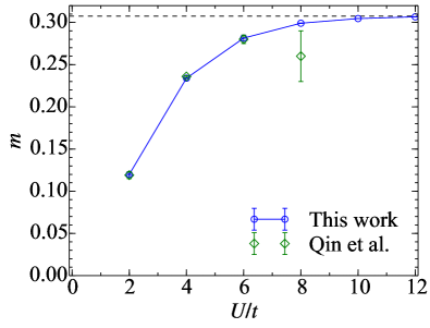
Figure 5: The staggered magnetization $m$ in the thermodynamic limit as a function of $U$. For comparison, previous AFQMC results are taken from Ref. Qin et al. (2016a). The dashed horizontal line indicates $m$ of the Heisenberg model in the thermodynamic limit taken from Ref. Sandvik and Evertz (2010).

V Conclusions and Discussions

In this work we have shown that, within the ground-state AFQMC technique, the choice of the trial function and the one for the auxiliary field are extremely important. In particular we have improved the efficiency of the method, by introducing shifted-discrete HSTs, that are useful for performing the imaginary-time evolution of symmetry-broken trial wave functions. The formalism can be considered as a generalization of the discrete HSTs in Ref. Hirsch (1983) or a compactification of the shifted-contour auxiliary-field Monte Carlo formalism in Ref. Rom et al. (1997, 1998) specialized to the on-site Hubbard interaction.

Properly chosen auxiliary fields can improve the efficiency of AFQMC simulations. The shifted real auxiliary fields can improve the acceptance ratio, while the shifted pure-imaginary auxiliary fields can improve the average sign. The reason is that the shift in the real auxiliary field can stabilize the fluctuations of the norm of the determinant ratio, while the shift in the pure-imaginary auxiliary field can stabilize the fluctuations of the phase of the determinant ratio. However, even after the improvement, the average sign with the pure-imaginary auxiliary field remains worse than the one obtained with real auxiliary field for the doped cases. Therefore, in the presence of the sign problem, the real auxiliary field is still recommended for achieving longer imaginary-time propagations. On the other hand, at half filling with large $U/t$, the pure-imaginary auxiliary field is dramatically more efficient than the real-auxiliary fields for evaluating the staggered magnetization $m$.

In our approach, $m_{i}$ or $n_{i}$ in Eqs. (7) or (16) are arbitrary parameters, that do not have to be necessarily chosen as in Eq. (15) or in Eq. (24). For example, $m_{i}$ ($n_{i}$) can be updated iteratively by the AFQMC expectation value of $\hat{n}_{i\uparrow}-\hat{n}_{i\downarrow}$ ($\hat{n}_{i\uparrow}+\hat{n}_{i\downarrow}$) with iterative simulations. This kind of scheme has already been employed to construct self-consistently an optimized trial wave function in the AFQMC Qin et al. (2016a). Obviously, shifted-discrete HSTs can be used straightforwardly also in this case. Moreover, we expect that imaginary-time dependent $m_{i}$ or $n_{i}$ could further improve the efficiency of the AFQMC, especially within the constrained path formalism. A study along this line is in progress Sorella .

Finally, we remark on the $d$-wave superconducting order which has not been considered in the present study. It is noteworthy that an early study on a $t$-$t^{\prime}$-$J$ model Himeda et al. (2002) has shown that a stripe state with spatially oscillating $d$-wave superconductivity is favored around $1/8$ hole doping. Considering such an inhomogeneous superconductivity in a trial wave function might be of interest for a possible improvement of AFQMC simulations for doped Hubbard models with large $U/t$.

Appendix A Derivation of shifted-discrete HSTs

In this Appendix, we derive Eqs. (10)-(12) and Eqs. (19)-(21). First we derive Eqs. (10)-(12), i.e., the shifted-discrete HST in the spin channel. Since the fermion density operator $\hat{n}_{i\sigma}$ is idempotent, i.e., $\hat{n}_{i\sigma}^{2}=\hat{n}_{i\sigma}$, its exponential function is written as

$$\mathrm{e}^{\alpha s\hat{n}_{\sigma}}=1+\left(\mathrm{e}^{\alpha s}-1\right)\hat{n}_{\sigma},$$ (27)

where, and hereafter, the site index $i$ is dropped for brevity. Then the right-hand side of Eq. (9) is given as

$$\frac{1}{2}\sum_{s=\pm 1}\left[1+\left(\mathrm{e}^{\alpha s}-1\right)\hat{n}_{\uparrow}\right]\left[1+\left(\mathrm{e}^{-\alpha s}-1\right)\hat{n}_{\downarrow}\right]\mathrm{e}^{-s\alpha m}$$ (28)

$$= \cosh{\alpha m}$$

$$+ \left[\cosh{\alpha(1-m)}-\cosh{\alpha m}\right]\ \hat{n}_{\uparrow}$$

$$+ \left[\cosh{\alpha(1+m)}-\cosh{\alpha m}\right]\ \hat{n}_{\downarrow}$$

$$+ \left[2\cosh{\alpha m}-\cosh{\alpha(1-m)}-\cosh{\alpha(1+m)}\right]\hat{n}_{\uparrow}\hat{n}_{\downarrow}.$$

The left-hand side of Eq. (9) is given as

$$C\mathrm{e}^{-\Delta_{\tau}U\tilde{m}^{2}/2}\mathrm{e}^{\frac{\Delta_{\tau}U}{2}(1-2\tilde{m})\hat{n}_{\uparrow}}\mathrm{e}^{\frac{\Delta_{\tau}U}{2}(1+2\tilde{m})\hat{n}_{\downarrow}}\mathrm{e}^{-\Delta_{\tau}U\hat{n}_{\uparrow}\hat{n}_{\downarrow}}$$ (29)

$$= C\mathrm{e}^{-\Delta_{\tau}U\tilde{m}^{2}/2}$$

$$+ C\mathrm{e}^{-\Delta_{\tau}U\tilde{m}^{2}/2}\left[\mathrm{e}^{\frac{\Delta_{\tau}U}{2}(1-2\tilde{m})}-1\right]\hat{n}_{\uparrow}$$

$$+ C\mathrm{e}^{-\Delta_{\tau}U\tilde{m}^{2}/2}\left[\mathrm{e}^{\frac{\Delta_{\tau}U}{2}(1+2\tilde{m})}-1\right]\hat{n}_{\downarrow}$$

$$+ C\mathrm{e}^{-\Delta_{\tau}U\tilde{m}^{2}/2}\left[2-\mathrm{e}^{\frac{\Delta_{\tau}U}{2}(1-2\tilde{m})}-\mathrm{e}^{\frac{\Delta_{\tau}U}{2}(1+2\tilde{m})}\right]\hat{n}_{\uparrow}\hat{n}_{\downarrow}.$$

By comparing Eq. (28) with Eq. (29), we obtain Eqs. (10)-(12).

Next, we derive Eqs. (19)-(21), i.e., the shifted-discrete HST in the charge channel. As in Eq. (27), we have

$$\mathrm{e}^{i\alpha s\hat{n}_{\sigma}}=1+\left(\mathrm{e}^{i\alpha s}-1\right)\hat{n}_{\sigma}.$$ (30)

Then the right-hand side of Eq. (18) is given as

$$\frac{1}{2}\sum_{s=\pm 1}\left[1+\left(\mathrm{e}^{i\alpha s}-1\right)\hat{n}_{\uparrow}\right]\left[1+\left(\mathrm{e}^{i\alpha s}-1\right)\hat{n}_{\downarrow}\right]\mathrm{e}^{-is\alpha n}$$ (31)

$$= \cos{\alpha n}$$

$$+ \left[\cos{\alpha(1-n)}-\cos{\alpha n})\right](\hat{n}_{\uparrow}+\hat{n}_{\downarrow})$$

$$+ \left[\cos{\alpha(2-n)}-2\cos{\alpha(1-n)}+\cos{\alpha n}\right]\hat{n}_{\uparrow}\hat{n}_{\downarrow}.$$

The left-hand side of Eq. (18) is given as

$$C\mathrm{e}^{\Delta_{\tau}U\tilde{n}^{2}/2}\mathrm{e}^{-\frac{\Delta_{\tau}U}{2}(1-2\tilde{n})(\hat{n}_{\uparrow}+\hat{n}_{\downarrow})}\mathrm{e}^{-\Delta_{\tau}U\hat{n}_{\uparrow}\hat{n}_{\downarrow}}$$ (32)

$$= C\mathrm{e}^{\Delta_{\tau}U\tilde{n}^{2}/2}$$

$$+ C\mathrm{e}^{\Delta_{\tau}U\tilde{n}^{2}/2}\left[\mathrm{e}^{-\frac{\Delta_{\tau}U}{2}(1-2\tilde{n})}-1\right]\left(\hat{n}_{\uparrow}+\hat{n}_{\downarrow}\right)$$

$$+ C\mathrm{e}^{\Delta_{\tau}U\tilde{n}^{2}/2}\left[\mathrm{e}^{-\Delta_{\tau}U}\mathrm{e}^{-\Delta_{\tau}U(1-2\tilde{n})}-2\mathrm{e}^{-\frac{\Delta_{\tau}U}{2}(1-2\tilde{n})}+1\right]\hat{n}_{\uparrow}\hat{n}_{\downarrow}.$$

By comparing Eq. (31) with Eq. (32), we obtain Eqs. (19)-(21).

References

- LeBlanc et al. (2015) J. P. F. LeBlanc, A. E. Antipov, F. Becca, I. W. Bulik, G. K.-L. Chan, C.-M. Chung, Y. Deng, M. Ferrero, T. M. Henderson, C. A. Jiménez-Hoyos, E. Kozik, X.-W. Liu, A. J. Millis, N. V. Prokof’ev, M. Qin, G. E. Scuseria, H. Shi, B. V. Svistunov, L. F. Tocchio, I. S. Tupitsyn, S. R. White, S. Zhang, B.-X. Zheng, Z. Zhu, and E. Gull (Simons Collaboration on the Many-Electron Problem), Phys. Rev. X 5, 041041 (2015).
- Zheng et al. (2017) B.-X. Zheng, C.-M. Chung, P. Corboz, G. Ehlers, M.-P. Qin, R. M. Noack, H. Shi, S. R. White, S. Zhang, and G. K.-L. Chan, Science 358, 1155 (2017).
- Sugiyama and Koonin (1986) G. Sugiyama and S. Koonin, Ann. Phys. 168, 1 (1986).
- Sorella et al. (1989) S. Sorella, S. Baroni, R. Car, and M. Parrinello, EPL (Europhysics Letters) 8, 663 (1989).
- Imada and Hatsugai (1989) M. Imada and Y. Hatsugai, Journal of the Physical Society of Japan 58, 3752 (1989).
- Becca and Sorella (2017) F. Becca and S. Sorella, Quantum Monte Carlo Approaches for Correlated Systems (Cambridge University Press, Cambridge, 2017).
- Sorella et al. (2012) S. Sorella, Y. Otsuka, and S. Yunoki, Sci. Rep. 2, 992 (2012).
- Otsuka et al. (2016) Y. Otsuka, S. Yunoki, and S. Sorella, Phys. Rev. X 6, 011029 (2016).
- Otsuka et al. (2018) Y. Otsuka, K. Seki, S. Sorella, and S. Yunoki, Phys. Rev. B 98, 035126 (2018).
- Shi and Zhang (2013) H. Shi and S. Zhang, Phys. Rev. B 88, 125132 (2013).
- Qin et al. (2016a) M. Qin, H. Shi, and S. Zhang, Phys. Rev. B 94, 235119 (2016a).
- Xu et al. (2011) J. Xu, C.-C. Chang, E. J. Walter, and S. Zhang, J. Phys.: Cond. Mat. 23, 505601 (2011).
- Zhang et al. (1997) S. Zhang, J. Carlson, and J. E. Gubernatis, Phys. Rev. B 55, 7464 (1997).
- Zhao et al. (2017) H.-H. Zhao, K. Ido, S. Morita, and M. Imada, Phys. Rev. B 96, 085103 (2017).
- Ido et al. (2018) K. Ido, T. Ohgoe, and M. Imada, Phys. Rev. B 97, 045138 (2018).
- Darmawan et al. (2018) A. S. Darmawan, Y. Nomura, Y. Yamaji, and M. Imada, Phys. Rev. B 98, 205132 (2018).
- Perdew et al. (1995) J. P. Perdew, A. Savin, and K. Burke, Phys. Rev. A 51, 4531 (1995).
- Carrascal et al. (2015) D. J. Carrascal, J. Ferrer, J. C. Smith, and K. Burke, J. Phys.: Cond. Mat. 27, 393001 (2015).
- Tahara and Imada (2008) D. Tahara and M. Imada, J. Phys. Soc. Jpn. 77, 114701 (2008).
- Rodríguez-Guzmán et al. (2012) R. Rodríguez-Guzmán, K. W. Schmid, C. A. Jiménez-Hoyos, and G. E. Scuseria, Phys. Rev. B 85, 245130 (2012).
- Shi et al. (2014) H. Shi, C. A. Jiménez-Hoyos, R. Rodríguez-Guzmán, G. E. Scuseria, and S. Zhang, Phys. Rev. B 89, 125129 (2014).
- Hubbard (1959) J. Hubbard, Phys. Rev. Lett. 3, 77 (1959).
- Hirsch (1983) J. E. Hirsch, Phys. Rev. B 28, 4059 (1983).
- Motome and Imada (1997) Y. Motome and M. Imada, J. Phys. Soc. Jpn. 66, 1872 (1997).
- Held and Vollhardt (1998) K. Held and D. Vollhardt, Eur. Phys. J. B 5, 473 (1998).
- Sakai et al. (2004) S. Sakai, R. Arita, and H. Aoki, Phys. Rev. B 70, 172504 (2004).
- Han (2004) J. E. Han, Phys. Rev. B 70, 054513 (2004).
- Broecker and Trebst (2016) P. Broecker and S. Trebst, Phys. Rev. E 94, 063306 (2016).
- Buividovich and Polikarpov (2012) P. V. Buividovich and M. I. Polikarpov, Phys. Rev. B 86, 245117 (2012).
- Ulybyshev et al. (2013) M. V. Ulybyshev, P. V. Buividovich, M. I. Katsnelson, and M. I. Polikarpov, Phys. Rev. Lett. 111, 056801 (2013).
- Hohenadler et al. (2014) M. Hohenadler, F. Parisen Toldin, I. F. Herbut, and F. F. Assaad, Phys. Rev. B 90, 085146 (2014).
- Tang et al. (2015) H.-K. Tang, E. Laksono, J. N. B. Rodrigues, P. Sengupta, F. F. Assaad, and S. Adam, Phys. Rev. Lett. 115, 186602 (2015).
- Tang et al. (2018) H.-K. Tang, J. N. Leaw, J. N. B. Rodrigues, I. F. Herbut, P. Sengupta, F. F. Assaad, and S. Adam, Science 361, 570 (2018).
- Batrouni and Scalettar (2019) G. G. Batrouni and R. T. Scalettar, Phys. Rev. B 99, 035114 (2019).
- Karakuzu et al. (2018a) S. Karakuzu, K. Seki, and S. Sorella, Phys. Rev. B 98, 201108 (2018a).
- Lieb (1989) E. H. Lieb, Phys. Rev. Lett. 62, 1201 (1989).
- Miyao (2018) T. Miyao, Annales Henri Poincaré 19, 2543 (2018).
- Rom et al. (1997) N. Rom, D. Charutz, and D. Neuhauser, Chem. Phys. Lett. 270, 382 (1997).
- Rom et al. (1998) N. Rom, E. Fattal, A. K. Gupta, E. A. Carter, and D. Neuhauser, The Journal of Chemical Physics 109, 8241 (1998).
- Baer et al. (1998) R. Baer, M. Head-Gordon, and D. Neuhauser, The Journal of Chemical Physics 109, 6219 (1998).
- Zhang and Krakauer (2003) S. Zhang and H. Krakauer, Phys. Rev. Lett. 90, 136401 (2003).
- Motta et al. (2014) M. Motta, D. E. Galli, S. Moroni, and E. Vitali, J. Chem. Phys. 140, 024107 (2014).
- Horn and Weinstein (1984) D. Horn and M. Weinstein, Phys. Rev. D 30, 1256 (1984).
- Weinberg and Sandvik (2017) P. Weinberg and A. W. Sandvik, Phys. Rev. B 96, 054442 (2017).
- Trotter (1959) H. F. Trotter, Proc. Am. Math. Soc. 10, 545 (1959).
- Suzuki (1976) M. Suzuki, Comm. Math. Phys. 51, 183 (1976).
- Hirsch (1985) J. E. Hirsch, Phys. Rev. B 31, 4403 (1985).
- Loh et al. (1990) E. Y. Loh, J. E. Gubernatis, R. T. Scalettar, S. R. White, D. J. Scalapino, and R. L. Sugar, Phys. Rev. B 41, 9301 (1990).
- Qin et al. (2016b) M. Qin, H. Shi, and S. Zhang, Phys. Rev. B 94, 085103 (2016b).
- Karakuzu et al. (2018b) S. Karakuzu, K. Seki, and S. Sorella, Phys. Rev. B 98, 075156 (2018b).
- Hirsch and Tang (1989) J. E. Hirsch and S. Tang, Phys. Rev. Lett. 62, 591 (1989).
- Varney et al. (2009) C. N. Varney, C.-R. Lee, Z. J. Bai, S. Chiesa, M. Jarrell, and R. T. Scalettar, Phys. Rev. B 80, 075116 (2009).
- Assaad and Herbut (2013) F. F. Assaad and I. F. Herbut, Phys. Rev. X 3, 031010 (2013).
- Wang et al. (2014) D. Wang, Y. Li, Z. Cai, Z. Zhou, Y. Wang, and C. Wu, Phys. Rev. Lett. 112, 156403 (2014).
- Anderson (1952) P. W. Anderson, Phys. Rev. 86, 694 (1952).
- Reger and Young (1988) J. D. Reger and A. P. Young, Phys. Rev. B 37, 5978 (1988).
- Sandvik (1997) A. W. Sandvik, Phys. Rev. B 56, 11678 (1997).
- Calandra Buonaura and Sorella (1998) M. Calandra Buonaura and S. Sorella, Phys. Rev. B 57, 11446 (1998).
- Sandvik and Evertz (2010) A. W. Sandvik and H. G. Evertz, Phys. Rev. B 82, 024407 (2010).
- Jiang and Wiese (2011) F.-J. Jiang and U.-J. Wiese, Phys. Rev. B 83, 155120 (2011).
- Sorella (2015) S. Sorella, Phys. Rev. B 91, 241116 (2015).
- Delannoy et al. (2005) J.-Y. P. Delannoy, M. J. P. Gingras, P. C. W. Holdsworth, and A.-M. S. Tremblay, Phys. Rev. B 72, 115114 (2005).
- Gros (1992) C. Gros, Z. Phys. B: Condens. Matter 86, 359 (1992).
- Gros (1996) C. Gros, Phys. Rev. B 53, 6865 (1996).
- Koretsune et al. (2007) T. Koretsune, Y. Motome, and A. Furusaki, J. Phys. Soc. Jpn. 76, 074719 (2007).
- Karakuzu et al. (2017) S. Karakuzu, L. F. Tocchio, S. Sorella, and F. Becca, Phys. Rev. B 96, 205145 (2017).
- (67) S. Sorella, in preparation .
- Himeda et al. (2002) A. Himeda, T. Kato, and M. Ogata, Phys. Rev. Lett. 88, 117001 (2002).