Relationship between Magnetic Field Properties and an X-class Flare in Active Region NOAA 9077

Abstract

The magnetic field plays a key role in producing solar flares, so that the investigation on the relationship between the magnetic field properties and flares is significant. In this paper, based on the magnetic field extrapolated from the photospheric vector magnetograms of the active region NOAA 9077 obtained at Huairou Solar Observing Station, the magnetic field parameters including the height of field lines, force-free factor, free magnetic energy and inclination angle were studied with respect to an X-class flare in this region. We found that the magnetic field lines became lower and the ratio of number of closed field lines to those of open field lines increased after the flare. The force-free factor ($\alpha$) attained a large value before the flare and then decreased after the flare for the closed field lines, while the open field lines showed the opposite tendency. Free energy reach to maximum before flare, then decrease after flare. The magnetic inclination angles showed opposite change trends after the flare for closed and open field lines. Therefore, we may conclude that non-potential energy released by flare mostly contained in the closed magnetic field lines.

1 INTRODUCTION

Solar active region dominated by magnetic field that count for most energetic solar activities such as flare, corona mass ejection and filaments eruption (Krall et al., 1982; Priest & Forbes, 2003; Wiegelmann et al., 2014). Hence, it becomes inevitable to study the relations between magnetic field and flare. Some physical parameters deduced from magnetic field become the targets to investigate the properties of magnetic field and flare (McIntosh, 1990; Lv et al., 1993; Deng et al., 2001; Nindos & Zhang, 2002; Liu et al., 2008). The above researches based on magnetic field observed on the photosphere, the only layer where magnetic field can be measured with high accuracy, as a result the fully understands about magnetic field and flare are limited due to the absence of spatial magnetic field observations on the sun.

The active region space magnetic field can be obtained by magnetic extrapolation assuming field above active region is force-free, which can be regarded a reasonable assumption (Aly, 1989) for low $\beta$ (the ratio of gas pressure to magnetic pressure) plasma circumstances, where magnetic field satisfy $(\nabla\times\textbf{\emph{B}})\times\textbf{\emph{B}}=0$ and $\nabla\cdot\textbf{\emph{B}}=0$. Recently, lots of force-free extrapolation methods are developed and applied to extrapolated chromosphere and corona field (Wu et al., 1990; Mikic et al., 1994; Amari et al., 1997; Sakurai, 1981; Yan & Sakurai, 2000; Wheatland et al., 2000; Wiegelmann, 2004; Song et al., 2006; He & Wang, 2008; Liu et al., 2011a, b). So the tentatively studies about the fully spatial magnetic field and flare become possible basing on magnetic extrapolation (Yan et al., 2001; Wiegelmann et al., 2005; Liu et al., 2011a; Jiang et al., 2013; Liu, 2014; Amari et al., 2014). Then, the studies about magnetic parameters can been deduced from spatial magnetic field become available, which may service to the knowledge of magnetic field and understanding of solar activities.

Solar flares are typical eruption events with its energy comes from magnetic field free energy. It is certain that there exist the changes of magnetic field before and after flares, for kinetic and thermal energy of flare are converted from the magnetic energy. The previous studies have shown some possible changes of magnetic field related parameters before and after solar flare. For example, the increases of transverse magnetic field were found after flare for some active regions (Wang et al., 2005; Su et al., 2012; Wang et al., 2012), there are evident decreases of free energy after the solar flares (Sun et al., 2012). When magnetic field extrapolations are applied to observations, the spatial magnetic field parameters and their relationships with flare are expected to be investigated further.

Systematic observations of the vector magnetic field of active region 9077 from 11 to 15 July were carried out at Huairou Solar Observing Station (HSOS), National Astronomical Observatories of Chinese Academy of Sciences (NAOC). On 14 July 2000, a giant solar flare with an X-ray importance of X5.7 exploded near the disk center in active region 9077. It is one of the greatest solar events in that solar cycle, and the flare caused major terrestrial effects. Based on these high quality vector magnetic field with famous flare event and advanced field extrapolation, it give us a chance to study the spatial magnetic field and it relations with this giant flare. The main targets here is to study spatial field lines distributions, magnetic inclination angles and force-free factor, those magnetic parameters are basically related non-potentiality of active region magnetic field.

This paper is arranged as follows: Section 2 describes the observations data and extrapolation method; in Section 3 the results are given; discussions and conclusions will be given in Section 4.

2 OBSERVATIONS DATA AND EXTRAPOLATION METHOD

The photosphere vector magnetic field used as boundary for extrapolation in this paper is observed by the Solar Magnetic Field Telescope (SMFT) (Ai & Hu, 1986) at HSOS. With SMFT, which is a 35cm solar telescope, the photospheric vector magnetic field can be measured with Fe I $\lambda$ 5324.19 Å. Offset shifted -0.075 Å relative to center of Fe I $\lambda$ 5324.19 Å used to measure the longitudinal magnetic field and the center of line is applied to measure the transverse components. The vector magnetic field is produced by calibrating Stokes parameters ($Q$, $U$ and $V$). $V$ is the difference of the left and right circularly polarized images, $Q$ and $U$ are the differences between two orthogonal linearly polarized images for different azimuthal directions. As for vector magnetic field calibration, series works are carried (Wang et al., 1996; Su & Zhang, 2004), here calibration coefficients of $C_{L}$ and $C_{T}$ are 8381 G and 6790 G are used under the weak-field approximation (Jefferies et al., 1989; Jefferies & Mickey, 1991):

$$B_{L}=C_{L}V,\\$$ (1)

$$B_{T}=C_{T}(Q^{2}+U^{2})^{1/4},\\$$ (2)

$$\theta=arctan(\dfrac{B_{L}}{B_{T}}),\\$$ (3)

$$\phi=\dfrac{1}{2}arctan(\dfrac{U}{Q}),\\$$ (4)

Here, $\theta$ is the inclination between the vector magnetic field and the direction normal to the solar surface and $\phi$ is the field azimuth. Through data processing of SMFT vector magnetic field, the spatial resolution of observational data is about  2^′′/pixel $\times$  2^′′/pixel and noise levels of vector magnetograms are 5 G and 50 G for longitudinal and transverse components, respectively. The observation with the field of view 5.23^′ $\times$ 3.63^′ during this period. The method of minimum energy are employed to resolve $180^{\circ}$ ambiguity, in which both the divergence of the magnetic field ($\nabla\cdot\textbf{\emph{B}}$) and the electric current density ($\textbf{\emph{J}}=\nabla\times\textbf{\emph{B}}$) are minimized simultaneously using a simulated annealing algorithm (Metcalf, 1994; Metcalf et al., 2006). Lastly, the vector magnetic field projected to local heliographic coordinate is used as boundary conditions for magnetic field extrapolation.

The optimization method is used in this paper to extrapolate spatial magnetic field of active region. This method is presented by (Wheatland et al., 2000) and developed by (Wiegelmann, 2004), it consists by minimizing both normalized Lorentz force and the divergence of the field, which is given by the following function,

$$L=\int_{V}\omega(x,y,z)[B^{-2}|(\nabla\times\textbf{B}\times\textbf{B})|^{2}+|\nabla\cdot\textbf{B}|^{2}]d^{3}x,$$ (5)

where $\omega(x,y,z)$ is regarded as a space weighting function. It is undoubt that the force-free conditions can be satisfied when $L$ is equal to zero. This method involves minimizing $L$ by optimizing the solution function $\textbf{B}(x,t)$ through states that are increasingly force- and divergence-free, where $t$ is an artificial time-like parameter introduced in this algorithm.

3 RESULTS

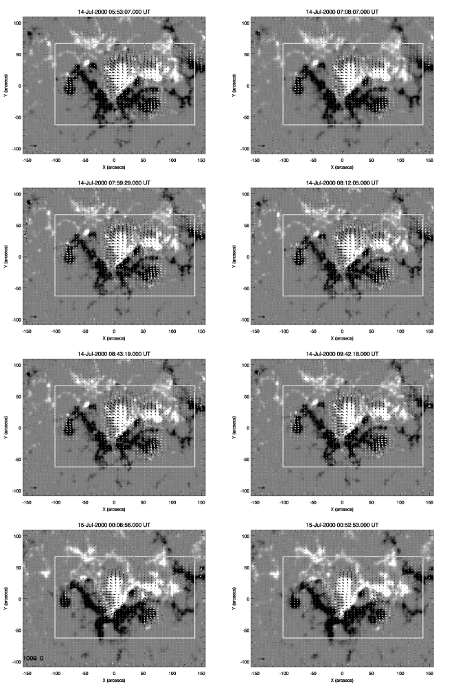
Figure 1: The magnetograms of the observing active region 9077 with the field of view 5.23^′ $\times$ 3.63^′ before and after the flare, times are labelled in each panel respectively. Arrow directions and its length indicate the directions and strength of the transverse field.

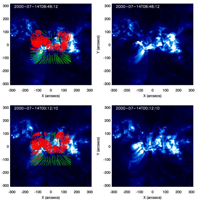
Figure 2: The extrapolated field lines distributions overlaid on the image of EIT/SOHO 195 Å, the red lines are closed and the green ones are open.

Figure 1 shows the vector magnetic fields of the active region observed 9077 before and after the X5.7 flare that erupted at 10:03 on 14 July 2000, the six magnetograms in top three rows were observed before this flare, and the bottom after it. The individual observed time is labelled in each magnetogram. Here, the field of view is 5.23^′ $\times$ 3.63^′, the arrow directions and its length indicate the directions and strength of the transverse fields. The active region can be regarded as a super one (Chen et al., 2011) with evident $\beta\gamma\delta/\beta\gamma\delta$ structures (Maximum area: 1010 $\mu$h), which was accompanied by an Earth-directed coronal mass ejection (CME) and consequently caused major terrestrial effects . The white rectangles in each panel is the region where the magnetic parameters were calculated. Figure 2 shows two examples of the field lines overlaid on the images of EIT/SOHO 195 Å  channel, where red lines are closed in the extrapolation space while the green lines are ones escape the space (here the field of view of EIT are larger than that of extrapolated), it can indicate that most field lines match coronal loops on the whole, so the researches about spatial magnetic field and flare become available basing on extrapolated fields. Figure 3 shows the spatial magnetic field line distributions extrapolated from the magnetic fields of the magnetograms given in Figure 1 as boundary conditions, where the red lines are closed field lines and the blue ones represent open lines, and boxes in green (here the height $\approx$ 66 Mm) correspond to the white rectangles in Figure 1. Here only four cases as examples are shown, the top two panels observed before flare and the lower two after it. On the whole, there are more closed field lines after the flare than those before the flare, by which we were motivated to explore in more detail the information contained in the field extrapolation.

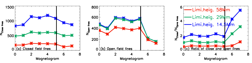
Figure 4: The evolution of the numbers of closed and open field lines, and the ratio of the closed to open lines shown in (a), (b) and (c). The blue, green and red curves indicate the field lines that are higher than 14.5, 29 and 58 Mm, respectively. Here six/two magnetograms observed before/after the flare are calculated. In each panel the vertical lines following the data point based on the sixth magnetogram in fiugre 1 indicates the occurrence of the X5.7 flare.

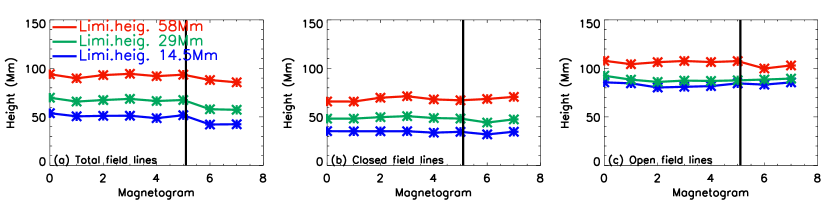
Figure 5: The evolution of the average heights of total lines, closed field lines and the open field lines shown in (a), (b) and (c). The blue, green and red lines indicate the field lines that are higher than 14.5, 29 and 58 Mm are calculated, respectively. Here six/two magnetograms observed before/after the flare are included and calculated. In each panel the vertical lines following the data point based on the sixth magnetogram in fiugre 1 indicates the occurrence of the X5.7 flare.

Figure 4 shows the evolution of the numbers of closed field lines, and open field lines, and the ratio of closed to open field lines. The calculated regions are labelled by green boxes in Figure 2. Blue, green and red curve indicate the height ranges of the field lines are higher than 14.5 (10 pixels), 29 (20 pixels) and 58 (40 pixels) Mm, respectively (the limitations of line heights can be regarded as a threshold). This is done only for relatively larger scale magnetic structures are considered for X5.7 flare, without small scale ones involved temporarily. Six/two magnetograms (corresponding in Figure 1) observed before/after the flare are included and calculated. In each panel in figure 4 the vertical line following the sixth data point indicates the occurrence of the X5.7 flare. To avoid the noise interference, the thresholds of of the observed photospheric longitudinal and transverse fields greater than 20G and 100G respectively are set. In general the closed and open field lines become less after the flare. Additionally, the open field lines decrease faster than closed ones, which results in a sharp increase of the ratio of the number of closed field lines to that of open lines shown in panel (c) in figure 4. Figure 5 shows the evolution of the average heights of the field lines. Same as Figure 3, the calculated heights are higher than 14.5, 29 and 58 Mm shown by blue, green and red curves, respectively, and the thresholds of 20 and 100 G are set for the observed photospheric longitudinal and transverse fields. Panel (a), (b) and (c) represent lines of the total field (the sum of closed and open field lines), closed field lines and open field lines, respectively. On the whole, it can be found that after the flare these relative large scale field lines become lower than those before flare, and this trend is more evident for the lower closed field lines in blue and green shown in (b) in figure 5.

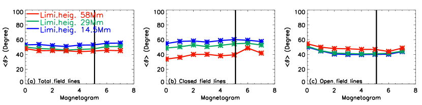
Figure 6: Same as Fig 4, but (a), (b) and (c) showing the evolution of the averages inclinations angles.

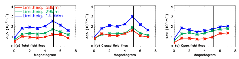
Figure 7: Same as Fig 4, but (a), (b) and (c) showing the evolution of the averages force free factor ($\alpha$).

Figure 6 (a), (b) and (c) show the evolution of average inclination angles ($atan(B_{z},B_{t}),Bt=\sqrt{B^{2}_{x}+B^{2}_{y}}$) calculated from total field lines, closed field lines and open field lines. Same as Figure 3, the calculated heights are higher than 14.5, 29 and 58 Mm shown by blue, green and red curves, respectively, and the thresholds of 20 and 100 G are set for longitudinal and transverse fields. It is shown that in (a) for total field lines are increases in inclination after the flare, especially for field lines at low place. For close field lines (b), at the lower, the inclination decreases after the flare, while at higher height the trend is reverse. Comparing (b) with (c), the changes of inclination of closed and open field lines are opposite, and this trend is consistent at heights. However for individual closed and open field lines distributed at different heights the changes in inclination are different, for example, the changes of red and green(blue) curves in (b) and (c) are different before and after this big flare. Figure 7 shows the evolution of the average force free factor ($\alpha=\nabla\times\textbf{B}/\textbf{B}=\textbf{B}\cdot\nabla\times\textbf{B}/B^{2}$) along the total field lines, closed and open field lines. To take the advantage of the extrapolated spatial magnetic field, the formula $\alpha=\textbf{B}\cdot\nabla\times\textbf{B}/B^{2}$ effectively avoid the singularity of magnetic components of $B_{x}$, $B_{y}$ and $B_{z}$. In Figure 7, after the flare are obvious decrease of $\alpha$ for total field lines and closed field lines, while for open field lines, the values of $\alpha$ evidently increase after the flare. Additionally, the trend of the changes of $\alpha$ in each panel are consistent at various heights. It is also noted that throughout the evolution for total field lines and closed field lines the values of $\alpha$ reach its maxima just before this flare occurs. Free energy (subtract potential magnetic energy from extrapolated NLFF field energy) can been used as a parameter to indicate non-potentiality as $\alpha$, so the evolutions of free energy are shows in the Figure 8, however it is global parameter it can not been divided by open and closed file lines, here we only give it calculated from the whole volume. It can been found that the evolutions of free energy are consistent with those of $\alpha$ calculated from the total field lines and closed ones, it also means that the free energy reach to maximum before flare and decrease evidently after the big flare.

4 Discussions and conclusions

The super solar active region NOAA 9077 with the X5.7 flare is used in this paper to investigate the spatial magnetic field properties, and the changes of the spatial magnetic parameters before and after the flare are focused in this study. The spatial magnetic parameters are deduced from the extrapolated field based on the photospheric magnetic field observed and the force free assumption. The reliability of extrapolated field can be seen by the consistences between extrapolated field line and the EIT loops, they are matched on the whole. The HSOS data adopt linear calibration, so the true magnetic field strength on the sun maybe not very accuracy. However, the topology maybe not depend very strongly on its real strength.

According to the changes of the magnetic field line distribution with height it may be conclude that the reduction of the field lines at higher position after the flare, also implies some of them have vanished. Further as for the decrease of magnetic field lines, the open field lines suffer more than those closed, which leads to the large increase of the ratio of close field lines to open lines after the flare. This may indicate that there are some evident changes in topologies of magnetic field due to a part of open field lines possibly becoming closed after the flare. The change of inclination angles in fact is not so remarkable before and after the big flare. However a rule may be drawn that the direction of inclination changing for closed and open field lines is mostly opposite , and their trends are different at different heights. However, the changes of line number and inclination angles are very faint, it maybe these two parameters are not much sensitive to magnetic field for this event, so there possible exist a strong and reliable effect. Force free factor $\alpha$ deduced from the extrapolated spatial magnetic field shows an interesting pattern before the flare. Even though $\alpha$ decreases for total field line and closed field lines after flare, as for the open field lines there is an increase in $\alpha$ in reverse after flare. Here, force free factor $\alpha$ may be used to scale the extent of non-potentiality of an active region magnetic field indirectly. So the changes of $\alpha$ after flare may mean that the most of flare energy comes from closed field lines, however the open field lines are seriously disturbed by those closed field lines. It should be noted that if some open field lines become closed ones which can also result in the decrease of $\alpha$ of closed field lines , however this effect may not be evident. The decreases of $\alpha$ might be regarded as the release of magnetic free energy (the most parts are contained in the close field lines) to produce a solar flare, and therefore its value reaches maximum just before the flare happens.

It is conventionally regarded that the solar flare energy comes from magnetic field free energy and it may be the outcome of magnetic reconnections. Therefore, when a solar flare occurs, the topology of the magnetic field will be seriously disturbed consequently. Some previous studies based on the photosphere magnetic field have been carried out and results obtained exhibit consistent recognition. In this paper, by means of the advantage of magnetic field extrapolation, the spatial magnetic field is obtained, then the relationships between the spatial magnetic parameters and the flare are expected to receive further confirmation.

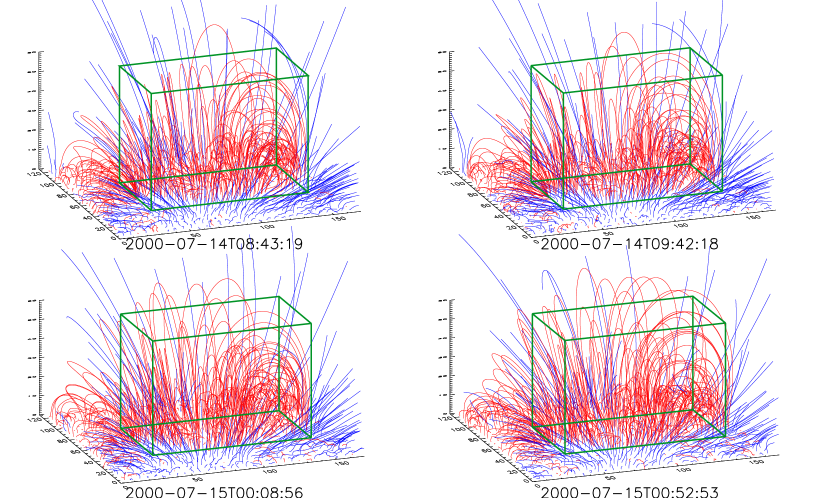
Figure 3: The spatial magnetic field line distributions extrapolated from the magnetic field given in Fig 1. The red lines are closed and the blue represent open lines.

Figure 8: The evolution of magnetic free energy calculated in the whole space extrapolated.

References

- Ai & Hu (1986) Ai, G. & Hu, Y.: 1986, Principles of a solar magnetic field telescope. . , 27, 173,
- Aly (1989) Aly, J.J.: 1989, On the reconstruction of the nonlinear force-free coronal magnetic field from boundary data. Sol. Phys. 120, 19
- Amari et al. (2014) Amari, T., Canou, A. & Aly, J.J.: 2014, Characterizing and predicting the magnetic environment leading to solar eruptions. Nature 514, 465
- Amari et al. (1997) Amari, T., Aly, J.J., Luciani, J.F., Boulmezaoud, T.Z., Mikic, Z.: 1997, Reconstructing the Solar Coronal Magnetic Field as a Force-Free Magnetic Field. Sol. Phys. 174, 129.
- Chen et al. (2011) Chen, A. Q., Wang, J. X., Li, J. W., Feynman, J., Zhang, J. 2011, Statistical properties of superactive regions during solar cycles 19-23. A&A 534, 47.
- Deng et al. (2001) Deng, Y.Y., Wang, J.X., Yan, Y.H. & Zhang, J.: 2001,Evolution of Magnetic Nonpotentiality in NOAA AR 9077. Sol. Phys. 204, 13
- He & Wang (2008) He, H., Wang, H.: 2008, Nonlinear force-free coronal magnetic field extrapolation scheme based on the direct boundary integral formulation. J. Geophys. Res. 113, A05S90
- Jefferies et al. (1989) Jefferies, J., Lites, B.W. & Skumanich, A.: 1989, Transfer of line radiation in a magnetic field. ApJ 343, 920
- Jefferies & Mickey (1991) Jefferies, J., & Mickey, D.L.: 1991, On the inference of magnetic field vectors from Stokes profiles. ApJ 372, 694
- Jiang et al. (2013) Jiang, C.W., Feng, X.S., Wu, S.C. & Hu, Q.: 2013, Magnetohydrodynamic Simulation of a Sigmoid Eruption of Active Region 11283. A&A 771, L30
- Krall et al. (1982) Krall, K. R., Smith, J. B., Jr., Hagyard, M. J., West, E. A. & Cummings, N. P.: 1982, Vector magnetic field evolution, energy storage, and associated photospheric velocity shear within a flare-productive active region. Sol. Phys. 79, 59
- Liu et al. (2008) Liu, J.H. & Zhang, H.Q.: 2008, Relationship between Powerful Flares and Dynamic Evolution of the Magnetic Field at the Solar Surface. Sol. Phys. 248, 67
- Liu et al. (2011a) Liu,S., Zhang, H.Q. & Su, J.T.: 2011, Comparison of Nonlinear Force-Free Field and Potential Field in the Quiet Sun. Sol. Phys. 270, 89
- Liu et al. (2011b) Liu,S., Zhang, H.Q., Su, J.T. & Song, M.T.: 2011, Study on Two Methods for Nonlinear Force-Free Extrapolation Based on Semi-Analytical Field. Sol. Phys. 269, 41
- Liu (2014) Liu,S.: 2014, A statistical study on property of spatial magnetic field for solar active region. Ap&SS 351, 409
- Lv et al. (1993) Lv, Y.P. & Wang, J.X.: 1993, Shear angle of magnetic fields. Sol. Phys. 1485, 119
- Metcalf (1994) Metcalf, T. R.: 1994, Resolving the 180-degree ambiguity in vector magnetic field measurements: The ’minimum’ energy solution. Sol. Phys. 155, 235.
- Metcalf et al. (2006) Metcalf, T. R., Leka, K. D., Barnes, G., Lites, B. W., Georgoulis, M. K., Pevtsov, A. A., Balasubramaniam, K. S., Gary, G. A., Jing, J., & Li, J.: 2006, An Overview of Existing Algorithms for Resolving the 180 Ambiguity in Vector Magnetic Fields: Quantitative Tests with Synthetic Data. Sol. Phys. 237, 267.
- McIntosh (1990) McIntosh, P.S.: 1990, The classification of sunspot groups. Sol. Phys. 125, 251
- Mikic et al. (1994) Mikic, Z.; McClymont, A. N.: 1994, in Solar Active Region Evolution: Comparing Models with Observations, Vol68. ASP Conf. Ser., p.225.
- Nindos & Zhang (2002) Nindos, A. & Zhang, H.Q.: 2002, Photospheric Motions and Coronal Mass Ejection Productivity. ApJ 573, L133
- Priest & Forbes (2003) Priest, E.R. & Forbes, T.G.: 2002, The magnetic nature of solar flares. . 10, 313
- Sakurai (1981) Sakurai, T.: 1981, Calculation of force-free magnetic field with non-constant . Sol. Phys. 69, 343.
- Song et al. (2006) Song, M.T., Fang, C., Tang, Y.H., Wu, S.T., Zhang, Y.A.: 2006,A New and Fast Way to Reconstruct a Nonlinear Force-free Field in the Solar Corona. ApJ 649, 1084.
- Su et al. (2012) Su, J.T., Jing, J., Wang, H. M., Mao, X. J., Wang, X. F., Zhang, H. Q., Deng, Y. Y., Guo, J., Wang, G.P., 2011, ApJ 733, 94
- Su & Zhang (2004) Su, J.T, & Zhang, H.Q.: 2004, Calibration of Vector Magnetogram with the Nonlinear Least-squares Fitting Technique. . . . . 4, 365
- Sun et al. (2012) Sun, X.D., Hoeksema, J.T., Liu, Y., Wiegelmann, T., Hayashi, K., Chen, Q.R. & Thalmann, J.: 2012, Evolution of Magnetic Field and Energy in a Major Eruptive Active Region Based on SDO/HMI Observation. ApJ, 748, 77
- Wang et al. (2005) Wang, H.M., Liu, C., Deng, Y.Y., Zhang, H.Q.: 2005, Reevaluation of the Magnetic Structure and Evolution Associated with the Bastille Day Flare on 2000 July 14. ApJ 627, 1031
- Wang et al. (2012) Wang, S., Liu, C., Liu, R., Deng, N., Liu, Y., Wang, H.M.: 2012, Response of the Photospheric Magnetic Field to the X2.2 Flare on 2011 February 15. ApJ 745, L17
- Wang et al. (1996) Wang T.J., Ai G.X., Deng, Y.Y.: 1996, Calibration of Nine-channel Solar Magnetic field Telescope. I. The methods of the observational calibration. . 23, 31
- Wheatland et al. (2000) Wheatland, M.S., Sturrock, P.A., Roumeliotis, G.: 2000, An Optimization Approach to Reconstructing Force-free Fields. ApJ 540, 1150.
- Wiegelmann (2004) Wiegelmann, T.: 2004, Optimization code with weighting function for the reconstruction of coronal magnetic fields. Sol. Phys. 219, 87.
- Wiegelmann et al. (2005) Wiegelmann, Lagg, A., Solanki, S. K., Inhester, B. & Woch, J.: 2005, Comparing magnetic field extrapolations with measurements of magnetic loops. A&A 433, 701
- Wiegelmann et al. (2014) Wiegelmann, T., Thalmann, J.K. & Solanki, S.K.: 2014,The magnetic field in the solar atmosphere. A&ARv. 22, 78
- Wu et al. (1990) Wu, S.T., Sun, M.T., Chang, H.M., Hagyard, M.J., Gary, G.A.: 1990, On the numerical computation of nonlinear force-free magnetic fields. ApJ 362, 698.
- Yan et al. (2001) Yan, YThe Magnetic Rope Structure and Associated Energetic Processes in the 2000 July 14 Solar Flare. ., Deng, Y.Y., Karlicky, M., Fu, Q.J., Wang, S.J. & Liu, Y.Y.: 2001, Sol. Phys. 551, 115
- Yan & Sakurai (2000) Yan, Y. & Sakurai, T.: 2000, New Boundary Integral Equation Representation for Finite Energy Force-Free Magnetic Fields in Open Space above the Sun. Sol. Phys. 195, 89.