The complexity classes of angular diagrams of the metal conductivity in strong magnetic fields.

Abstract

We consider angular diagrams describing the dependence of the magnetic conductivity of metals on the direction of the magnetic field in rather strong fields. As it can be shown, all angular conductivity diagrams can be divided into a finite number of classes with different complexity. The greatest interest among such diagrams is represented by diagrams with the maximal complexity, which can occur for metals with rather complicated Fermi surfaces. In describing the structure of complex diagrams, in addition to the description of the conductivity itself, the description of the Hall conductivity for different directions of the magnetic field plays very important role. For the evaluation of the complexity of angular diagrams of the conductivity of metals, it is convenient also to compare such diagrams with the full mathematical diagrams that are defined (formally) for the entire dispersion relation.

I Introduction

In this paper, we consider the angular diagrams of the electrical conductivity of metals with arbitrary Fermi surfaces in strong magnetic fields. It is well known that the specific features of the conductivity of metals in this limit are primarily due to specific features of the semiclassical electron trajectories arising on the Fermi surface in the presence of an external magnetic field. More specifically, many nontrivial features in the behavior of conductivity in this case are mainly associated with the appearance of open electron trajectories that appear on Fermi surfaces of a rather complex shape. As a consequence, the complexity of the angular diagrams of conductivity is determined directly by the presence and type of open trajectories appearing on the Fermi surface for different directions of $\,{\bf B}\,$. The angular diagram can then be referred to the “quite complicated” type if it contains regions corresponding to the appearance of open trajectories on the Fermi surface, i.e. the appearance of stable open quasiclassical electron trajectories. This paper will focus mainly on such angular diagrams of conductivity. As it turns out, diagrams of this class can be naturally divided into two types - simpler (type A) and diagrams that can be called ultra-complex (type B) in accordance with their really complicated structure. In this paper, we will describe and compare the complexity of both types of diagrams with the most complex diagrams, namely, diagrams defined for the entire dispersion law. Diagrams of the latter type are somewhat abstract from the point of view of the theory of normal metals; nevertheless, consideration of such diagrams provides a convenient tool for constructing a general approach to the description of diagrams determining the conductivity of normal metals. In particular, consideration of such diagrams allows one to describe the “areas of occurrence” of type A or B diagrams and to estimate the “probability” of the appearance of both types of diagrams for metals with a dispersion law of a given type. Consideration of diagrams defined for the entire dispersion law also makes it possible to naturally include simpler diagrams in the classification, corresponding to the appearance of only closed or unstable open trajectories on the Fermi surface.

Below we give a brief description of the relationship between the behavior of magnetic conductivity and the behavior of semiclassical electron trajectories on the Fermi surface of a metal, which will allow us, in fact, to treat angular diagrams describing the behavior of trajectories on the Fermi surface as conductivity diagrams in strong magnetic fields. In subsequent chapters, we will consider in more detail the structure of the Fermi surface when stable open trajectories appear on it, the features of angular diagrams of conductivity for the entire dispersion law and for a fixed Fermi surface, and compare the structures of the diagrams of both types. As a result of our consideration, we will suggest the general scheme of the natural separation of angular diagrams of conductivity in metals into different classes.

As is well known, electron states in a crystal are parametrized by the values of the quasi-momentum $\,{\bf p}\,=\,(p_{1},p_{2},p_{3})\,$, and any two values of $\,{\bf p}\,$, which differ by a vector of the reciprocal lattice

$${\bf a}\,\,\,=\,\,\,n_{1}{\bf a}_{1}\,\,+\,\,n_{2}{\bf a}_{2}\,\,+\,\,n_{3}{\bf a}_{3}\,\,\,,\quad n_{1},n_{2},n_{3}\,\in\,\mathbb{Z}\,\,\,,$$ (I.1)

specify the same electron state. As is also well known, the basis vectors $\,({\bf a}_{1},{\bf a}_{2},{\bf a}_{3})\,$ of the reciprocal lattice can be chosen in the form

$${\bf a}_{1}\,\,\,=\,\,\,2\pi\hbar\,\,{{\bf l}_{2}\,\times\,{\bf l}_{3}\over({\bf l}_{1},\,{\bf l}_{2},\,{\bf l}_{3})}\,\,\,,\quad\quad{\bf a}_{2}\,\,\,=\,\,\,2\pi\hbar\,\,{{\bf l}_{3}\,\times\,{\bf l}_{1}\over({\bf l}_{1},\,{\bf l}_{2},\,{\bf l}_{3})}\,\,\,,$$

$${\bf a}_{3}\,\,\,=\,\,\,2\pi\hbar\,\,{{\bf l}_{1}\,\times\,{\bf l}_{2}\over({\bf l}_{1},\,{\bf l}_{2},\,{\bf l}_{3})}\,\,\,,$$

where $\,({\bf l}_{1},{\bf l}_{2},{\bf l}_{3})\,$ represent the basis of a direct crystal lattice.

The change in the values of the quasimomentum in the presence of an external constant magnetic field is described by the system (see for example Kittel ; Ziman ; Abrikosov )

$${\dot{\bf p}}\,\,\,\,=\,\,\,\,{e\over c}\,\,\left[{\bf v}_{\rm gr}({\bf p})\,\times\,{\bf B}\right]\,\,\,\,\equiv\,\,\,\,{e\over c}\,\,\left[\nabla\epsilon({\bf p})\,\times\,{\bf B}\right]\,\,\,,$$ (I.2)

where $\,\epsilon({\bf p})\,$ determines the dependence of the electron state energy on the quasi-momentum (dispersion relation) for a fixed conduction band. Due to the fact that any two values of the quasi-momentum that differ by a reciprocal lattice vector specify the same electron state, the function $\,\epsilon({\bf p})\,$ is a 3-periodic function in the $\,{\bf p}$ - space with periods $\,{\bf a}_{1},{\bf a}_{2},{\bf a}_{3}\,$.

The system (I.2) is analytically integrable, in particular, its trajectories in the $\,{\bf p}$ - space are given by the intersections of the surfaces of constant energy $\,\epsilon({\bf p})\,=\,const\,$ with planes orthogonal to $\,{\bf B}\,$. It should be noted here that the description of the geometry of such trajectories for a really complex 3-periodic surface in $\,{\bf p}$ - space is a highly nontrivial problem (see Fig. 1). It is also easy to see that the most complicated is the description of the geometry of open (non-closed) trajectories of (I.2) in the $\,{\bf p}$ - space.

Figure 1: The trajectories of the system (I.2) on a constant energy surface of a rather complicated form.

It is also well known that the trajectories of the system (I.2) in the $\,{\bf p}$ - space correspond to quasiclassical electron trajectories in the coordinate space, which have a somewhat more complicated form (in particular, they are not plane). At the same time, however, the shape of the electron trajectories in the $\,{\bf x}$ - space is in fact closely related to their shape in the $\,{\bf p}$ - space, for example, the projections of the trajectories in the $\,{\bf x}$ - space on the plane orthogonal to $\,{\bf B}\,$ are similar to trajectories in the $\,{\bf p}$ - space, rotated by $90^{\circ}$. The latter property makes the geometry of the trajectories of system (I.2) extremely important for the description of transport phenomena in normal metals in the presence of strong magnetic fields.

The extremely important role of the geometry of the trajectories of the system (I.2) in the description of galvanomagnetic phenomena in normal metals was indicated in the works of the school of I.M. Lifshits in the 1950s (lifazkag ; lifpes1 ; lifpes2 ). During this period, many issues related to the features of electronic phenomena due to the nontrivial geometry of the Fermi surface, in particular, issues related to the geometry of the trajectories of system (I.2), were studied, and many important examples of different types of trajectories on different Fermi surfaces were considered (see for example lifazkag ; lifpes1 ; lifpes2 ; lifkag1 ; lifkag2 ; lifkag3 ; etm ; ElPr ; KaganovPeschansky ; Kittel ; Ziman ; Abrikosov ). We, of course, will not be able to give here even a brief overview of these issues or provide any full bibliography on this topic. In this paper, we will, in fact, be interested in the picture of a complete mathematical description of the structure of the system (I.2), based on the results of the study of this system in a later period. We note here that the shape of the trajectories of (I.2) starts to play a really significant role in the considered phenomena under the condition $\,\omega_{B}\tau\,\gg\,1\,$, where $\,\omega_{B}\,=\,eB/m^{*}c\,$ has the meaning of some effective cyclotron frequency in a crystal and $\,\tau\,$ represents the electron mean free time (lifazkag ).

The problem of complete classification of various types of open trajectories of the system (I.2) with arbitrary (periodic) dispersion laws $\,\epsilon({\bf p})\,$ was set by S.P. Novikov in the 1980s (MultValAnMorseTheory ) and was actively investigated in his topological school in the following decades. It can be said that at present a quite complete description of all types of trajectories of (I.2), based on rather deep mathematical theorems, has been obtained. It should be noted that the most serious breakthroughs in solving this problem were made in zorich1 ; dynn1992 ; dynn1 , where a description of open trajectories of (I.2), which in a certain sense can be called stable open trajectories, was obtained.

We specify here what we shall call open trajectories of the system (I.2) stable if they do not disappear and retain their global geometry under small rotations of the direction of $\,{\bf B}\,$, as well as variations of the energy level $\,\epsilon\,$. As follows from the results of the works zorich1 ; dynn1992 ; dynn1 , the stable open trajectories of the systems (I.2) have the following remarkable properties:

1) Each stable open trajectory of the system (I.2) lies in a straight strip of finite width in the plane orthogonal to $\,{\bf B}\,$, passing it through (Fig. 2);

2) The mean direction of all stable open trajectories in $\,{\bf p}$ - space is the same for a given direction of $\,{\bf B}\,$ and is given by the intersection of the plane orthogonal to $\,{\bf B}\,$ and some integral plane $\,\Gamma\,$, unchanged for small rotations of $\,{\bf B}\,$ and variations of the level $\,\epsilon\,$.

Figure 2: The form of a stable open trajectory of the system (I.2) in the plane orthogonal to $\,{\bf B}\,$.

Properties (1) and (2) of stable open trajectories have direct manifestation in the behavior of galvanomagnetic phenomena in metals in the presence of strong magnetic fields. Namely, the strong anisotropy of the electron trajectories (in $\,{\bf x}\,-\,$ and $\,{\bf p}$ - space) leads to a sharp anisotropy of conductivity in the plane orthogonal to $\,{\bf B}\,$ in the limit $\,\omega_{B}\tau\,\gg\,1\,$. The limiting values of the conductivity tensor in the $\,{\bf x}$ - space can be represented in this situation as

$$\sigma^{kl}_{\infty}\,\,\,\,=\,\,\,\,{ne^{2}\tau\over m^{*}}\,\,\left(\begin{array}[]{ccc}0&0&0\cr 0&*&*\cr 0&*&*\end{array}\right)$$ (I.3)

provided that the $\,x\,$ axis coincides with the mean direction of the stable open trajectories in the $\,{\bf p}$ - space.

It is easy to see that the contribution (I.3) differs significantly from the contribution of closed trajectories in the same limit (see lifazkag )

$$\sigma^{kl}_{\infty}\,\,\,\,=\,\,\,\,{ne^{2}\tau\over m^{*}}\,\,\left(\begin{array}[]{ccc}0&0&0\cr 0&0&0\cr 0&0&*\end{array}\right)$$

(in both formulas, the notation $\,*\,$ represents some dimensionless constant of order 1).

The properties of the tensor (I.3) served as the basis for the introduction in PismaZhETF (see also UFN ) of new topological characteristics (topological quantum numbers) observable in the conductivity of normal metals with complex Fermi surfaces.

Indeed, as is easy to see, the mean direction of stable open trajectories in the $\,{\bf p}$ - space coincides with the direction of the greatest suppression of conductivity in the plane orthogonal to $\,{\bf B}\,$, and, thus, is observable experimentally. Due to the stability of such trajectories, the experimentally observable is actually also the integral plane $\,\Gamma\,$, swept out by the directions of the greatest suppression of conductivity at small rotations of the direction of $\,{\bf B}\,$. The integer parameters of the plane $\,\Gamma\,$ represent in this case the topological quantum numbers observable in conductivity in strong magnetic fields.

We note here that the integerness of the plane $\,\Gamma\,$ means that it is generated by two reciprocal lattice vectors (I.1). In particular, it does not have to coincide in the general case with any of the crystallographic planes; instead, it is orthogonal to some crystallographic direction in the $\,{\bf x}$ - space. Thus, the integral plane $\,\Gamma\,$ observable in the measurements of the magnetic conductivity can be represented by some triple of integers $\,(M^{1},M^{2},M^{3})\,$, specifying some integer direction in the crystal lattice.

Each of the observable topological triples $\,(M_{\alpha}^{1},M_{\alpha}^{2},M_{\alpha}^{3})\,$ is connected with a certain family of stable open trajectories of the system (I.2) corresponding to a certain Stability Zone $\,\Omega_{\alpha}\,$ in the space of directions of $\,{\bf B}\,$ (Fig. 3). As we have said, in the theory of normal metals it is natural to consider the trajectories of the system (I.2) only at one energy level $\,\epsilon({\bf p})=\epsilon_{F}\,$ corresponding to the Fermi energy of a metal. Thus, it is natural to define the boundaries of the Stability Zones $\,\Omega_{\alpha}\,$ for a normal metal by the condition of the existence of open trajectories of the corresponding family on the Fermi surface

$$S_{F}\,:\quad\epsilon({\bf p})\,=\,\epsilon_{F}$$

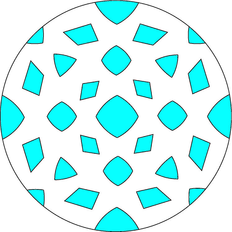
Figure 3: Stability Zones $\,\Omega_{\alpha}\,$ in the space of directions of $\,{\bf B}\,$ corresponding to the appearance of families of stable open trajectories of the system (I.2) with different numbers $\,(M_{\alpha}^{1},M_{\alpha}^{2},M_{\alpha}^{3})\,$ on the Fermi surface.

Note also that the relation (I.3) is true, in particular, also for periodic open trajectories (see lifazkag ), which have rational directions in the $\,{\bf p}$ - space. The latter, however, can both belong to a stable family (if $\,{\bf B}/B\,\in\,\Omega_{\alpha}$), and also be unstable (if $\,{\bf B}/B\,\notin\,\Omega_{\alpha}$).

It must now be said that in addition to stable open trajectories and periodic trajectories of the system (I.2), having a relatively simple form, trajectories with more complicated “chaotic” behavior can also appear on complex enough Fermi surfaces.

The first example of a trajectory of this type was constructed by S.P. Tsarev in 1992 (Tsarev ) for a direction of $\,{\bf B}\,$ of irrationality 2 (the plane orthogonal to $\,{\bf B}\,$ contains a reciprocal lattice vector). Tsarev trajectories can arise on Fermi surfaces of the genus $\,g\geq 3\,$ and have an obvious chaotic behavior on these surfaces. At the same time, in planes orthogonal to $\,{\bf B}\,$ Tsarev-type trajectories have an asymptotic direction and their contribution to conductivity is in fact also strongly anisotropic. In particular, we should also have here the relation (I.3) in the limit $\,\omega_{B}\tau\,\rightarrow\,\infty\,$. On closer examination, however, the contribution of Tsarev’s trajectories to electrical conductivity actually differs from the contributions of stable open or periodic trajectories, which can be revealed in accurate enough experiments. Tsarev-type trajectories are unstable both with respect to small rotations of the direction of $\,{\bf B}\,$, and with respect to variations of the Fermi level.

More complex examples of chaotic trajectories on complex Fermi surfaces are given by trajectories of Dynnikov type (dynn2 ). Dynnikov trajectories can arise only for directions of $\,{\bf B}\,$ of maximal irrationality and possess obvious chaotic behavior both on the Fermi surface and in the covering $\,{\bf p}$ - space (Fig. 4). The main feature of the contribution of such trajectories to the electrical conductivity in this case is a sharp suppression of conductivity along the direction of $\,{\bf B}\,$ in the limit $\,\omega_{B}\tau\,\rightarrow\,\infty\,$ (ZhETF1997 ). In general, the contribution of Dynnikov-type trajectories to the conductivity tensor is characterized by a decrease of conductivity in all directions in the limit $\,\omega_{B}\tau\,\rightarrow\,\infty\,$ and the appearance of fractional powers of the parameter $\,\omega_{B}\tau\,$ in the asymptotics of the tensor components (ZhETF1997 ; TrMian ). Like Tsarev-type trajectories, Dynnikov-type trajectories are unstable both with respect to small rotations of the direction of $\,{\bf B}\,$ and with respect to variations of the Fermi level. As we will see below, the appearance of chaotic trajectories (of both types) will be connected mainly with the most complex angular diagrams (of type B), where the corresponding directions of $\,{\bf B}\,$ will play (together with the Zones $\,\Omega_{\alpha}$) a very important role in the structure of such diagrams.

Figure 4: The form of chaotic trajectories of Dynnikov type in planes orthogonal to $\,{\bf B}\,$ in the $\,{\bf p}$ - space.

As we have said above, in addition to the Stability Zones defined by some fixed Fermi surface, one can in fact also introduce Stability Zones $\,\Omega^{*}_{\alpha}\,$ corresponding to the entire dispersion relation $\,\epsilon({\bf p})\,$ (dynn3 ). The Zones $\,\Omega^{*}_{\alpha}\,$ form, as a rule, a more complex set in the space of directions of $\,{\bf B}\,$ (Fig. 5), in particular, each of the Zones $\,\Omega_{\alpha}\,$ represents a subset of some bigger Zone $\,\Omega^{*}_{\alpha}\,$. In this paper we will discuss the complexity of angular diagrams on $\,\mathbb{S}^{2}\,$ representing the Stability Zones for a fixed Fermi surface, and, in particular, we will make some comparison with the diagrams defined for the whole dispersion law.

Figure 5: Stability Zones $\,\Omega^{*}_{\alpha}\,$ corresponding to the appearance of families of stable open trajectories of the system (I.2) with different numbers $\,(M_{\alpha}^{1},M_{\alpha}^{2},M_{\alpha}^{3})\,$ at least at one of the energy levels $\,\epsilon({\bf p})\,=\,const\,$ (very schematically, only a finite number of Zones is shown).

We also note here that a rather wide range of issues relating to the description of stable trajectories of the system (I.2), both from the point of view of their topological description, and from the point of view of the theory of transport phenomena in metals, was presented in the works DynnBuDA ; JETP1 ; BullBrazMathSoc ; JournStatPhys ; DynSyst ; DeLeoPhysB ; AnProp ; CyclRes ; SecBound .

II Topological representation of the Fermi surface and the Stability Zone in the case of presence of stable open trajectories

In this paper we will focus on Fermi surfaces, which have a rather complex shape. Let us determine at once what we mean by this. First of all, we note the well-known fact that the total space of physical states for a fixed conduction band represents a three-dimensional torus $\,\mathbb{T}^{3}\,$ from the topological point of view. Indeed, by virtue of the above equivalence of states with quasi-momenta differing by the reciprocal lattice vectors, the complete set of states for a given conduction band (Brillouin zone) is a factor space

$$\mathbb{T}^{3}\,\,\,=\,\,\,\mathbb{R}^{3}/L$$

(note also that we do not consider here spin variables that will not play a significant role in our reasoning). As a consequence, any (non-singular) energy surface $\,\epsilon({\bf p})=const\,$ can also be considered (after factorization) as a smooth compact surface embedded into $\,\mathbb{T}^{3}\,$. As a compact smooth two-dimensional surface, each such surface (in particular, the Fermi surface) represents a surface of a certain genus $\,g\geq 0\,$ (Fig. 6).

Figure 6: Topology of closed surfaces of genus 0, 1, 2 (etc.).

In addition to the topological genus, the Fermi surface $\,S_{F}\,$ is also characterized by the rank defined as the dimension of the image of the mapping

$$H_{1}(S_{F})\,\,\,\rightarrow\,\,\,H_{1}(\mathbb{T}^{3})$$

under the embedding $\,S_{F}\,\rightarrow\,\mathbb{T}^{3}\,$. It is easy to see that the rank of the Fermi surface can take the values 0, 1, 2 and 3 (Fig. 7). Let us say at once that we will consider here the Fermi surface rather complicated if its rank is equal to 3. It can be shown that for the genus of the Fermi surface we must in this case also have the relation $\,g\geq 3\,$.

Figure 7: Examples of the Fermi surfaces of rank 0, 1, 2, and 3, respectively.

We now give a brief description of the structure of a complex Fermi surface in the presence of stable open trajectories of the system (I.2). Note that the presence of such a structure is a common property of the system (I.2) and follows from the rigorous topological results presented in the papers zorich1 ; dynn1 ; dynn3 . It will be most convenient for us to use the description presented in the paper dynn3 where all open trajectories of the system (I.2), arising for a given dispersion relation $\,\epsilon({\bf p})\,$, were considered. For simplicity, we will assume here that the Fermi surface is represented by a single connected component having rank 3. Here we will be interested, first of all, in the structure of the Fermi surface for a direction of $\,{\bf B}\,$, lying in one of the Stability Zones $\,\Omega_{\alpha}\,$, for simplicity, we can assume also that $\,{\bf B}\,$ has a generic direction (in particular, the plane orthogonal to $\,{\bf B}\,$ does not contain reciprocal lattice vectors).

Consider, following dynn3 , the set of nonsingular closed trajectories of the system (I.2) with $\,{\bf B}/B\,\in\,\Omega_{\alpha}\,$. It is not difficult to see that this set is a finite set of (nonequivalent) cylinders bounded by singular closed trajectories of the system (I.2) (Fig. 8). We now remove all such cylinders of closed trajectories from the Fermi surface. The remaining part of the Fermi surface is thus a part filled with open trajectories of the system (I.2). It is not difficult to see that the new surface thus obtained should consist of a finite number (nonequivalent) of connected components, which can be called “carriers” of open trajectories. Note also that the holes formed after removing the cylinders of closed trajectories can be “filled” with flat disks orthogonal to $\,{\bf B}\,$, so that a new (reduced) surface can also be viewed as a closed periodic surface in $\,{\bf p}$ - space. The resulting surface can also be factorized by the reciprocal lattice vectors and be considered as a closed two-dimensional surface embedded in $\,\mathbb{T}^{3}\,$.

Figure 8: Cylinder of closed trajectories of (I.2), bounded by singular closed trajectories.

The most important property of the Fermi surface thus reduced in the presence of stable open trajectories of the system (I.2) on it can be formulated as follows (zorich1 ; dynn1 ):

Each of the carriers of open trajectories represents a two-dimensional torus $\,\mathbb{T}^{2}\,$ embedded in $\,\mathbb{T}^{3}\,$ with a fixed mapping in homology uniquely defined for the entire Stability Zone $\,\Omega_{\alpha}\,$.

Coming back to the extended $\,{\bf p}$ - space, we can also formulate the above statement in the form:

Each of the carriers of open trajectories in $\,{\bf p}$ - space represents an integral periodically deformed plane of a given direction, unchanged for the entire Stability Zone $\,\Omega_{\alpha}\,$ (Fig. 9).

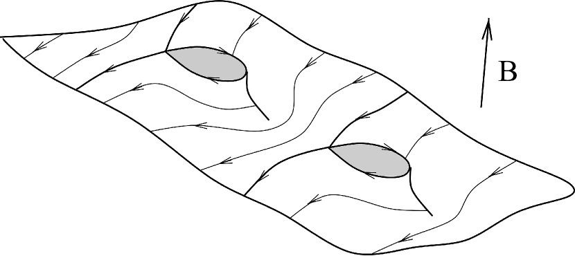
Figure 9: The carrier of stable open trajectories of the system (I.2) in the extended $\,{\bf p}$ - space.

The total reduced Fermi surface thus represents an infinite set of integral periodically deformed parallel planes of a fixed direction in the $\,{\bf p}$ - space. The number of non-equivalent integral planes (that is, representing different electron states) in the reduced Fermi surface is given by a finite even number equal to the number of two-dimensional tori $\,\mathbb{T}^{2}\,$ in the Brillouin zone ($\,\mathbb{T}^{3}\,$).

It can be seen then that for generic directions of $\,{\bf B}\,$ lying in one of the Stability Zones $\,\Omega_{\alpha}\,$ the full Fermi surface is always representable as a set of parallel integral planes (with holes) carrying open trajectories of system (I.2), connected by components consisting only of closed trajectories of (I.2). In our case, we will always assume that such components represent separate cylinders of closed trajectories, bounded by singular closed trajectories (Fig. 10). In fact, more complex structure of these components (consisting of several connected cylinders of closed trajectories with additional singular points) can bring some additional features to the general picture (for example, non-simply-connectedness of Stability Zones). However, such structure is extremely unlikely in a real situation, so we will not consider it here.

Figure 10: Representation of the Fermi surface carrying stable open trajectories of the system (I.2).

The representation of the Fermi surface in the form of Fig. 10 is generally not unique and, in particular, we have different such representations of the same surface for different Stability Zones $\,\Omega_{\alpha}\,$, $\,\Omega_{\beta}\,$. It should also be noted that the representation at Fig. 10 reflects the main features of the topological structure of the system (I.2) on the Fermi surface and can be significantly more complex from a visual point of view.

It is easy to see that the presented structure of the Fermi surface is stable with respect to small rotations of the direction of the magnetic field and explains the remarkable properties of the stable open trajectories of the system (I.2) presented above. It can also be seen that all carriers of open trajectories can actually be divided into two classes according to the direction of motion along the trajectories (forward or backward) in the extended $\,{\bf p}$ - space. In addition, the cylinders of closed trajectories presented at Fig. 10 can also be divided into two classes according to the type of the trajectories (electron or hole) on them.

In accordance with the picture at Fig 10, the boundary of the Stability Zone $\,\Omega_{\alpha}\,$ must necessarily correspond to the vanishing of the height of one of the cylinders of closed trajectories (and its subsequent disappearance) for the corresponding directions of $\,{\bf B}\,$ (Fig. 11). As it is easy to see, after crossing the boundary of a Stability Zone, open trajectories are able to “jump” from one carrier of open trajectories to another, which changes the overall structure of the trajectories on the Fermi surface.

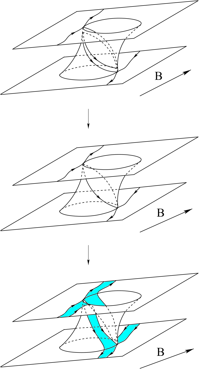
Figure 11: The vanishing of the height of a cylinder of closed trajectories and the subsequent jump of open trajectories from one carrier to another at the boundary of a Stability Zone.

It can also be seen that the full boundary of a Stability Zone can be either “simple”, i.e. correspond to the disappearance of the same cylinder of closed trajectories at all its points (Fig. 12), or “compound”, i.e. correspond to the disappearance of different cylinders of closed trajectories at its different parts (Fig. 13, 14). In addition, it can be seen that in the case of a compound boundary of a Stability Zone we can have both the situation when cylinders of closed trajectories of different types disappear at its different parts (Fig. 13), and also the situation when different cylinders of closed trajectories of the same type disappear at its different parts (Fig. 14).

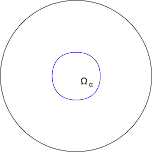
Figure 12: The Fermi surface having a Stability Zone $\,\Omega_{\alpha}\,$ with the boundary defined by the disappearance of the same cylinder of closed trajectories at all its points.

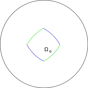
Figure 13: The Fermi surface having a Stability Zone $\,\Omega_{\alpha}\,$ with the boundary defined by the disappearance of different cylinders of different types at different parts of it.

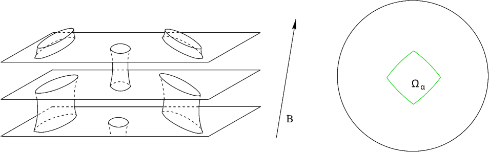
Figure 14: The Fermi surface having a Stability Zone $\,\Omega_{\alpha}\,$ with the boundary defined by the disappearance of different cylinders of the same type at different parts of it.

We note here that the type of vanishing cylinder of closed trajectories also plays an important role in this situation in the description of galvanomagnetic phenomena for the corresponding directions of $\,{\bf B}\,$. Thus, in particular, it determines the value of the Hall conductivity in a metal outside the Zone $\,\Omega_{\alpha}\,$ near the corresponding part of its boundary in the limit $\,\omega_{B}\tau\,\rightarrow\,\infty\,$. As was mentioned in SecBound , the presence of at least one Stability Zone with a compound boundary, determined by the disappearance of cylinders of different types at its different parts, should lead to the presence of different values of Hall conductivity in different areas outside the Stability Zones and, as a result of this, to rather complex structure of the angular diagram as a whole.

III Features of angular diagrams defined for a dispersion law

We now give a general description of the diagrams defined for the entire dispersion law $\,\epsilon({\bf p})\,$ (dynn3 ). According to dynn3 , the possibility of constructing such angular diagrams is based on the following important statements regarding the trajectories of the system (I.2):

1) Consider an arbitrary periodic dispersion relation

$$\epsilon_{min}\,\,\,\leq\,\,\,\epsilon({\bf p})\,\,\,\leq\,\,\,\epsilon_{max}$$

and fix a direction of the magnetic field $\,{\bf B}\,$. Then all energy levels $\,\epsilon({\bf p})=const\,$, at which we have unclosed trajectories of the system (I.2), represent either a closed interval $\,[\epsilon_{1}({\bf B}/B)\,,\,\epsilon_{2}({\bf B}/B)]\,$, or a single point $\,\epsilon_{0}\,=\,\epsilon_{1}({\bf B}/B)\,=\,\epsilon_{2}({\bf B}/B)\,$.

2) For generic directions of $\,{\bf B}\,$ (in particular, directions of maximal irrationality) the values $\,\epsilon_{1}({\bf B}/B)\,$ and $\,\epsilon_{2}({\bf B}/B)\,$ coincide with the values of some continuous functions $\,\tilde{\epsilon}_{1}({\bf B}/B)\,$ and $\,\tilde{\epsilon}_{2}({\bf B}/B)\,$, defined everywhere on the unit sphere. For special directions of $\,{\bf B}\,$, corresponding to the appearance of strictly periodic open trajectories of system (I.2), the values $\,\epsilon_{1}({\bf B}/B)\,$ and $\,\epsilon_{2}({\bf B}/B)\,$ may differ from the values $\,\tilde{\epsilon}_{1}({\bf B}/B)\,$ and $\,\tilde{\epsilon}_{2}({\bf B}/B)\,$ and then we have the relations

$$\epsilon_{1}({\bf B}/B)\,\,\,\leq\,\,\,\tilde{\epsilon}_{1}({\bf B}/B)\,\,\,,\quad\epsilon_{2}({\bf B}/B)\,\,\,\geq\,\,\,\tilde{\epsilon}_{2}({\bf B}/B)$$

3) In the case $\,\tilde{\epsilon}_{2}({\bf B}/B)\,>\,\tilde{\epsilon}_{1}({\bf B}/B)\,$ for generic directions of $\,{\bf B}\,$ all non-singular open trajectories of system (I.2) (at all energy levels) have the form shown at Fig. 2 with the same mean direction defined by the intersection of the plane orthogonal to $\,{\bf B}\,$ and some integral plane $\,\Gamma\,$.

4) The property $\,\tilde{\epsilon}_{2}({\bf B}/B)\,>\,\tilde{\epsilon}_{1}({\bf B}/B)\,$, as well as the integral plane $\,\Gamma\,$, are locally stable with respect to small rotations of $\,{\bf B}\,$ and thus define a certain Stability Zone $\,\Omega^{*}\,$ on the angular diagram. The Zone $\,\Omega^{*}\,$ represents an open domain with a piecewise smooth boundary on $\,\mathbb{S}^{2}\,$ and on the boundary $\,\partial\Omega^{*}\,$ we have the relation $\,\tilde{\epsilon}_{2}({\bf B}/B)\,=\,\tilde{\epsilon}_{1}({\bf B}/B)\,$.

5) The union of all the Stability Zones $\,\Omega^{*}_{\alpha}\,$ is everywhere dense on the unit sphere $\,\mathbb{S}^{2}\,$, and the sphere $\,\mathbb{S}^{2}\,$ can contain either one Stability Zone $\,\Omega^{*}\,$, or infinitely many Zones $\,\Omega^{*}_{\alpha}\,$.

It is easy to see that the angular diagrams for the dispersion law can naturally be divided into very simple (single Stability Zone) and very complex (infinitely many Stability Zones). Here we will be interested mainly in diagrams of the second type. The complexity of the angular diagrams of the second type is due, in particular, to the following features of their general structure (see dynn3 ):

Namely, consider some Stability Zone $\,\Omega^{*}_{\alpha}\,$ corresponding to a certain integral plane $\,\Gamma_{\alpha}\,$ (or topological numbers $\,{\bf M}_{\alpha}\,=\,(M^{1}_{\alpha},M^{2}_{\alpha},M^{3}_{\alpha})$) and having a piecewise smooth boundary on $\,\mathbb{S}^{2}\,$. As already indicated, all non-singular open trajectories of the system (I.2) have at $\,{\bf B}/B\,\in\,\Omega^{*}_{\alpha}\,$ the common mean direction given by the intersection of the plane $\,\Gamma_{\alpha}\,$ and the plane orthogonal to $\,{\bf B}\,$. It is not difficult to see that, whenever such an intersection has an integer direction, the corresponding trajectories are periodic in the $\,{\bf p}$ - space. It can also be seen that the corresponding directions of $\,{\bf B}\,$ form in $\,\Omega^{*}_{\alpha}\,$ an everywhere dense set consisting of segments of the big circles (Fig. 15). In addition, one can see that the corresponding set is also everywhere dense on the boundary of the domain $\,\Omega^{*}_{\alpha}\,$, forming on it a similarity of the set of rational numbers. We will call the points of the described set on the boundary of $\,\Omega^{*}_{\alpha}\,$ “rational” boundary points.

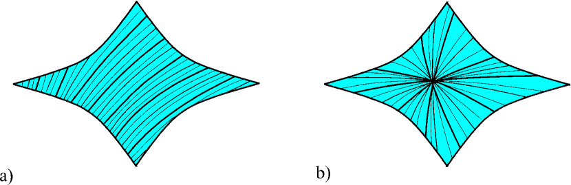
Figure 15: Everywhere dense set of directions of $\,{\bf B}\,$ in the Zone $\,\Omega^{*}_{\alpha}\,$, corresponding to the appearance of periodic trajectories, in the cases when $\,{\bf M}_{\alpha}/|{\bf M}_{\alpha}|\,\notin\,\Omega^{*}_{\alpha}\,$ and $\,{\bf M}_{\beta}/|{\bf M}_{\beta}|\,\in\,\Omega^{*}_{\alpha}\,$.

An important feature of angular diagrams for the dispersion law is the fact that at each “rational” point of the boundary of any of the Stability Zones $\,\Omega^{*}_{\alpha}\,$ another Stability Zone $\,\Omega^{*}_{\beta}\,$, corresponding to another integral plane $\,\Gamma_{\beta}\,$, is adjacent to this Zone (Fig. 16). The corresponding junction point represents a corner point of the boundary of $\,\Omega^{*}_{\beta}\,$, and the topological numbers $\,{\bf M}_{\alpha}\,=\,(M^{1}_{\alpha},M^{2}_{\alpha},M^{3}_{\alpha})\,$ and $\,{\bf M}_{\beta}\,=\,(M^{1}_{\beta},M^{2}_{\beta},M^{3}_{\beta})\,$, as well as the corresponding direction of $\,{\bf B}\,$, are connected by the relation

$${\bf B}\,\,\,=\,\,\,\eta\,{\bf M}_{\alpha}\,\,+\,\,\theta\,{\bf M}_{\beta}\,\,\,,$$

where $\,|\eta/\theta|\,<\,1\,$.

Figure 16: The set of Zones $\,\Omega^{*}_{\beta}\,$ adjoining the boundary of a Zone $\,\Omega^{*}_{\alpha}\,$ at each of its “rational” points.

It can be seen, therefore, that the structure of the angular diagrams for the dispersion relation, containing more than one Stability Zone, is extremely complex.

To avoid ambiguity, we will always denote here by $\,\Omega^{*}_{\alpha}\,$ a complete (open) Stability Zone and by $\,{\overline{\Omega^{*}_{\alpha}}}\,$ - the Zone $\,\Omega^{*}_{\alpha}\,$ together with the boundary. The set

$${\cal D}^{*}\,\,\,=\,\,\,\mathbb{S}^{2}\,\left\backslash\,\cup\,{\overline{\Omega^{*}_{\alpha}}}\right.$$

represents the set of directions of $\,{\bf B}\,$, for which open trajectories of the system (I.2) exist on a single energy level and have generically a chaotic behavior in planes orthogonal to $\,{\bf B}\,$. According to the conjecture of S.P. Novikov (see DynSyst ), the fractal dimension of this set for generic dispersion relations is strictly less than 2. We note here that the study of various features of both the set $\,{\cal D}^{*}\,$ and the corresponding chaotic trajectories of (I.2) is currently a rapidly developing area of the theory of dynamical systems (see for example Tsarev ; dynn2 ; dynn3 ; zorich2 ; Zorich1996 ; ZorichAMS1997 ; ZhETF1997 ; zorich3 ; DeLeo1 ; DeLeo2 ; DeLeo3 ; ZorichLesHouches ; DeLeoDynnikov1 ; DeLeoDynnikov2 ; Skripchenko1 ; Skripchenko2 ; DynnSkrip1 ; DynnSkrip2 ; AvilaHubSkrip1 ; AvilaHubSkrip2 ; DeLeo2017 ; TrMian ).

The above description of the angle diagrams for system (I.2), built in dynn3 , is based on the results obtained in the works zorich1 ; dynn1 and leading to the above-described representation of the energy surfaces (Fig. 10) containing stable open trajectories of system (I.2). Note here also that the boundary of a Stability Zone $\,\Omega^{*}_{\alpha}\,$, defined for the entire dispersion law, corresponds to the simultaneous disappearance of two cylinders of closed trajectories (of electron and hole type) connecting the carriers of open trajectories. Here one can see the difference with the situation on the angular diagrams defined for a fixed value of energy, where each segment of the boundary of a Stability Zone corresponds to the disappearance of a cylinder of closed trajectories of a certain type. In addition, as was noted in dynn3 , the boundaries of different Stability Zones defined for a fixed energy value have no common points in the generic case, which indicates in general a somewhat less complex structure of such diagrams.

In the next chapter, we will give a more detailed consideration of angular diagrams of conductivity corresponding to some fixed energy level (Fermi level) $\,\epsilon_{F}\,$, which corresponds to the situation of a normal metal. As we will see, most of the consideration will need to be devoted to the study of the trajectories of system (I.2) on the complex Fermi surfaces discussed in the previous chapter. This study will, in particular, contain a description of the most complex diagrams that arise in this situation and the investigation of how such diagrams can approach those described above in terms of complexity.

IV The complexity of the angular diagrams defined for a fixed Fermi surface, and their relation to the diagrams for the dispersion law

As we indicated above, each of the Stability Zones $\,\Omega_{\alpha}\,$, defined for a fixed Fermi surface, lies inside some (larger) Stability Zone $\,\Omega^{*}_{\alpha}\,$, corresponding to the full dispersion relation $\,\epsilon({\bf p})\,$. For directions $\,{\bf B}/B\,\in\,\Omega_{\alpha}\,$ we thus have stable open trajectories lying on the Fermi surface and corresponding to topological numbers $\,(M^{1}_{\alpha},M^{2}_{\alpha},M^{3}_{\alpha})\,$.

We note here at once one feature of the Stability Zones for a fixed Fermi surface, which somewhat distinguishes them from the Stability Zones for the entire dispersion law. As we have already said, the Stability Zone $\,\Omega_{\alpha}\,$ defines a set of directions of $\,{\bf B}\,$, for which there exist stable open trajectories on the Fermi surface corresponding to fixed topological numbers $\,(M^{1}_{\alpha},M^{2}_{\alpha},M^{3}_{\alpha})\,$. We can, however, specify additional directions of $\,{\bf B}\,$, for which there are open trajectories of the system (I.2) on the Fermi surface that are not stable but are also associated with the Zone $\,\Omega_{\alpha}\,$. Such trajectories are periodic and appear on the continuations of the segments of large circles described above, beyond $\,\Omega_{\alpha}\,$ (Fig. 17). It can be shown that such trajectories always appear near the boundary of a Zone $\,\Omega_{\alpha}\,$, which follows from the above representation of the Fermi surface (Fig. 10) for directions $\,{\bf B}/B\,\in\,\Omega_{\alpha}\,$. The net of the corresponding directions of $\,{\bf B}\,$ is everywhere dense on the boundary of $\,\Omega_{\alpha}\,$, however, the lengths of the additional segments of the large circles decrease rapidly with increasing of the integers $\,(m_{1},m_{2},m_{3})\,$, which determine the direction of the corresponding periodic trajectories in the $\,{\bf p}$ - space. As a consequence, the described nets of additional directions of $\,{\bf B}\,$ have a finite density at any finite distance from the boundary of $\,\Omega_{\alpha}\,$. As was shown in AnProp , the presence of (unstable) periodic trajectories, as well as very long closed trajectories of system (I.2) near the boundaries of $\,\Omega_{\alpha}\,$ actually leads to rather complex conductivity behavior for the corresponding directions of $\,{\bf B}\,$ and, in particular, makes impossible the observation of the exact boundary of a Stability Zone in direct measurements of conductivity even in rather strong magnetic fields. So, in reality, the “experimentally observed” Stability Zone in such experiments does not coincide with the exact mathematical Zone $\,\Omega_{\alpha}\,$ (Fig. 18) and depends on the maximal values of external magnetic fields reachable in the experiment.

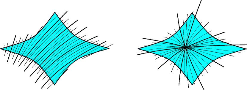
Figure 17: The set of directions of $\,{\bf B}\,$ near Stability Zones, corresponding to the appearance of (unstable) periodic trajectories on the Fermi surface.

Figure 18: “Experimentally observable” Stability Zones in experiments on direct measurements of conductivity in strong magnetic fields.

At the same time, the exact boundaries of the mathematical Stability Zones $\,\Omega_{\alpha}\,$ are in fact also observable experimentally with a special experimental setup. In particular, as was shown in CyclRes , they can be determined by observing the picture of oscillation phenomena (classical or quantum) in strong magnetic fields. In this paper, we will be interested in the distribution of precisely exact mathematical Stability Zones on an angular diagram of conductivity.

As can be seen from the above picture, which appears on the Fermi surface in the case of presence of stable open trajectories of the system (I.2), for each of the Stability Zones $\,\Omega_{\alpha}\,$ it is also natural to introduce the “second boundary” on the angular diagram. The second boundary of the Zone $\,\Omega_{\alpha}\,$ is determined by the disappearance of one more cylinder of closed trajectories at Fig. 10 and the appearance of jumps of trajectories of (I.2) between pairs of “merged” carriers of open trajectories defined for the Zone $\,\Omega_{\alpha}\,$. It can be seen that in the region $\,\Omega^{\prime}_{\alpha}\,$, which lies between the first and second boundaries of the Stability Zone, there can not be open trajectories of the system (I.2), other than the unstable periodic trajectories described above. The domain $\,\Omega^{\prime}_{\alpha}\,$ can be called the “derivative” of the Stability Zone $\,\Omega_{\alpha}\,$, since the behavior of trajectories of the system (I.2) in this area is actually determined by the structure of this system in the Zone $\,\Omega_{\alpha}\,$. We note here that the picture of the behavior of conductivity, as well as the oscillation phenomena, in the region $\,\Omega^{\prime}_{\alpha}\,$ is, in general, rather complicated (see SecBound ). As well as for the first boundary of a Stability Zone $\,\Omega_{\alpha}\,$, the position of its second boundary is also most convenient to determine with the help of the study of oscillation phenomena in strong magnetic fields (SecBound ).

As can be seen, in the general case, the second boundary of a Stability Zone can be located at an arbitrary distance from its first boundary. In the general case, the domain $\,\Omega^{\prime}_{\alpha}\,$ may consist of several connected components bounded by parts of the first boundary of the Zone $\,\Omega_{\alpha}\,$ from the “internal” side and by parts of the second boundary from the “external” side (Fig. 19). It can also be noted that for each of the connected components of the domain $\,\Omega^{\prime}_{\alpha}\,$ its “internal” and “external” boundaries correspond to the disappearance of cylinders of closed trajectories of opposite types at Fig. 10. Within each domain $\,\Omega^{\prime}_{\alpha}\,$ there is also the boundary of the Stability Zone $\,\Omega^{*}_{\alpha}\,$, which has both the “electron” and the “hole” type (Fig. 20). It is also a common circumstance that for a Stability Zone with a compound boundary that has sections corresponding to the disappearance of cylinders of closed trajectories of different types, the “corner” points of its boundaries (separating sections corresponding to the disappearance of cylinders of closed trajectories of different types) are also “corner” points for the second boundary of the Stability Zone, and also belong to the boundary of the corresponding Zone $\,\Omega^{*}_{\alpha}\,$ (Fig. 20, b). At the same time, for a Stability Zone, whose boundaries completely correspond to the disappearance of cylinders of closed trajectories of the same type, its first boundary does not intersect the second boundary in the generic case, and the boundary of the corresponding Zone $\,\Omega^{*}_{\alpha}\,$ lies inside the area bounded by the first and second boundaries (Fig. 20, a, c).

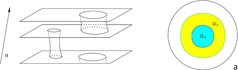
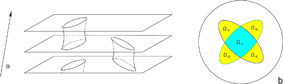
Figure 19: Internal and external boundaries bounding the domains $\,\Omega^{\prime}_{\alpha}\,$.

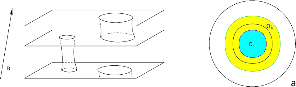
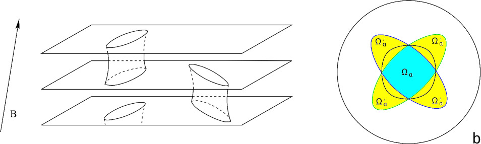
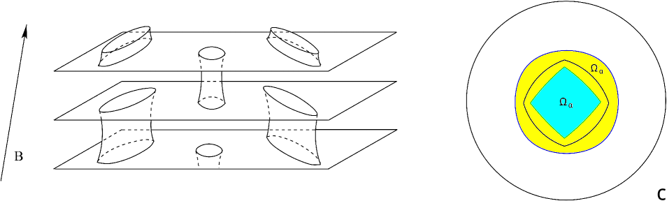
Figure 20: The boundaries of the Zones $\,\Omega^{*}_{\alpha}\,$ inside the domains $\,\Omega^{\prime}_{\alpha}\,$.

It will be convenient for us here to introduce some special notations for different types of Zones $\,\Omega_{\alpha}\,$. Namely, let’s say that the Zone $\,\Omega_{\alpha}\,$ is of type $(+)$ if all points of its boundary correspond to the disappearance of cylinders of closed electron-type trajectories. Similarly, let’s say that $\,\Omega_{\alpha}\,$ is of type $(-)$ if all points of its boundary correspond to the disappearance of cylinders of closed hole-type trajectories. Finally, the Zone $\,\Omega_{\alpha}\,$ is of the type $(\pm)$ if at different parts of its boundary the cylinders of closed trajectories of both the electron and hole type disappear.

It is not difficult to show that on the sections of the boundaries of $\,\Omega_{\alpha}\,$ corresponding to the disappearance of cylinders of closed electron-type trajectories we have in generic case the relation

$$\epsilon_{F}\,\,\,=\,\,\,\tilde{\epsilon}_{2}({\bf B}/B)\,\,\,>\,\,\,\tilde{\epsilon}_{1}({\bf B}/B)$$

Similarly, on the sections of the boundaries of $\,\Omega_{\alpha}\,$ corresponding to the disappearance of cylinders of closed hole-type trajectories we have in generic case the relation

$$\epsilon_{F}\,\,\,=\,\,\,\tilde{\epsilon}_{1}({\bf B}/B)\,\,\,<\,\,\,\tilde{\epsilon}_{2}({\bf B}/B)$$

A special situation takes place at the “corner” (separating parts of the boundary of different types) points of the Zones of type $(\pm)$, where we have the relation

$$\epsilon_{F}\,\,\,=\,\,\,\tilde{\epsilon}_{1}({\bf B}/B)\,\,\,=\,\,\,\tilde{\epsilon}_{2}({\bf B}/B)$$

It can be seen here that for a generic Fermi surface all the Stability Zones $\,\Omega_{\alpha}\,$ of type $(+)$ can be covered with open domains $\,U^{+}_{\alpha}\,$, and the Stability Zones $\,\Omega_{\beta}\,$ of type $(-)$ - with open domains $\,U^{-}_{\beta}\,$, such that:

1) All domains $\,U^{+}_{\alpha}\,$ and $\,U^{-}_{\beta}\,$ do not intersect with each other, as well as with the Stability Zones $\,\Omega_{\alpha}\,$ of type $(\pm)$;

2) Everywhere on the sets $\,U^{+}_{\alpha}\,\backslash\,\overline{\Omega_{\alpha}}\,$ takes place the relation

$$\epsilon_{F}\,\,\,>\,\,\,\tilde{\epsilon}_{2}({\bf B}/B)\,\,\,,$$ (IV.1)

and on the sets $\,U^{-}_{\beta}\,\backslash\,\overline{\Omega_{\beta}}\,$ - the relation

$$\epsilon_{F}\,\,\,<\,\,\,\tilde{\epsilon}_{1}({\bf B}/B)$$ (IV.2)

Coming back to the full dispersion relation, it can be noted that each Zone $\,\Omega_{\alpha}\,$ passes in generic case all types $\,(-)$ , $\,(\pm)\,$ and $\,(+)\,$ when the Fermi level changes from some minimal to some maximal value, determined by the existence of this Zone. Fig. 21 presents a possible scheme of the evolution of a Zone $\,\Omega_{\alpha}\,$ when changing $\,\epsilon_{F}\,$ in the interval $\,[\epsilon_{min},\epsilon_{max}]\,$.

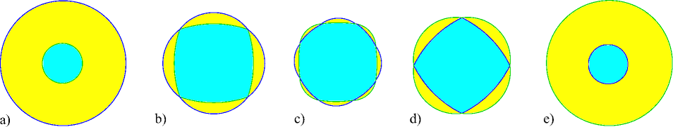
Figure 21: Change of the shape of the Zones $\,\Omega_{\alpha}\,$ and $\,\Omega^{\prime}_{\alpha}\,$ with increasing the value of $\,\epsilon_{F}\,$ for a fixed dispersion relation $\,\epsilon({\bf p})\,$. (a) The appearance and growth of a Stability Zone $\,\Omega_{\alpha}\,$ having the type $(-)$. (b) The connection of the first and second boundaries of the Zone $\,\Omega_{\alpha}\,$ and the formation of a Zone of type $(\pm)$. (c) Evolution of the Zone of type $(\pm)$. (d) Change of type to $(+)$. (e) Decrease and disappearance of a Zone of Type $(+)$.

As we have already said, we will be interested here in the questions of the complexity of angular diagrams for conductivity in metals with arbitrary (physical) dispersion relations. We also note here that in the work SecBound it was proposed to divide all non-trivial (containing Stability Zones) angular diagrams of metals into simpler (type A) and more complex (type B). As noted in SecBound , these features of angular diagrams are related to the behavior of the Hall conductivity outside the Stability Zones in the limit $\,\omega_{B}\tau\,\rightarrow\,\infty\,$.

More precisely, for generic directions of $\,{\bf B}\,$, lying outside any Stability Zone, on the Fermi surface there exist only closed trajectories of the system (I.2). The conductivity tensor in the plane orthogonal to $\,{\bf B}\,$ can be represented in this case as a regular series in inverse powers of the parameter $\,\omega_{B}\tau\,$ in the limit $\,\omega_{B}\tau\,\rightarrow\,\infty\,$ and has in the main order the following form

$$\sigma^{\alpha\beta}\,\,\,=\,\,\,\left(\begin{array}[]{cc}a^{11}\,(\omega_{B}\tau)^{-2}&\,a^{12}\,(\omega_{B}\tau)^{-1}\cr-a^{12}\,(\omega_{B}\tau)^{-1}&\,a^{22}\,(\omega_{B}\tau)^{-2}\end{array}\right)\,\,,\\ \omega_{B}\tau\,\rightarrow\,\infty$$ (IV.3)

The value $\,\sigma^{12}\,=\,a^{12}(\omega_{B}\tau)^{-1}\,$ can be in this case represented as

$$\sigma^{12}\,\,\,=\,\,\,{ec\over B}\,\left(n_{e}-n_{h}\right)\,\,\,,$$ (IV.4)

where the values $\,n_{e}\,$ and $\,n_{h}\,$ represent the “electrons” and “holes” concentration for a given direction of $\,{\bf B}\,$. The values $\,n_{e}\,$ and $\,n_{h}\,$ can be defined by the formulae

$$n_{e}\,\,\,=\,\,\,2V_{e}/(2\pi\hbar)^{3}\quad,\quad\quad n_{h}\,\,\,=\,\,\,2V_{h}/(2\pi\hbar)^{3}\,\,\,,$$

where $\,V_{e}\,$ and $\,V_{h}\,$ represent the volumes bounded by all nonequivalent cylinders of closed trajectories (on the Fermi surface) of the electron and hole type in $\,{\bf p}$ - space.

An important feature of the picture arising for generic directions of $\,{\bf B}\,$, lying outside any Stability Zone, is that in all planes orthogonal to $\,{\bf B}\,$ we have the same type of the behavior of trajectories of system (I.2), determined by one of the following possibilities:

I) The region of the higher energy values $\,\epsilon({\bf p})\,>\,\epsilon_{F}\,$ represents the “sea” in the plane orthogonal to $\,{\bf B}\,$, while the areas of the lower energy values $\,\epsilon({\bf p})\,<\,\epsilon_{F}\,$ represent finite “islands” (“islands” may contain “lakes” of higher energy values, etc., Fig. 22, a).

II) The region of the lower values of energy $\,\epsilon({\bf p})\,<\,\epsilon_{F}\,$ represents the “sea” in the plane orthogonal to $\,{\bf B}\,$, while the areas of the higher energy values $\,\epsilon({\bf p})\,>\,\epsilon_{F}\,$ represent finite “islands” (“islands” may contain “lakes” of lower energy values, etc., Fig. 22, b).

Figure 22: Two possible pictures in planes orthogonal to $\,{\bf B}\,$ in the case when the Fermi surface contains only closed trajectories in the $\,{\bf p}$ - space.

As a consequence of the picture described above, the value of $\,\sigma^{12}\,$ in this case is actually determined by one of the following relations:

$$\sigma^{12}\,\,\,=\,\,\,{2ec\over(2\pi\hbar)^{3}B}\,\,\,V_{-}\quad\quad{\rm(\text{case I})}$$ (IV.5)

$$\sigma^{12}\,\,\,=\,\,\,-\,{2ec\over(2\pi\hbar)^{3}B}\,\,\,V_{+}\quad\quad{\rm(\text{case II})}$$ (IV.6)

where $\,V_{-}\,$ and $\,V_{+}\,$ represent the volumes, defined by the conditions $\,\epsilon({\bf p})\,<\,\epsilon_{F}\,$ and $\,\epsilon({\bf p})\,>\,\epsilon_{F}\,$ in the Brillouin zone.

As a result, the magnitude of the Hall conductivity is locally constant (at a constant value of $\,B$) everywhere outside the Stability Zones under the condition $\,\omega_{B}\tau\,\gg\,1\,$. (In fact, the condition $\,\tau\,\gg\,T\,$, where $\,T\,$ is typical time of electron motion along a closed trajectory for a given direction of $\,{\bf B}\,$. As was noted in SecBound , this condition may be stronger.) This circumstance, as is easy to see, gives a simple tool of experimental determination of each of the two described situations for directions of $\,{\bf B}\,$ lying outside the Stability Zones. In this case, the areas corresponding to different situations described above should be separated by Stability Zones, which in the generic case form “chains” consisting of an infinite number of Zones.

Let us define the type (A or B) of the angular diagram of conductivity of metal as follows:

We say that the angular diagram of the conductivity of a metal is of type A, if for all generic directions of $\,{\bf B}\,$ outside the Zones $\,\overline{\Omega_{\alpha}}\,$ we observe only one type of the Hall conductivity in the limit $\,\omega_{B}\tau\,\rightarrow\,\infty\,$. We say that the angular diagram of the conductivity of a metal is of type B, if for different generic directions of $\,{\bf B}\,$ outside the Zones $\,\overline{\Omega_{\alpha}}\,$ both types of the Hall conductivity can be observed in the limit $\,\omega_{B}\tau\,\rightarrow\,\infty\,$.

Let us make here one more remark concerning the Fermi surfaces of real metals. As we have said above, we assume here for simplicity that the Fermi surface consists of one connected component, on which we consider the trajectories of the system (I.2). In fact, the Fermi surface of a real metal usually consists of several components and very often contains components of the genus 0 or 1 along with complex components. In calculating the Hall conductivity, we must in fact add up the contributions from all components of the Fermi surface, which also have the properties described above. In this case, it may turn out that the type of total Hall conductivity may differ from the type of contribution to this conductivity from the component we are considering. Therefore, it would be more strict to say that the angular diagram of the conductivity of a metal is of type A, if for all generic directions of $\,{\bf B}\,$ outside the Zones $\,\overline{\Omega_{\alpha}}\,$ there is only one value of the Hall conductivity (for a given value of $\,B$) under the condition $\,\omega_{B}\tau\,\gg\,1\,$, and the angular diagram of the conductivity of a metal is of type B, if for different generic directions of $\,{\bf B}\,$ outside the Zones $\,\overline{\Omega_{\alpha}}\,$ at least two values of the Hall conductivity can be observed under the same condition. We will, however, keep here the terminology introduced above for greater transparency of the presentation.

As was also noted in SecBound , an angular diagram has type B, in particular, if it contains at least one Stability Zone of type $(\pm)$. Indeed, as can be shown (see SecBound ), in different connected components of the corresponding domain $\,\Omega^{\prime}_{\alpha}\,$ there present in this case different types of the Hall conductivity for generic directions of $\,{\bf B}\,$ (Fig. 23). It can be seen that in this situation a chain of Stability Zones should adjoin the “corner point” of $\,\Omega_{\alpha}\,$, separating regions with different Hall conductivity that appear near the corresponding sections of the boundary of $\,\Omega_{\alpha}\,$. In this case, the Zone $\,\Omega_{\beta}\,$ can adjoin directly to the “corner point” of $\,\Omega_{\alpha}\,$ only if the corresponding direction of $\,{\bf B}\,$ corresponds to the appearance of periodic trajectories (with the direction given by the intersection of the planes $\,\Gamma_{\alpha}$ and $\,\Gamma_{\beta}\,$) on the Fermi surface, which corresponds to a non-generic situation. In the generic case, a chain of an infinite number of decreasing Stability Zones $\,\Omega_{\beta}\,$ should adjoin the “corner point” of $\,\Omega_{\alpha}\,$ (Fig. 23).

Figure 23: Regions with different values of Hall conductivity and a chain of decreasing Stability Zones and “chaotic” directions of $\,{\bf B}\,$ near the “corner point” of the boundary of a Stability Zone of type $(\pm)$.

Let us note here that accumulation points of decreasing Stability Zones, which are not boundary points of Stability Zones, represent generically directions of $\,{\bf B}\,$ corresponding to the appearance of chaotic trajectories (of Tsarev or Dynnikov type) on the Fermi surface. The set of the corresponding directions of $\,{\bf B}\,$ represents in the general case a rather complex set on the angular diagram. As can be shown (see dynn3 ), the full measure of such directions on the angular diagram is zero for a generic Fermi surface. According to the conjecture of S.P. Novikov (BullBrazMathSoc ; JournStatPhys ), the fractal dimension of the set $\,{\cal D}\,$ of such directions for a generic Fermi surface is strictly less than 1 (but may be larger for special Fermi surfaces). We also note here that, unlike the angular diagrams for the entire dispersion relation, on the angular diagrams for a generic Fermi surface the accumulation of decreasing Stability Zones cannot occur at the “regular” points of the boundaries of $\,\Omega_{\alpha}\,$, since each of the Zones $\,\Omega_{\alpha}\,$ is surrounded here with the additional area $\,\Omega^{\prime}_{\alpha}\,$. The only exceptions are the “corner” points of Zones of type $(\pm)$, where the second boundary of the Zone $\,\Omega_{\alpha}\,$ is adjacent to the first one.

The set

$${\cal M}\quad=\quad{\cal D}\,\,\bigcup\,\,\left(\cup\,\overline{\Omega_{\alpha}}\right)$$

represents a closed set on $\,\mathbb{S}^{2}\,$.

At the points of the set $\,\mathbb{S}^{2}\backslash{\cal M}\,$ we always have one of the relations $\,\epsilon_{F}\,<\,\tilde{\epsilon}_{1}({\bf B}/B)\,$ or $\,\epsilon_{F}\,>\,\tilde{\epsilon}_{2}({\bf B}/B)\,$, and the corresponding subsets are separated by points of the set $\,{\cal M}\,$ on $\,\mathbb{S}^{2}\,$. It can be seen (see dynn3 ) that the first of the relations corresponds to the picture (I) described above for generic directions of $\,{\bf B}\,$, while the second relation corresponds to the picture (II) for generic directions of $\,{\bf B}\,$. It should be noted that the points of the set $\,{\cal D}\,$, as well as the Stability Zones $\,\Omega_{\alpha}\,$ play an important role in the separation of the set $\,\mathbb{S}^{2}\backslash{\cal M}\,$ into components with different behavior of the Hall conductivity in the limit $\,\omega_{B}\tau\,\rightarrow\,\infty\,$. Note also that in the entire set of Stability Zones $\,\Omega_{\alpha}\,$ only Zones of the type $\,(\pm)\,$ are important for the separation of such components, since Zones of the types $\,(+)\,$ and $\,(-)\,$ do not play a role in the separation of the mentioned components due to the above properties (1) and (2) and the relations (IV.1) - (IV.2).

In our situation it is natural to introduce the following values

$$\epsilon^{\cal B}_{1}\,\,\,=\,\,\,\min\,\,\tilde{\epsilon}_{2}({\bf B}/B)\,\,\,,\quad\epsilon^{\cal B}_{2}\,\,\,=\,\,\,\max\,\,\tilde{\epsilon}_{1}({\bf B}/B)$$

for each dispersion relation. We note right away that for the complex angular diagrams we are considering (an infinite number of Stability Zones for the entire dispersion relation) we always have the relation

$$\epsilon^{\cal B}_{2}\,\,\,\geq\,\,\,\epsilon^{\cal B}_{1}\,\,\,,$$

since on the boundaries of the Stability Zones $\,\Omega^{*}_{\alpha}\,$ (as well as for “chaotic” directions of $\,{\bf B}$) we have the relation $\,\tilde{\epsilon}_{1}({\bf B}/B)\,=\,\tilde{\epsilon}_{2}({\bf B}/B)\,$. For generic dispersion relations we will in fact have

$$\epsilon^{\cal B}_{2}\,\,\,>\,\,\,\epsilon^{\cal B}_{1}\,\,\,,$$

since for such directions of $\,{\bf B}\,$ the corresponding values

$$\tilde{\epsilon}_{1}({\bf B}/B)\,\,\,=\,\,\,\tilde{\epsilon}_{2}({\bf B}/B)\,\,\,=\,\,\,\epsilon_{0}({\bf B}/B)$$

do not belong to a single energy level in the general case. As follows from our reasoning, the angular diagram of the conductivity of a metal has type B, if the Fermi level $\,\epsilon_{F}\,$ belongs to the interval $\,(\epsilon^{\cal B}_{1},\epsilon^{\cal B}_{2})\,$.

At the boundary points of the interval $\,\epsilon_{F}\,=\,\epsilon^{\cal B}_{1}\,$ and $\,\epsilon_{F}\,=\,\epsilon^{\cal B}_{2}\,$ on all set $\,\mathbb{S}^{2}\backslash{\cal M}\,$ there is only one type of the Hall conductivity (respectively, electron and hole) for generic directions of $\,{\bf B}\,$, at the same time, the angular diagram of the conductivity of a metal contains in generic case an infinite number of Stability Zones $\,\Omega_{\alpha}\,$. It can also be seen, that as the value of $\,\epsilon_{F}\,$ increases in the interval $\,[\epsilon^{\cal B}_{1},\epsilon^{\cal B}_{2}]\,$, the full measure of the components $\,\mathbb{S}^{2}\backslash{\cal M}\,$ corresponding to the electron Hall conductivity decreases, while the full measure of the components corresponding to the hole Hall conductivity grows.

It is natural to introduce also the values

$$\epsilon^{\cal A}_{1}\,\,\,=\,\,\,\min\,\,\tilde{\epsilon}_{1}({\bf B}/B)\,\,\,,\quad\epsilon^{\cal A}_{2}\,\,\,=\,\,\,\max\,\,\tilde{\epsilon}_{2}({\bf B}/B)$$

As follows from our reasoning, the angular diagram of the conductivity of a metal belongs to type A, if the Fermi level $\,\epsilon_{F}\,$ belongs to one of the intervals $\,(\epsilon^{\cal A}_{1},\epsilon^{\cal B}_{1}]\,$ or $\,[\epsilon^{\cal B}_{2},\epsilon^{\cal A}_{2})\,$. It is not difficult to see also that the first case corresponds to the Hall conductivity of the electron type at $\,{\bf B}/B\,\in\,\mathbb{S}^{2}\backslash{\cal M}\,$, while the second case corresponds to the hole-type Hall conductivity on the same set of (generic) directions of $\,{\bf B}\,$.

Fig. 24 presents (very schematically) a typical change of the angular diagram of conductivity with a change of the value of $\,\epsilon_{F}\,$ in the interval $\,(\epsilon^{\cal A}_{1},\epsilon^{\cal A}_{2})\,$. Thus, after passing the level $\,\epsilon_{F}\,=\,\epsilon^{\cal A}_{1}\,$ one can observe the appearance of the first Stability Zones and then further increase of their number and size, while everywhere outside the Stability Zones we have an electron type of the Hall conductivity for the generic directions of $\,{\bf B}\,$. The number of the Stability Zones tends to infinity at $\,\epsilon_{F}\rightarrow\epsilon^{\cal B}_{1}\,$, and at the point $\,\epsilon^{\cal B}_{1}\,$ the first points of concentration of the Stability Zones are observed on the angular diagram. After passing the value of $\,\epsilon^{\cal B}_{1}\,$ one can observe the presence of regions outside the Stability Zones, corresponding to both the electron and hole Hall conductivity and separated by an infinite set of Stability Zones and “chaotic” directions of $\,{\bf B}\,$ (in the generic case). As the value of $\,\epsilon_{F}\,$ increases, the measure of the regions corresponding to the electron Hall conductivity decreases, while the measure of the regions corresponding to the hole Hall conductivity increases. In the interval $\,(\epsilon^{\cal B}_{1},\epsilon^{\cal B}_{2})\,$ one can also observe the appearance of new Zones of type $\,(-)\,$, the formation of Zones of type $\,(\pm)\,$, and then Zones of type $\,(+)\,$, and disappearance of Zones of type $\,(+)\,$. At the point $\,\epsilon_{F}\,=\,\epsilon^{\cal B}_{2}\,$ the areas corresponding to the electron Hall conductivity completely disappear, and after passing through the value $\,\epsilon^{\cal B}_{2}\,$ we again have an angular diagram of type A, corresponding to the hole Hall conductivity for the generic directions of $\,{\bf B}\,$ outside the Zones $\,\Omega_{\alpha}\,$. At the same time, the number of Stability Zones and their sizes decrease with the increasing value of $\,\epsilon_{F}\,$ and in the limit $\,\epsilon_{F}\rightarrow\epsilon^{\cal A}_{2}\,$ the Zones disappear completely. As can be seen, the most complex structure of angular diagrams should be observed in the general case along “quasi-one-dimensional” sets separating regions of different values of the Hall conductivity.

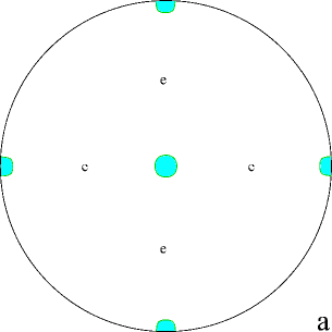
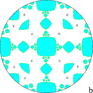
Figure 24: (a) The appearance of the first Stability Zones of the type $(-)$ after passing the value $\,\epsilon^{\cal A}_{1}\,$ by the Fermi level $\,\epsilon_{F}\,$. (b) An increase in the number of Zones of type $(-)$ and the appearance of points of concentration of small Zones at $\,\epsilon_{F}\rightarrow\epsilon^{\cal B}_{1}\,$. (c) Formation of the hole Hall conductivity regions and Zones of types $(\pm)$ and $(+)$ and the appearance of “chaotic” directions of $\,{\bf B}\,$ after passing the value $\,\epsilon^{\cal B}_{1}\,$ by the Fermi level $\,\epsilon_{F}\,$. (d) The disappearance of the electron Hall conductivity regions and Zones of the types $(-)$ and $(\pm)$ at $\,\epsilon_{F}\rightarrow\epsilon^{\cal B}_{2}\,$. (e) The disappearance of the points of concentration of small Zones and the decrease in the number and size of Zones of type $(+)$ after passing the value $\,\epsilon^{\cal B}_{2}\,$ by the Fermi level $\,\epsilon_{F}\,$. (f) Disappearance of the Zones of type $(+)$ in the limit $\,\epsilon_{F}\rightarrow\epsilon^{\cal A}_{2}\,$.

As we noted above, a generic angular diagram of type B contains an infinite number of Stability Zones with arbitrarily large values of topological numbers $\,(M^{1}_{\alpha},M^{2}_{\alpha},M^{3}_{\alpha})$. As it is not difficult to show, a generic angular diagram of type A, on the contrary, contains only a finite number of Zones $\,\Omega_{\alpha}\,$. More precisely, one can see that if $\,\epsilon_{F}\,\in\,(\epsilon^{\cal A}_{1},\epsilon^{\cal B}_{1})\,$ or $\,\epsilon_{F}\,\in\,(\epsilon^{\cal B}_{2},\epsilon^{\cal A}_{2})\,$, then the corresponding angular diagram of the conductivity of the metal contains only a finite number of Stability Zones. Indeed, the presence of an infinite number of Stability Zones means the presence of a point of accumulation of such Zones on $\,\mathbb{S}^{2}\,$, in which we must have the relation $\,{\tilde{\epsilon}}_{1}({\bf B}/B)\,=\,{\tilde{\epsilon}}_{2}({\bf B}/B)\,$, which is impossible in the indicated energy intervals.

It can be seen, therefore, that an angular diagram of type A can contain an infinite number of Stability Zones only in the case $\,\epsilon_{F}\,=\,\epsilon^{\cal B}_{1}\,$ or $\,\epsilon_{F}\,=\,\epsilon^{\cal B}_{2}\,$. It can be also seen that, for the same reason, an angular diagram of conductivity cannot contain “chaotic” directions of $\,{\bf B}\,$ at $\,\epsilon_{F}\,<\,\epsilon^{\cal B}_{1}\,$ or $\,\epsilon_{F}\,>\,\epsilon^{\cal B}_{2}\,$. Recall also that we are considering here angular diagrams of a complex type, i.e. diagrams containing more than one Stability Zone when $\,\epsilon_{F}\,$ changes in the interval $\,(\epsilon^{\cal A}_{1},\epsilon^{\cal A}_{2})\,$.

As can be also seen, both types of complex diagrams (A and B) represent generic diagrams and should be observed experimentally. It should be noted, however, that the diagrams of type B should probably be rather rare due to a small size of the segment $\,(\epsilon^{\cal B}_{1},\epsilon^{\cal B}_{2})\,$ for real dispersion relations. It can also be noted that, although for dispersion laws with close values of $\,\epsilon^{\cal B}_{1}\,$ and $\,\epsilon^{\cal B}_{2}\,$ the probability of observing a type B diagram is rather small, the corresponding diagrams most closely approach the diagrams corresponding to the full dispersion relation in level of complexity.

For the most complete description of all types of angular diagrams arising in the theory of normal metals, it is natural to introduce also the values

$$\epsilon^{{\cal A}\prime}_{1}\,\,\,=\,\,\,\inf\,\,\epsilon_{1}({\bf B}/B)\,\,\,,\quad\epsilon^{{\cal A}\prime}_{2}\,\,\,=\,\,\,\sup\,\,\epsilon_{2}({\bf B}/B)$$

Note, that here we do not concentrate just on the “complicated” Fermi surfaces and include all their types in the consideration.

For values of $\,\epsilon_{F}\,$, lying in the intervals $\,(\epsilon^{{\cal A}\prime}_{1},\epsilon^{\cal A}_{1}]\,$ and $\,[\epsilon^{\cal A}_{2},\epsilon^{{\cal A}\prime}_{2})\,$, the angular diagram of conductivity does not contain finite Stability Zones and can only contain Zones that degenerate into points at $\,\epsilon_{F}=\epsilon^{\cal A}_{1}\,$ or $\,\epsilon_{F}=\epsilon^{\cal A}_{2}\,$. For values of $\,\epsilon_{F}\,$, lying in the intervals $\,(\epsilon^{{\cal A}\prime}_{1},\epsilon^{\cal A}_{1})\,$ and $\,(\epsilon^{\cal A}_{2},\epsilon^{{\cal A}\prime}_{2})\,$, only (unstable) periodic trajectories of the system (I.2) appear on the Fermi surface for special directions of $\,{\bf B}\,$. The corresponding directions of $\,{\bf B}\,$ are represented here by segments of big circles, each of which corresponds to a certain rational direction of open trajectories of the system (I.2). It is not difficult to see also that in the intervals $\,(\epsilon^{{\cal A}\prime}_{1},\epsilon^{\cal A}_{1})\,$ and $\,(\epsilon^{\cal A}_{2},\epsilon^{{\cal A}\prime}_{2})\,$ the number of these segments and the corresponding rational directions of the trajectories is always finite. Indeed, an infinite set of segments of the indicated type must necessarily contain accumulation points on $\,\mathbb{S}^{2}\,$, in each neighborhood of which there are periodic trajectories with arbitrarily large denominators of the corresponding rational directions. For the corresponding directions of $\,{\bf B}\,$ we have the relations $\,\epsilon_{1}({\bf B}/B)\,<\,\tilde{\epsilon}_{1}({\bf B}/B)\,$ (or $\,\epsilon_{2}({\bf B}/B)\,>\,\tilde{\epsilon}_{2}({\bf B}/B)\,$), however, the values $\,|\epsilon_{1}({\bf B}/B)-\tilde{\epsilon}_{1}({\bf B}/B)|\,$ (or $\,|\epsilon_{2}({\bf B}/B)-\tilde{\epsilon}_{2}({\bf B}/B)|\,$) rapidly decrease with increasing denominators of rational directions of periodic trajectories. As a consequence of this, at the corresponding accumulation points we must have the relations $\,\epsilon_{1}({\bf B}/B)\,=\,\tilde{\epsilon}_{1}({\bf B}/B)\,$ or $\,\epsilon_{2}({\bf B}/B)\,=\,\tilde{\epsilon}_{2}({\bf B}/B)\,$, which is impossible in the specified energy intervals. One can also see that when $\,\epsilon_{F}=\epsilon^{\cal A}_{1}\,$ or $\,\epsilon_{F}=\epsilon^{\cal A}_{2}\,$ the set of the directions of $\,{\bf B}\,$, corresponding to the appearance of periodic trajectories on the Fermi surface, may contain an infinite number of segments of big circles corresponding to an infinite number of rational directions of unstable open trajectories.

Finally, in the intervals $\,[\epsilon_{min},\epsilon^{{\cal A}\prime}_{1}]\,$ and $\,[\epsilon^{{\cal A}\prime}_{2},\epsilon_{max}]\,$ system (I.2) cannot contain non-singular open trajectories.

As a result of our reasoning, we can suggest the division of all angular diagrams into “complexity classes” according to the position of the Fermi level with respect to the set of “reference” points defined for a given (generic) dispersion relation. Namely:

(T1) The most simple diagrams:

$$\,\epsilon_{F}\,\,\,\in\,\,\,[\epsilon_{min},\epsilon^{{\cal A}\prime}_{1}]\,$$

The Fermi surface can contain only closed or singular trajectories of the system (I.2) at any direction of $\,{\bf B}\,$. The contribution to the Hall conductivity from the corresponding dispersion relation has the electron type and a constant value (for a given value of $\,B\,$, $\,\omega_{B}\tau\gg 1$) at all directions of $\,{\bf B}\,$.

(T2) Simple enough diagrams:

$$\,\epsilon_{F}\,\,\,\in\,\,\,(\epsilon^{{\cal A}\prime}_{1},\epsilon^{\cal A}_{1}]\,$$

The Fermi surface can contain only closed, singular or unstable periodic open trajectories of the system (I.2). The set of directions of $\,{\bf B}\,$ corresponding to the appearance of periodic open trajectories is represented by a set of segments of big circles, each of which corresponds to a certain rational direction of periodic trajectories. For $\,\epsilon_{F}\,\in\,(\epsilon^{{\cal A}\prime}_{1},\epsilon^{\cal A}_{1})\,$ the set of such segments is finite. For $\,\epsilon_{F}=\epsilon^{\cal A}_{1}\,$ the number of segments and the corresponding rational directions of periodic open trajectories can be infinite. For generic directions of $\,{\bf B}\,$ the contribution to the Hall conductivity of the corresponding dispersion relation has the electron type and a constant value for a given value of $\,B\,$ ($\,\omega_{B}\tau\gg 1$).

(T3) Complex type A diagrams:

$$\,\epsilon_{F}\,\,\,\in\,\,\,(\epsilon^{\cal A}_{1},\epsilon^{\cal B}_{1}]\,$$

In addition to closed and singular trajectories, a generic Fermi surface contains stable open trajectories and unstable periodic trajectories for certain directions of $\,{\bf B}\,$. Stable open trajectories possess the regularity properties described above and arise in special Stability Zones $\,\Omega_{\alpha}\,$ on the angular diagram, corresponding to certain values of topological quantum numbers $\,(M^{1}_{\alpha},M^{2}_{\alpha},M^{3}_{\alpha})\,$. For $\,\epsilon_{F}\,\in\,(\epsilon^{\cal A}_{1},\epsilon^{\cal B}_{1})\,$ the number of Stability Zones at the angular diagram is finite. The set of directions of $\,{\bf B}\,$ corresponding to the appearance of periodic open trajectories is represented by an infinite set of segments of big circles, each of which corresponds to a certain rational direction of periodic trajectories. For $\,\epsilon_{F}=\epsilon^{\cal B}_{1}\,$ the set of Stability Zones $\,\Omega_{\alpha}\,$ becomes infinite in generic case (i.e., for a generic dispersion law); moreover, special directions of $\,{\bf B}\,$, corresponding to the appearance of chaotic open trajectories on the Fermi surface, arise on the angular diagram. For generic directions of $\,{\bf B}\,$ outside the Zones $\,\Omega_{\alpha}\,$ the contribution to the Hall conductivity from the corresponding dispersion relation has the electron type and a constant value for a given value of $\,B\,$ ($\,\omega_{B}\tau\gg 1$).

(T4) Complex type B diagrams:

$$\,\epsilon_{F}\,\,\,\in\,\,\,(\epsilon^{\cal B}_{1},\epsilon^{\cal B}_{2})\,$$

In addition to closed and singular trajectories, a generic Fermi surface contains stable open trajectories, unstable periodic trajectories, and chaotic trajectories for certain directions of $\,{\bf B}\,$. The set of Stability Zones $\,\Omega_{\alpha}\,$, the set of additional segments of big circles, corresponding to the appearance of periodic open trajectories, and the set of special directions of $\,{\bf B}\,$, corresponding to the appearance of chaotic open trajectories on the Fermi surface, are in generic case infinite. For generic directions of $\,{\bf B}\,$ outside the Zones $\,\Omega_{\alpha}\,$ the contribution to the Hall conductivity from the corresponding dispersion relation has different (electron and hole) types in different areas of the angular diagram, separated in generic case by infinite “chains” of Stability Zones and “chaotic” directions of $\,{\bf B}\,$ ($\,\omega_{B}\tau\gg 1$).

(T5) Complex type A diagrams:

$$\,\epsilon_{F}\,\,\,\in\,\,\,[\epsilon^{\cal B}_{2},\epsilon^{\cal A}_{2})\,$$

In addition to closed and singular trajectories, a generic Fermi surface contains stable open trajectories and unstable periodic trajectories for certain directions of $\,{\bf B}\,$. For $\,\epsilon_{F}\,\in\,(\epsilon^{\cal B}_{2},\epsilon^{\cal A}_{2})\,$ the number of Stability Zones at the angular diagram is finite. The set of directions of $\,{\bf B}\,$ corresponding to the appearance of periodic open trajectories is represented by an infinite set of segments of big circles, each of which corresponds to a certain rational direction of periodic trajectories. For $\,\epsilon_{F}=\epsilon^{\cal B}_{2}\,$ the set of Stability Zones $\,\Omega_{\alpha}\,$ is infinite in generic case, besides that, special directions of $\,{\bf B}\,$, corresponding to the appearance of chaotic open trajectories on the Fermi surface, present on the angular diagram. For generic directions of $\,{\bf B}\,$ outside the Zones $\,\Omega_{\alpha}\,$ the contribution to the Hall conductivity from the corresponding dispersion relation has the hole type and a constant value for a given value of $\,B\,$ ($\,\omega_{B}\tau\gg 1$).

(T6) Simple enough diagrams:

$$\,\epsilon_{F}\,\,\,\in\,\,\,[\epsilon^{\cal A}_{2},\epsilon^{{\cal A}\prime}_{2})\,$$

The Fermi surface can contain only closed, singular or unstable periodic open trajectories of the system (I.2). The set of directions of $\,{\bf B}\,$, corresponding to the appearance of periodic open trajectories, is represented by a set of segments of big circles, each of which corresponds to a certain rational direction of periodic trajectories. For $\,\epsilon_{F}\,\in\,(\epsilon^{\cal A}_{2},\epsilon^{{\cal A}\prime}_{2})\,$ the set of such segments is finite. For $\,\epsilon_{F}=\epsilon^{\cal A}_{2}\,$ the number of segments and the corresponding rational directions of periodic open trajectories can be infinite. For generic directions of $\,{\bf B}\,$ the contribution to the Hall conductivity of the corresponding dispersion relation has the hole type and a constant value for a given value of $\,B\,$ ($\,\omega_{B}\tau\gg 1$).

(T7) The most simple diagrams:

$$\,\epsilon_{F}\,\,\,\in\,\,\,[\epsilon^{{\cal A}\prime}_{2},\epsilon_{max}]\,$$

The Fermi surface can contain only closed or singular trajectories of the system (I.2) at any direction of $\,{\bf B}\,$. The contribution to the Hall conductivity from the corresponding dispersion relation has the hole type and a constant value (for a given value of $\,B\,$, $\,\omega_{B}\tau\gg 1$) for all directions of $\,{\bf B}\,$.

Thus, all angular diagrams of conductivity in metals in strong magnetic fields can be assigned to one of the above classes (T1) - (T7), determined by the position of the Fermi level and the dispersion law $\,\epsilon({\bf p})\,$. Note again that the full picture of the angle diagrams for all values of $\,\epsilon_{F}\,$ is somewhat abstract in nature, since only the diagram for the real value of $\,\epsilon_{F}\,$ is experimentally observable. In particular, in experimental change of the position of $\,\epsilon_{F}\,$ (for example, using external pressure) the change in the corresponding conductivity diagram is not required to be determined by the initial relation $\,\epsilon({\bf p})\,$, since the corresponding external influence changes also the parameters of the dispersion relation. The above remark, however, does not cancel the fact that the type of a specific angular diagram is determined unambiguously on the basis of the theoretical consideration given above. Let us note again that our considerations here can be considered as quite general for arbitrary “physically realistic” dispersion relation $\,\epsilon({\bf p})\,$. At the same time, we omit here some theoretically possible additional features (f.e. non-simply-connectedness of Stability Zones) which are extremely unlikely in a real situation.

Another remark that can be made here relates to the fact that, in the general case, the full Fermi surface represents the union of several components related to different dispersion relations. It is easy to see that the angular diagram of conductivity is given in this case by the “overlapping” of the diagrams defined by all the components. An important circumstance here is that if different components do not intersect with each other, then the intersection of the corresponding Stability Zones is possible only if these Zones correspond to the same topological numbers $\,(M^{1}_{\alpha},M^{2}_{\alpha},M^{3}_{\alpha})\,$. As a consequence, such intersecting Zones can be viewed as complex “composite” Zones with a more complex border structure.

Here, of course, we should also say a few words about angular diagrams (for fixed values of $\,\epsilon_{F}$) arising for dispersion relations with only one Stability Zone $\,\Omega\,$ (occupying the entire sphere $\,\mathbb{S}^{2}$). It must be said that the dispersion relations of this type also represent generic relations and may well occur in real crystals. (In particular, such relations include relations for which in a certain energy interval the surfaces $\,\epsilon({\bf p})\,=\,const\,$ represent a set of periodically deformed (“corrugated”) integral planes that are not connected to each other.) We omit here a detailed analysis of the situation arising in this case and give only a general description of the complexity classes of angular diagrams arising here for different values of $\,\epsilon_{F}\,$.

Namely, as in the case of dispersion relations with “complex” angular diagrams, in the situation we are considering it is also possible in generic case to introduce some “reference” values

$$\epsilon_{\min}\,<\,\hat{\epsilon}^{{\cal A}\prime}_{1}\,<\,\hat{\epsilon}^{\cal A}_{1}\,<\,\hat{\epsilon}^{\cal B}_{1}\,<\,\hat{\epsilon}^{\cal B}_{2}\,<\,\hat{\epsilon}^{\cal A}_{2}\,<\,\hat{\epsilon}^{{\cal A}\prime}_{2}\,<\,\epsilon_{\max}$$

and classes of diagrams (T1) - (T7), similar to those considered above. Here the classes (T1), (T2), (T6), (T7) completely coincide with the corresponding classes described above, and for the diagrams of the classes (T3) and (T5), only the words “the number of Stability Zones at the angular diagram is finite” need to be replaced to “we have one Stability Zone $\,\Omega\,$, occupying part of the sphere $\,\mathbb{S}^{2}\,$” . (We do not require here the connectedness of the Zone $\,\Omega\,$ and, in particular, we consider as the same Zone possibly separated opposite parts on $\,\mathbb{S}^{2}$.) As for the class (T4), the diagrams of this class contain here just one Stability Zone $\,\Omega\,$, which occupies the whole sphere $\,\mathbb{S}^{2}\,$. Note here, that for the class (T4) theoretically we could also have a Stability Zone $\,\Omega\,$, occupying a part of $\,\mathbb{S}^{2}\,$, with different signs of the Hall conductivity in different regions outside $\,\Omega\,$. This situation, however, corresponds to non-simply-connected Zone $\,\Omega\,$ and physically is extremely unlikely, so, we do not bring it here.

Note also that the above mentioned “reference” energy values are quite simply related to the “reference” values defined for dispersion relations, which have “complex” angular diagrams. Thus, we can actually write the relations

$$\hat{\epsilon}^{{\cal A}\prime}_{1}\,=\,\epsilon^{{\cal A}\prime}_{1}\,\,,\quad\hat{\epsilon}^{\cal A}_{1}\,=\,\epsilon^{\cal A}_{1}\,\,,\quad\hat{\epsilon}^{\cal A}_{2}\,=\,\epsilon^{\cal A}_{2}\,\,,\quad\hat{\epsilon}^{{\cal A}\prime}_{2}\,=\,\epsilon^{{\cal A}\prime}_{2}$$

according to the definition of the values $\,\epsilon^{{\cal A}\prime}_{1}\,$, $\,\epsilon^{\cal A}_{1}\,$, $\,\epsilon^{\cal A}_{2}\,$, $\,\epsilon^{{\cal A}\prime}_{2}\,$, given above.

As for the values $\,\hat{\epsilon}^{\cal B}_{1}\,$ and $\,\hat{\epsilon}^{\cal B}_{2}\,$, for them we have the relations

$$\hat{\epsilon}^{\cal B}_{1}\,\,\,=\,\,\,\epsilon^{\cal B}_{2}\,\,\,=\,\,\,\max\,\,\tilde{\epsilon}_{1}({\bf B}/B)\,\,\,,$$

$$\hat{\epsilon}^{\cal B}_{2}\,\,\,=\,\,\,\epsilon^{\cal B}_{1}\,\,\,=\,\,\,\min\,\,\tilde{\epsilon}_{2}({\bf B}/B)\,\,\,,$$

since for the dispersion laws of the type under consideration we have in our case the relation $\,\epsilon^{\cal B}_{1}\,>\,\epsilon^{\cal B}_{2}\,$. (Note again, that theoretically also the situation $\,\epsilon^{\cal B}_{1}<\epsilon^{\cal B}_{2}\,$ and $\,\hat{\epsilon}^{\cal B}_{1}=\epsilon^{\cal B}_{1}\,$, $\,\,\hat{\epsilon}^{\cal B}_{2}=\epsilon^{\cal B}_{2}\,$ is possible here but is extremely unlikely according to our remarks above).

It is not difficult to see also that in this case no angular diagrams can contain directions of $\,{\bf B}\,$ corresponding to the appearance of “chaotic” trajectories on the Fermi surface.

In conclusion, we make here a comparison of the complexity of the location of the Stability Zones on angular diagrams for fixed Fermi surfaces with the location of the Zones $\,\Omega^{*}_{\alpha}\,$ on the diagrams for the entire dispersion law. More specifically, we will consider here an analogue of the structure of Zones, presented at Fig. 16, for diagrams defined for a fixed value of $\,\epsilon_{F}\,$.

As we have already seen, angular diagrams of conductivity for fixed values of $\,\epsilon_{F}\,$ may, in particular, be quite simple and not have a level of complexity comparable to the level of complexity of angular diagrams for the entire relation $\,\epsilon({\bf p})\,$. We, therefore, will be interested in diagrams (of type A or B) containing the Stability Zones $\,\Omega_{\alpha}\,$, which are close in shape to the corresponding Stability Zones $\,\Omega^{*}_{\alpha}\,$, defined for the entire dispersion relation. As it is not difficult to see, such Zones are Stability Zones, the first and second borders of which are located quite close to each other (Fig. 21, b, c, d). As we have indicated earlier, in the domain $\,\Omega^{\prime}_{\alpha}\,$, bounded by the first and second boundary of the Zone $\,\Omega_{\alpha}\,$, there can not appear stable open trajectories of system (I.2), and, correspondingly, there can be no other Stability Zones for a given value of $\,\epsilon_{F}\,$. It can be seen, therefore, that structures similar to those shown at Fig. 16, if they arise, must be connected in this case with the second boundary of the Zone $\,\Omega_{\alpha}\,$.

To describe the picture that appears in our case, it is necessary to turn again to the structure of the Fermi surface at $\,{\bf B}/B\,\in\,\Omega_{\alpha}\,$ (Fig. 10), as well as to the mechanism of destruction of this structure on the first and second boundaries of $\,\Omega_{\alpha}\,$ by the “jumps” of trajectories from one carrier of open trajectories to another represented at Fig. 11. To simplify the description, it is convenient to consider the projection of the ‘carriers of open trajectories’ on the plane $\,\Pi({\bf B}/B)\,$ generated by the direction of $\,{\bf B}\,$, and also the direction of intersection of the plane orthogonal to $\,{\bf B}\,$ and the plane $\,\Gamma_{\alpha}\,$. All trajectories of system (I.2) will be represented in this plane by parallel straight lines orthogonal to $\,{\bf B}\,$. After crossing the first boundary of $\,\Omega_{\alpha}\,$ and arising of trajectories jumps from one carrier to another (Fig. 11), for each carrier on the projection we can mark “places”, where trajectories jump between pairs of “merged” carriers. In this case, both former carriers from each resulting pair can be represented by the same projection on the plane $\,\Pi({\bf B}/B)\,$, and the “places” where the jumps occur can be denoted by circles of a small radius (although it is not very precise). It can be said that such circles represent “traps”, falling into which a trajectory jumps from one former carrier of open trajectories (for a fixed pair) to another and back.

Each of the carriers of open trajectories represents a periodically deformed integral plane in $\,{\bf p}$ - space and, thus, a picture arising in the plane $\,\Pi({\bf B}/B)\,$ is always doubly periodic. (Note also that the holes (flat disks) in the carriers of open trajectories disappear on the projection, being orthogonal to $\,{\bf B}$). In particular, the arrangement of the “traps” described by us for each pair of “merged” carriers of open trajectories is doubly periodic.

Straight lines that represent the trajectories of the system (I.2) after crossing the boundary of $\,\Omega_{\alpha}\,$ become in general “cut” into segments of finite length. It is not difficult to see that each of these segments, bounded by “traps” at both its ends, represents a (long) closed trajectory of the system (I.2) arising on a pair of former carriers of open trajectories after crossing the boundary of a Stability Zone. It can also be seen that if the intersection of a plane, orthogonal to $\,{\bf B}\,$, and $\,\Gamma_{\alpha}\,$ has an irrational direction, then all former open trajectories turn into closed ones after crossing the boundary of $\,\Omega_{\alpha}\,$ (Fig. 25, a). At the same time, if the mean direction of open trajectories is rational, then immediately after crossing the first boundary of $\,\Omega_{\alpha}\,$ on a pair of former carriers of open trajectories both long closed trajectories and “intact” periodic open trajectories will be present (Fig. 25, b).

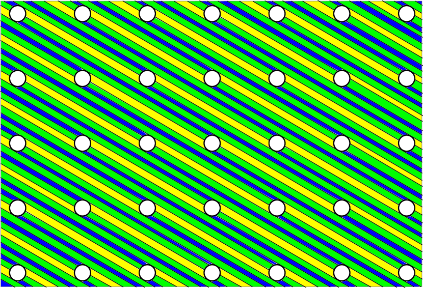
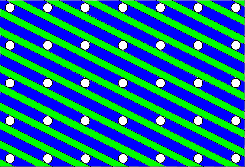
Figure 25: (a) Projections of long closed trajectories of system (I.2) arising after crossing the boundary of a Stability Zone for an irrational mean direction of open trajectories. (b) Projections of long closed and open periodic trajectories of system (I.2) present after crossing the boundary of a Stability Zone for a rational mean direction of open trajectories.

The diameters of the “traps” tend to zero when approaching the boundary of the Zone $\,\Omega_{\alpha}\,$ from the outside and increase when moving away from it (near $\,\Omega_{\alpha}$). It can be seen here that for each rational direction of open trajectories there actually exists a critical radius of “traps”, for which the layers of open trajectories disappear due to their complete overlap by “traps”. In addition, it can also be seen that the critical radius of “traps” decreases rather quickly with increasing of “denominators” of the corresponding rational directions of the trajectories. As a consequence, the segments adjacent to the boundary of a Stability Zone and corresponding to the appearance of unstable periodic trajectories on the Fermi surface (Fig. 17) form an everywhere dense set on the boundary of $\,\Omega_{\alpha}\,$, however, at any finite distance from the boundary the number of such segments is finite. For our consideration here, the segments that reach the second boundary of a Stability Zone will be important.

As was noted above, in each connected component of the domain $\,\Omega^{\prime}_{\alpha}\,$, adjacent to a certain part of the first boundary of the Zone $\,\Omega_{\alpha}\,$, for all generic directions of $\,{\bf B}\,$ the same type of the Hall conductivity appear, which is opposite to the type of the cylinder of closed trajectories vanishing at the corresponding part of the first boundary of $\,\Omega_{\alpha}\,$. At the corresponding section of the second boundary of $\,\Omega_{\alpha}\,$ the cylinder of closed trajectories of the opposite type (relative to the type of the cylinder disappearing at the first boundary) disappears and trajectories start to jump between pairs of “merged” former carriers of open trajectories (Fig. 10). Thus, on the above projection of the former carriers of open trajectories on the plane $\,\Pi({\bf B}/B)\,$ “traps of the second type” appear, getting into which a trajectory jumps between pairs of “merged” carriers. Like the “traps of the first type”, the “traps of the second type” form a periodic structure in the plane $\,\Pi({\bf B}/B)\,$ (Fig. 26).

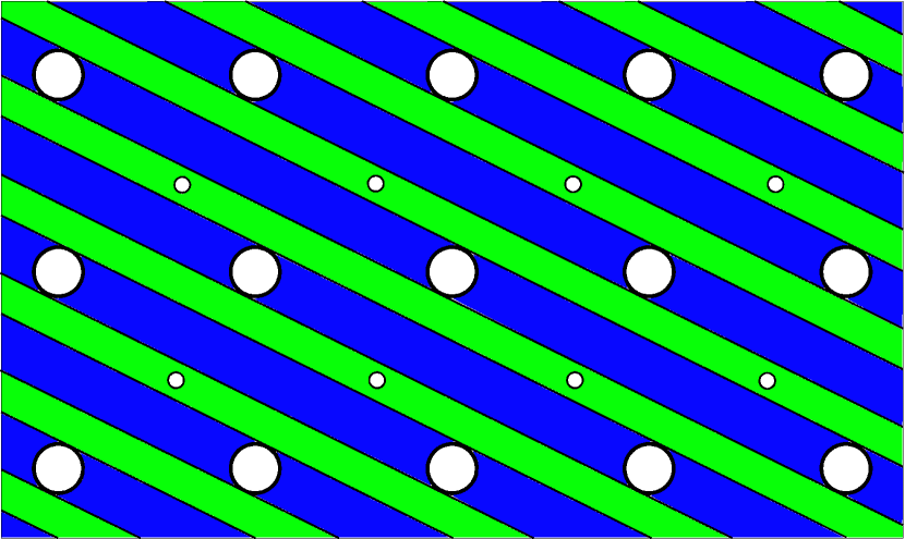
Figure 26: Traps of the second type, arising after crossing the second boundary of the Zone $\,\Omega_{\alpha}\,$.

At Fig. 26 we have actually represented the projections of only half of the “traps of the second type” arising on a pair of “merged” carriers of open trajectories, namely, the “traps” lying on the “upper” carrier and corresponding to jumping to one of the neighboring pairs of similar carriers. The projection of the neighboring pair of “merged” carriers onto the plane $\,\Pi({\bf B}/B)\,$ coincides with the projection of the pair under consideration shifted by some vector in this plane. It can be said, therefore, that each of the “traps of the second type” actually has an upper and a lower base, lying in different parts of the picture, represented at Fig. 25a or Fig. 25b.

The diameters of the “traps of the second type” tend to zero when approaching the second boundary of the Zone $\,\Omega_{\alpha}\,$ from the outside and increase when moving away from it (near $\,\Omega_{\alpha}$). After crossing the second boundary of $\,\Omega_{\alpha}\,$ “traps of the second type” arise in the form of points at Fig. 25a or Fig. 25b, having “upper and lower bases” on cylinders of closed trajectories or on layers of periodic trajectories (if any) of the system (I.2).

Here we will consider only “physical” dispersion laws that satisfy the requirement $\,\epsilon({\bf p})\,=\,\epsilon(-{\bf p})\,$, which also implies invariance of the Fermi surface under the transformation $\,{\bf p}\,\rightarrow\,-{\bf p}\,$. It is not difficult to check then, that the invariance of the structure of the system (I.2) with respect to the same transformation also implies in our situation the symmetry of the upper and lower bases of the “traps of the second type”. In particular, each newly appeared after crossing the second boundary of the Zone $\,\Omega_{\alpha}\,$ (small) “trap of the second type” interconnects (in the generic case) either long closed trajectories of the system (I.2) or periodic open trajectories. As can be seen, these two cases correspond to substantially different structures of trajectories of system (I.2) on the Fermi surface after crossing the second boundary of the Zone $\,\Omega_{\alpha}\,$.

Indeed, as is not difficult to see, the reconstruction of the second type corresponds to the picture presented at Fig. 27. It can also be seen that, both before the restructuring and after the restructuring of the trajectories, the Fermi surface contains only closed trajectories of the system (I.2) and pictures in all planes orthogonal to $\,{\bf B}\,$ have the same type (I or II) in both cases. Thus, after the reconstruction of the trajectories described above, the corresponding directions of $\,{\bf B}\,$ lie outside any of the Stability Zones $\,\Omega_{\beta}\,$ and the total contribution of the Fermi surface to the Hall conductivity does not change. This situation takes place, in particular, when crossing the second boundary of the Zone $\,\Omega_{\alpha}\,$ at generic points, as well as at points corresponding to rational directions of intersection of $\,\Gamma_{\alpha}\,$ and the plane orthogonal to $\,{\bf B}\,$ if the diameter of the “traps of the first type” exceeds the critical one (the corresponding “additional segments” do not reach the second boundary).

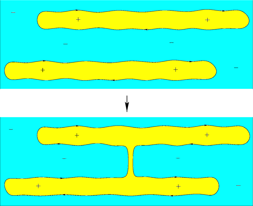
Figure 27: The reconstruction of trajectories of system (I.2) after crossing of the second boundary of $\,\Omega_{\alpha}\,$ in the case when the “traps of the second type” appear on the cylinders of closed trajectories.

In another case, when the “traps of the second type” appear on the layers of periodic open trajectories of the system (I.2), the corresponding reconstruction of the trajectories can be represented by the picture shown at Fig. 28. In this case both pictures (I and II) appear in the planes orthogonal to $\,{\bf B}\,$ being separated by open trajectories of the system (I.2) (Fig. 29). Such a situation can occur only when the second boundary of a Stability Zone is crossed at a point corresponding to the presence of periodic open trajectories of (I.2) on the Fermi surface, i.e. at a point of intersection of the second boundary with an additional segment adjacent to the boundary of the Stability Zone and corresponding to the appearance of unstable periodic trajectories on the Fermi surface. We note at the same time, that even in this case the situation can also be described by the picture presented at Fig. 27 if the “traps of the second type” appear on cylinders of closed trajectories.

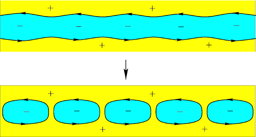
Figure 28: The reconstruction of trajectories of system (I.2) after crossing of the second boundary of $\,\Omega_{\alpha}\,$ in the case when the “traps of the second type” appear on layers of periodic open trajectories.

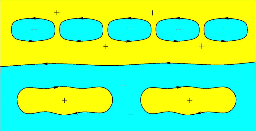
Figure 29: Situations I and II in a plane orthogonal to $\,{\bf B}\,$, separated by open trajectories of (I.2).

The closed trajectories shown at Fig. 29 cut the Fermi surface into new carriers of open trajectories, corresponding to the appearance of a new Stability Zone $\,\Omega_{\beta}\,$. The Zone $\,\Omega_{\beta}\,$, defined for a fixed Fermi surface, belongs to one of the Zones $\,\Omega^{*}_{\beta}\,$ shown at Fig. 16.

The picture presented at Fig. 29 is locally stable (with respect to small rotations of the direction of $\,{\bf B}$) and is preserved until a reconstruction of the closed trajectories shown on it occurs. It can be seen that near the second boundary of the Zone $\,\Omega_{\alpha}\,$ the region of stability of the picture shown at Fig. 29 is determined by the diameter of the “traps of the second type”, which in this situation is small compared to the diameter of the “traps of the first type”. Thus, the allowable angle of deviation of the direction of intersection of the plane $\,\Gamma_{\alpha}\,$ with the plane orthogonal to $\,{\bf B}\,$ for a fixed small diameter of the “traps of the second type” is proportional to this diameter, which determines the allowable angle of deviation of the direction of $\,{\bf B}\,$ in parallel to the second boundary (Fig. 30). Since the diameter of the “traps of the second type” is proportional to the distance to the second boundary of the Zone $\,\Omega_{\alpha}\,$, it can be seen also that the boundary of the Zone $\,\Omega_{\beta}\,$ must have a “corner” on the second boundary of $\,\Omega_{\alpha}\,$ (Fig. 31).

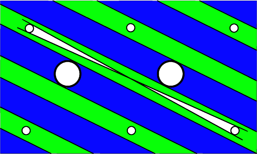
Figure 30: The allowable angle of deviation of the intersection of $\,\Gamma_{\alpha}\,$ with the plane orthogonal to $\,{\bf B}\,$ for a fixed diameter of the “traps of the second type”.

Figure 31: The Stability Zones $\,\Omega_{\beta}\,$ adjacent to the second boundary of the Zone $\,\Omega_{\alpha}\,$ in part of its “rational” points.

As we have already said above, the appearance of a new Stability Zone on the second boundary of the Zone $\,\Omega_{\alpha}\,$ may not occur even at the intersection points of the second boundary with “additional segments” adjacent to $\,\Omega_{\alpha}\,$ and representing the directions of $\,{\bf B}\,$ corresponding to the appearance of unstable periodic trajectories on the Fermi surface. This situation occurs if, despite the presence of layers of periodic trajectories on the Fermi surface, the appearance of the “traps of the second type” occurs on cylinders of closed trajectories of the system (I.2). Thus, in the general case, the boundary of $\,\Omega_{\alpha}\,$ can be divided into segments in which new Zones are born at the described intersection points, and into segments in which new Zones are not born (Fig. 32). It can be noted that, since the height of the cylinders of closed trajectories is determined in this case by the diameter of the “traps of the first type”, the general measure of the segments of the second type will be the smaller, the closer the second boundary of the Zone $\,\Omega_{\alpha}\,$ is to its first boundary. In addition, one can also notice that for segments of the second type, the appearance of new Zones $\,\Omega_{\beta}\,$ on the segments of special directions of $\,{\bf B}\,$ theoretically can occur at some distance from the second boundary of $\,\Omega_{\alpha}\,$ as a result of mutual displacement of “traps” of the first and second types.

In general, it can be noted that the structure of the angular diagrams for a fixed Fermi surface can be quite close to the structure of the diagrams for the entire dispersion law near the special Stability Zones discussed above.

Figure 32: Segments of the boundary of a Zone $\,\Omega_{\alpha}\,$ corresponding to the appearance and absence of new Stability Zones at the points of intersection of the second boundary with segments of special directions of $\,{\bf B}\,$.

V Conclusion

We considered angular diagrams for conductivity in metals with arbitrary (physical) Fermi surfaces. As it turns out, it is natural to divide all angular diagrams into a finite number of “complexity classes” that have a quite effective geometric description. The most interesting, from our point of view, are the most complex diagrams (of type B), containing an infinite number of Stability Zones, as well as directions of $\,{\bf B}\,$, corresponding to the appearance of “chaotic” trajectories on the Fermi surface. The paper also provides some comparison of the complexity of such diagrams with diagrams defined for the entire dispersion law.

The study was carried out at the expense of a grant from the Russian Science Foundation (project №  18-11-00316).

References

- (1) C. Kittel., Quantum Theory of Solids., Wiley, 1963.
- (2) J.M. Ziman., Principles of the Theory of Solids., Cambridge University Press 1972.
- (3) A.A. Abrikosov., Fundamentals of the Theory of Metals., Elsevier Science & Technology, Oxford, United Kingdom, 1988.
- (4) I.M.Lifshitz, M.Ya.Azbel, M.I.Kaganov. The Theory of Galvanomagnetic Effects in Metals., Sov. Phys. JETP 4:1, 41-53 (1957).
- (5) I.M. Lifshitz, V.G. Peschansky., Galvanomagnetic characteristics of metals with open Fermi surfaces., Sov. Phys. JETP 8:5, 875-883 (1959).
- (6) I.M. Lifshitz, V.G. Peschansky., Galvanomagnetic characteristics of metals with open Fermi surfaces. II., Sov. Phys. JETP 11:1, 131-141 (1960).
- (7) I.M. Lifshitz, M.I. Kaganov., Some problems of the electron theory of metals I. Classical and quantum mechanics of electrons in metals., Sov. Phys. Usp. 2:6 (1960), 831-835.
- (8) I.M. Lifshitz, M.I. Kaganov., Some problems of the electron theory of metals II. Statistical mechanics and thermodynamics of electrons in metals., Sov. Phys. Usp. 5:6 (1963), 878-907.
- (9) I.M. Lifshitz, M.I. Kaganov., Some problems of the electron theory of metals III. Kinetic properties of electrons in metals., Sov. Phys. Usp. 8:6 (1966), 805-851.
- (10) I.M. Lifshitz, M.Ya. Azbel, M.I. Kaganov., Electron Theory of Metals. Moscow, Nauka, 1971. Translated: New York: Consultants Bureau, 1973.
- (11) Conductivity electrons., Red. M.I. Kaganov, V.S. Edelman., Moscow, Nauka, 1985 (in Russian).
- (12) M.I. Kaganov, V.G. Peschansky., Galvano-magnetic phenomena today and forty years ago., Physics Reports 372 (2002), 445-487.
- (13) S.P. Novikov., The Hamiltonian formalism and a many-valued analogue of Morse theory., Russian Math. Surveys 37 (5) (1982), 1-56.
- (14) A.V. Zorich., A problem of Novikov on the semiclassical motion of an electron in a uniform almost rational magnetic field., Russian Math. Surveys 39 (5) (1984), 287-288.
- (15) I.A. Dynnikov., Proof of S.P. Novikov’s conjecture for the case of small perturbations of rational magnetic fields., Russian Math. Surveys 47 (3) (1992), 172-173.
- (16) I.A. Dynnikov., Proof of S.P. Novikov’s conjecture on the semiclassical motion of an electron., Math. Notes 53:5 (1993), 495-501.
- (17) S.P. Novikov, A.Y. Maltsev., Topological quantum characteristics observed in the investigation of the conductivity in normal metals., JETP Letters 63 (10) (1996), 855-860.
- (18) S.P. Novikov, A.Y. Maltsev., Topological phenomena in normal metals., Physics-Uspekhi 41:3 (1998), 231-239.
- (19) S.P. Tsarev. Private communication. (1992-93).
- (20) I.A. Dynnikov., Semiclassical motion of the electron. A proof of the Novikov conjecture in general position and counterexamples., Solitons, geometry, and topology: on the crossroad, Amer. Math. Soc. Transl. Ser. 2, 179, Amer. Math. Soc., Providence, RI, 1997, 45-73.
- (21) A.Y. Maltsev., Anomalous behavior of the electrical conductivity tensor in strong magnetic fields., JETP 85 (5) (1997), 934-942.
- (22) A.Ya. Maltsev, S.P. Novikov., The theory of closed 1-forms, levels of quasiperiodic functions and transport phenomena in electron systems., Proceedings of the Steklov Institute of Mathematics, 2018, Vol. 302, pp. 279–297, arXiv:1805.05210
- (23) I.A. Dynnikov., The geometry of stability regions in Novikov’s problem on the semiclassical motion of an electron., Russian Math. Surveys 54:1 (1999), 21-59.
- (24) I.A. Dynnikov., Surfaces in 3-torus: geometry of plane sections., Proc. of ECM2, BuDA, 1996.
- (25) I.A. Dynnikov, A.Ya. Maltsev., Topological characteristics of electronic spectra of single crystals., Journal of Experimental and Theoretical Physics 85:1 (1997), 205-208.
- (26) A.Ya. Maltsev, S.P. Novikov., Quasiperiodic functions and Dynamical Systems in Quantum Solid State Physics., Bulletin of Braz. Math. Society, New Series 34:1 (2003), 171-210.
- (27) A.Ya. Maltsev, S.P. Novikov., Dynamical Systems, Topology and Conductivity in Normal Metals in strong magnetic fields., Journal of Statistical Physics 115:(1-2) (2004), 31-46.
- (28) A.Ya. Maltsev, S.P. Novikov., Dynamical Systems, Topology and Conductivity in Normal Metals., arXiv:cond-mat/0304471
- (29) R. De Leo., First-principles generation of stereographic maps for high-field magnetoresistance in normal metals: An application to Au and Ag., Physica B: Condensed Matter 362 (1–4) (2005), 62–75.
- (30) A.Ya. Maltsev., On the Analytical Properties of the Magneto-Conductivity in the Case of Presence of Stable Open Electron Trajectories on a Complex Fermi Surface., Journal of Experimental and Theoretical Physics 124 (5) (2017), 805-831.
- (31) A.Ya. Maltsev., Oscillation phenomena and experimental determination of exact mathematical Stability Zones for magneto-conductivity in metals having complicated Fermi surfaces., Journal of Experimental and Theoretical Physics 125 (5) (2017), 896–905.
- (32) A.Ya. Maltsev., The second boundaries of Stability Zones and the angular diagrams of conductivity for metals having complicated Fermi surfaces., Journal of Experimental and Theoretical Physics 127:6 (2018), 1087-1111., arXiv:1804.10762
- (33) A.V. Zorich., Proc. “Geometric Study of Foliations”., (Tokyo, November 1993) / ed. T.Mizutani et al. Singapore: World Scientific, 479-498 (1994).
- (34) A.V. Zorich., Finite Gauss measure on the space of interval exchange transformations. Lyapunov exponents., Annales de l’Institut Fourier 46:2, (1996), 325-370.
- (35) Anton Zorich., On hyperplane sections of periodic surfaces., Solitons, Geometry, and Topology: On the Crossroad, V. M. Buchstaber and S. P. Novikov (eds.), Translations of the AMS, Ser. 2, vol. 179, AMS, Providence, RI (1997), 173-189.
- (36) Anton Zorich., How do the leaves of closed 1-form wind around a surface., “Pseudoperiodic Topology”, V.I.Arnold, M.Kontsevich, A.Zorich (eds.), Translations of the AMS, Ser. 2, vol. 197, AMS, Providence, RI, 1999, 135-178.
- (37) R. De Leo., Existence and measure of ergodic leaves in Novikov’s problem on the semiclassical motion of an electron., Russian Math. Surveys 55:1 (2000), 166-168.
- (38) R. De Leo., Characterization of the set of “ergodic directions” in Novikov’s problem of quasi-electron orbits in normal metals., Russian Math. Surveys 58:5 (2003), 1042-1043.
- (39) R. De Leo., Topology of plane sections of periodic polyhedra with an application to the Truncated Octahedron., Experimental Mathematics 15:1 (2006), 109-124.
- (40) Anton Zorich., Flat surfaces., in collect. “Frontiers in Number Theory, Physics and Geometry. Vol. 1: On random matrices, zeta functions and dynamical systems”; Ecole de physique des Houches, France, March 9-21 2003, P. Cartier; B. Julia; P. Moussa; P. Vanhove (Editors), Springer-Verlag, Berlin, 2006, 439-586.
- (41) R. De Leo, I.A. Dynnikov., An example of a fractal set of plane directions having chaotic intersections with a fixed 3-periodic surface., Russian Math. Surveys 62:5 (2007), 990–992.
- (42) R. De Leo, I.A. Dynnikov., Geometry of plane sections of the infinite regular skew polyhedron ., Geom. Dedicata 138:1 (2009), 51-67.
- (43) A. Skripchenko., Symmetric interval identification systems of order three., Discrete Contin. Dyn. Sys. 32:2 (2012), 643-656.
- (44) A. Skripchenko., On connectedness of chaotic sections of some 3-periodic surfaces., Ann. Glob. Anal. Geom. 43 (2013), 253-271.
- (45) I. Dynnikov, A. Skripchenko., On typical leaves of a measured foliated 2-complex of thin type., Topology, Geometry, Integrable Systems, and Mathematical Physics: Novikov’s Seminar 2012-2014, Advances in the Mathematical Sciences., Amer. Math. Soc. Transl. Ser. 2, 234, eds. V.M. Buchstaber, B.A. Dubrovin, I.M. Krichever, Amer. Math. Soc., Providence, RI, 2014, 173-200, arXiv: 1309.4884
- (46) I. Dynnikov, A. Skripchenko., Symmetric band complexes of thin type and chaotic sections which are not actually chaotic., Trans. Moscow Math. Soc., Vol. 76, no. 2, 2015, 287-308.
- (47) A. Avila, P. Hubert, A. Skripchenko., Diffusion for chaotic plane sections of 3-periodic surfaces., Inventiones mathematicae, October 2016, Volume 206, Issue 1, pp 109–146.
- (48) A. Avila, P. Hubert, A. Skripchenko., On the Hausdorff dimension of the Rauzy gasket., Bulletin de la societe mathematique de France, 2016, 144 (3), pp. 539 - 568.
- (49) Roberto De Leo., A survey on quasiperiodic topology., arXiv:1711.01716