ABSTRACT

In the literature, it was proposed that the growth index $\gamma$ is useful to distinguish the scenarios of dark energy and modified gravity. In the present work, we consider the constraints on the growth index $\gamma$ by using the latest observational data. To be model-independent, we use cosmography to describe the cosmic expansion history, and also expand the general $\gamma(z)$ as a Taylor series with respect to redshift $z$ or $y$-shift, $y=z/(1+z)$. We find that the present value $\gamma_{0}=\gamma(z=0)\simeq 0.42$ (for most of viable $f(R)$ theories) is inconsistent with the latest observational data at high confidence level (C.L.). On the other hand, $\gamma_{0}\simeq 0.55$ (for dark energy models in GR) can be consistent with the latest observational data at $1\sigma$ C.L. in 5 of the 9 cases under consideration, but is inconsistent beyond $2\sigma$ C.L. in the other 4 cases (while it is still consistent within the $3\sigma$ region). Thus, we can say nothing firmly about $\gamma_{0}\simeq 0.55$. We also find that a varying $\gamma(z)$ is favored.

Observational Constraints on Growth Index
with Cosmography

I Introduction

It is a great mystery since the current accelerated expansion of our universe was discovered in 1998 Riess:1998cb ; Perlmutter:1998np . More than 20 years passed, and we still do not know the very nature of the cosmic acceleration by now. Usually, an unknown energy component with negative pressure (dark energy) is introduced to interpret this mysterious phenomenon in general relativity (GR). Alternatively, one can make a modification to GR (modified gravity). In fact, modified gravity can also successfully explain the cosmic acceleration without invoking dark energy. So far, these two scenarios are both competent Ishak:2018his ; Amendola:2016saw ; Joyce:2014kja ; Clifton:2011jh .

In order to understand the nature of the cosmic accelerated expansion, one of the most important tasks is to distinguish between the scenarios of dark energy and modified gravity. If the observational data could help us to confirm or exclude one of these two scenarios as the real cause of this mysterious phenomenon, it will be a great step forward. However, many cosmological observations merely probe the cosmic expansion history. Unfortunately, as is well known (see e.g. Sahni:2006pa ), one can always build models sharing a same cosmic expansion history, and hence these models cannot be distinguished by using the observational data of the expansion history only. So, some independent and complementary probes are required. Later, it is proposed that if the cosmological models share a same cosmic expansion history, they might have different growth histories, which are characterized by the matter density contrast $\delta(z)\equiv\delta\rho_{m}/\rho_{m}$ as a function of redshift $z$. Therefore, they might be distinguished from each other by combining the observations of both the expansion and growth histories (see e.g. Linder:2005in ; Linder:2007hg ; Huterer:2006mva ; Wang:2007ht ; Zhang:2007nk ; Jain:2007yk ; Wei:2008ig ; Wei:2008vw ; Wei:2013rea ; Yin:2018mvu ; Viznyuk:2018eiz ; Amendola:2014yca ; Basilakos:2016nyg and references therein).

It is convenient to introduce the growth rate $f\equiv d\ln\delta/d\ln a$, where $a=(1+z)^{-1}$ is the scale factor. As is well known, a good parameterization for the growth rate is given by Peebles1980 ; Lahav:1991wc ; Wang:1998gt ; Lue:2004rj

$$f\equiv\frac{d\ln\delta}{d\ln a}=\Omega_{m}^{\gamma}\,,$$ (1)

where $\gamma$ is the growth index, and $\Omega_{m}$ is the fractional energy density of matter. Beginning in e.g. Linder:2005in ; Linder:2007hg , it was advocated that the growth index $\gamma$ is useful to distinguish the scenarios of dark energy and modified gravity. For example, it is found that $\gamma=6/11\simeq 0.545$ for $\Lambda$CDM model Linder:2005in ; Linder:2007hg , and $\gamma\simeq 0.55$ for most of dark energy models in GR Linder:2005in . In fact, they are clearly distinct from the ones of modified gravity theories. For instance, it is found that $\gamma\simeq 0.68$ for Dvali-Gabadadze-Porrati (DGP) braneworld model Linder:2007hg ; Wei:2008ig , and $\gamma\simeq 0.42$ for most of viable $f(R)$ theories Gannouji:2008wt ; Tsujikawa:2009ku ; Shafieloo:2012ms ; Tsujikawa:2010zza . In general, the growth index $\gamma$ is a function of redshift $z$. It is argued that $\gamma(z)$ lies in a relatively narrow range around the above values respectively, and hence one might distinguish between them.

In the literature, most of the relevant works assumed a particular cosmological model to obtain the growth index $\gamma$. Thus, the corresponding results are model-dependent in fact. However, robust results should be model-independent. So, it is of interest to obtain the growth index $\gamma$ from the observational data by using a model-independent approach. In fact, recently we have made an effort in Yin:2018mvu to obtain a non-parametric reconstruction of the growth index $\gamma$ via Gaussian processes by using the latest observational data. Although the approach of Gaussian processes is clearly model-independent, its reliability at high redshift might be questionable. So, it is of interest to test the growth index $\gamma$ by using a different method, and cross-check the corresponding results with the ones from Gaussian processes.

As is well known, one of the powerful model-independent approaches is cosmography Weinberg1972 ; Visser:2003vq ; Bamba:2012cp ; Cattoen:2008th ; Vitagliano:2009et ; Cattoen:2007id ; Xu:2010hq ; Xia:2011iv ; Zhang:2016urt ; Dunsby:2015ers ; Luongoworks ; Zhou:2016nik ; Zou:2017ksd ; Luongo:2013rba . In fact, the only necessary assumption of cosmography is the cosmological principle. With cosmography, one can analyze the evolution of the universe without assuming any particular cosmological model. Essentially, cosmography is the Taylor series expansion of the quantities related to the cosmic expansion history (especially the luminosity distance $d_{L}$), and hence it is model-independent indeed. In the present work, we will constrain the growth index $\gamma$ by using the latest observational data via the cosmographic approach. However, there are several shortcomings in the usual cosmography (see e.g. Zhou:2016nik ). For instance, it is plagued with the problem of divergence or an unacceptably large error, and it fails to predict the future evolution of the universe. Thus, some generalizations of cosmography inspired by the Padé approximant were proposed in Zhou:2016nik (see also e.g. Gruber:2013wua ; Wei:2013jya ; Liu:2014vda ; Adachi:2011vu ; Capozziello:2018jya ; Aviles:2014rma ; Capozziello:2017ddd ; Capozziello:2017nbu ; Capozziello:2018aba ), which can avoid or at least alleviate the problems of ordinary cosmography. So, we also consider the Padé cosmography in this work.

The rest of this paper is organized as follows. In Sec. II, we describe the methodology to constrain the growth index $\gamma$ by using the latest observational data. In Secs. III and IV, we obtain the corresponding constraints on $\gamma$ with the $z$-cosmography, the $y$-cosmography, and the Padé cosmography, respectively. In Sec. V, conclusion and discussion are given.

II Methodology

In the literature, there are many approaches to deal with the growth history. For example, one can consider a Lagrangian derived from an effective field theory (EFT) expansion Gubitosi:2012hu ; Gleyzes:2013ooa (see also e.g. Ade:2015rim ), and implement the full background and perturbation equations for this action in the Boltzmann code EFTCAMB/EFTCosmoMC Hu:2013twa ; Raveri:2014cka ; Hu:2014oga . The second approach is more phenomenological Zhao:2008bn ; Zhao:2010dz ; Simpson:2012ra ; Macaulay:2013swa ; Baker:2014zva ; Daniel:2010ky ; Hojjati:2011ix (see also e.g. Ade:2015rim ; Xu:2013tsa ), by directly parameterizing the functions of the gravitational potentials $\Phi$ and $\Psi$, such as $\mu=G_{\rm eff}/G$, $\eta=\Phi/\Psi$, and/or $\Sigma$, $Q$, in the modified relativistic Poisson equations. It can be implemented by using the code MGCAMB Zhao:2008bn ; Hojjati:2011ix integrated in CosmoMC Lewis:2002ah . The third approach is the simplest one, by directly parameterizing the growth rate $f$ as in Eq. (1), with no need for numerically solving the perturbation equations. For simplicity, we choose this approach in the present work.

By definition $f\equiv d\ln\delta/d\ln a$, it is easy to get (see e.g. Linder:2009kq ; Yin:2018mvu ; Wang:2012fq )

$$\frac{\delta}{\delta_{0}}=\exp\left(\int_{1}^{a}\frac{f\,d\tilde{a}}{\tilde{a}}\right)=\exp\left(-\int_{0}^{z}\frac{f\,d\tilde{z}}{1+\tilde{z}}\right)\,,$$ (2)

where the subscript “ 0 ” indicates the present value of the corresponding quantity, namely $\delta_{0}=\delta(z=0)$. On the other hand, the cosmic expansion history can be characterized by the luminosity distance $d_{L}=\left(c/H_{0}\right)D_{L}$, where $c$ is the speed of light, $H_{0}$ is the Hubble constant, and (see e.g. the textbooks Weinberg1972 )

$$D_{L}\equiv(1+z)\int_{0}^{z}\frac{d\tilde{z}}{E(\tilde{z})}\,,$$ (3)

in which $E\equiv H/H_{0}$, and the Hubble parameter $H\equiv\dot{a}/a$ (where a dot denotes the derivative with respect to cosmic time $t$). Note that we consider a flat Friedmann-Robertson-Walker (FRW) universe in this work. As is well known, $E(z)$ is free of $H_{0}$ actually. Differentiating Eq. (3), we get Zou:2017ksd

$$\frac{1+z}{E(z)}=\frac{dD_{L}}{dz}-\frac{D_{L}}{1+z}\,.$$ (4)

If the luminosity distance $d_{L}$ (or equivalently $D_{L}$) is known (in fact it will be given by the cosmography as below), we can obtain the dimensionless Hubble parameter $E(z)$ by using Eq. (4). Then, the fractional energy density of matter is given by

$$\Omega_{m}(z)\equiv\frac{8\pi G\rho_{m}}{3H^{2}}=\frac{\Omega_{m0}(1+z)^{3}}{E^{2}(z)}\,.$$ (5)

So, the growth rate $f=\Omega_{m}^{\gamma}$ is on hand, and hence $\delta/\delta_{0}$ in Eq. (2) is ready.

The data of the growth rate $f$ can be obtained from redshift space distortion (RSD) measurements. In fact, the observational $f_{obs}$ data have been used in some relevant works (e.g. Wei:2008ig ; Gonzalez:2016lur ; Gonzalez:2017tcm ). However, it is sensitive to the bias parameter $b$ which can vary in the range $b\in[1,\,3]$. This makes the observational $f_{obs}$ data unreliable Nesseris:2017vor . Instead, the combination $f\sigma_{8}(z)\equiv f(z)\,\sigma_{8}(z)$ is independent of the bias, and hence is more reliable, where $\sigma_{8}(z)=\sigma_{8}(z=0)\,\delta(z)/\delta_{0}=\sigma_{8,\,0}\,\delta(z)/\delta_{0}$ is the redshift-dependent rms fluctuations of the linear density field within spheres of radius $8h^{-1}$Mpc Nesseris:2017vor . In fact, the observational $f\sigma_{8,\,obs}$ data can be obtained from weak lensing or RSD measurements Nesseris:2017vor ; Kazantzidis:2018rnb . In the present work, we use the sample consisting of 63 observational $f\sigma_{8,\,obs}$ data published in Kazantzidis:2018rnb , which is the largest $f\sigma_{8}$ compilation in the literature by now. As mentioned above, once $D_{L}$ is given, we can get the theoretical $f\sigma_{8}$ by using Eqs. (4), (5), and (1), (2). Thus, the $\chi^{2}$ from the $f\sigma_{8}$ data is given by

$$\chi^{2}_{f\sigma_{8}}=\sum_{i}\frac{\left[\,f\sigma_{8,\,obs}(z_{i})-f\sigma_{8,\,{\rm mod}}(z_{i})\,\right]^{2}}{\sigma_{f\sigma_{8}}^{2}(z_{i})}\,.$$ (6)

It is easy to see that only using the observational $f\sigma_{8}$ data is not enough to constrain the model parameter $\Omega_{m0}$, and the cosmographic parameters $q_{0}$, $j_{0}$ … in $D_{L}$. Since they mainly affect the cosmic expansion history, we also use such kinds of observations. Obviously, the type Ia supernovae (SNIa) data is useful. Here, we consider the Pantheon sample Scolnic:2017caz ; Pantheondata ; Pantheonplugin consisting of 1048 SNIa, which is the largest spectroscopically confirmed SNIa sample by now. The corresponding $\chi^{2}$ is given by

$$\chi^{2}_{\rm Pan}=\Delta\boldsymbol{m}^{\,T}\cdot\boldsymbol{C}^{-1}\cdot\Delta\boldsymbol{m}\,,$$ (7)

where for the $i$-th SNIa, $\Delta m_{i}=m_{i}-m_{{\rm mod},\,i}\,$, and $\boldsymbol{C}$ is the total covariance matrix,

$$m_{\rm mod}=5\log_{10}D_{L}+{\cal M}\,,$$ (8)

in which $\cal M$ is a nuisance parameter corresponding to some combination of the absolute magnitude $M$ and $H_{0}$. We refer to Scolnic:2017caz ; Pantheondata ; Pantheonplugin for technical details (see also e.g. Deng:2018jrp ). Since $H_{0}$ is absorbed into $\cal M$ in the analytic marginalization, the Pantheon SNIa sample is free of the Hubble constant $H_{0}$.

We further consider the observational data from the baryon acoustic oscillation (BAO). Note that there exist many kinds of BAO data in the literature, such as $D_{V}(z)$, $d_{z}\equiv r_{s}(z_{d})/D_{V}(z)$, $D_{A}(z)/r_{d}$, $D_{M}(z)/r_{d}$, $H(z)\,r_{s}(z_{d})$ and $A$. However, in the former ones, they will introduce one or more extra model parameters, for instance $H_{0}$, and/or $\Omega_{b}h^{2}$. Since the $f\sigma_{8}$ data, the SNIa data, the cosmography for $D_{L}$, and other data are all free of $H_{0}$ and $\Omega_{b}h^{2}$, we choose to avoid introducing extra model parameters here. Thus, in this work, we use the BAO data only in the form of (see e.g. Eisenstein:2005su ; Blake:2011en )

$$A\equiv\Omega_{m0}^{1/2}H_{0}D_{V}/(cz)=\frac{\Omega_{m0}^{1/2}}{z}\left[\frac{D_{L}^{2}}{(1+z)^{2}}\cdot\frac{z}{E(z)}\,\right]^{1/3}\,,$$ (9)

which does not introduce extra model parameters since the factor $c/H_{0}$ in $D_{V}$ is canceled. We consider the six data of the acoustic parameter $A(z)$ compiled in the last column of Table 3 of Blake:2011en . The first data point from 6dFGS is uncorrelated with other five ones, and hence its $\chi^{2}_{\rm 6dFGS}=(A_{obs}-A_{\rm mod})^{2}/\sigma^{2}$ directly. The 2nd and 3rd data points from SDSS are correlated with coefficient $0.337$, and hence the inverse covariance matrix of these two data points is given by

$$\boldsymbol{C}^{-1}_{\rm SDSS}=\left(\begin{array}[]{cc}4406.72&-1485.06\\ -1485.06&4406.72\end{array}\right)\,.$$ (10)

The inverse covariance matrix of the last three data points from WiggleZ is given in Table 2 of Blake:2011en ,

$$\boldsymbol{C}^{-1}_{\rm WiggleZ}=\left(\begin{array}[]{ccc}1040.3&-807.5&336.8\\ -807.5&3720.3&-1551.9\\ 336.8&-1551.9&2914.9\end{array}\right)\,.$$ (11)

The $\chi^{2}$ from the data of SDSS and WiggleZ are both given in the form of $\chi^{2}=\Delta\boldsymbol{A}^{\,T}\cdot\boldsymbol{C}^{-1}\cdot\Delta\boldsymbol{A}$. Thus, the total $\chi^{2}$ from the BAO data is $\chi^{2}_{\rm BAO}=\chi^{2}_{\rm 6dFGS}+\chi^{2}_{\rm SDSS}+\chi^{2}_{\rm WiggleZ}$.

On the other hand, the free parameter $\sigma_{8,\,0}$ cannot be well constrained by using the $f\sigma_{8}$ data and the observations of the expansion history. Fortunately, in the literature there are many observational data of the combination $S_{8}\equiv\sigma_{8,\,0}(\Omega_{m0}/0.3)^{0.5}$ from the cosmic shear observations Kilbinger:2014cea , which can be used to constrain both the free parameters $\sigma_{8,\,0}$ and $\Omega_{m0}$. Here, we consider the ten data points given in Table 1. The corresponding $\chi^{2}_{S_{8}}=\sum_{i}\,(S_{8,\,obs,\,i}-S_{8,\,{\rm mod},\,i})^{2}/\sigma_{S_{8},\,i}^{2}\,$. Note that if the upper and the lower uncertainties of the data are not equal, we choose the bigger one as $\sigma_{S_{8},\,i}$ conservatively.

In fact, there are other kinds of observational data in the literature. However, we do not use them here, to avoid introducing extra model parameters, as mentioned above. For instance, if we want to use the 51 observation $H(z)$ data compiled in Magana:2017nfs (the largest sample by now to our best knowledge), an extra free parameter $H_{0}$ is necessary. So, we give up. On the other hand, since the usual cosmography cannot work well at very high redshift, we also do not consider the observational data from cosmic microwave background (CMB) at redshift $z\sim 1090$. Otherwise, the cosmographic parameters should be fine-tuned. However, the Padé cosmography works well at very high redshift, and hence we can use the CMB data in this case (see Sec. IV).

All the model parameters can be constrained by using the observational data to perform a $\chi^{2}$ statistics. Here, the total $\chi^{2}_{\rm tot}=\chi^{2}_{f\sigma_{8}}+\chi^{2}_{\rm Pan}+\chi^{2}_{\rm BAO}+\chi^{2}_{S_{8}}$. In the following, we use the Markov Chain Monte Carlo (MCMC) code CosmoMC Lewis:2002ah to this end.

Survey	$S_{8}$	Ref.	Survey	$S_{8}$	Ref.
HSC	$0.780^{+0.030}_{-0.033}$	Hikage:2018qbn	DES (c.s.)	$0.782^{+0.027}_{-0.027}$	Troxel:2017xyo
DES (g.c.+ w.l.)	$0.773^{+0.026}_{-0.020}$	Abbott:2017wau	CFHTLenS	$0.732^{+0.029}_{-0.031}$	Joudaki:2016mvz ; Hikage:2018qbn
KiDS-450 (c.f.)	$0.745\pm 0.039$	Hildebrandt:2016iqg	KiDS-450 (p.s.)	$0.651\pm 0.058$	Kohlinger:2017sxk
DLS	$0.818^{+0.034}_{-0.026}$	Jee:2015jta	KiDS-450 + GAMA	$0.800^{+0.029}_{-0.027}$	vanUitert:2017ieu
KiDS-450 + 2dFLenS	$0.742\pm 0.035$	Joudaki:2017zdt	Planck 2018 CMB lensing	$0.832\pm 0.013$	Aghanim:2018eyx

Table 1: The observational data of $S_{8}\equiv\sigma_{8,\,0}(\Omega_{m0}/0.3)^{0.5}$. See the Refs. for details.

Parameters	Case $z$-0	Case $z$-1	Case $z$-2
$\Omega_{m0}$	$0.2858_{-0.0122}^{+0.0121}{}_{-0.0236}^{+0.0244}{}_{-0.0310}^{+0.0325}$	$0.2983_{-0.0136}^{+0.0136}{}_{-0.0274}^{+0.0268}{}_{-0.0364}^{+0.0358}$	$0.2887_{-0.0126}^{+0.0126}{}_{-0.0248}^{+0.0254}{}_{-0.0324}^{+0.0340}$
$q_{0}$	$-0.5441_{-0.0287}^{+0.0287}{}_{-0.0558}^{+0.0570}{}_{-0.0730}^{+0.0751}$	$-0.4803_{-0.0378}^{+0.0475}{}_{-0.0932}^{+0.0872}{}_{-0.1368}^{+0.1063}$	$-0.5260_{-0.0387}^{+0.0386}{}_{-0.0747}^{+0.0772}{}_{-0.0971}^{+0.1039}$
$j_{0}$	$0.6339_{-0.0667}^{+0.0668}{}_{-0.1323}^{+0.1315}{}_{-0.1735}^{+0.1725}$	$0.6079_{-0.0603}^{+0.0600}{}_{-0.1187}^{+0.1234}{}_{-0.1556}^{+0.1695}$	$0.6435_{-0.0660}^{+0.0662}{}_{-0.1293}^{+0.1328}{}_{-0.1692}^{+0.1768}$
$\sigma_{8,\,0}$	$0.8109_{-0.0189}^{+0.0189}{}_{-0.0363}^{+0.0385}{}_{-0.0474}^{+0.0516}$	$0.7924_{-0.0215}^{+0.0181}{}_{-0.0370}^{+0.0418}{}_{-0.0475}^{+0.0573}$	$0.8099_{-0.0206}^{+0.0189}{}_{-0.0377}^{+0.0403}{}_{-0.0493}^{+0.0539}$
$\gamma_{0}$	$0.6281_{-0.0389}^{+0.0387}{}_{-0.0752}^{+0.0786}{}_{-0.0983}^{+0.1044}$	$0.6679_{-0.0459}^{+0.0462}{}_{-0.0915}^{+0.0921}{}_{-0.1227}^{+0.1223}$	$0.5925_{-0.0495}^{+0.0494}{}_{-0.0948}^{+0.1006}{}_{-0.1227}^{+0.1349}$
$\gamma_{1}$	N/A	$-0.2676_{-0.1302}^{+0.0364}{}_{-0.1843}^{+0.2803}{}_{-0.2130}^{+0.5265}$	$0.2786_{-0.2464}^{+0.2222}{}_{-0.4439}^{+0.4765}{}_{-0.5792}^{+0.6400}$
$\gamma_{2}$	N/A	N/A	$-0.3003_{-0.1120}^{+0.1300}{}_{-0.2533}^{+0.2268}{}_{-0.3448}^{+0.2962}$

Table 2: The mean with $1\sigma$, $2\sigma$, $3\sigma$ marginalized uncertainties of the model parameters for the cases with the $z$-cosmography and $\gamma=\gamma_{0}$ (labeled as “ $z$-0 ”), $\gamma=\gamma_{0}+\gamma_{1}\,z$ (labeled as “ $z$-1 ”), $\gamma=\gamma_{0}+\gamma_{1}\,z+\gamma_{2}\,z^{2}$ (labeled as “ $z$-2 ”). See the text for details.

Figure 1: The 1D marginalized probability distributions of the parameters related to $\gamma$. The $1\sigma$, $2\sigma$, $3\sigma$ uncertainties are shown by the green, blue, red regions, respectively. The top, middle, bottom panels correspond to the $z$-0, $z$-1, $z$-2 cases, respectively. See the text and Table 2 for details.

III Observational constraints with the ordinary cosmography

III.1 The case of $z$-cosmography

At first, we consider the case of $z$-cosmography. Introducing the so-called cosmographic parameters, namely the Hubble constant $H_{0}$, the deceleration $q_{0}$, the jerk $j_{0}$, the snap $s_{0}$, …

$$H_{0}\equiv\left.\frac{1}{a}\frac{da}{dt}\right|_{t=t_{0}}\,,\quad q_{0}\equiv\left.-\frac{1}{aH^{2}}\frac{d^{2}a}{dt^{2}}\right|_{t=t_{0}}\,,\quad j_{0}\equiv\left.\frac{1}{aH^{3}}\frac{d^{3}a}{dt^{3}}\right|_{t=t_{0}}\,,\quad s_{0}\equiv\left.\frac{1}{aH^{4}}\frac{d^{4}a}{dt^{4}}\right|_{t=t_{0}}\,,\quad...$$ (12)

one can express the quantities related to the cosmic expansion history, e.g. the scale factor $a(t)$, the Hubble parameter $H(z)$, and the luminosity distance $d_{L}(z)$, as a Taylor series expansion (see e.g. Weinberg1972 ; Visser:2003vq ; Bamba:2012cp ; Cattoen:2008th ; Vitagliano:2009et ; Cattoen:2007id ; Xu:2010hq ; Xia:2011iv ; Zhang:2016urt ; Dunsby:2015ers ; Luongoworks ; Zhou:2016nik ; Zou:2017ksd and references therein). The most important one is the luminosity distance $d_{L}(z)$, and its Taylor series expansion with respect to redshift $z$ reads (see e.g. Weinberg1972 ; Visser:2003vq ; Bamba:2012cp ; Zhou:2016nik ; Zou:2017ksd for details)

$$d_{L}(z) = \frac{cz}{H_{0}}\left[1+\frac{1}{2}\left(1-q_{0}\right)z-\frac{1}{6}\left(1-q_{0}-3q_{0}^{2}+j_{0}\right)z^{2}\right.$$ (13)

$$\left.+\frac{1}{24}\left(2-2q_{0}-15q_{0}^{2}-15q_{0}^{3}+5j_{0}+10q_{0}j_{0}+s_{0}\right)z^{3}+{\cal O}(z^{4})\right]\,.$$

Since the constraints become loose if the number of free parameters increases, we only consider the cosmography up to third order. Thus, the dimensionless luminosity distance $D_{L}=H_{0}d_{L}/c$ is given by

$$D_{L}(z)=z+\frac{1}{2}\left(1-q_{0}\right)z^{2}-\frac{1}{6}\left(1-q_{0}-3q_{0}^{2}+j_{0}\right)z^{3}+{\cal O}(z^{4})\,,$$ (14)

in which only two free cosmographic parameters $q_{0}$ and $j_{0}$ are involved. Note that the Hubble constant $H_{0}$ does not appear, since the factor $c/H_{0}$ in $d_{L}$ is canceled.

In the literature, the growth index $\gamma$ is often assumed to be constant (see e.g. Peebles1980 ; Xu:2013tsa ; Zhang:2014lfa ; Zhao:2017jma ). However, in general it is varying as a function of redshift $z$. To be model-independent, we can also expand $\gamma(z)$ as a Taylor series with respect to redshift $z$, namely $\gamma(z)=\gamma_{0}+\gamma_{1}\,z+\gamma_{2}\,z^{2}+...$, where the coefficients $\gamma_{0}$, $\gamma_{1}$, $\gamma_{2}$ … are constants. Here, we consider three cases, labeled as “ $z$-0 ”, “ $z$-1 ”, “ $z$-2 ”, in which $\gamma(z)$ is Taylor expanded up to zeroth, first, second orders, respectively.

Substituting Eq. (14) into Eq. (4), we can get the dimensionless Hubble parameter $E(z)$. Using Eqs. (5), (1), (2), and $\gamma$, we obtain $f=\Omega_{m}^{\gamma}$ and then $f\sigma_{8}$. Substituting $D_{L}(z)$ and $E(z)$ into Eqs. (8) and (9), we find $m_{\rm mod}$ and $A_{\rm mod}$. Finally, the total $\chi^{2}_{\rm tot}$ is ready.

By using the latest observational data, we obtain the constraints on all the model parameters involved, and present them in Table 2, for the $z$-0, $z$-1, $z$-2 cases. Since we mainly concern the parameters related to the growth index $\gamma$, namely $\gamma_{0}$, $\gamma_{1}$ and $\gamma_{2}$, we also present their 1D marginalized probability distributions in Fig. 1. Obviously, in all cases, $q_{0}<0$ and $j_{0}>0$ far beyond $3\sigma$ confidence level (C.L.), and these mean that today the universe is accelerating, while the acceleration is still increasing. From Tabel 2 and Fig. 1, it is easy to see that for all cases, $\gamma_{0}\simeq 0.42$ is inconsistent with the latest observational data far beyond $3\sigma$ C.L. Note that $\gamma_{0}\simeq 0.55$ is consistent with the latest observational data within the $1\sigma$ region for the $z$-2 case, but is inconsistent beyond $2\sigma$ C.L. for both the $z$-0 and $z$-1 cases (while it is still consistent within the $3\sigma$ region). On the other hand, a varying $\gamma$ with non-zero $\gamma_{1}$ and/or $\gamma_{2}$ is favored. In the linear case with $\gamma=\gamma_{0}+\gamma_{1}\,z$ (namely the $z$-1 case), $\gamma_{1}<0$ in the $1\sigma$ region, and hence the growth index $\gamma$ decreases as redshift $z$ increases. In the quadratic case with $\gamma=\gamma_{0}+\gamma_{1}\,z+\gamma_{2}\,z^{2}$ (namely the $z$-2 case), $\gamma_{2}<0$ beyond $3\sigma$ C.L., and hence the function $\gamma(z)$ is a parabola opening down, namely $\gamma$ increases and then decreases as redshift $z$ increases. There exists an arched structure in the moderate redshift range. This result is quite similar to the one of Yin:2018mvu .

III.2 The case of $y$-cosmography

Let us turn to the case of $y$-cosmography. As is well known, a Taylor series with respect to redshift $z$ converges only at low redshift $z$ around $0$, and it might diverge at high redshift $z>1$. In the literature (see e.g. Cattoen:2008th ; Cattoen:2007id ; Vitagliano:2009et ; Xia:2011iv ; Zhou:2016nik ; Zou:2017ksd ), a popular alternative to the $z$-cosmography is replacing $z$ with the so-called $y$-shift, $y=1-a=z/(1+z)$. Obviously, $y<1$ holds in the whole cosmic past $0\leq z<\infty$, and hence the Taylor series with respect to $y$-shift converges. In this case, we can expand the dimensionless luminosity distance $D_{L}=H_{0}d_{L}/c$ as a Taylor series with respect to $y$ (see e.g. Bamba:2012cp ; Vitagliano:2009et ; Zhou:2016nik ; Zou:2017ksd for details),

$$D_{L}(y)=y+\frac{1}{2}\left(3-q_{0}\right)y^{2}+\frac{1}{6}\left(11-5q_{0}+3q_{0}^{2}-j_{0}\right)y^{3}+{\cal O}(y^{4})\,,$$ (15)

in which only two free cosmographic parameters $q_{0}$ and $j_{0}$ are involved, since we only consider the cosmography up to third order in this work as mentioned above. Accordingly, here we also expand the growth index $\gamma$ as a Taylor series with respect to $y$, namely $\gamma(y)=\gamma_{0}+\gamma_{1}\,y+\gamma_{2}\,y^{2}+...$. Similarly, we consider three cases, labeled as “ $y$-0 ”, “ $y$-1 ”, “ $y$-2 ”, in which $\gamma(y)$ is Taylor expanded up to zeroth, first, second orders, respectively. Noting $y=z/(1+z)$ and $dF/dz=(1+z)^{-2}dF/dy$ for any function $F$, the formalism in Sec. II is still valid in the case of $y$-cosmography.

By using the latest observational data, we obtain the constraints on all the model parameters involved, and present them in Table 3, for the $y$-0, $y$-1, $y$-2 cases. In Fig. 2, we also present the 1D marginalized probability distributions of the parameters related to the growth index $\gamma$, namely $\gamma_{0}$, $\gamma_{1}$ and $\gamma_{2}$. Obviously, the $y$-0 case is fairly different from the $y$-1, $y$-2 cases. In fact, $\gamma_{0}\,\lower 3.22916pt\hbox{$\sim$}\hbox to0.0pt{\hss\raise 1.1625pt\hbox{$<$}}\,0.34$ beyond $3\sigma$ C.L., and $q_{0}>0$ also beyond $3\sigma$ C.L. in the $y$-0 case. The unusual result that the universe is decelerating ($q_{0}>0$) suggests that the $y$-0 case with a constant $\gamma=\gamma_{0}$ is not competent to describe the real universe, and consequently $\gamma$ should be varying instead. This conclusion is also supported by the abnormal $\chi^{2}_{min}=1281.5972$ of the $y$-0 case, which is significantly larger than the ones of the $y$-1, $y$-2 cases (see Tabel 5). In both the $y$-1, $y$-2 cases, $q_{0}<0$ beyond $3\sigma$ C.L., and this means that the universe is undergoing an acceleration. On the other hand, $\gamma_{0}\simeq 0.42$ is inconsistent with the latest observational data far beyond $3\sigma$ C.L. in both the $y$-1, $y$-2 cases. $\gamma_{0}\simeq 0.55$ is well consistent with the latest observational data within $1\sigma$ region in the $y$-1 case, but it is inconsistent with the latest observational data beyond $3\sigma$ C.L. in the $y$-2 case. A varying $\gamma$ with non-zero $\gamma_{1}$ and/or $\gamma_{2}$ is favored. It is easy to see that $\gamma_{1}<0$ far beyond $3\sigma$ C.L. in both the $y$-1, $y$-2 cases, and $\gamma_{2}>0$ far beyond $3\sigma$ C.L. in the $y$-2 case. However, $\gamma=\gamma(y)=\gamma(z/(1+z))$, and hence one should be careful to treat $\gamma$ as a function of redshift $z$.

Parameters	Case $y$-0	Case $y$-1	Case $y$-2
$\Omega_{m0}$	$0.3713_{-0.0165}^{+0.0165}{}_{-0.0316}^{+0.0333}{}_{-0.0411}^{+0.0443}$	$0.3482_{-0.0164}^{+0.0148}{}_{-0.0286}^{+0.0299}{}_{-0.0370}^{+0.0396}$	$0.3624_{-0.0174}^{+0.0140}{}_{-0.0302}^{+0.0323}{}_{-0.0327}^{+0.0428}$
$q_{0}$	$0.4819_{-0.1728}^{+0.1733}{}_{-0.3394}^{+0.3422}{}_{-0.4527}^{+0.4482}$	$-0.5427_{-0.1968}^{+0.1773}{}_{-0.3189}^{+0.3558}{}_{-0.4759}^{+0.4642}$	$-0.6581_{-0.1858}^{+0.1771}{}_{-0.3646}^{+0.3486}{}_{-0.4431}^{+0.4694}$
$j_{0}$	$-9.0694_{-1.1371}^{+0.8780}{}_{-1.9338}^{+2.0481}{}_{-2.2762}^{+3.0330}$	$0.3346_{-1.9620}^{+1.9287}{}_{-4.0999}^{+4.0175}{}_{-5.1470}^{+5.7050}$	$1.8465_{-2.6193}^{+2.2358}{}_{-4.3478}^{+4.6914}{}_{-5.5699}^{+5.8584}$
$\sigma_{8,\,0}$	$0.7134_{-0.0178}^{+0.0178}{}_{-0.0345}^{+0.0357}{}_{-0.0450}^{+0.0474}$	$0.7397_{-0.0164}^{+0.0162}{}_{-0.0329}^{+0.0332}{}_{-0.0422}^{+0.0473}$	$0.7224_{-0.0158}^{+0.0157}{}_{-0.0307}^{+0.0293}{}_{-0.0390}^{+0.0397}$
$\gamma_{0}$	$0.2443_{-0.0345}^{+0.0386}{}_{-0.0753}^{+0.0693}{}_{-0.1020}^{+0.0900}$	$0.5694_{-0.0405}^{+0.0406}{}_{-0.0830}^{+0.0820}{}_{-0.1052}^{+0.1069}$	$0.7444_{-0.0689}^{+0.0645}{}_{-0.1430}^{+0.1605}{}_{-0.1713}^{+0.1935}$
$\gamma_{1}$	N/A	$-1.0105_{-0.0758}^{+0.0749}{}_{-0.1437}^{+0.1502}{}_{-0.1873}^{+0.1920}$	$-2.2070_{-0.3524}^{+0.4130}{}_{-0.7170}^{+0.6597}{}_{-1.0784}^{+0.8570}$
$\gamma_{2}$	N/A	N/A	$1.5351_{-0.4941}^{+0.4414}{}_{-0.8149}^{+0.8089}{}_{-1.1093}^{+1.4499}$

Table 3: The mean with $1\sigma$, $2\sigma$, $3\sigma$ marginalized uncertainties of the model parameters for the cases with the $y$-cosmography and $\gamma=\gamma_{0}$ (labeled as “ $y$-0 ”), $\gamma=\gamma_{0}+\gamma_{1}\,y$ (labeled as “ $y$-1 ”), $\gamma=\gamma_{0}+\gamma_{1}\,y+\gamma_{2}\,y^{2}$ (labeled as “ $y$-2 ”). See the text for details.

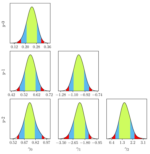
Figure 2: The same as in Fig. 1, except for the $y$-0, $y$-1, $y$-2 cases. See the text and Table 3 for details.

IV Observational constraints with the Padé cosmography

In the previous section, two types of ordinary cosmography are considered. As mentioned above, the $z$-cosmography might diverge at high redshift $z$. So, the $y$-cosmography was proposed as an alternative in the literature, which converges in the whole cosmic past $0\leq z<\infty$. However, there still exist several problems in the $y$-cosmography. In practice, the Taylor series should be truncated by throwing away the higher order terms, since it is difficult to deal with infinite series. So, the error of a Taylor approximation with lower order terms will become unacceptably large when $y=z/(1+z)$ is close to $1$ (say, when $z>9$). On the other hand, the $y$-cosmography cannot work well in the cosmic future $-1<z<0$. The Taylor series with respect to $y=z/(1+z)$ does not converge when $y<-1$ (namely $z<-1/2$), and it drastically diverges when $z\to-1$ (it is easy to see that $y\to-\infty$ in this case). Therefore, in Zhou:2016nik , we proposed some generalizations of cosmography inspired by the Padé approximant, which can avoid or at least alleviate the problems of ordinary cosmography.

The so-called Padé approximant can be regarded as a generalization of the Taylor series. For any function $F(x)$, its Padé approximant of order $(m,\,n)$ is given by the rational function Pade1892 ; Padewiki ; PadeTalk (see also e.g. Adachi:2011vu ; Gruber:2013wua ; Wei:2013jya ; Liu:2014vda ; Capozziello:2018jya ; Aviles:2014rma ; Capozziello:2017ddd )

$$F(x)=\frac{\alpha_{0}+\alpha_{1}x+\cdots+\alpha_{m}x^{m}}{1+\beta_{1}x+\cdots+\beta_{n}x^{n}}\,,$$ (16)

where $m$ and $n$ are both non-negative integers, and $\alpha_{i}$, $\beta_{i}$ are all constants. Obviously, it reduces to the Taylor series when all $\beta_{i}=0$. Actually in mathematics, a Padé approximant is the best approximation of a function by a rational function of given order Padewiki . In fact, the Padé approximant often gives a better approximation of the function than truncating its Taylor series, and it may still work where the Taylor series does not converge Padewiki .

One can directly parameterize the dimensionless luminosity distance based on the Padé approximant with respect to redshift $z$ Zhou:2016nik ,

$$D_{L}=\frac{H_{0}d_{L}}{c}=\frac{\alpha_{0}+\alpha_{1}z+\cdots+\alpha_{m}z^{m}}{1+\beta_{1}z+\cdots+\beta_{n}z^{n}}\,.$$ (17)

Following Zhou:2016nik , we consider a moderate order $(2,\,2)$ in this work, and then

$$D_{L}\equiv\frac{H_{0}d_{L}}{c}=\frac{\alpha_{0}+\alpha_{1}z+\alpha_{2}z^{2}}{1+\beta_{1}z+\beta_{2}z^{2}}\,.$$ (18)

Obviously, it can work well in the whole redshift range $-1<z<\infty$, including not only the past but also the future of the universe. In particular, it is still finite even when $z\gg 1$. In fact, this $D_{L}$ was confronted with Union2.1 SNIa data and Planck 2015 CMB data in Zhou:2016nik , and the parameters $\alpha_{0}$ and $\beta_{2}$ were found to be very close to $0$ even in the $3\sigma$ region. So, in the present work, it is safe to directly set

$$\alpha_{0}=\beta_{2}=0\,,$$ (19)

and then the free parameters are now $\alpha_{1}$, $\alpha_{2}$ and $\beta_{1}$. Note that in fact $\alpha_{0}=0$ is required by $d_{L}(z=0)=0$ theoretically. On the other hand, we can also expand $\gamma(z)$ as a Taylor series with respect to redshift $z$, namely $\gamma(z)=\gamma_{0}+\gamma_{1}\,z+\gamma_{2}\,z^{2}+...$. Again, we consider three cases, labeled as “ P-0 ”, “ P-1 ”, “ P-2 ”, in which $\gamma(z)$ is Taylor expanded up to zeroth, first, second orders, respectively.

Parameters	Case P-0	Case P-1	Case P-2
$\Omega_{m0}$	$0.3277_{-0.0210}^{+0.0210}{}_{-0.0403}^{+0.0428}{}_{-0.0523}^{+0.0570}$	$0.3366_{-0.0344}^{+0.0275}{}_{-0.0604}^{+0.0637}{}_{-0.0727}^{+0.0929}$	$0.3407_{-0.0351}^{+0.0291}{}_{-0.0623}^{+0.0647}{}_{-0.0750}^{+0.0911}$
$\alpha_{1}$	$0.9471_{-0.0329}^{+0.0328}{}_{-0.0631}^{+0.0670}{}_{-0.0820}^{+0.0899}$	$0.9362_{-0.0458}^{+0.0458}{}_{-0.0909}^{+0.0904}{}_{-0.1194}^{+0.1197}$	$0.9307_{-0.0458}^{+0.0458}{}_{-0.0883}^{+0.0916}{}_{-0.1141}^{+0.1219}$
$\alpha_{2}$	$1.0216_{-0.0442}^{+0.0442}{}_{-0.0863}^{+0.0880}{}_{-0.1129}^{+0.1163}$	$1.0083_{-0.0598}^{+0.0600}{}_{-0.1212}^{+0.1146}{}_{-0.1605}^{+0.1480}$	$1.0012_{-0.0581}^{+0.0581}{}_{-0.1147}^{+0.1154}{}_{-0.1493}^{+0.1517}$
$\beta_{1}$	$0.3329_{-0.0153}^{+0.0153}{}_{-0.0293}^{+0.0309}{}_{-0.0381}^{+0.0412}$	$0.3324_{-0.0161}^{+0.0148}{}_{-0.0295}^{+0.0313}{}_{-0.0384}^{+0.0415}$	$0.3321_{-0.0154}^{+0.0154}{}_{-0.0297}^{+0.0312}{}_{-0.0385}^{+0.0418}$
$\sigma_{8,\,0}$	$0.7615_{-0.0245}^{+0.0220}{}_{-0.0440}^{+0.0478}{}_{-0.0566}^{+0.0644}$	$0.7526_{-0.0337}^{+0.0338}{}_{-0.0662}^{+0.0684}{}_{-0.0864}^{+0.0921}$	$0.7480_{-0.0362}^{+0.0329}{}_{-0.0658}^{+0.0702}{}_{-0.0840}^{+0.0937}$
$\gamma_{0}$	$0.5462_{-0.0539}^{+0.0538}{}_{-0.1038}^{+0.1089}{}_{-0.1343}^{+0.1454}$	$0.5447_{-0.0544}^{+0.0543}{}_{-0.1051}^{+0.1097}{}_{-0.1374}^{+0.1470}$	$0.5562_{-0.0590}^{+0.0590}{}_{-0.1151}^{+0.1187}{}_{-0.1511}^{+0.1583}$
$\gamma_{1}$	N/A	$-0.0667_{-0.1908}^{+0.2110}{}_{-0.4122}^{+0.3801}{}_{-0.5546}^{+0.4923}$	$-0.2488_{-0.3854}^{+0.3858}{}_{-0.7665}^{+0.7622}{}_{-1.0127}^{+1.0016}$
$\gamma_{2}$	N/A	N/A	$0.2378_{-0.4540}^{+0.4531}{}_{-0.9190}^{+0.8788}{}_{-1.2341}^{+1.1400}$

Table 4: The mean with $1\sigma$, $2\sigma$, $3\sigma$ marginalized uncertainties of the model parameters for the cases with the Padé cosmography and $\gamma=\gamma_{0}$ (labeled as “ P-0 ”), $\gamma=\gamma_{0}+\gamma_{1}\,z$ (labeled as “ P-1 ”), $\gamma=\gamma_{0}+\gamma_{1}\,z+\gamma_{2}\,z^{2}$ (labeled as “ P-2 ”). See the text for details.

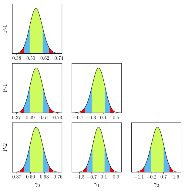
Figure 3: The same as in Fig. 1, except for the P-0, P-1, P-2 cases. See the text and Table 4 for details.

Since the Padé cosmography still works well at very high redshift $z\gg 1$ in contrast to the ordinary cosmography as mentioned above, in this section, we further use the latest CMB data in addition to the observational data mentioned in Sec. II. However, using the full data of CMB to perform a global fitting consumes a large amount of computation time and power. As a good alternative, one can instead use the shift parameter $R$ Bond:1997wr from CMB, which has been used extensively in the literature (including the works of the Planck and the WMAP Collaborations themselves). It is argued in e.g. Wang:2006ts ; Wang:2013mha ; Shafer:2013pxa that the shift parameter $R$ is model-independent and contains the main information of the observation of CMB. As is well known, the shift parameter $R$ is defined by Bond:1997wr ; Wang:2006ts ; Wang:2013mha ; Shafer:2013pxa

$$R\equiv\sqrt{\Omega_{m0}H^{2}_{0}}\,\left(1+z_{\ast}\right)d_{A}(z_{\ast})/c=\frac{\sqrt{\Omega_{m0}}\,D_{L}(z_{\ast})}{1+z_{\ast}}\,,$$ (20)

where the redshift of the recombination $z_{\ast}=1089.92$ from the Planck 2018 data Aghanim:2018eyx , and the angular diameter distance $d_{A}$ is related to the luminosity distance $d_{L}$ through $d_{A}=d_{L}(1+z)^{-2}$ (see e.g. the textbooks Weinberg1972 ). Here we adopt the value $R_{obs}=1.7502\pm 0.0046$ Chen:2018dbv derived from the Planck 2018 data. Thus, the corresponding $\chi^{2}$ from the latest CMB data is given by $\chi^{2}_{R}=(R_{\rm mod}-R_{obs})^{2}/\sigma_{R}^{2}$. Although the number of data points $\cal N$ and the number of free parameters $\kappa$ both increase by $1$, the degree of freedom $dof={\cal N}-\kappa$ is unchanged in this case. It is worth noting that the acoustic scale $l_{A}$, and $\Omega_{b}h^{2}$, the scalar spectral index $n_{s}$ are commonly used with the shift parameter $R$ in the literature, but they will introduce extra model parameters as mentioned above, and hence we do not use them here.

By using the latest observational data, we obtain the constraints on all the model parameters involved, and present them in Table 4, for the P-0, P-1, P-2 cases. In Fig. 3, we also present the 1D marginalized probability distributions of the parameters related to the growth index $\gamma$, namely $\gamma_{0}$, $\gamma_{1}$ and $\gamma_{2}$. In all cases, $\gamma_{0}\simeq 0.42$ is inconsistent with the latest observational data beyond $2\sigma$ C.L. (but it could be consistent in the $3\sigma$ region). On the other hand, in all cases, $\gamma_{0}\simeq 0.55$ is well consistent with the latest observational data within the $1\sigma$ region. Note that in all cases, a constant $\gamma=\gamma_{0}$ (namely $\gamma_{1}=0$ and $\gamma_{2}=0$) is well consistent with the latest observational data within the $1\sigma$ region (but see below).

V Conclusion and discussion

In this work, we consider the constraints on the growth index $\gamma$ by using the latest observational data. To be model-independent, we use cosmography to describe the cosmic expansion history, and also expand the general $\gamma(z)$ as a Taylor series with respect to redshift $z$ or $y$-shift, $y=1-a=z/(1+z)$. We find that the present value $\gamma_{0}=\gamma(z=0)\simeq 0.42$ (for most of viable $f(R)$ theories) is inconsistent with the latest observational data beyond $3\sigma$ C.L. in the 6 cases with the usual cosmography, or beyond $2\sigma$ C.L. in the 3 cases with the Padé cosmography. This result supports our previous work Yin:2018mvu . On the other hand, $\gamma_{0}\simeq 0.55$ (for dark energy models in GR) is consistent with the latest observational data at $1\sigma$ C.L. in 5 of the 9 cases under consideration, but is inconsistent beyond $2\sigma$ C.L. in the other 4 cases (while it is still consistent within the $3\sigma$ region). Therefore, we can say nothing firmly about $\gamma_{0}\simeq 0.55$. This result is still consistent with the reconstructed $\gamma(z)$ at $z=0$ obtained in our previous work Yin:2018mvu . A varying $\gamma$ with non-zero $\gamma_{1}$ and/or $\gamma_{2}$ is favored in the cases with the usual cosmography, while in the cases with the Padé cosmography, a constant $\gamma=\gamma_{0}$ (namely $\gamma_{1}=0$ and $\gamma_{2}=0$) can still be consistent with the latest observational data (but this might be artificial, see below).

It is of interest to compare the 9 cases considered here. We adopt several goodness-of-fit criteria used extensively in the literature to this end, such as $\chi^{2}_{min}/dof$, $P(\chi^{2}>\chi^{2}_{min})$ (see e.g. Wei:2006ut ; Wei:2007ws ), Bayesian Information Criterion (BIC) Schwarz:1978 and Akaike Information Criterion (AIC) Akaike:1974 , where the degree of freedom $dof={\cal N}-\kappa$, while $\cal N$ and $\kappa$ are the number of data points and the number of free model parameters, respectively. The BIC is defined by Schwarz:1978

$${\rm BIC}=-2\ln{\cal L}_{max}+\kappa\ln{\cal N}\,,$$ (21)

and the AIC is defined by Akaike:1974

$${\rm AIC}=-2\ln{\cal L}_{max}+2\kappa\,,$$ (22)

where ${\cal L}_{max}$ is the maximum likelihood. In the Gaussian cases, $\chi^{2}_{min}=-2\ln{\cal L}_{max}$. The difference in BIC or AIC between two models makes sense. We choose the P-0 case to be the fiducial model when we calculate $\Delta$BIC and $\Delta$AIC. In Table 5, we present $\chi^{2}_{min}/dof$, $P(\chi^{2}>\chi^{2}_{min})$, $\Delta$BIC and $\Delta$AIC for the 9 cases considered in this work. Clearly, the cases with $y$-cosmography are the worst, while the cases P-0 and $z$-2 are the best. In fact, the goodness-of-fit criteria for the cases P-0 and $z$-2 are fairly close. A caution should be mentioned here. All the criteria given in Table 5 are based on $\chi^{2}_{min}$, which are read from the output .likestats files of the CosmoMC program GetDist. However, as the CosmoMC Lewis:2002ah readme file puts it, “ file_-root.likestats gives the best fit sample model, its likelihood, and … Note that MCMC does not generally provide accurate values for the best-fit.” Keeping this in mind, we could say that the cases P-0 and $z$-2 are equally good, since their not so accurate $\chi^{2}_{min}$ are very close actually. In the P-0 case, the growth index $\gamma=\gamma_{0}$ is constant. However, in the $z$-2 case, $\gamma_{2}<0$ beyond $3\sigma$ C.L. (see Table 2 and Fig. 1), and hence the function $\gamma(z)$ is a parabola opening down, namely $\gamma$ increases and then decreases as redshift $z$ increases. There exists an arched structure in the moderate redshift range. This result is quite similar to the one of Yin:2018mvu . In Fig. 4, we show a demonstration of $\gamma=\gamma_{0}+\gamma_{1}\,z+\gamma_{2}\,z^{2}$ with $\gamma_{0}=0.6$, $\gamma_{1}=0.45$, $\gamma_{2}=-0.24$, which are all well within the $1\sigma$ regions of their observational constraints for the $z$-2 case (see Tabel 2 and Fig. 1).

Cases	$z$-0	$z$-1	$z$-2	$y$-0	$y$-1	$y$-2	P-0	P-1	P-2
$\chi^{2}_{min}$	1106.2202	1101.3110	1093.0770	1281.5972	1129.5110	1116.2714	1094.7438	1094.7268	1094.3310
$\cal N$	1127	1127	1127	1127	1127	1127	1128	1128	1128
$\kappa$	5	6	7	5	6	7	6	7	8
$\chi^{2}_{min}/dof$	0.9859	0.9824	0.9760	1.1422	1.0076	0.9967	0.9757	0.9766	0.9771
$P(\chi^{2}>\chi^{2}_{min})$	0.6257	0.6570	0.7120	0.0006	0.4233	0.5258	0.7143	0.7072	0.7028
$\Delta{\rm BIC}$	4.4438	6.5619	5.3552	179.8210	34.7619	28.5496	0	7.0112	13.6436
$\Delta{\rm AIC}$	9.4764	6.5672	0.3332	184.8530	34.7672	23.5276	0	1.9830	3.5872
Rank	6	5	2	9	8	7	1	3	4

Table 5: Comparing the 9 cases considered in the present work. See the text for details and caution.

It is worth noting that throughout this work, we always consider the growth index $\gamma$ as a Taylor series with respect to $z$ or $y$, namely $\gamma(z)=\gamma_{0}+\gamma_{1}\,z+\gamma_{2}\,z^{2}+...$, or $\gamma(y)=\gamma_{0}+\gamma_{1}\,y+\gamma_{2}\,y^{2}+...$ However, in Sec. IV, we parameterize the dimensionless luminosity distance $D_{L}$ by using the Padé approximant, and hence it can still work well at very high redshift $z\sim 1090$. Obviously, it is better to also parameterize the growth index $\gamma(z)$ by using the Padé approximant (we thank the referee for pointing out this issue). But the cost is expensive to do this. If we want to catch the arched structure in $\gamma(z)$, at least a Padé approximant of order $(2,\,2)$ is needed, which has 5 free parameters (n.b. Eq. (16)), and almost double the number of free parameters in a 2nd order Taylor series. So, in the P-2 case, the total number of free model parameters will be 10. It will consume significantly more computation power and time, but the corresponding constraints will be very loose. Therefore, we choose not to do this at a great cost. But one should be aware of the possible artificial results from this choice. For example, $\gamma(z)=\gamma_{0}+\gamma_{1}\,z+\gamma_{2}\,z^{2}$ will diverge at $z\sim 1090$, and hence the values of $\gamma_{1}$ and $\gamma_{2}$ tend to be zero to fit the high-$z$ CMB data in the P-1, P-2 cases (we thank the referee for pointing out this issue).

Some remarks are in order. First, the growth rate $f$ and then the growth index $\gamma$ for modified gravity scenarios (especially $f(R)$ theories) in principle are not only time-dependent but also scale-dependent (see e.g. Gannouji:2008wt ; Tsujikawa:2009ku ). However, as is shown in e.g. Gannouji:2008wt ; Tsujikawa:2009ku , the behavior of $\gamma$ is nearly scale-independent at low redshift $z\,\lower 3.22916pt\hbox{$\sim$}\hbox to0.0pt{\hss\raise 1.1625pt\hbox{$<$}}\,1$, and $\gamma_{0}=\gamma(z=0)$ is also nearly independent of scale. So, this issue does not change the main conclusions of the present work, although it may be studied carefully in the future work. Second, as is mentioned in the beginning of Sec. II, there exist other two approaches dealing with the growth history, which numerically solve the perturbation equations by using the code CAMB integrated in CosmoMC. We will also consider these approaches in the future work. Third, in the present work, we do not use some types of observational data (for example, the observational $H(z)$ data, and other kinds of BAO data) to avoid introducing extra model parameters. However, in principle, it is not terrible to do so, although the constraints might be loose and the calculations might be complicated. Finally, in this work, we only consider the Taylor series expansion of the growth index $\gamma$ up to 2nd order, and the usual cosmography up to 3rd order. In fact, one can also further consider higher orders in these cases. We anticipate that our main conclusions will not change significantly.

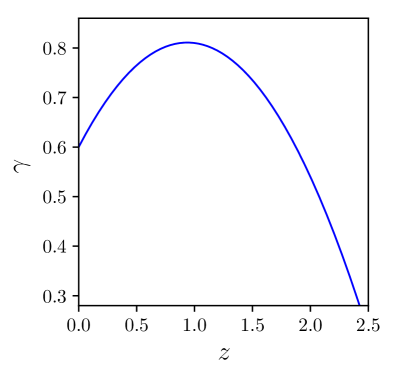
Figure 4: A demonstration of $\gamma=\gamma_{0}+\gamma_{1}\,z+\gamma_{2}\,z^{2}$ with $\gamma_{0}=0.6$, $\gamma_{1}=0.45$, $\gamma_{2}=-0.24$, which are all well within the $1\sigma$ regions of their observational constraints for the $z$-2 case (see Tabel 2 and Fig. 1).

References

- (1) A. G. Riess et al., Astron. J. 116, 1009 (1998) [astro-ph/9805201].
- (2) S. Perlmutter et al., Astrophys. J. 517, 565 (1999) [astro-ph/9812133].
- (3) M. Ishak, Living Rev. Rel. 22, no. 1, 1 (2019) [arXiv:1806.10122].
- (4) L. Amendola et al., Living Rev. Rel. 21, no. 1, 2 (2018) [arXiv:1606.00180].
- (5) A. Joyce, B. Jain, J. Khoury and M. Trodden, Phys. Rept. 568, 1 (2015) [arXiv:1407.0059].
- (6) T. Clifton, P. G. Ferreira, A. Padilla and C. Skordis, Phys. Rept. 513, 1 (2012) [arXiv:1106.2476].
- (7) V. Sahni and A. Starobinsky, Int. J. Mod. Phys. D 15, 2105 (2006) [astro-ph/0610026].
- (8) E. V. Linder, Phys. Rev. D 72, 043529 (2005) [astro-ph/0507263].
- (9) E. V. Linder and R. N. Cahn, Astropart. Phys. 28, 481 (2007) [astro-ph/0701317].
- (10) D. Huterer and E. V. Linder, Phys. Rev. D 75, 023519 (2007) [astro-ph/0608681].
-
(11)
Y. Wang,
JCAP 0805, 021 (2008)
[arXiv:0710.3885];
Y. Wang, arXiv:0712.0041 [astro-ph]. - (12) P. Zhang, M. Liguori, R. Bean and S. Dodelson, Phys. Rev. Lett. 99, 141302 (2007) [arXiv:0704.1932].
- (13) B. Jain and P. Zhang, Phys. Rev. D 78, 063503 (2008) [arXiv:0709.2375].
- (14) H. Wei, Phys. Lett. B 664, 1 (2008) [arXiv:0802.4122].
- (15) H. Wei and S. N. Zhang, Phys. Rev. D 78, 023011 (2008) [arXiv:0803.3292].
- (16) H. Wei, J. Liu, Z. C. Chen and X. P. Yan, Phys. Rev. D 88, 043510 (2013) [arXiv:1306.1364].
- (17) Z. Y. Yin and H. Wei, Sci. China Phys. Mech. Astron. 62, no. 9, 999811 (2019) [arXiv:1808.00377].
-
(18)
P. J. E. Peebles, Large-Scale Structure of the Universe,
Princeton University Press (1980);
P. J. E. Peebles, Astrophys. J. 284, 439 (1984). - (19) O. Lahav, P. B. Lilje, J. R. Primack and M. J. Rees, Mon. Not. Roy. Astron. Soc. 251, 128 (1991).
- (20) L. M. Wang and P. J. Steinhardt, Astrophys. J. 508, 483 (1998) [astro-ph/9804015].
- (21) A. Lue, R. Scoccimarro and G. D. Starkman, Phys. Rev. D 69, 124015 (2004) [astro-ph/0401515].
- (22) R. Gannouji, B. Moraes and D. Polarski, JCAP 0902, 034 (2009) [arXiv:0809.3374].
- (23) S. Tsujikawa et al., Phys. Rev. D 80, 084044 (2009) [arXiv:0908.2669].
- (24) A. Shafieloo, A. G. Kim and E. V. Linder, Phys. Rev. D 87, 023520 (2013) [arXiv:1211.6128].
- (25) S. Tsujikawa, Lect. Notes Phys. 800, 99 (2010) [arXiv:1101.0191].
-
(26)
S. Weinberg, Gravitation and Cosmology,
John Wiley & Sons, Inc., New York (1972);
S. Weinberg, Cosmology, Oxford University Press, Oxford (2008). -
(27)
M. Visser,
Class. Quant. Grav. 21, 2603 (2004)
[gr-qc/0309109];
M. Visser, Gen. Rel. Grav. 37, 1541 (2005) [gr-qc/0411131]. - (28) K. Bamba et al., Astrophys. Space Sci. 342, 155 (2012) [arXiv:1205.3421].
- (29) C. Cattoen and M. Visser, Phys. Rev. D 78, 063501 (2008) [arXiv:0809.0537].
- (30) V. Vitagliano, J. Q. Xia, S. Liberati and M. Viel, JCAP 1003, 005 (2010) [arXiv:0911.1249].
-
(31)
C. Cattoen and M. Visser,
gr-qc/0703122;
C. Cattoen and M. Visser, Class. Quant. Grav. 24, 5985 (2007) [arXiv:0710.1887];
M. Visser and C. Cattoen, arXiv:0906.5407 [gr-qc]. - (32) L. X. Xu and Y. Wang, Phys. Lett. B 702, 114 (2011) [arXiv:1009.0963].
- (33) J. Q. Xia et al., Phys. Rev. D 85, 043520 (2012) [arXiv:1103.0378].
- (34) M. J. Zhang, H. Li and J. Q. Xia, Eur. Phys. J. C 77, no. 7, 434 (2017) [arXiv:1601.01758].
-
(35)
P. K. S. Dunsby and O. Luongo,
Int. J. Geom. Meth. Mod. Phys. 13, 1630002 (2016)
[arXiv:1511.06532];
O. Luongo, G. B. Pisani and A. Troisi, Int. J. Mod. Phys. D 26, 1750015 (2016) [arXiv:1512.07076]. -
(36)
A. Aviles, C. Gruber, O. Luongo and H. Quevedo,
Phys. Rev. D 86, 123516 (2012)
[arXiv:1204.2007];
A. Aviles, A. Bravetti, S. Capozziello and O. Luongo, Phys. Rev. D 87, 044012 (2013) [arXiv:1210.5149];
A. Aviles, A. Bravetti, S. Capozziello and O. Luongo, Phys. Rev. D 87, 064025 (2013) [arXiv:1302.4871];
O. Luongo, Mod. Phys. Lett. A 26, 1459 (2011);
A. de la Cruz-Dombriz et al., JCAP 1612, 042 (2016) [arXiv:1608.03746]. - (37) Y. N. Zhou, D. Z. Liu, X. B. Zou and H. Wei, Eur. Phys. J. C 76, 281 (2016) [arXiv:1602.07189].
- (38) X. B. Zou, H. K. Deng, Z. Y. Yin and H. Wei, Phys. Lett. B 776, 284 (2018) [arXiv:1707.06367].
- (39) C. Gruber and O. Luongo, Phys. Rev. D 89, no. 10, 103506 (2014) [arXiv:1309.3215].
- (40) H. Wei, X. P. Yan and Y. N. Zhou, JCAP 1401, 045 (2014) [arXiv:1312.1117].
- (41) J. Liu and H. Wei, Gen. Rel. Grav. 47, no. 11, 141 (2015) [arXiv:1410.3960].
- (42) M. Adachi and M. Kasai, Prog. Theor. Phys. 127, 145 (2012) [arXiv:1111.6396].
- (43) S. Capozziello, Ruchika and A. A. Sen, Mon. Not. Roy. Astron. Soc. 484, 4484 (2019) [arXiv:1806.03943].
- (44) A. Aviles, A. Bravetti, S. Capozziello and O. Luongo, Phys. Rev. D 90, 043531 (2014) [arXiv:1405.6935].
- (45) S. Capozziello, R. D’Agostino and O. Luongo, JCAP 1805, no. 05, 008 (2018) [arXiv:1709.08407].
- (46) G. Gubitosi, F. Piazza and F. Vernizzi, JCAP 1302, 032 (2013) [arXiv:1210.0201].
- (47) J. Gleyzes, D. Langlois, F. Piazza and F. Vernizzi, JCAP 1308, 025 (2013) [arXiv:1304.4840].
- (48) P. A. R. Ade et al., Astron. Astrophys. 594, A14 (2016) [arXiv:1502.01590].
- (49) B. Hu, M. Raveri, N. Frusciante and A. Silvestri, Phys. Rev. D 89, 103530 (2014) [arXiv:1312.5742].
- (50) M. Raveri, B. Hu, N. Frusciante and A. Silvestri, Phys. Rev. D 90, 043513 (2014) [arXiv:1405.1022].
- (51) B. Hu, M. Raveri, N. Frusciante and A. Silvestri, arXiv:1405.3590 [astro-ph.IM].
- (52) G. B. Zhao, L. Pogosian, A. Silvestri and J. Zylberberg, Phys. Rev. D 79, 083513 (2009) [arXiv:0809.3791].
- (53) G. B. Zhao et al., Phys. Rev. D 81, 103510 (2010) [arXiv:1003.0001].
- (54) F. Simpson et al., Mon. Not. Roy. Astron. Soc. 429, 2249 (2013) [arXiv:1212.3339].
- (55) E. Macaulay, I. K. Wehus and H. K. Eriksen, Phys. Rev. Lett. 111, 161301 (2013) [arXiv:1303.6583].
- (56) T. Baker, P. G. Ferreira, C. D. Leonard and M. Motta, Phys. Rev. D 90, 124030 (2014) [arXiv:1409.8284].
- (57) S. F. Daniel et al., Phys. Rev. D 81, 123508 (2010) [arXiv:1002.1962].
- (58) A. Hojjati, L. Pogosian and G. B. Zhao, JCAP 1108, 005 (2011) [arXiv:1106.4543].
- (59) L. X. Xu, Phys. Rev. D 88, 084032 (2013) [arXiv:1306.2683].
-
(60)
A. Lewis and S. Bridle,
Phys. Rev. D 66, 103511 (2002)
[astro-ph/0205436];
http:cosmologist.info/cosmomc/ - (61) E. V. Linder, Phys. Rev. D 79, 063519 (2009) [arXiv:0901.0918].
- (62) F. Y. Wang, Astron. Astrophys. 543, A91 (2012).
- (63) J. E. Gonzalez, J. S. Alcaniz and J. C. Carvalho, JCAP 1604, 016 (2016) [arXiv:1602.01015].
- (64) J. E. Gonzalez, J. S. Alcaniz and J. C. Carvalho, JCAP 1708, 008 (2017) [arXiv:1702.02923].
- (65) S. Nesseris, G. Pantazis and L. Perivolaropoulos, Phys. Rev. D 96, 023542 (2017) [arXiv:1703.10538].
- (66) L. Kazantzidis and L. Perivolaropoulos, Phys. Rev. D 97, 103503 (2018) [arXiv:1803.01337].
- (67) D. M. Scolnic et al., Astrophys. J. 859, no. 2, 101 (2018) [arXiv:1710.00845].
-
(68)
The numerical data of the full Pantheon SNIa sample are available at
http:dx.doi.org/10.17909/T95Q4X
https:archive.stsci.edu/prepds/ps1cosmo/index.html -
(69)
The Pantheon plugin for CosmoMC is available at
https:github.com/dscolnic/Pantheon - (70) H. K. Deng and H. Wei, Eur. Phys. J. C 78, 755 (2018) [arXiv:1806.02773].
- (71) D. J. Eisenstein et al., Astrophys. J. 633, 560 (2005) [astro-ph/0501171].
- (72) C. Blake et al., Mon. Not. Roy. Astron. Soc. 418, 1707 (2011) [arXiv:1108.2635].
- (73) M. Kilbinger, Rept. Prog. Phys. 78, 086901 (2015) [arXiv:1411.0115].
- (74) C. Hikage et al., arXiv:1809.09148 [astro-ph.CO].
- (75) M. A. Troxel et al., Phys. Rev. D 98, 043528 (2018) [arXiv:1708.01538].
- (76) T. M. C. Abbott et al., Phys. Rev. D 98, 043526 (2018) [arXiv:1708.01530].
- (77) S. Joudaki et al., Mon. Not. Roy. Astron. Soc. 465, 2033 (2017) [arXiv:1601.05786].
- (78) H. Hildebrandt et al., Mon. Not. Roy. Astron. Soc. 465, 1454 (2017) [arXiv:1606.05338].
- (79) F. Köhlinger et al., Mon. Not. Roy. Astron. Soc. 471, 4412 (2017) [arXiv:1706.02892].
- (80) M. J. Jee et al., Astrophys. J. 824, 77 (2016) [arXiv:1510.03962].
- (81) E. van Uitert et al., Mon. Not. Roy. Astron. Soc. 476, 4662 (2018) [arXiv:1706.05004].
- (82) S. Joudaki et al., Mon. Not. Roy. Astron. Soc. 474, 4894 (2018) [arXiv:1707.06627].
- (83) N. Aghanim et al., arXiv:1807.06209 [astro-ph.CO].
- (84) J. Magana et al., Mon. Not. Roy. Astron. Soc. 476, 1036 (2018) [arXiv:1706.09848].
- (85) J. F. Zhang, Y. H. Li and X. Zhang, Phys. Lett. B 739, 102 (2014) [arXiv:1408.4603].
- (86) M. M. Zhao, J. F. Zhang and X. Zhang, Phys. Lett. B 779, 473 (2018) [arXiv:1710.02391].
-
(87)
H. Padé,
Ann. Sci. Ecole Norm. Sup. 9 (3), 1-93 (1892);
S. G. Krantz and H. R. Parks, A Primer of Real Analytic Functions, Birkhäuser (1992);
G. A. Baker, Jr. and P. Graves-Morris, Padé Approximants, Cambridge University Press (1996). - (88) http:en.wikipedia.org/wiki/Pade-approximant
-
(89)
http:www.scholarpedia.org/article/Pade-approximant
http:www-sop.inria.fr/apics/anap03/PadeTalk.pdf -
(90)
J. R. Bond, G. Efstathiou and M. Tegmark,
Mon. Not. Roy. Astron. Soc. 291, L33 (1997)
[astro-ph/9702100];
G. Efstathiou and J. R. Bond, Mon. Not. Roy. Astron. Soc. 304, 75 (1999) [astro-ph/9807103]. - (91) Y. Wang and P. Mukherjee, Astrophys. J. 650, 1 (2006) [astro-ph/0604051].
- (92) Y. Wang and S. Wang, Phys. Rev. D 88, 043522 (2013) [arXiv:1304.4514].
- (93) D. L. Shafer and D. Huterer, Phys. Rev. D 89, 063510 (2014) [arXiv:1312.1688].
- (94) L. Chen, Q. G. Huang and K. Wang, JCAP 1902, 028 (2019) [arXiv:1808.05724].
- (95) H. Wei and S. N. Zhang, Phys. Lett. B 644, 7 (2007) [astro-ph/0609597].
- (96) H. Wei and S. N. Zhang, Phys. Lett. B 654, 139 (2007) [arXiv:0704.3330].
- (97) G. Schwarz, Ann. Stat. 6, 461 (1978).
- (98) H. Akaike, IEEE Trans. Automatic Control 19, 716 (1974).
- (99) A. Viznyuk, S. Bag, Y. Shtanov and V. Sahni, Phys. Rev. D 98, 064024 (2018) [arXiv:1805.10405].
-
(100)
L. Amendola et al.,
Mon. Not. Roy. Astron. Soc. 449, 2845 (2015)
[arXiv:1412.3703];
T. Castro, M. Quartin and S. Benitez-Herrera, Phys. Dark Univ. 13, 66 (2016) [arXiv:1511.08695]. - (101) S. Basilakos and S. Nesseris, Phys. Rev. D 94, 123525 (2016) [arXiv:1610.00160].
- (102) S. Capozziello et al., Mon. Not. Roy. Astron. Soc. 476, 3924 (2018) [arXiv:1712.04380].
- (103) O. Luongo, Mod. Phys. Lett. A 28, 1350080 (2013).
-
(104)
S. Capozziello, R. D’Agostino and O. Luongo,
Gen. Rel. Grav. 51, 2 (2019)
[arXiv:1806.06385];
S. Capozziello, R. D’Agostino and O. Luongo, Gen. Rel. Grav. 49, 141 (2017) [arXiv:1706.02962].