Pulse-beam heating of deep atmospheric layers triggering their oscillations and upwards moving shocks that can modulate the reconnection in solar flares

Abstract

Aims. We study processes occurring after a sudden heating of the chromosphere at the flare arcade footpoints which is assumed to be caused by particle beams.

Methods. For the numerical simulations we adopt a 2-D magnetohydrodynamic (MHD) model, in which we solve a full set of the time-dependent MHD equations by means of the FLASH code, using the Adaptive Mesh Refinement (AMR) method.

Results. In the initial state we consider a model of the solar atmosphere with densities according to the VAL-C model and the magnetic field arcade having the X-point structure above, where the magnetic reconnection is assumed. We found that the sudden pulse-beam heating of the chromosphere at the flare arcade footpoints generates magnetohydrodynamic shocks, one propagating upwards and the second one propagating downwards in the solar atmosphere. The downward moving shock is reflected at deep and dense atmospheric layers and triggers oscillations of these layers. These oscillations generate the upwards moving magnetohydrodynamic waves that can influence the above located magnetic reconnection in a quasi-periodic way. Because these processes require a sudden heating in very localized regions in the chromosphere therefore they can be also associated with seismic waves.

1 Introduction

In solar flares oscillations are quite typical. They are observed in a broad range of the electromagnetic emission from radio, soft X-ray, hard X-ray, ultraviolet up to gamma-rays, see e.g. (Roberts et al., 1984; Fárník et al., 2003; Wang et al., 2005; Nakariakov et al., 2006, 2010). These oscillations are with periods from sub-seconds to tens of minutes (Mészárosová et al., 2006; Tan, 2008; Karlický et al., 2010; Kupriyanova et al., 2010; Huang et al., 2014; Nisticò et al., 2014). Many models of these observations have been proposed, see e.g. our last papers (Jelínek & Murawski, 2013; Guo et al., 2016; Jelínek et al., 2017) and for the review see e.g. the papers by (Pascoe, 2014; Nakariakov et al., 2016; McLaughlin et al., 2018).

It is commonly accepted that during the impulsive phase of solar flares, particle beams, which are accelerated by the magnetic reconnection in the low corona, propagate downwards along the legs of flare arcade and bombard dense chromospheric layers at their footpoints. Due to this bombardment the chromosphere at arcade footpoints is rapidly heated and the hard X-ray emission and magnetohydrodynamic shocks are generated (Brown, 1971; MacNeice et al., 1984; Mariska & Poland, 1985; Fisher et al., 1985a, b, c; Mariska et al., 1989; Karlický, 1990; Karlický & Henoux, 1992; Hawley & Fisher, 1994; Abbett & Hawley, 1999; Allred et al., 2005; Varady et al., 2014; Karlický & Jelínek, 2016).

In this paper we present new aspects of the above mentioned processes. Namely as will be shown in the following, a sudden and very localized heating of the chromosphere at the flare arcade footpoints triggers not only upwards and downwards moving shocks, but also the oscillations of deep atmospheric layers that then quasi-periodically generate the upwards moving shocks/waves which can modulate the primary-flare reconnection process located above. The reconnection rate is then quasi-periodically modulated and thus the oscillations found in the flare emissions can be explained. This scenario is a new alternative of the model presented by  Nakariakov et al. (2006), where the authors assumed a huge oscillating loop (resonator) generating waves which modulate a nearby flare magnetic reconnection.

The structure of the present paper is as follows. In Section 2 we present our numerical model, including the governing equations, initial equilibrium and perturbations. The results of numerical simulations and their interpretation are summarized in Section 3. Finally, we complete the paper by conclusions in the last Sect. 4.

2 Model

2.1 Governing equations

In our computer simulation we implement a gravitationally stratified solar atmosphere, according to VAL-C model, in which the plasma dynamics are described by the two-dimensional (2-D), time-dependent non-ideal (resistive) magnetohydrodynamic (MHD) equations. We solve the problem numerically with the use of FLASH code (Lee, 2013), where the MHD equations are formulated in conservative form as follows

$$\frac{\partial\varrho}{\partial t}+\nabla\cdot(\varrho\bm{\mathrm{v}})=0,$$ (1)

$$\frac{\partial\varrho\bm{\mathrm{v}}}{\partial t}+\nabla\cdot\left(\varrho\bm{\mathrm{v}}\bm{\mathrm{v}}-\bm{\mathrm{B}}\bm{\mathrm{B}}\right)+\nabla p_{*}=\varrho\bm{\mathrm{g}},$$ (2)

$$\frac{\partial\varrho E}{\partial t}+\nabla\cdot\left[\left(\varrho E+p_{*}\right)\bm{\mathrm{v}}-\bm{\mathrm{B}}(\bm{\mathrm{v}}\cdot\bm{\mathrm{B}})\right]=$$

$$=\varrho\bm{\mathrm{g}}\cdot\bm{\mathrm{v}}+\nabla\cdot(\bm{\mathrm{B}}\times(\eta\nabla\times\bm{\mathrm{B}})),$$ (3)

$$\frac{\partial\bm{\mathrm{B}}}{\partial t}+\nabla\cdot(\bm{\mathrm{v}}\bm{\mathrm{B}}-\bm{\mathrm{B}}\bm{\mathrm{v}})=-\nabla\times(\eta\nabla\times\bm{\mathrm{B}}),$$ (4)

$$\nabla\cdot\bm{\mathrm{B}}=0.$$ (5)

Here $\varrho$ is the mass density, $\bm{\mathrm{v}}$ is the flow velocity, $\bm{\mathrm{B}}$ is the magnetic field strength, $\bm{\mathrm{g}}=[0,-g_{\sun},0]$ is the gravitational acceleration with $g_{\sun}=274\leavevmode\nobreak\ \mathrm{ms^{-2}}$ and $\eta$ is the magnetic diffusivity taken constant throughout of the numerical box and corresponding to the relation $\eta=10^{9}T^{-3/2}$ (Priest, 2014) for the coronal temperature $T=10^{6}\leavevmode\nobreak\ \mathrm{K}$.

The total pressure $p_{*}$ is given by:

$$p_{*}=\left(p+\frac{B^{2}}{2\mu_{0}}\right),$$ (6)

$p$ is the fluid thermal pressure, $B$ is the magnitude of the magnetic field. The specific total energy $E$ in Eq. (2.1) is expressed as:

$$E=\epsilon+\frac{v^{2}}{2}+\frac{B^{2}}{2\mu_{0}\varrho},$$ (7)

where $\epsilon$ is the specific internal energy:

$$\epsilon=\frac{p}{(\gamma-1)\varrho},$$ (8)

with the adiabatic coefficient $\gamma=5/3$, $v$ is the magnitude of the flow velocity and $\mu_{0}=1.26\times 10^{-6}\leavevmode\nobreak\ \mathrm{Hm}^{-1}$ is the magnetic permeability of free space.

2.2 Initial state

For a still ($\bm{\mathrm{v}}=\bm{0}$) equilibrium, the Lorentz and gravity forces have to be balanced by the pressure gradient in the entire physical domain,

$$-\nabla p+\bm{\mathrm{j}}\times\bm{\mathrm{B}}+\varrho\bm{\mathrm{g}}=\bm{\mathrm{0}}.$$ (9)

Assuming a force-free magnetic field, $\bm{\mathrm{j}}\times\bm{\mathrm{B}}=\bm{\mathrm{0}}$, in the null-point the solution of the remaining hydrostatic equation yields

$$p_{\rm h}(y)=p_{0}\exp\left[-\int\limits_{y_{0}}^{y}\frac{1}{\Lambda(\tilde{y})}\mathrm{d}\tilde{y}\right],$$ (10)

$$\varrho(y)=\frac{p(y)}{g_{\sun}\Lambda(y)}.$$ (11)

Here

$$\Lambda(y)=\frac{k_{\mathrm{B}}T(y)}{\overline{m}g_{\sun}}$$ (12)

is the pressure scale-height which in the case of isothermal atmosphere represents the vertical distance over which the gas pressure decreases by a factor of $e\approx 2.7$, $k_{\mathrm{B}}=1.38\times 10^{-23}\leavevmode\nobreak\ \mathrm{J\cdot K^{-1}}$ is the Boltzmann constant and $\overline{m}=0.6\,m_{\mathrm{p}}$ is the mean particle mass ($m_{\mathrm{p}}=1.672\times 10^{-27}\leavevmode\nobreak\ \mathrm{kg}$ is the proton mass), $p_{0}\approx 10^{-2}\leavevmode\nobreak\ \mathrm{Pa}$ in Eq. (9) denotes the gas pressure at the reference level $y_{0}$. In our calculations we set and hold fixed $y_{0}=10\leavevmode\nobreak\ \mathrm{Mm}$. For the solar atmosphere we used the temperature profile derived by (Avrett & Loeser, 2008). At the top of the photosphere, which corresponds to the height of $y=0.5\leavevmode\nobreak\ \mathrm{Mm}$, the temperature is $T(y)=5700\leavevmode\nobreak\ \mathrm{K}$. At higher altitudes, the temperature falls down to its minimal value $T(y)=4350\leavevmode\nobreak\ \mathrm{K}$ at $y\approx 0.95\leavevmode\nobreak\ \mathrm{Mm}$. Higher up the temperature rises slowly to the height of about $y=2.7\leavevmode\nobreak\ \mathrm{Mm}$, where the transition region is located. Here the temperature increases abruptly to the value $T(y)=1.5\leavevmode\nobreak\ \mathrm{MK}$, at the altitude $y=10\leavevmode\nobreak\ \mathrm{Mm}$, which is typical for the solar corona.

The solenoidal condition, $\nabla\cdot\bm{\mathrm{B}}=0$, is identically satisfied with the use of the magnetic flux function, $\bm{\mathrm{A}}$, such as

$$\bm{\mathrm{B}}=\nabla\times\bm{\mathrm{A}}.$$ (13)

Specifically, to represent the non-potential null-point we use $\bm{\mathrm{A}}=[0,0,A_{z}]$, such as (Parnell et al., 1997; Jelínek et al., 2015)

$$A_{z}=\frac{1}{4}B_{\mathrm{0}}[(\mathcal{I}_{t}-\mathcal{I}_{z})y^{2}-(\mathcal{I}_{t}+\mathcal{I}_{z})x^{2}],$$ (14)

which gives us for magnetic field components

$$B_{x}(x,y)=\frac{B_{0}}{2}(\mathcal{I}_{t}-\mathcal{I}_{z})y$$ (15)

and

$$B_{y}(x,y)=\frac{B_{0}}{2}(\mathcal{I}_{t}+\mathcal{I}_{z})x.$$ (16)

Here $\mathcal{I}_{t}$ is the threshold current which only depends on the parameters associated with the potential part of the field and it is assumed to be a constant in our calculations. The parameter $\mathcal{I}_{z}$ is the magnitude of the current perpendicular to the plane of the null-point. Both $\mathcal{I}_{t}$ and $\mathcal{I}_{z}$ are free parameters which govern the magnetic field configuration, see Parnell et al. (1996) for more details. Magnetic field at the reference level is set and hold fixed as $B_{0}=10\leavevmode\nobreak\ \mathrm{G}$.

The equilibrium gas pressure and mass density are computed according to the following equations, see Solov’ev (2010):

$$p(x,y)=p_{\rm h}-\frac{1}{\mu_{0}}\left[\int\limits_{-\infty}^{x}\frac{\partial^{2}A}{\partial y^{2}}\frac{\partial A}{\partial x}\mathrm{d}x+\frac{1}{2}\left(\frac{\partial A}{\partial x}\right)^{2}\right],$$ (17)

$$\varrho(x,y)=\varrho_{\rm h}(y) + \frac{1}{\mu_{0}g_{\sun}}\Bigg{\{}\frac{\partial}{\partial{y}}\Bigg{[}\int\limits_{-\infty}^{x}\frac{\partial^{2}A}{\partial y^{2}}\frac{\partial A}{\partial x}\mathrm{d}x+$$ (18)

$$+ \frac{1}{2}\Bigg{(}\frac{\partial A}{\partial x}\Bigg{)}^{2}\Bigg{]}-\frac{\partial A}{\partial y}\nabla^{2}A\Bigg{\}}.$$

With the use of Eq. (14) in these general formulas we obtain the expressions for the equilibrium gas pressure (Jelínek et al., 2015)

$$p(x,y)=p_{h}(y)-\frac{B_{0}^{2}}{4\mu_{0}}\mathcal{I}_{z}(\mathcal{I}_{t}+\mathcal{I}_{z})x^{2}$$ (19)

and mass density

$$\varrho(x,y)=\varrho_{h}(y)+\frac{B_{0}^{2}}{2\mu_{0}g}\mathcal{I}_{z}(\mathcal{I}_{t}-\mathcal{I}_{z})y.$$ (20)

The initial state, showing the distribution of gas pressure in logarithmic scale and governing magnetic field (black lines) is illustrated in Fig. 1. The red line represents the separatrix.

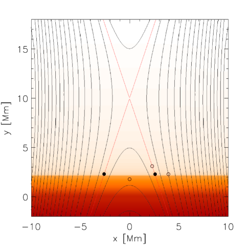
Figure 1: Sketch of the initial state in the equilibrium represented by the distribution of gas pressure (in logarithmic scale) and magnetic field lines (black lines) along with the separatrices (red lines). The initial pressure pulses are depicted as two black full circles at separatrices in the height $2.25\leavevmode\nobreak\ \mathrm{Mm}$ above the photosphere, i.e., at the transition region. Three unfilled black circles represent the detection points.

Generally, the terms expressing the radiative losses $R_{\mathrm{loss}}$, thermal conduction $T_{\mathrm{cond}}$ and heating $H$ should be added to the set of MHD equations. These terms are certainly important in building a realistic numerical model. However, at this stage when the wave and oscillatory processes are of primary interest, we neglect these terms.

2.3 Perturbations

To generate the initial perturbation pulse, at the start of the numerical simulation ($t=0\leavevmode\nobreak\ \mathrm{s}$), the equilibrium in the transition region (TR) is perturbed by the Gaussian pulse in the temperature (pressure) and has the following form

$$p=p_{0}\Bigg{\{}1+A_{\mathrm{p}}\sum_{i=1}^{2}\exp{\Bigg{[}-\frac{(x-x_{i}^{\mathrm{P}})^{2}+(y-y^{\mathrm{P}})^{2}}{\lambda^{2}}\Bigg{]}}\Bigg{\}},$$ (21)

where $p_{0}$ is the initial gas pressure, $A_{\mathrm{p}}$ is the initial amplitude of the pressure pulse, $\lambda$ is the size of the pressure pulse, $x_{i}^{\mathrm{P}}$ and $y^{\mathrm{P}}$ are the positions of the initial perturbation pulses. The perturbation points are placed in $x_{1}^{\mathrm{P}}=-2.58\leavevmode\nobreak\ \mathrm{Mm}$ and $x_{2}^{\mathrm{P}}=+2.58\leavevmode\nobreak\ \mathrm{Mm}$, respectively, with $y^{\mathrm{P}}=2.25\leavevmode\nobreak\ \mathrm{Mm}$ for both points, which corresponds to the position of TR.

2.4 Numerical code

For solution of the MHD equations (1)-(4) we use the FLASH code, which is well tested, fully modular, parallel, multiphysics, open science, simulation code that implements second- and third-order unsplit Godunov solvers with various slope limiters and Riemann solvers as well as adaptive mesh refinement (AMR) (Chung, 2002). The Godunov solver combines the corner transport upwind method for multi-dimensional integration and the constrained transport algorithm for preserving the divergence-free constraint on the magnetic field (Lee & Deane, 2009). We have used the minmod slope limiter and the Riemann solver e.g., (Toro, 2006). The main advantage of using AMR technique is to refine a numerical grid at steep spatial profiles while keeping a grid coarse at the places where fine spatial resolution is not essential. In our case, the AMR strategy is based on controlling the numerical errors in a gradient of mass density that leads to reduction of the numerical diffusion within the entire simulation region.

For our numerical simulations, we use a 2-D Eulerian box of its width $W=20\leavevmode\nobreak\ \mathrm{Mm}$ and height $H=20\leavevmode\nobreak\ \mathrm{Mm}$ as we set the numerical box as $(-10,10)\leavevmode\nobreak\ \mathrm{Mm}\times(-2,18)\leavevmode\nobreak\ \mathrm{Mm}$ in $x$ and $y$ direction, respectively. The spatial resolution of the numerical grid is determined with the AMR method. We use the AMR grid with the minimum (maximum) level of the refinement blocks set to 3 (7). The whole simulation region is covered by $2962$ blocks. Since every block consists $8\times 8$ numerical cells, this number of blocks corresponds to $189568$ numerical cells and the smallest spatial resolution is $\Delta x=\Delta y=3.9\leavevmode\nobreak\ \mathrm{km}$.

At all boundaries, we fix all plasma quantities to their equilibrium values using fixed-in-time boundary conditions, which lead only to negligibly small numerical reflections of incident wave signals.

3 Numerical results

Prior to run of the numerical simulation, we verified that the system is in equilibrium for the adopted grid resolution by running the system without any pressure pulse. After this control test, we launched in the system two symmetric pressure pulses with the amplitudes of $A_{\mathrm{p}}=10.0$ in the points at $x_{1,2}^{\mathrm{P}}$ and $y^{\mathrm{P}}$, see full black circles in Fig. 1. By this pressure pulse, the temperature at these points increased from the initial equilibrium value of $T_{\mathrm{eq}}\approx 0.17\leavevmode\nobreak\ \mathrm{MK}$ to the temperature $T\approx 1.7\leavevmode\nobreak\ \mathrm{MK}$.

In Figures 2 – 9 we show the results from our numerical simulations. For better readability and to see more details, Figs. 2 – 4 are shown within a range $(-5,5)\leavevmode\nobreak\ \mathrm{Mm}$ along $x-$direction.

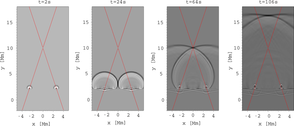
Figure 2: Temporal evolution of changes of the mass density $\Delta\varrho/\varrho_{0}$, at four different times, $t=2,26,64$ and $106\leavevmode\nobreak\ \mathrm{s}$. The initial pressure pulse was launched in TR on separatrices (solid red lines).

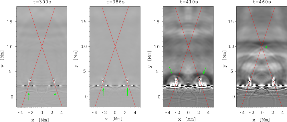
Figure 3: Temporal ime evolution of changes of the mass density $\Delta\varrho/\varrho_{0}$, at four different times, $t=300,386,410$ and $460\leavevmode\nobreak\ \mathrm{s}$, showing the secondary wave generated by the oscillation of the photosphere The wave is marked by the lightgreen arrows, the red line represents the separatrices.

In Figure 2 we show the time evolution of changes of the mass density $\Delta\varrho/\varrho_{0}$ for four different times, $t=2,26,64$ and $106\leavevmode\nobreak\ \mathrm{s}$, respectively. The crossing of the red lines indicates the X-point of the magnetic reconnection. At very early phase of this time evolution we can see that the shock wave, generated by the initial pressure pulse, propagates from both perturbation points symmetrically and at time $t=26\leavevmode\nobreak\ \mathrm{s}$ both wavefronts come across each other. Then both waves propagate towards the X-point ($x=0\leavevmode\nobreak\ \mathrm{Mm},y=10\leavevmode\nobreak\ \mathrm{Mm}$) which they reach at time $t=64\leavevmode\nobreak\ \mathrm{s}$. At time $t\approx 106\leavevmode\nobreak\ \mathrm{s}$ the waves come to the upper boundary of the presented region. It can also be seen that the waves propagate down to deeper layers of the solar atmosphere. These waves are partially remain in the photosphere and deeper layers of solar body and they are also partially reflected with lower energy back, towards the higher altitudes in the solar atmosphere, which is clearly seen in Fig. 3.

In Figure 3 we present the time evolution of changes of the mass density at later times, mainly at $t=300,386,410\leavevmode\nobreak\ \mathrm{s}$ and $t=460\leavevmode\nobreak\ \mathrm{s}$. We can see here the wave reflected from the photosphere ($y=0\leavevmode\nobreak\ \mathrm{Mm}$) as well as the waves propagating down to even deeper layers and reflected later; see also last two right panels of Fig. 2 for times $t=64\leavevmode\nobreak\ \mathrm{s}$ and $t=106\leavevmode\nobreak\ \mathrm{s}$. The reflected waves are marked by lightgreen arrows. The figure at $t=300\leavevmode\nobreak\ \mathrm{s}$ shows the wave shortly after the reflection from the photosphere. At time $t=386\leavevmode\nobreak\ \mathrm{s}$ the reflected wave reaches the TR. After that time the wave continues in propagation to higher layers of the solar atmosphere, where we show two wavefronts at the time $t=410\leavevmode\nobreak\ \mathrm{s}$. The last shot presents, the wave reaching the X-point at time $t=460\leavevmode\nobreak\ \mathrm{s}$.

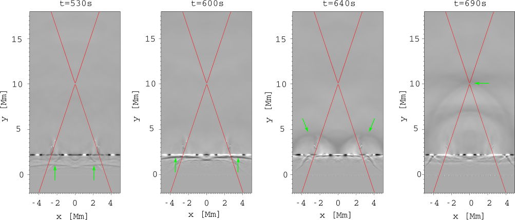
Figure 4: Temporal evolution of changes of the mass density $\Delta\varrho/\varrho_{0}$, at four different times, $t=530,600,640$ and $690\leavevmode\nobreak\ \mathrm{s}$, showing the second wave generated by the oscillation of the photosphere The wave is marked by the lightgreen arrows, the red line represents the separatrices.

Fig. 4 presents again the time evolution of relative change of mass density for different times $t=530,600,640\leavevmode\nobreak\ \mathrm{s}$ and $t=690\leavevmode\nobreak\ \mathrm{s}$. Similarly as in previous Figure 3, we can see here two waves triggered by oscillating photosphere ($t=530\leavevmode\nobreak\ \mathrm{s}$), whereas later in time $t=600\leavevmode\nobreak\ \mathrm{s}$ the waves reach the TR. At time $t=640\leavevmode\nobreak\ \mathrm{s}$ both wavefronts reach each other and continue in propagation higher to the solar atmosphere. At time $t=690\leavevmode\nobreak\ \mathrm{s}$ they cross the X-point at height $10\leavevmode\nobreak\ \mathrm{Mm}$. The most important aspect of this set of pictures is that the initial pressure pulse triggers oscillations of the photosphere and thus generating waves propagating upwards, where they can modulate quasi-periodically the process of the flare magnetic reconnection.

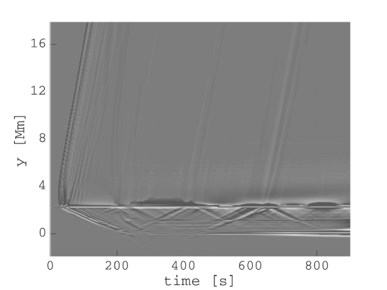
Figure 5: The time-space plot showing the evolution of relative mass density change $\Delta\varrho/\varrho_{0}$ along the $y$-axis of symmetry of the magnetic structure; $x=0\leavevmode\nobreak\ \mathrm{Mm}$.

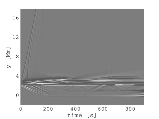
Figure 6: The time-space plot showing the evolution of relative mass density change $\Delta\varrho/\varrho_{0}$ along the $y$-axis passing the perturbation point at $x=2.58\leavevmode\nobreak\ \mathrm{Mm}$.

In Figs. 5 and 6 we show the time-space plot of an evolution of the relative change of mass density $\Delta\varrho/\varrho_{0}$ along the $y$-axis for two values of $x$. In Fig. 5 it is along the axis of the symmetry of the magnetic structure, i.e. for $x=0\leavevmode\nobreak\ \mathrm{Mm}$, whereas Fig. 6 shows the plot through the perturbation point at $x=2.58\leavevmode\nobreak\ \mathrm{Mm}$. In both figures, at the beginning, we can see two shocks (from two spatially separated pulses) propagating upwards and downwards to higher and deeper layers of the solar atmosphere, respectively.

Arrival of the shocks is delayed because of the distance from the point of perturbation. The first shock propagates from the nearby perturbation point and the second one from the more distant perturbation point. The vertical velocity and the Mach number of the shock propagating upwards are $v_{\mathrm{up}}\approx 0.18\leavevmode\nobreak\ \mathrm{Mm\cdot s^{-1}}$ and $M\approx$ 1.1 and those of the shock propagating downwards are $v_{\mathrm{down}}\approx 0.011\leavevmode\nobreak\ \mathrm{Mm\cdot s^{-1}}$ and $M\approx$ 1.5. The shock propagating to deeper layers of the solar atmosphere is partially reflected at time around $t\approx 200\leavevmode\nobreak\ \mathrm{s}$ and changes to waves. Some waves also propagate below the photosphere to locations, where they are later reflected. The wave above the photosphere reflects several times between TR and photosphere, and partially penetrates through TR and propagates upwards into the solar corona. Figure 6 is added for comparison. Here, the first shock starts without any delay, because this plot presents an evolution along the line which comes through the perturbation point.

In Figure 7 we show the time evolution of relative change of the mass density in the detection point located at the axis of the symmetry of the magnetic structure at $y=1.8\leavevmode\nobreak\ \mathrm{Mm}$. (For the position of detection points, see Figure 1.) This figure presents an another view on shocks (two first peaks) and waves below TR.

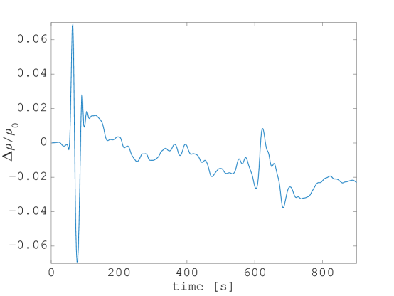
Figure 7: The time evolution of relative mass density change $\Delta\varrho/\varrho_{0}$ in the detection point $x=0\leavevmode\nobreak\ \mathrm{Mm}$ and $y=1.8\leavevmode\nobreak\ \mathrm{Mm}$.

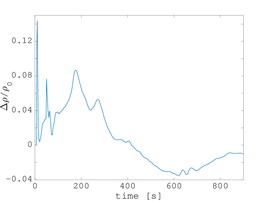
Figure 8: The time evolution of relative mass density change $\Delta\varrho/\varrho_{0}$ at the point $x=2.2\leavevmode\nobreak\ \mathrm{Mm}$ and $y=3.0\leavevmode\nobreak\ \mathrm{Mm}$.

In Fig. 8 we present again the time evolution of relative changes of the mass density $\Delta\varrho/\varrho_{0}$, but for the point close to the initial perturbation point, $x=2.2\leavevmode\nobreak\ \mathrm{Mm}$ and $y=3\leavevmode\nobreak\ \mathrm{Mm}$. This figure shows that during the pulse heating not only shocks are generated, but also the plasma is evaporated. We can see that after first strong peak at $t=10\leavevmode\nobreak\ \mathrm{s}$, which corresponds to the shock generated in the nearby perturbation point, the second peak produced by the shock from the distant perturbation point appears at $t=50\leavevmode\nobreak\ \mathrm{s}$. This second peak is is approximately twice ($\Delta=0.1436/0.7637$) lower than the first one. Then at $t=166\leavevmode\nobreak\ \mathrm{s}$ we observe the peak which is comparable with the previous one, but it is much broader. This peak shows an arrival of the evaporated plasma from the nearby perturbation point to the detection one, see also indication of the plasma evaporation in Fig. 2, last two panels for times $t=64$ and $106\leavevmode\nobreak\ \mathrm{s}$.

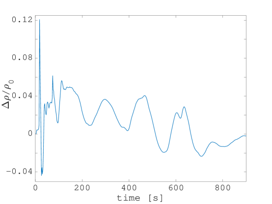
Figure 9: The time evolution of relative mass density change $\Delta\varrho/\varrho_{0}$ at the point $x=4.0\leavevmode\nobreak\ \mathrm{Mm}$ and $y=2.25\leavevmode\nobreak\ \mathrm{Mm}$.

The last Figure 9 shows the time evolution of the density variation at the point $x=4.0\leavevmode\nobreak\ \mathrm{Mm}$ and $y=2.25\leavevmode\nobreak\ \mathrm{Mm}$, which is located at the same altitude in TR as the perturbation point, but out of it. This figure shows the wave propagating from the perturbation point through TR. This wave can correspond to the waves observed sometimes in $H_{\alpha}$ or UV.

4 Conclusions

In this paper we numerically study shocks triggered by pressure pulses launched in the transition region and consequently generated oscillations of deep atmospheric layers and waves propagating upwards which can modulate quasi-periodically the magnetic reconnection in solar flares. The model is two-dimensional considering gravitationally stratified solar atmosphere with real temperature distribution according to the VAL-C model.

The processes shown in this paper represent a new possibility how to explain some periodicity of solar flare emissions. It is a new alternative to the model with the resonating loop presented by  Nakariakov et al. (2006).

A question arises if there are some observational evidence that oscillations of deep layers of the solar atmosphere produce upwards propagating magnetoacoustic shock/waves modulating the magnetic reconnection and thus periodically varying flare emissions.

From our computations it is evident that the oscillations of deep layers are triggered by a very localized and strong pulse beam heating. The same process was also proposed for generating of the seismic waves (Kosovichev & Zharkova, 1998; Zharkova & Zharkov, 2007). Thus, we expect that the flares associated with the seismic waves could be also connected with the processes presented in this paper. We plan to analyze this possibility in a future work.