Learning Triggers for Heterogeneous Treatment Effects

Abstract

The causal effect of a treatment can vary from person to person based on their individual characteristics and predispositions. Mining for patterns of individual-level effect differences, a problem known as heterogeneous treatment effect estimation, has many important applications, from precision medicine to recommender systems. In this paper we define and study a variant of this problem in which an individual-level threshold in treatment needs to be reached, in order to trigger an effect. One of the main contributions of our work is that we do not only estimate heterogeneous treatment effects with fixed treatments but can also prescribe individualized treatments. We propose a tree-based learning method to find the heterogeneity in the treatment effects. Our experimental results on multiple datasets show that our approach can learn the triggers better than existing approaches.

Introduction

Developing optimal precision treatments for diverse populations of interest can lead to more effective public policies (?), medical decisions (?; ?), recommender systems (?), and more (?). Treatment effects, also known as causal effects, assess the outcome response difference between applying a treatment to a unit and not applying one. Heterogeneous treatment effect (HTE) estimation refers to finding subsets in a population of interest for which the causal effects are different from the effects of the population as a whole (?). For example, if the treatment is a drug with potential adverse reactions, doctors may want to prescribe it only to those people who would benefit from it the most. Additionally, HTE analysis allows the discovery of subpopulations that can react adversely to a treatment and should avoid the treatment altogether. HTE can be studied as part of the post-analysis of running a controlled experiment or through observational data.

Supervised machine learning techniques have been adapted to the problem of HTE estimation (?; ?; ?; ?; ?) and the closely related problem of finding individualized treatment regimes which aims to find the best individual treatment assignment (?; ?; ?; ?; ?). Most of them rely on recursive partitioning using interpretable tree-based methods, such as decision lists (?), decision trees (?; ?; ?; ?; ?) and random forests (?; ?; ?). Some of the splitting criteria include highest parameter instability (?), t-statistic for the test of no difference between splits (?) and penalizing splits with high variance (?). In (?), an impurity measure is developed to measure risk of treatments in a partition. There are also other methods that rely on clustering (?) or propensity scores (?).

In many realistic scenarios, the treatment is an ordinal (or monotonously increasing continuous) variable, rather than a binary one, and the effect depends on the amount of treatment. For example, a clinician might be interested to understand the minimum number of days (the trigger) that patients with certain characteristics need to take a medication, in order to be cured (the effect). Or, a company might be interested in offering a personalized discount where the threshold is the minimum discount needed to trigger a customer with given characteristics to buy a product. Then, the goal becomes finding the threshold that maximizes the expected outcome for each discovered subpopulation where the subpopulation is characterized by its set of equal or similar attributes. To the best of our knowledge, none of the existing work addresses this problem which is the focus of our work.

We formalize this problem under the name trigger-based HTE estimation and develop a learning procedure that enables the discovery of individual-level thresholds for triggering an effect. In essence, we turn an ordinal treatment problem into a binary treatment one where the treatment threshold is learned. For each subpopulation, the treatment effect refers to the average difference between the outcomes for the individuals in the subpopulation whose treatment is below the threshold and those who are above the threshold. A key assumption here is that the subpopulation that has received treatment above the threshold represents the same underlying distribution as the subpopulation below the threshold. Trigger-based HTE estimation is closely related to estimating dose-response curve used in medical fields for estimating effects of diet (?) and survival analysis (?). In contrast, our method discovers subpopulations with heterogeneous triggers and effects.

Figure 1: A small tree illustrating triggers for HTE. The right most path reads: “If a person is male, started smoking younger than 19”, the average effect of smoking on medical expenditures is 0.642, for more than 3 $\log(\text{packyears})$.

Our proposed algorithm builds upon previous work on causal trees (?) which recursively partition a population using a decision tree-like approach. There are two main challenges to learning trigger-based HTE that have not been addressed by previous work on causal trees. First, a learning algorithm needs to be able to find effects that are robust and can generalize to unseen data. Second, trigger-based HTE requires simultaneous learning of population-level triggers and population HTE.

We propose a greedy algorithm with a novel scoring function that separates the full population into partitions with different effects. To address the first challenge, we treat the causal effects in different possible populations as hyperparameters that need to be estimated from a validation dataset. Our node-splitting criterion learns to generalize to unseen data by introducing a penalty on a model’s ability to estimate the conditional average causal effect. To address the second challenge, we search for treatment value thresholds that trigger the highest effects when binned into binary treatment and control groups based on that threshold.

Our main contributions include:

• Framing a new problem of practical interest: trigger-based HTE estimation;

• Developing the first method for discovering groups with trigger-based HTE;

• Utilizing trigger-based HTE estimation with causal trees for prescribing individualized treatments;

• Enabling causal effect generalization in causal tree learning through an appropriate node-splitting penalty;

• Discovering HTE with significantly lower error rates compared to existing baselines.

To illustrate the trigger-based HTE groups that our method can discover, we show a simple example in Fig. 1. The data is from the 1987 National Medical Expenditures Survey (NMES) (?). The treatment is amount of smoking (in $\log(packyears)$) and the effect is medical expenditures (in $\log(cost)$). The first splitting feature is gender, where the left path is true (female) and the right path is false (male). One example of a path in the tree is the right-most path: if a person is male and started smoking younger than 19 years old, then smoking more than $\log(packyears)$ leads to the highest difference in treatment effects compared to people with the same characteristics who smoked less, a $64.2\%$ increase in medical expenditures.

Preliminaries

First, we will present some background and definitions for causal inference, including assumptions needed for inferring treatment effects in observational data. Then, we present the heterogeneous treatment effect estimation problem. Finally, we briefly describe the causal tree approach proposed by (?).

Causal Inference

Suppose dataset $S$ has $N$ units which are independently and identically distributed (i.i.d.). For a unit $s_{i},(i=1,\dots,N)$, there are a pair of potential outcomes, $Y_{i}(0),Y_{i}(1)$. The individual causal effect (ICE) is defined as $\tau_{i}=Y_{i}(1)-Y_{i}(0)$, the difference in potential outcomes following the Rubin Causal Model (?) Define the indicator for treatment group assignment as $T_{i}\in\{0,1\}$, where $T_{i}=0$ and $T_{i}=1$ indicates that unit $s_{i}$ is in the control or treatment group, respectively. Traditionally, we cannot observe the outcome when treated and outcome when not treated simultaneously. The actual observed outcome is defined as:

$$Y_{i}^{\text{obs}}=Y_{i}(T_{i})=\begin{cases}Y_{i}(0),&\text{if $T_{i}=0$,}\\ Y_{i}(1),&\text{if $T_{i}=1$.}\end{cases}$$ (1)

We assume the potential outcome of one unit should not be affected by treatment assignment of other units (the stable unit treatment value assumption (SUTVA) (?)). We maintain the assumption of unconfoundedness (?), given as: $T_{i}\perp\left(Y_{i}(0),Y_{i}(1)\right)\mid X_{i}.$

Heterogeneous treatment effect estimation

The main focus of heterogeneous causal inference is to estimate the conditional average treatment effect (CATE) based on a set of features (?). The CATE is defined as: $\tau(x)\equiv\mathbb{E}\left[Y_{i}(1)-Y_{i}(0)|X_{i}=\bm{x}\right].$ The goal is to obtain accurate estimates $\hat{\tau}(x)$ for the CATE $\tau(x)$, which are based on a partitioning of the feature space.

Consider the feature space $\mathcal{X}\subset\mathbb{R}^{d}$ (we would like to note that we make this assumption for simplicity of exposition but our algorithms can easily be adapted for discrete features as well). A dataset $S$ consists of triples $S=\{(\bm{X}_{i},Y_{i},T_{i})\colon\bm{X}_{i}\in\mathcal{X}\}$ where $\bm{X}_{i}$ is the feature vector, $Y_{i}$ is the outcome or response, and $T_{i}$ is the binary indicator of treatment group assignment for unit $s_{i}$. A partitioning of the feature space into $L$ partitions is defined as $\mathcal{X}=\mathcal{X}_{1}\cup\dots\cup\mathcal{X}_{L}$, where $\mathcal{X}_{\ell}\cap\mathcal{X}_{\ell^{\prime}}=\emptyset$ for all $\ell\neq\ell^{\prime}$. The set of examples corresponding to partition $\mathcal{X}_{\ell}$ is $S_{\ell}=\{(\bm{X}_{i},Y_{i},T_{i})\colon X_{i}\in\mathcal{X}_{\ell}\}$.

The conditional mean for treatment and control in partition $\mathcal{X}_{\ell}$ is defined as:

$$\hat{\mu}_{t}(S_{\ell})=\frac{1}{N_{\ell_{1}}}\sum_{T_{i}=t,i\in S_{\ell}}Y_{i},$$ (2)

where $t\in\{0,1\}$, $\hat{\mu}_{1}$ and $\hat{\mu}_{0}$ are the conditional means for treatment and control groups in the partition, and $N_{\ell_{1}}$ and $N_{\ell_{0}}$ are the number of units in treatment and control groups in the partition, respectively. The average causal effect (ACE) $\hat{\tau}$ for partition $\mathcal{X}_{\ell}$ is defined as:

$$\hat{\tau}(S_{\ell})=\hat{\mu}_{1}(S_{\ell})-\hat{\mu}_{0}(S_{\ell}),$$ (3)

When performing estimation on a new set of data, say $S^{\text{te}}$, the test examples are matched to the correct partition given the features. Given an example $s_{j}\in S^{\text{te}}$ in partition $\ell$, the estimated ICE for unit $s_{j}$ is given by the ACE for $S_{\ell}$ as (3).

Objective function

The goal of HTE estimation is to partition the feature space, so that heterogeneity is found. Similar to (?), we define a partition measure that captures the magnitude in ACE for the partition: $F(S_{\ell})=N_{\ell}\cdot\hat{\tau}^{2}(S_{\ell})$, where $N_{\ell}=\lvert S_{\ell}\rvert$ is the number of samples in partition $\ell$.

To find subgroups for HTE, we wish to partition the feature space, so that the sum of all partition measures is maximized. For a feature space $\mathcal{X}$, the objective is to maximize the sum of partition measures $F$ across $L$ partitions:

$$\operatorname*{max}_{S_{1},\dots,S_{L}} \sum_{i=1}^{L}F(S_{i}),$$ (4)

s.t. $$\mathcal{X}=\mathcal{X}_{1}\cup\dots\cup\mathcal{X}_{L},$$

$$\mathcal{X}_{\ell}\cap\mathcal{X}_{\ell^{\prime}}=\emptyset,\;\ell\neq\ell^{\prime}$$

To reach this objective for the trigger-based HTE estimation, we need to optimize partition splits both based on features and possible feature threshold splits.

Recursive partitioning through causal trees

Trees are popular for HTE estimation (?; ?; ?). Each partition is represented by a path in the tree, similarly to decision trees. Trees are built in a greedy manner to maximize a $F$ from each node split. This results in locally optimizing the objective (4) as splitting criteria. Given a node $\ell$ that needs to be partitioned into two child nodes $\ell_{1},\ell_{2}$, the algorithm finds the split that maximizes $F$ for the two children:

$$\operatorname*{max}_{S_{\ell_{1}},S_{\ell_{2}}}F(S_{\ell_{1}})+F(S_{\ell_{2}})$$ (5)

such that $\mathcal{X}_{\ell}=\mathcal{X}_{\ell_{1}}\cup\mathcal{X}_{\ell_{2}}$ and $\mathcal{X}_{\ell_{1}}\cap\mathcal{X}_{\ell_{2}}=\emptyset$. A simple method for building a tree is to directly use this splitting, called the adaptive approach, which we denote as CT-A (?). The entire training set is used to build the tree and estimate causal effects.

A penalty can be introduced to the splitting criteria (?). This approach, called the honest approach, denoted as CT-H, is separated into two stages: tree-building and estimation. The data is split into a training and estimation sample, denoted by $S^{\text{tr}}$ and $S^{\text{est}}$, respectively. $S^{\text{tr}}$ is used for tree building and $S^{\text{est}}$ is used for estimation.

Triggers for HTE

When there is a treatment value threshold (e.g., minimum number of days to take a medication) that triggers an effect (e.g., to be cured), the partitions will depend on the optimal thresholds for each subpopulation. Let $t_{i}\in\mathbb{R}$ be the amount of treatment (e.g., number of days to take a medication) corresponding to each unit $s_{i}$. We define the trigger $\theta_{\ell}$ of a population $S_{\ell}$ as the threshold that splits $S_{\ell}$ into two subpopulations $S_{\ell_{1}}$ and $S_{\ell_{0}}$ in a way that optimizes the treatment effect for $S_{\ell}$:

$$\operatorname*{arg\,max\,\,}_{\theta_{\ell}}\hat{\mu}_{1}(S_{\ell_{1}})-\hat{\mu}_{0}(S_{\ell_{0}})$$ (6)

such that $S_{\ell}=S_{\ell_{1}}\cup S_{\ell_{0}}$, $S_{\ell_{1}}\cap S_{\ell_{0}}=\emptyset$, where $T_{i}=1$ if $t_{i}\geq\theta_{\ell}$ and $T_{i}=0$ otherwise. While we define the treatment as a real variable, threshold-based triggers also apply to treatments that are ordinal discrete values. Like in the non-trigger case, a key assumption here is that $S_{\ell_{1}}$ and $S_{\ell_{0}}$ represent the same underlying distribution and each unit $s_{i}\in S_{\ell}$ is equally likely to be assigned to each subgroup ($T_{i}\perp\left(Y_{i}(0),Y_{i}(1)\right)\mid X_{i}$).

Learning HTE

Next, we present our general approach to learning HTE, that applies to both discrete and trigger treatments. We explain in detail the specific requirements for the trigger case.

Algorithm 1 Learning trigger-based causal trees

1:Training set $S$, validation size $\rho$, indicator for measure $B$ ($B=1$ if binary, $B=0$ if trigger-based)

2:The root of the causal tree

3:$S^{\text{tr}},S^{\text{val}}$ = split($S$, split size=$\rho$)

4:root.F $\leftarrow$ PartitionMeasure($S,B$) {e.g. equation (9)}

5:root.S $\leftarrow S^{\text{tr}}$ {The sample at root node}

6:return Train(root)

7:function Train(currentNode)

8:     $S_{\ell}\leftarrow$ currentNode.S

9:     bestPartition $\leftarrow-\infty$

10:     for each feature split $\mathcal{X}_{\ell_{1}},\mathcal{X}_{\ell_{2}}$ do

11:         leftPartition = PartitionMeasure($S_{\ell_{1}},B$)

12:         rightPartition = PartitionMeasure($S_{\ell_{2}},B$)

13:         if leftPartition + rightPartition $>$ bestPartition 

14:              bestPartition = leftPartition + rightPartition               

15:     if bestPartition $>$ currentNode.F 

16:         left.F, left.S $\leftarrow$ leftPartition, $S_{\ell_{1}}$

17:         right.F, right.S $\leftarrow$ rightPartition, $S_{\ell_{2}}$

18:         currentNode.left $\leftarrow$ Train(left)

19:         currentNode.right $\leftarrow$ Train(right)

20:     else

21:         return currentNode      

22:function PartitionMeasure($S_{\ell}$, $B$)

23:     if $B==1$ { indicates no trigger } 

24:         return $F_{C}(S_{\ell})$

25:     else

26:         $\theta_{\ell}\leftarrow\emptyset$; {denotes the trigger}

27:         $v_{\ell}\leftarrow-\infty$; {$v$ is the best partition measure}

28:         $\mathcal{T}=\{t_{i}\colon t_{i}\in S_{\ell}\}$

29:         for each $t_{j}\in\mathcal{T}$ do

30:              $S_{\ell_{1}}=\{(\bm{X}_{i},Y_{i},T_{i})\colon T_{i}\geq t_{j}\}$

31:              $S_{\ell_{0}}=\{(\bm{X}_{i},Y_{i},T_{i})\colon T_{i}<t_{j}\}$

32:              temp = $F(S_{\ell_{1}}\cup S_{\ell_{0}})$

33:              if temp $>v_{\ell}$ 

34:                  $v_{\ell},\;\theta_{\ell}$ $\leftarrow$ temp, $t_{j}$                             

35:     return $v_{\ell},\theta_{\ell}$

Effect estimation

The formulation given previously may not be optimal on unseen test data. In contrast to (?), we propose a different splitting criterion by introducing the idea of a validation set to find splits that generalize well to unseen data. For our approach, we clearly separate a training, validation, and testing sample for training and evaluation. Additionally, we jointly optimize generalizability using training and validation in a one-stage tree-building process.

For a dataset $S$, we define the training, validation and testing samples as $S^{\text{tr}}$, $S^{\text{val}}$, and $S^{\text{te}}$. We build the tree on the training portion, while penalizing generalization ability based on the validation set. Our method estimates effects on the training sample and penalizes estimations that do not match a validation set by introducing a penalty or cost.

Let $\tilde{\tau}(S_{\ell}^{\text{tr}})$ be the true ACE in a node $\ell$. The estimated ACE on the validation set is $\hat{\tau}(S_{\ell}^{\text{val}})$ as in (3). Formally, define the cost term $C$ as: $C(S_{\ell}^{\text{val}})=N^{\text{val}}_{\ell}\cdot\left\lvert\hat{\tau}(S_{\ell}^{\text{val}})-\tilde{\tau}(S_{\ell}^{\text{tr}})\right\rvert$. This measures the error of estimated effect and validation ACE. Using the cost term $C$, define a new measure:

$$F_{C}(S_{\ell})=\frac{(1-\lambda)\cdot F(S_{\ell}^{\text{tr}})-\lambda\cdot C(S_{\ell}^{\text{val}})}{\lvert N_{\ell}^{\text{tr}}-N_{\ell}^{\text{val}}\rvert+1}.$$ (7)

where $\lambda\in[0,1]$ is a parameter that controls the penalty. By adjusting $\lambda$, we can introduce higher penalty to splits that do not generalize well. The denominator acts as normalization for training and validation sizes. This gives fair comparison of measures across different splits. This new measure maximizes partition measures, but encourages generalization on unseen data through the penalty and the use of validation.

The maximization problem for causal tree learning is the same as in (4) using our new partition measure. We are finding heterogeneous partitions, while minimizing generalization error using a cost $C$. This formulation is flexible, since any cost can be introduced. We call this method CT-L.

We propose two variants, CT-HL and CT-HV. This method uses the idea of honest estimation from (?), where a separate estimation set is used to penalize variance in the splits. We now introduce a separate estimation set as $S^{\text{est}}$. Define an honest term as $H(S_{\ell})$:

$$H(S_{\ell})=\left(1+\frac{N^{\text{est}}}{N}\right)\cdot\left(\frac{V^{(1)}(S_{\ell})}{p}+\frac{V^{(0)}(S_{\ell})}{1-p}\right),$$ (8)

where $p=N^{\text{tr}}/N$ is the share of treated units, and $V^{(1)}(S_{\ell})$ and $V^{(0)}(S_{\ell})$ are the variance of treated and control means.

In the first variant, we combine the idea of honest estimation with our validation penalty. We separate an estimation set from the training data to perform honest estimation to control variance. We also separate a validation set, so we have generalization cost and variance penalty. The partition measure is: $F_{HL}(S_{\ell})=F_{C}(S_{\ell})-H(S_{\ell})$. We call this the CT-HL method.

In the second variant, we do not separate an estimation set. We treat the validation as a hybrid estimation and validation set. Formally, the partition measure is: $F_{HV}(S_{\ell})=F_{C}(S_{\ell})-H_{\text{val}}(S_{\ell})$. $H_{\text{val}}$ is the same as the honest penalty, except using the validation set instead of a separate estimation set. We denote this as the CT-HV method.

Learning triggers for HTE

The goal of identifying triggers for HTE estimation is to find subpopulations in which both the trigger threshold and the individual characteristics play a role in the observed effect differences. We define a partition measure that optimizes the treatment effect for each subpopulation through the choice of both the feature and the trigger threshold. For each node $\ell$ and its corresponding sample $S_{\ell}$, we wish to find the trigger $\theta_{\ell}$ that maximizes the treatment effect in $S_{\ell}$. When finding splits, we jointly optimize for the choice of feature to split on and triggers of the node’s children. For example, consider estimating the effect that a product discount has on the decision to buy that product. In this case, the method would identify the minimum discount necessary to make a customer with certain characteristics buy that product.

Let $\mathcal{T}=\{t_{i}\}$ be the set of all possible treatment values in the dataset. Define $\theta_{\ell}\in\mathcal{T}$ as the trigger value that splits the sample $S_{\ell}$ into two subsamples $S_{\ell_{1}}$ and $S_{\ell_{2}}$, found by maximizing the ACE as in (6). The partition measure for the trigger-based treatment effect is defined as $F^{\mathcal{T}}$:

$$F^{\mathcal{T}}(S_{\ell})=\max_{\theta_{\ell}}\;F_{C}(S_{\ell}),$$ (9)

where $S_{\ell}=S_{\ell_{1}}\cup S_{\ell_{2}}$ is the sample with trigger-based treatment. We are maximizing the previously defined partition measure in (7), over the possible triggers. For splitting, we use the trigger-based partition measure, replacing the binary partition measure in (4). Note that this formulation finds the best trigger for treatment at each node in the tree. Therefore, the trigger for heterogeneity is different and can be observed at each level. We note that the partition measure used in (9), $F_{C}(S_{\ell})$, can be any partition measure (e.g. $F_{H}(S_{\ell})$). This makes our formulation easily applicable to any measure.

Algorithm 1 briefly describes how to learn trigger-based causal trees. The algorithm requires the validation size, and an indicator for considering binary treatments or trigger-based treatments. To determine triggers, we consider all treatment values in the dataset as possible trigger values.

One potential concern is our strong assumption that the population above and below the trigger represent the same underlying distribution. While decision trees take care of it to some extent (i.e., examples in a subpopulation stored in a leaf share the feature values of the tree path that leads to that leaf), in our experiments we ran further tests that compare the treatment and control population in each leaf.

Experiments

We compare our methods to the adaptive and honest causal trees developed in (?), as well as non-tree based methods that use propensity scores (?). We study two datasets that lend themselves to the trigger-based treatment problem which is the focus of our work. We also use the ACIC Causal Inference Challenge dataset for binary treatments.

(a) Trigger-based honest tree (CT-H) .

(b) Our trigger-based tree (CT-L) .

Figure 2: Comparison between trigger-based CT-H and trigger-based CT-L on the cloud storage dataset. Darker and lighter shading indicate treatment effect is higher and lower, respectively. Our tree can find more statistically significant ACE’s than the honest tree. This suggests that the adaptation for the honest tree to triggers is not as effective.

Table 1: Error for unpruned and pruned (e.g. CT-L vs CT-LP) trees on the trigger datasets. Bold results are statistically significant. Our methods (in grey) have lower error.

Method	NMES Error	Cloud Storage Error
CT-A	0.982	0.745
CT-H	0.907	0.766
CT-L	0.597	0.607
CT-HL	0.417	0.613
CT-HV	0.416	0.719
CT-AP	0.982	0.699
CT-HP	0.894	0.667
CT-LP	0.566	0.573
CT-HLP	0.417	0.484
CT-HVP	0.416	0.396

Experimental setup

We run experiments using the adaptive (CT-A) and honest (CT-H) trees (?). We also compare to non-tree based methods that use propensity score such as stratification-multilevel (SM) method, matching-smoothing (MS) method, and smoothing-difference (SD) method (?). For propensity score estimation, we use logistic regression. It is not obvious how to adapt the propensity based methods to the trigger-based problem, so we use them for the binary treatment evaluation only. For each dataset we do an 80-20 randomized split for the training and testing set for evaluation. For ours and honest trees, we split the training into two parts: a training $S^{\text{tr}}$ and validation $S^{\text{val}}$. For honest trees, $S^{\text{val}}$ is the estimation set $S^{\text{est}}$.

In the experiments, we report results for pre-pruned and post-pruned trees. We grow a maximum sized tree and prune all trees based on statistical significance ($\alpha=0.05$). For pruned trees, we report error only on leaf nodes that have statistically significant ACEs. These are denoted with a “P” attached to the method (e.g. CT-HP is the pruned honest tree). We learn $\lambda$ and the validation split size for our methods on a separate validation set.

Datasets

We consider two types of datasets: datasets with continuous treatments used for the trigger-based treatment problem, and binary treatment datasets. We adapt CT-A and CT-H to the trigger-based treatment problem, by incorporating the trigger-based objective (6) into their respective splitting criteria, and applying the same method for finding triggers.

Trigger treatments For the first dataset, we use data from the 1987 National Medical Expenditure Survey (NMES) (?). We estimate the effect increased smoking has on medical expenditures. The treatment is the $\log({packyears})$ and the outcome is $\log({cost})$.

The second dataset is a cloud storage usage survey, which asks users various questions about their cloud storage (?). We look at the effect age has on the file management decision. Users were asked whether they would like to keep, encrypt, or delete the file. We focus on the decision to keep or delete a file.

Binary treatments The last dataset comes from the ACIC 2018 Causal Inference Challenge. The dataset provides 24 different simulations with sizes from 1000 to 50000. The dataset contains information about the treatment and the response of a sample. The pre-treatment and post-treatment response which provides ground-truth for evaluation is available. We use this data as a proof our concept our methods on the binary case, but binary treatments are not our focus.

Evaluation

For trigger-based evaluation (NMES and Cloud Storage), we report the symmetric mean absolute percentage error (SMAPE) for estimated and true ACE. For each leaf $\ell$, we get the predicted ACE using the estimator $\hat{\tau}(S_{\ell}^{\text{te}})$. The true ACE is the difference in population mean for the sample $S_{\ell}^{\text{te}}$ as in (3). For $L$ leaves, the error for ACE is defined as:

$$\text{ACE\_Error}(S_{\ell}^{\text{te}})=\frac{1}{L}\sum_{\ell=1}^{L}\frac{\left\lvert\hat{\tau}(S_{\ell}^{\text{te}})-\tilde{\tau}(S_{\ell}^{\text{te}})\right\rvert}{\lvert\hat{\tau}(S_{\ell}^{\text{te}})\rvert+\lvert\tilde{\tau}(S_{\ell}^{\text{te}})\rvert},$$ (10)

For binary treatments (e.g. ACIC), we calculate SMAPE on the test set. Let the test dataset contain $N^{\text{te}}$ examples. Define the true effect to be $\tau_{i}$ and the predicted effect to be $\hat{\tau}_{i}$. The SMAPE error on the test set is defined as:

$$\text{Error}(\tau,\hat{\tau})=\frac{1}{N^{\text{te}}}\sum_{i=1}^{N^{\text{te}}}\frac{\lvert\tau_{i}-\hat{\tau}_{i}\rvert}{\lvert\tau_{i}\rvert+\lvert\hat{\tau}_{i}\rvert}.$$ (11)

Table 2: Variance across leaves to measure heterogeneity of effects. Our methods (in grey) have higher variance than the honest method. The adaptive method has the highest variance, but sacrifices lower error.

Method	NMES variance	Cloud variance
CT-AP	5.177	1.782
CT-HP	0.790	0.209
CT-LP	1.180	0.850
CT-HLP	0.974	0.243
CT-HVP	1.089	0.576

Table 3: Trigger-based selection bias test using average Mahalanobis across leaves. Our methods (in grey) have generally lower distances.

Method	NMES Mahalanobis	Cloud Mahalanobis
CT-AP	1.378	1.979
CT-HP	0.496	0.833
CT-LP	1.652	0.593
CT-HLP	0.441	0.627
CT-HVP	0.261	0.404

(a) Number of triggers considered vs error on NMES data.

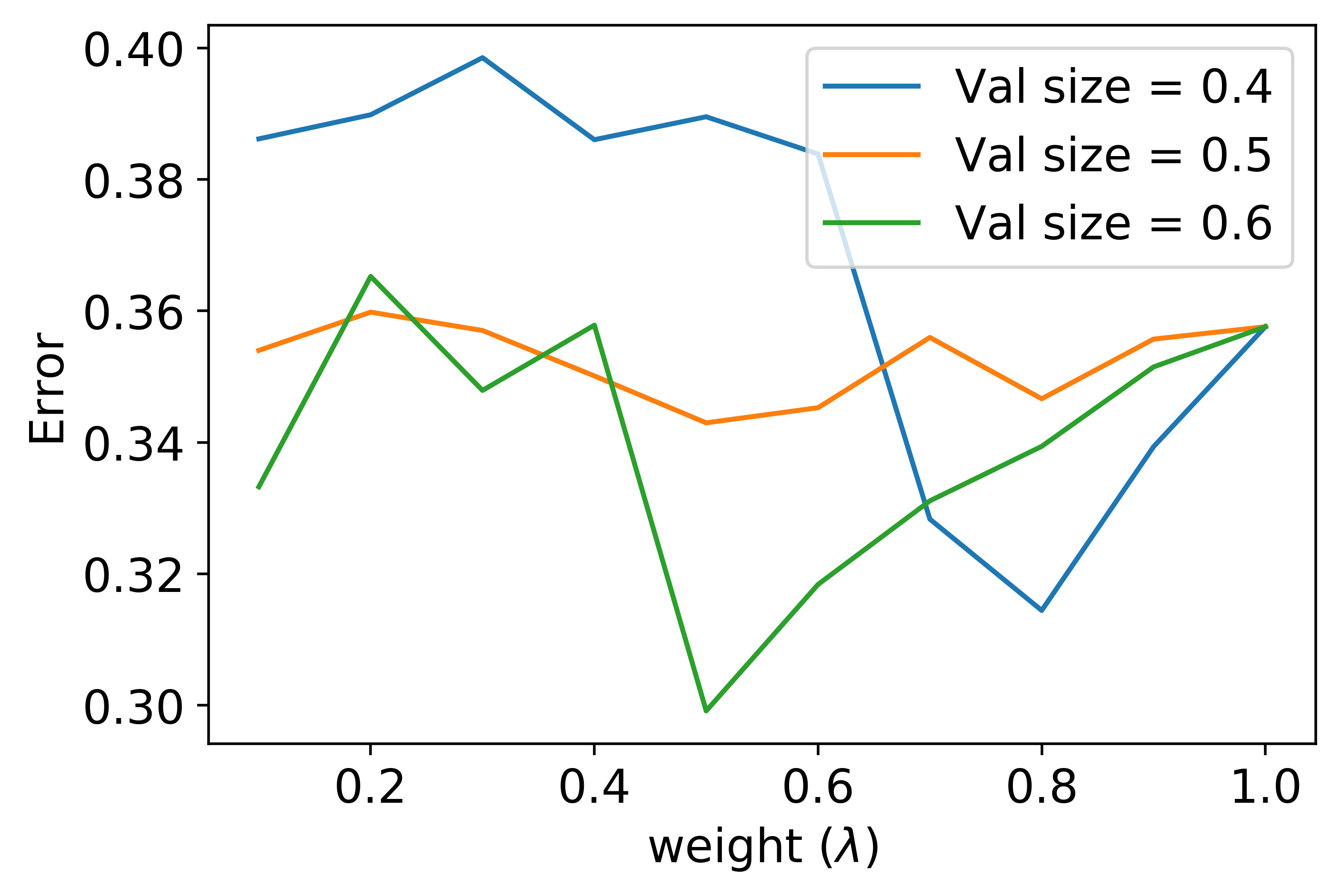
(b) Error across with varying values of $\lambda$.

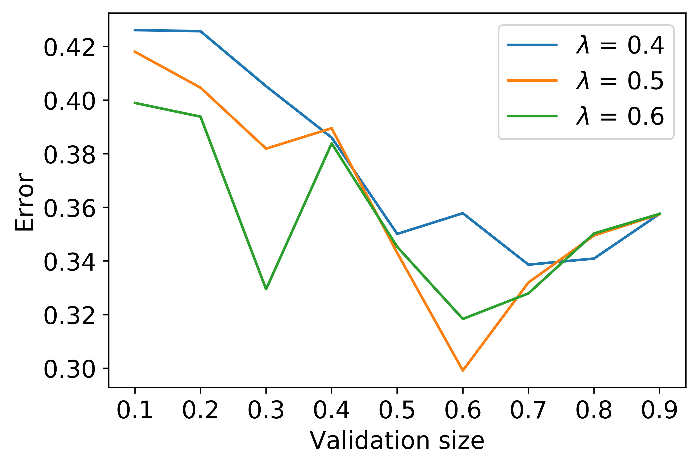
(c) Error across with varying values of validation size.

Figure 3: Plots showing effect of trigger discretization on error rate and hyperparameters using CT-HVP. Fig. 3(a) shows that considering more trigger values leads to lower error, but cannot compete with considering all triggers (0.741 compared to 0.416 in Table 1). Fig. 3(b) and 3(c) show that varying values of $\lambda$ and the validation size effects the error, which suggests need for cross-validation. One way is to use the ACE_error defined in (10).

Table 4: ACIC data error. The results are for non tree methods (e.g. MS), and the unpruned and pruned trees (e.g. CT-L vs CT-LP). Bold results are statistically significant. The table shows that our methods (shaded grey), are significantly better in 18 out of 24 datasets. When our method does not perform better the other methods are not significantly better.

	Data Size = 1000				Data size = 2500				Data size = 5000
Method	32be	5316	d09f	ea8e	6c04	7e4d	95ba	c55e	4e47	9450	a386	f4c2
MS	0.922	0.897	0.685	0.895	0.828	0.823	0.872	0.663	0.914	0.895	0.117	0.200
SD	0.941	0.928	0.711	0.886	0.847	0.838	0.818	0.647	0.944	0.888	0.058	0.360
SM	0.826	0.998	0.400	0.882	0.864	0.953	0.710	0.191	0.864	0.995	0.997	0.223
CT-A	0.927	0.971	0.557	0.933	0.924	0.955	0.752	0.425	0.932	0.999	0.546	0.330
CT-H	0.970	0.998	0.473	0.831	0.905	0.891	0.985	0.244	0.860	0.998	0.855	0.220
CT-L	0.958	0.946	0.319	0.876	0.782	0.929	0.560	0.193	0.907	0.947	0.362	0.168
CT-HL	0.827	0.980	0.189	0.926	0.807	0.894	0.626	0.185	0.802	0.999	0.297	0.016
CT-HV	0.935	0.986	0.296	0.790	0.793	0.887	0.826	0.127	0.909	0.794	0.679	0.108
CT-AP	0.893	0.971	0.484	0.978	0.920	0.954	0.756	0.247	0.930	0.999	0.433	0.290
CT-HP	0.918	0.998	0.341	0.966	0.905	0.961	0.985	0.105	0.924	0.998	0.855	0.149
CT-LP	0.927	0.946	0.319	0.882	0.782	0.924	0.524	0.054	0.918	0.947	0.193	0.135
CT-HLP	0.815	0.980	0.204	0.926	0.807	0.893	0.527	0.185	0.909	0.998	0.002	0.016
CT-HVP	0.926	0.986	0.296	0.889	0.801	0.762	0.826	0.076	0.944	0.883	0.003	0.043
	Data Size = 10000				Data size = 25000				Data size = 50000
Method	0099	0a2a	5cc4	c93b	2e47	4dce	536d	630b	3461	9d8c	a6c1	f2e5
MS	0.649	0.914	0.657	0.398	0.830	0.845	0.754	0.867	0.764	0.918	0.256	0.910
SD	0.698	0.934	0.517	0.367	0.774	0.949	0.737	0.789	0.782	0.916	0.259	0.909
SM	0.293	0.562	0.738	0.609	0.463	0.752	0.959	0.955	0.577	0.895	0.999	0.944
CT-A	0.197	0.872	0.142	0.605	0.350	0.872	0.457	0.961	0.998	0.947	0.996	0.939
CT-H	0.191	0.954	0.176	0.547	0.291	0.835	0.315	0.887	0.977	0.917	0.984	0.973
CT-L	0.189	0.568	0.194	0.461	0.198	0.596	0.076	0.749	0.658	0.894	0.920	0.712
CT-HL	0.251	0.156	0.177	0.657	0.178	0.632	0.153	0.589	0.909	0.998	0.002	0.016
CT-HV	0.092	0.753	0.185	0.349	0.106	0.720	0.060	0.619	0.923	0.888	0.965	0.807
CT-AP	0.157	0.754	0.142	0.466	0.350	0.912	0.448	0.921	0.998	0.947	0.996	0.955
CT-HP	0.084	0.706	0.176	0.366	0.291	0.885	0.108	0.878	0.977	0.915	0.983	0.848
CT-LP	0.077	0.455	0.194	0.176	0.207	0.810	0.076	0.482	0.658	0.894	0.882	0.714
CT-HLP	0.088	0.156	0.177	0.141	0.178	0.857	0.077	0.468	0.884	0.887	0.002	0.016
CT-HVP	0.041	0.753	0.174	0.064	0.106	0.720	0.060	0.451	0.923	0.888	0.965	0.807

We compute the standard deviation of the SMAPE to get statistical significance on the difference between evaluation metrics for different methods. The result is statistically significant if the standard deviations do not intersect.

Evaluation on trigger treatments

Error comparison. Table 1 shows results on the NMES dataset and cloud storage dataset. The adaptive and honest trees were adjusted for building trees on the continuous treatment, using their splitting criterion in tandem with the trigger-based measure. The results of our methods are shaded in grey.

For the NMES dataset, we find that our methods give significantly lower error than the adaptive and honest approaches. Additionally, as seen in Fig. 1, our conclusion is consistent with (?) that prolonged smoking increases medical expenditure. Fig. 1 show the gender and the age when people started smoking are discriminating factors for heterogeneity.

On the cloud storage dataset, we show that our method can get significantly lower error than the adapted CT-A and CT-H methods. Overall, pruning the trees for statistical significance improves the error. In the prepruned trees, our base method, CT-L, performs better. After pruning, CT-HV performs the best. From both datasets, we see that combining the honest penalty with our validation method and metric lowers the error for both trigger-based datasets.

In Fig. 2, we compare two small trees on the cloud storage dataset. We wish to find the trigger age that changes file management decision. In this case, above and below the trigger is considered as old and new, respectively. We show the p-value based on a t-test for the average causal effect (ACE). Positive ACE means that older files are likely to be kept, while negative ACE means likely to be deleted. For example, in the root node for Fig. 2(b), files newer than 1073 days are more likely to be kept. We also see our method can find partitions with ACE that are statistically significant in a low depth. In contrast to the honest trees, statistically significant nodes are found on depth 2. This shows that the adaptation of honest trees to trigger-based treatments is not as effective.

Heterogeneity comparison. Here, we evaluate whether our proposed methods discover more heterogeneous populations by looking at the variance across the discovered leaf effects for each method, as compared to the estimated population effect. Table 2 compares the variance across leaves for the tree-based methods. We observe that the adaptive method finds the highest variance or most heterogeneity. At the same time, the adaptive method has the highest error on both the NMES and Cloud storage datasets, suggesting that the discovered heterogeneity does not have good generalizability. In contrast, our methods consistently find more heterogeneous subgroups compared to the honest method, while having lower error on the datasets. A visual comparison can be made from Fig. 2. We see that the causal effect estimations (ACE) vary much more across leaves in ours compared to CT-H. Visually, this is shown by the shading of nodes, where darker and lighter means more positive and negative ACE. The shading varies much more in CT-L.

Trigger-based selection bias. Next, we test our assumption that the treatment and control populations in each leaf (with treatment value above and below the leaf trigger) have the same underlying distribution. Although trees take care of this to an extent (examples in the same leaf have the same features used on the path), we compare the distance of treatment and control groups. Table 3 compares the average Mahalanobis distance for each tree-based method. For Mahalanobis distance, we compute the distance between each treatment feature vector to the mean of the control group, and each control feature vector the the mean of the treatment, and average over all distances in each leaf. From the table, our proposed CT-HV method has lower population differences at leaves, which means that it deals better with trigger-based selection bias.

Impact of number of triggers. One concern of finding triggers is the increase in complexity of building causal trees. Instead of considering all possible treatment values in the dataset as triggers, we explore the impact of using lower number of possible triggers. Fig. 3(a) shows the number of triggers against the error rate using CT-HV on the NMES dataset. We see that increasing number of considered triggers generally lowers the error. However, we see that even after introducing 100 possible triggers, the error is still significantly higher than when we consider all possible triggers (0.741 compared to an error of 0.416 from Table 1). This shows that there is a significant tradeoff between number of triggers considered and error.

Evaluation on binary treatments

Table 4 shows the error for each ACIC dataset. For each dataset, we compare unpruned (e.g. CT-L) and pruned (e.g. CT-LP) tree results separately. We bold statistically significant results. Our methods are shaded in grey.

Across all the datasets, we see that our proposed methods achieve lower error compared to the previous tree-based methods. For those datasets where our method is not significantly better, the other methods do not have significantly lower error. Our variants (CT-HL and CT-HV) generally have lower error than our base method. Careful validation should be done to choose the best method.

We notice that some of the datasets have very large error error ($>0.9$). A likely reason is that the range of the response variable varies wildly in some cases. For example, in dataset 9450, the range of response is about 429. When building the tree, large values affect the ACE at each node.

Hyperparameter tuning

Since we introduce two hyperparameters in our methods, namely the weight $\lambda$ for controlling validation penalty, and the validation split size, we explore varying these values.

Fig. 3(b) shows the error rate for varying values of $\lambda$ across different validation sizes. From this plot, we see that with sizes of the validation set, the lowest error changes with different values of $\lambda$. We notice that a larger $\lambda$ is needed for smaller validation, while a smaller $\lambda$ is needed for larger validation. Also, the error seems to be more stable when the validation is the same size as the training set.

Fig. 3(c) shows the error rate for varying validation sizes, with $\lambda$ fixed. We can infer that having a validation size close to the size of the training size is a good choice for lower error. From both figures, we conclude using a method for learning these parameters is important. Cross-validation can be used to tune these parameters (e.g. using (10)).

Conclusion

In this paper, we define the problem of trigger-based heterogeneous treatment effect estimation. To do this, we propose novel splitting criteria for building causal trees and incorporate validation data to improve generalizability. We introduce the use of a validation set for HTE estimation for learning optimal partitioning, by introducing a loss function that penalizes partitions whose effects do not generalize. We showed our method can get better coverage on average causal effect on unseen test data when identifying triggers. Our experimental results show our method performs better than previous causal tree methods for binary treatment estimation. Important future directions include outlier detection for decreasing sample variance, developing methods for different distribution assumptions, such as non-i.i.d data, and incorporating matching methods into HTE estimation.

References

- [Almardini et al. 2015] Almardini, M.; Hajja, A.; Raś, Z. W.; Clover, L.; Olaleye, D.; Park, Y.; Paulson, J.; and Xiao, Y. 2015. Reduction of readmissions to hospitals based on actionable knowledge discovery and personalization. In Beyond Databases, Architectures and Structures. Advanced Technologies for Data Mining and Knowledge Discovery. Springer. 39–55.
- [Ascarza 2018] Ascarza, E. 2018. Retention futility: Targeting high-risk customers might be ineffective. Journal of Marketing Research 55(1):80–98.
- [Athey and Imbens 2015] Athey, S., and Imbens, G. W. 2015. Machine learning methods for estimating heterogeneous causal effects. stat 1050(5).
- [Athey and Imbens 2016] Athey, S., and Imbens, G. 2016. Recursive partitioning for heterogeneous causal effects. Proceedings of the National Academy of Sciences.
- [Athey, Tibshirani, and Wager 2016] Athey, S.; Tibshirani, J.; and Wager, S. 2016. Generalized random forests. arXiv preprint arXiv:1610.01271.
- [Breiman 2017] Breiman, L. 2017. Classification and regression trees. Routledge.
- [Foster, Taylor, and Ruberg 2011] Foster, J. C.; Taylor, J. M.; and Ruberg, S. J. 2011. Subgroup identification from randomized clinical trial data. Statistics in Medicine 30(24):2867–2880.
- [Green and Kern 2012] Green, D. P., and Kern, H. L. 2012. Modeling heterogeneous treatment effects in survey experiments with bayesian additive regression trees. Public Opinion Quarterly 76(3):491–511.
- [Grimmer, Messing, and Westwood 2017] Grimmer, J.; Messing, S.; and Westwood, S. J. 2017. Estimating heterogeneous treatment effects and the effects of heterogeneous treatments with ensemble methods. Political Analysis 25(4):413–434.
- [Imai and Ratkovic 2013] Imai, K., and Ratkovic, M. 2013. Estimating treatment effect heterogeneity in randomized program evaluation. The Annals of Applied Statistics 7(1):443–470.
- [Imai and Van Dyk 2004] Imai, K., and Van Dyk, D. A. 2004. Causal inference with general treatment regimes: Generalizing the propensity score. Journal of the American Statistical Association 99(467):854–866.
- [Johnson et al. 2003] Johnson, E.; Dominici, F.; Griswold, M.; and Zeger, S. L. 2003. Disease cases and their medical costs attributable to smoking: an analysis of the national medical expenditure survey. Journal of Econometrics 112(1):135–151.
- [Kallus and Zhou 2018] Kallus, N., and Zhou, A. 2018. Policy evaluation and optimization with continuous treatments. arXiv preprint arXiv:1802.06037.
- [Kallus 2017] Kallus, N. 2017. Recursive partitioning for personalization using observational data. In International Conference on Machine Learning, 1789–1798.
- [Khan et al. 2018] Khan, M. T.; Hyun, M.; Kanich, C.; and Ur, B. 2018. Forgotten but not gone: Identifying the need for longitudinal data management in cloud storage. In Proceedings of the 2018 CHI Conference on Human Factors in Computing Systems, 543. ACM.
- [Laber and Zhao 2015] Laber, E., and Zhao, Y. 2015. Tree-based methods for individualized treatment regimes. Biometrika 102(3):501–514.
- [Lakkaraju and Rudin 2017] Lakkaraju, H., and Rudin, C. 2017. Learning cost-effective and interpretable treatment regimes. In Artificial Intelligence and Statistics, 166–175.
- [Li et al. 2010] Li, L.; Chu, W.; Langford, J.; and Schapire, R. E. 2010. A contextual-bandit approach to personalized news article recommendation. In Proceedings of the 19th international conference on World wide web, 661–670. ACM.
- [Rosenbaum and Rubin 1983] Rosenbaum, P. R., and Rubin, D. B. 1983. The central role of the propensity score in observational studies for causal effects. Biometrika 70(1):41–55.
- [Rubin 1974] Rubin, D. B. 1974. Estimating causal effects of treatments in randomized and nonrandomized studies. Journal of Educational Psychology 66(5):688.
- [Rubin 1978] Rubin, D. B. 1978. Bayesian inference for causal effects: The role of randomization. The Annals of Statistics 34–58.
- [Spratt et al. 2013] Spratt, D. E.; Pei, X.; Yamada, J.; Kollmeier, M. A.; Cox, B.; and Zelefsky, M. J. 2013. Long-term survival and toxicity in patients treated with high-dose intensity modulated radiation therapy for localized prostate cancer. International Journal of Radiation Oncology• Biology• Physics 85(3):686–692.
- [Su et al. 2009] Su, X.; Tsai, C.-L.; Wang, H.; Nickerson, D. M.; and Li, B. 2009. Subgroup analysis via recursive partitioning. Journal of Machine Learning Research 10(Feb):141–158.
- [Tian et al. 2014] Tian, L.; Alizadeh, A. A.; Gentles, A. J.; and Tibshirani, R. 2014. A simple method for estimating interactions between a treatment and a large number of covariates. Journal of the American Statistical Association 109(508):1517–1532.
- [Wager and Athey 2017] Wager, S., and Athey, S. 2017. Estimation and inference of heterogeneous treatment effects using random forests. Journal of the American Statistical Association.
- [Wang et al. 2014] Wang, X.; Ouyang, Y.; Liu, J.; Zhu, M.; Zhao, G.; Bao, W.; and Hu, F. B. 2014. Fruit and vegetable consumption and mortality from all causes, cardiovascular disease, and cancer: systematic review and dose-response meta-analysis of prospective cohort studies. Bmj 349:g4490.
- [Xie, Brand, and Jann 2012] Xie, Y.; Brand, J. E.; and Jann, B. 2012. Estimating heterogeneous treatment effects with observational data. Sociological methodology 42(1):314–347.
- [Xie, Chen, and Shi 2018] Xie, Y.; Chen, N.; and Shi, X. 2018. False discovery rate controlled heterogeneous treatment effect detection for online controlled experiments. In Proceedings of the 24th ACM SIGKDD International Conference on Knowledge Discovery and Data Mining, 876–886. ACM.
- [Xu et al. 2015] Xu, Y.; Yu, M.; Zhao, Y.-Q.; Li, Q.; Wang, S.; and Shao, J. 2015. Regularized outcome weighted subgroup identification for differential treatment effects. Biometrics 71(3):645–653.
- [Zeileis, Hothorn, and Hornik 2008] Zeileis, A.; Hothorn, T.; and Hornik, K. 2008. Model-based recursive partitioning. Journal of Computational and Graphical Statistics 17(2):492–514.