An open and parallel multiresolution framework using block-based adaptive grids

Abstract

A numerical approach for solving evolutionary partial differential equations in two and three space dimensions on block-based adaptive grids is presented. The numerical discretization is based on high-order, central finite-differences and explicit time integration. Grid refinement and coarsening are triggered by multiresolution analysis, i.e. thresholding of wavelet coefficients, which allow controlling the precision of the adaptive approximation of the solution with respect to uniform grid computations. The implementation of the scheme is fully parallel using MPI with a hybrid data structure. Load balancing relies on space filling curves techniques. Validation tests for 2D advection equations allow to assess the precision and performance of the developed code. Computations of the compressible Navier-Stokes equations for a temporally developing 2D mixing layer illustrate the properties of the code for nonlinear multi-scale problems. The code is open source.

1 Introduction

For many applications in computational fluid dynamics, adaptive grids are more advantageous than uniform grids, because computational efforts are put at locations required by the solution. Since small-scale flow structures may travel, emerge and disappear, the required local resolution is time-dependent. Therefore dynamic gridding, which tracks the evolution of the solution, is more efficient than static grids. However, suitable grid adaptation techniques are necessary to dynamically track the solution. These techniques can increase the computational cost, therefore their efficiency is problem dependent and related to the sparsity of the adaptive grid.

Examples where adaptivity is beneficial are reactive flows with localized flame fronts, detonations and shock waves [1, 23], coherent structures in turbulence [24] and flapping insect flight [12]. For the latter the time-varying geometry generates localized turbulent flow structures. These applications motivate and trigger the development of a novel multiresolution framework, which can be used for many mixed parabolic/hyperbolic partial differential equations (PDE).

The idea of adaptivity is to refine the grid where required and to coarsen it where possible, while controlling the precision of the solution.

Such approaches have a long tradition and can be traced back to the late seventies [5]. Adaptive mesh refinement and multiresolution concepts developed by Berger et al. [2] and Harten [14, 15], respectively, are meanwhile widely used for large scale computations (e.g. [20, 18, 11]).

Berger suggested a flexible refinement strategy by overlaying different grids of various orientation and size, in the following referred to as adaptive mesh refinement (AMR). Harten instead discusses a mathematical more rigorous wavelet based method, termed multiresolution (MR). For AMR methods, the decision where to adapt the grid is based on error indicators, such as gradients of the solution or derived quantities. In contrast in MR, the multiresolution transform allows efficient compression of data fields by thresholding detail coefficients. This multiresolution transform is equivalent to biorthogonal wavelets, see e.g. [15]. An important feature of MR is the reliable error estimator of the solution on the adaptive grid, as the error introduced by removing grid points can be directly controlled.

In wavelet-based approaches the governing equations are discretized, either by using wavelets in a Galerkin or collocation approach [24], or using a classical discretization, e.g. finite volumes or differences, where the grid is adapted locally using MR analysis [4, 11].

MR methods typically keep only the information which is dictated by a threshold criterion, which is refereed to as sparse point representation (SPR), introduced in [16]. AMR methods often utilize blocks and refine complete areas, by which the maximal sparsity is typically abandoned in favor of a simpler code structure. An example of this approach is the AMROC code [8], where blocks of arbitrary size and shape are refined. A detailed comparison of MR with AMR techniques has been carried out in [9].

For practical applications both the data compression and the speed-up of the calculation are crucial. The latter is reduced by the computational overhead to handle the adaptive grid and corresponding datastructures. This effort differs substantially between different approaches [19]. It can be reduced by refining complete blocks, thereby reducing the elements to manage, and by exploiting simple grid structures.

A MR method using a quad- or octtree representation to simplify the grid structure is reported, e.g., in [10, 11] and has later also been used in [22].

For detailed reviews on the subject of multiresolution methods we refer the reader to [7, 24, 18, 24, 11]. Implementation issues have been discussed in [6].

Our aim is to provide a multiresolution framework, which can be easily adapted to different two- and three-dimensional simulations encountered in CFD, and which can be efficiently used on fully parallel machines.

To this end the chosen framework is block based, with nested blocks on quad- or octree grids. The individual blocks define structured grids with a fixed number of points. Refinement and coarsening are controlled by a threshold criterion applied to the wavelet coefficients. The software, termed “wavelet adaptive block-based solver for interactions with turbulence” (WABBIT), is open-source and freely available in order to maximize its utility for the scientific community and for reproducible science.

The purpose of this paper is to introduce the code, present its main features and explain structural and implementation details. It is organized as follows. In section 2 we give an overview of implementation and structure details. Numerics will only be shortly described, but special issues of our data structure, interpolation, and the MPI coding will be explained in detail. Section 3 considers a classical validation test case, including a discussion on the adaptivity and convergence order of WABBIT. In section 4 we present computations for a temporally developing double shear layer, governed by the compressible Navier-Stokes equations. Section 5 draws conclusions and gives perspectives for future work.

2 Code structure

In this section we present a detailed description of the data and code structure. One of the main concepts in WABBIT is the encapsulation and separation of the set of PDE from the rest of the code, thus the PDE implementation is not significantly different from that in a single domain code and can easily be exchanged. The code solves evolutionary PDE of the type $\partial_{t}\phi=N(\phi)$. The spatial part $N(\phi)$ is referred to as right hand side in this report. A primary directive for the code is its “explicit simplicity”, which means avoiding complex programming structures to improve maintainability. WABBIT is written in Fortran 95 and aims at reaching high performance on massively parallel machines with distributed memory architecture. We use the MPI library to parallelize all subroutines, while parallel I/O is handled through the HDF5 library.

2.1 Multiresolution algorithm

The main structure of the code is defined by the multiresolution algorithm. After the initialization phase, the general process to advance the numerical solution $\varphi\left(t^{n},x\right)$ on the grid $\mathcal{G}^{n}$ to the new time level $t^{n+1}$ can be outlined as follows.

1. Refinement. We assume that the grid $\mathcal{G}^{n}$ is sufficient to adequately represent the solution $\varphi\left(t^{n},x\right)$, but we cannot suppose this will be true at the new time level. Non-linearities may create scales that cannot be resolved on $\mathcal{G}^{n}$, and transport can advect existing fine structures. Therefore, we have to extend $\mathcal{G}^{n}$ to $\mathcal{\widetilde{G}}^{n}$ by adding a “safety zone” [24] to ensure that the new solution $\varphi\left(t^{n+1},x\right)$ can be represented on $\mathcal{\widetilde{G}}^{n}$. To this end, all blocks are refined by one level, which ensures that quadratic non-linearities cannot produce unresolved scales.

2. Evolution. On the new grid $\mathcal{\widetilde{G}}^{n}$, we first synchronize the layer of ghost nodes (section 2.5) and then solve the PDE using finite differences and explicit time-marching methods.

3. Coarsening. We now have the new solution $\varphi(t^{n+1},x)$ on the grid $\mathcal{\widetilde{G}}^{n}$. The grid $\mathcal{\widetilde{G}}^{n}$ is a worst-case scenario and guarantees resolving $\varphi(t^{n+1},x)$ using a priori knowledge on the non-linearity. It can now be coarsened to obtain the new grid $\mathcal{G}^{n+1}$, removing, in part, blocks created during the refinement stage. Section 2.3 explains this process in more detail.

4. Load balancing. The remaining blocks are, if necessary, redistributed among MPI processes using a space-filling curve [25], such that all processes compute approximately the same number of blocks. The space-filling curve allows preservation of locality and reduces interprocessor communication cost.

2.2 Block- and Grid Definition

Block definition.

The decomposition of the computational domain builds on blocks as smallest elements, as used for example in [10]. The approach thus builds on a hybrid datastructure, combining the advantages of structured and unstructured data types. The structured blocks have a high CPU caching efficiency. Using blocks instead of single points reduces neighbor search operations. A drawback of the block based approach is the reduced compression rate.

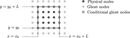
Figure 1: Definition of a block with $B_{s}=5$ and $n_{g}=1$.

A block is illustrated in Fig. 1. Its definition (in 2D) is

$$\mathcal{B}^{\ell}=\left\{\underline{x}=\underline{x}_{0}+\left(i\cdot\Delta x^{\ell},j\cdot\Delta x^{\ell}\right)^{T},\;0\leq i,j\leq B_{s}\right\}$$

where $\underline{x}_{0}$ is the blocks origin, $\Delta x^{\ell}=2^{-\ell}L/(B_{s}-1)$ is the lattice spacing at level $\ell$, and $L$ the size of the entire computational domain. The mesh level encodes the refinement from 1 as coarsest to the user defined value $J_{\mathrm{max}}$ as finest. Blocks have $B_{s}$ points in each direction, where $B_{s}$ is odd, which is a requirement of the grid definition we use. We add a layer of $n_{g}$ ghost points that are synchronized with neighboring blocks (see section 2.5). The first layer of physical points is called conditional ghost nodes, and they are defined as follows:

1. If the adjacent block is on the same level, then the conditional ghost nodes are part of both blocks and thus redundant in memory; their values are identical.

2. If the levels differ, the conditional ghost nodes belong to the block on the finer level, i.e., their values will be overwritten by those on the finer block.

Grid definition.

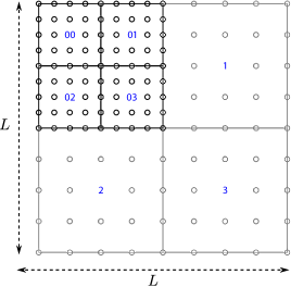
Figure 2: Example grid with $N_{b}=7$ blocks. Three blocks on mesh level 1 (gray) and four on level 2 (black), together with their treecodes. Note that the mesh level is equal to the length of the treecode. Points at the coarse/fine interface belong to finer blocks.

A complete grid consisting of $N_{b}=7$ blocks is shown in Fig. 2. We force the grid to be graded, i.e., we limit the maximum level difference between two blocks to one. Blocks are addressed by a quadtree-code (or an octtree in 3D), as introduced in [13], and also shown in Fig. 2. Each digit of the treecode represents one mesh level, thus its length indicates the level $\ell$ of the block. If a block is coarsened, the last digit is removed, while for refinement refinement, one digit is added. The function of the treecode is to allow quick neighbor search, which is essential for high performance. For a given treecode the adjacent treecodes can easily be calculated [13]. A list of the treecodes of all existing blocks allows us to find the data of the neighboring block, see section 2.4. To ensure unique and invertible neighbor relations, we define them not only containing the direction but also encode if a block covers only part a border. This situation occurs if two neighboring blocks differ in level. We also account for diagonal neighborhoods. In two space dimensions 16 different relations defined (74 in 3D). This simplifies the ghost nodes synchronization step, since all required information, the neighbor location and interpolation operation are available.

Right hand side evaluation.

The PDE subroutine purely acts on single blocks. Therefore efficient, single block finite difference schemes can be used allowing to combine existing codes with the WABBIT framework. Adapting the block size to the CPU cache offers near optimal performance on modern hardware. The size of the ghost node layer can be chosen freely, to match numerical schemes with different stencil sizes.

2.3 Refinement / coarsening of blocks.

If a block is flagged for refinement by some criteria (see blow) this refinement is executed as illustrated in Fig. 3. The block, with synchronized ghost points, is first uniformly upsampled by midpoint insertion, i.e., missing values on the grid

$$\mathcal{\widetilde{B}}^{\ell}=\left\{\underline{x}=\underline{x}_{0}+\left(i\cdot\Delta x^{\ell}/2,j\cdot\Delta x^{\ell}/2\right)^{T},\quad-2n_{g}\leq i,j\leq 2B_{s}-1+2n_{g}\right\}$$

are interpolated (gray points in Fig. 3 center). In other words, a prediction operator $\mathcal{P}_{\ell\rightarrow\ell+1}$ is applied [14]. The data is then distributed to four new blocks $\mathcal{B}_{i}^{\ell+1}$, where one digit is added to the treecode, which are created on the MPI process holding the initial (“mother”) block. The blocks are nested, i.e. all nodes of a coarser block also exist in the finer one. The reverse process is coarsening, where four sister blocks on the same level are merged into one coarser block by applying the restriction operator $\mathcal{R}_{\ell\rightarrow\ell-1}$, which simply removes every second point. For coarsening, no ghost node synchronization is required, but all four blocks need to be gathered on one MPI rank.

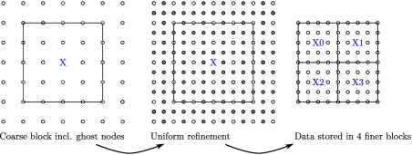
Figure 3: Process of refining block with treecode X. First, the block is upsampled, including the ghost nodes layer. Then, four new blocks are created, where one digit is added to the treecode.

The refinement operator uses central interpolation schemes. Using one-sided schemes close to the boundary would not require ghost points and would thus reduce the number of communications. They yield errors only of the order of the threshold $\varepsilon$. However, the small, but non-smooth structures of these errors force very fine meshes, which can increase the number of blocks. This fill-up can lead to prohibitively expensive calculations.

Computation of detail coefficients.

The decision whether a block can be coarsened or not is made by calculating its detail coefficients [24]. The are computed by first applying the restriction operator, followed by the prediction operator. After this round trip of restriction and prediction, the original resolution is recovered, but the values of the data differ slightly. The difference

$$\mathcal{D}=\{d(\underline{x})\}=\mathcal{B}^{\ell}-\mathcal{P}_{\ell-1\rightarrow\ell}(\mathcal{R}_{\ell\rightarrow\ell-1}(\mathcal{B}^{\ell}))$$

is called details. If details are small, the field is smooth on the current grid level. Therefore, the details act as indicator for a possible coarsening [14]. Non-zero details are obtained at odd indices only (gray points in Fig. 3, center) because of the nested grid definition and the fact that restriction and prediction do not change these values. The refinement flag for a block is then

$$r=\begin{cases}-1&\text{if }\left\|d(\underline{x})\right\|_{\infty}<\varepsilon\\ \phantom{-}0&\text{otherwise}\end{cases}$$

where -1 indicates coarsening and 0 no change. In other words, the largest detail sets the status of the block. Note, that WABBIT technically provides the possibility to flag -1 for coarsening, 0 for unaltered and +1 for refinement, it can hence be used with arbitrary indicators. Since a block cannot be coarsened if its sister blocks on the same root do not share the +1 refinement status, WABBIT assigns the -2 status for blocks that can indeed be coarsened, after checking for completeness and gradedness.

2.4 Data structure

The data are split into two kinds of data, first, the field data (the flow fields) required to calculate the PDE and, second, the data to administer the block decomposition and the parallel distribution.

Data which are held only on one specific MPI process are called heavy data. This is the (typically large) field data and the neighbor relations for the blocks held by the MPI process. The field data (hvy_block) is a five dimensional array where the first three indices describe the note within a block (3D notation is always used in the code), the fourth index the index of the physical variables and the last one the block index identifying it within the MPI process.

The light data (lgt_block) are data which are kept synchronous between all processes. They describe the global topology of the adapted grid and change during the computation. The light data consist of the block treecode, the block mesh level and the refinement flag. Additionally, we encode the MPI process rank $i_{\mathrm{process}}$ and the block index on this process $j_{\mathrm{block}}$ by the position $I$ of the data within the light data array, $I=(i_{\mathrm{process}}-1)\cdot N_{\mathrm{max}}+j_{\mathrm{block}}$, where $N_{\mathrm{max}}$ is the maximal number of blocks per process. The light data enable each process to determine the process holding neighboring blocks, by looking for the index $I$ corresponding to the adjacent treecode. The number of blocks required during the computation is unknown before running the simulation. To avoid time consuming memory allocation, $N_{\mathrm{max}}$ is typically determined by the available memory. This sets the index range of the last index of the heavy data and determines the size of the light data. Hence, many blocks are typically unused; they are marked by setting the treecode in the light data list to -1. To accelerate the search within the light data, we keep a second list of indices holding active entries.

2.5 Parallel implementation

Data synchronization.

For parallel computing, an efficient data synchronization strategy is essential for good performance. There are two different tasks in WABBIT, namely light and heavy data synchronisation. Light data synchronization is an MPI all-to-all operation, where we communicate active entries of the light data only. Heavy data synchronization, i.e. filling the ghost nodes layer of each block, is much more complicated. We have to balance a small number of MPI calls and a small amount of communicated data, and additionally we have to ensure that no idle time occurs due to blocking of a process by a communication in which this process is not involved. To this end, we use MPI point-to-point communication, namely non-blocking non-buffered send/receive calls. To reduce the number of communications, the ghost point data of all blocks belonging to one process are gathered and send as one chunk. After the MPI communications, all processes store received data in the ghost point layers.

The conditional ghost nodes require special attention during the synchronization. To ensure that neighboring blocks always have the same values at these nodes, the redundant nodes are sent, when required, to the neighboring process. Blocks on higher mesh levels (finer grids) always overwrite the redundant nodes to neighbors on lower mesh level (coarser grid). It is assumed that two blocks on the same mesh level never differ at a redundant node, because any numerical scheme should always produce the same values.

Load balancing.

The external neighborhood consists of ghost nodes, which may be located on other processes and therefore have to be sent/received in the heavy data synchronization step. Internal ghost nodes can simply be copied within the process memory, which is much faster than MPI communication. It is, thus, desired to reduce inter-process neighborhood. We use space filling curves [25] to redistribute the blocks among the processes for their good localization. The computation of the space filling curve is simple, because we can use the treecode to calculate the index on the curve.

3 Advection test case

As a validation case, we now consider a benchmarking problem for the 2D advection equation, $\partial_{t}\varphi+u\cdot\nabla\varphi=0$, where $\varphi(x,y,t)$ is a scalar and $0\leq x,y<1$. The spatially-periodic setup considers time-periodic mixing of a Gaussian blob,

$$\varphi(x,y,0)=e^{-\left((x-c)^{2}+(y-d)^{2}\right)/\beta}$$

where $c=0.5$, $d=0.75$ and $\beta=0.01$. The time-dependent velocity field is given by

$$u(x,y,t)=\cos\left(\dfrac{\pi t}{t_{a}}\right)\left(\begin{array}[]{cc}\sin^{2}(\pi x)\sin(2\pi y)\\ \sin^{2}(\pi y)(-\sin(2\pi x))\end{array}\right)$$ (1)

and swirls the initial distribution, but reverses to the initial state at $t=t_{a}$. The swirling motion produces increasingly fine structures until $t=t_{a}/2$, where $t_{a}$ controls also the size of structures. The larger $t_{a}$, the more challenging is the test.

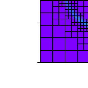
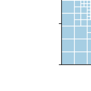
Figure 4: Shown is a pseudocolor-plot of $\varphi$ at times $t=0$, $t=t_{a}/2=2.5$ and the distribution of the blocks among the MPI processes by different colors at $t=2.5$ (from left to right). Each block covers $33\times 33$ points.

Spatial derivatives are discretized with a 4th-order, central finite-difference scheme and we use a 4th-order Runge–Kutta time integration. Interpolation for the refinement operator is also 4th order. We compute the solution for $t_{a}=5$, for various maximal mesh levels $J_{\mathrm{max}}$. The computational domain is a unit square and we use a block size of $33\times 33$.

Figure 4 illustrates $\varphi$ at the initial time, $t=0$, and the instant of maximal distortion at $t=2.5=t_{a}/2$. At $t=2.5$ the grid is strongly refined in regions of fine structures, while the remaining part of the domain features a coarser resolution, e.g., in the center of the domain. Further the distribution among the MPI processes is shown by different colors, revealing the locality of the space filling curve.

In the following we compare soloutions with the finest strutures at $t=t_{a}/2$ with a reference solution, to investigate the quality and performance. The reference solution is obtained with a pseudo-spectral code on a sufficiently fine mesh to have a negligible error compared with the current results.

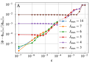
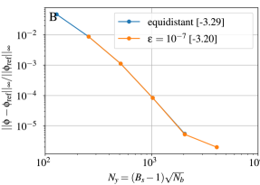
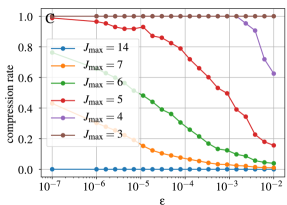
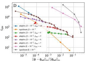
Figure 5: Swirl test for varying $J_{\mathrm{max}}$ and $\varepsilon$. A: For different maximal refinement levels a saturation of the error is seen at different values of $\varepsilon$, showing the cross over form threshold- to discretization-error. B: Error decay for fixed $\varepsilon=10^{-7}$ and varying $J_{\mathrm{max}}$ (i.e. the rightmost data points in A) as a function of the number of points in one direction. The adaptive computation preserves roughly the 4^th order accuracy of the discretization scheme. C: Compression rate defined as block of the adaptive mesh compared with a equidistant mesh constantly on the same $J_{\mathrm{max}}$. D: The CPU time as a function of discretization error for two different initial conditions. For the broad pulse ($\beta=10^{-2}$) the adaptive solution is faster for an appropriate choice of $J_{\mathrm{max}}(\varepsilon)$ for the finer pules ( $\beta=10^{-2}$) it is faster even for a constant $J_{\mathrm{max}}=\infty$ for relevant errors.

Fig. 5A illustrates the relative error, computed as the $\infty$-norm of the difference $\varphi-\varphi_{\mathrm{ex}}$, normalized by $||\varphi_{\mathrm{ex}}||_{\infty}$. All quantities are evaluated on the terminal grid. A linear least squares fit exhibits convergence orders close to one for the large maximal refinements. In this case the error decays, as expected, linearly in $\varepsilon$. For smaller $J_{\mathrm{max}}$ we find a saturation of the error, which is determined by the highest allowed resolution. This different levels are plotted in Fig. 5B, where a convergence order close to four, as expected by the space and time discretization is found. Thus, the points where the saturation sets in are turnover points form an threshold to and cut-off dominated error. For the sake of efficiency one aims to be close to this turnover point where both errors are of similar size. In Fig. 5C the compression rate, i.e. the number of blocks relative to an equidistant grid constantly on the level of the same $J_{\mathrm{max}}$ is depicted. As expected the compression becomes close to one for small $\varepsilon$. In Fig. 5D the error is shown as a function of the computational time for two initial conditions, the broad pulse with $\beta=10^{-2}$ and a narrower one with $\beta=10^{-4}$. For the broad pulse ($\beta=10^{-2}$) the curves for different $J_{\mathrm{max}}$ are below the equidistant curve only for carefully chosen values of $\varepsilon$. This is explained by the wide area of refinement at the final time, see Fig. 4. Here a multi-resolution method cannot win much. Even for $J_{\mathrm{max}}=14$, which in practice means deactivating the level restriction, a similar scaling as for the equidistant grid is found with a factor approaching about four. Thus, even without tuning $J_{\mathrm{max}}(\varepsilon)$ accordingly, and given the low cost of the right hand side, the computational complexity of the adaptive code scales reasonably compared to the equidistant solution. For a finer initial condition ($\beta=10^{-4}$), even without the level restriction ( $J_{\mathrm{max}}=\infty$), the adaptive code produces better run-times for practical relevant errors.

4 Navier-Stokes test case

In this section we present the results of a second test case, governed by the ideal-gas, constant heat capacity compressible Navier-Stokes equations in the skew-symmetric formulation [21]. A double shear-layer in a periodic domain is perturbed so that the growing instabilities end up with small scale structures, similar to [17]. The size of the computational domain is $L=L_{x}=L_{y}=8$ and the shear layer is initially located at $\frac{L}{2}\pm 0.25$. The density and $y$-velocity is $\rho_{1}=2$ and $v_{1}=1$ between the shear layers and $\rho_{0}=1$ and $v_{0}=-1$ otherwise. At the jumps it is smoothed by $\tanh((y-y_{\mathrm{jump}})/\lambda_{w})$ with a width $\lambda_{w}=L/240$. The the initial pressure is uniformly $p=2.5$. The $x$-velocity is disturbed to induce the instability in a controlled manner by $u=\lambda\sin(2\pi(y-L/2))$ with $\lambda=0.1$. The dynamic viscosity is given by $\mu=10^{-6}$. The adiabatic index is $\gamma=1.4$ and the Prandtl number is $Pr=0.71$ and the specific gas constant $R_{\mathrm{s}}=287.05$.

We discretize spatial derivatives with standard 4th-order central differencing scheme, use the standard 4th-order Runge-Kutta time integration and for interpolation a 4th-order scheme. We use global time stepping so that the time step is (usually) determined by the time step at the highest mesh level. We apply a shock capturing filter as described in [3] with a threshold value of $r_{\mathrm{th}}=10^{-5}$ in every time step. Filtering, as any procedure to suppress high wave numbers (e.g. flux limiter, slope limiter or numerical damping), interacts with the MR. No special modification beyond the previously described [21] smoothed detector, was necessary for the use with the multi resolution framework. The investigation of the interplay between filtering and MR is left for future work.

Figure 6: Double shear layer, plot of density $\rho$ and the absolute value of the vorticity $|\omega|$ at time $t=4$ on an adaptive grid with threshold value $\varepsilon=1$e-$3$, maximum mesh level $J_{\mathrm{max}}=8$.

In Fig. 6 the density field for adaptive computations with a threshold $\varepsilon=10^{-3}$ at $t=4$ is shown. In both density and vorticity field one can observe small scale structures created by the shear layer instability. The size and form of the structures are in agreement with [17].

In the right of Fig. 7 the compression rate of the shear layer is plotted over time. We start with a low number of blocks (i.e. low values of the compression rate), the grid fills up to the maximal refinement with simulation time. This is explained by short wavelength acoustic waves emitted by the shear layer. Depending on the investigation target a modified threshold criterion, e.g., applying it only to certain variables might be beneficial. For this the error estimation must be reviewed and it is left for future work.

In Fig. 7 we show the kinetic energy spectra for these computations compared to the result for a fixed grid. To calculate the energy spectra we refine the mesh after the computation to a fixed mesh level, if needed. They agree well on the resolved scales. For the higher maximum mesh level $J_{\mathrm{max}}$ we observe a better resolution of the small scale structures. Summarized, if we compare adaptive and fixed mesh computation, we can observe a good resolution of the small scales within the double shear layer.

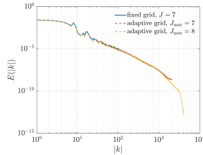
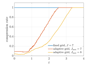
Figure 7: Left: Energy spectrum of the double shear layer. The computations were performed on a fixed grid with mesh level $J=7$, and on adaptive grids with threshold value $\varepsilon=10^{-3}$, maximum mesh level $J_{\mathrm{max}}=7$, $J_{\mathrm{max}}=8$, $t=4$. Right: The compression rate. After high initial copressions the grid fills up due to high wavenumber acoustic waves.

Fig. 8 shows the strong scaling behavior for the adaptive double shear layer computation with $J_{\mathrm{max}}$ = 7. We observe a scaling which is predicted by Amdahl’s law with a parallel fraction of 0.99. The observed strong scaling is reasonable and we anticipate that code optimization will yield further improvements.

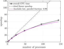
Figure 8: From the strong scaling a parallel fraction of 99% can be estimated.

5 Conclusions and Perspectives

The novel framework WABBIT with its main structures and concepts has been described. WABBIT uses a multiresolution algorithm to adapt the mesh to capture small localized structures. Within the framework different equation sets can be used.

We showed that the error due to the thresholding is controlled and scales nearly linear. In the Gaussian pulse test case we found that the maximum number of blocks is reached at the largest deformation of the pulse and after that the mesh is coarsen with several orders of magnitude. We observed that the fill-up was strongly reduced by using a symmetric interpolation stencil, which will be investigated in future work.

In the second test case we showed an application of the compressible Navier-Stokes equations. Here we saw a good resolution of small scale structures and observed the impact of discarding wavelet coefficient on the physics of the shear layer. In our simulations we observe a reasonable strong scaling. Scaling will be assessed in more detail when foreseen improvements are implemented.

In the near future we will extend the physical situation by using reactive Navier-Stokes equations to simulate turbulent flames. Validation for 3D problems and further improvement of the performance is currently worked on. For this an additional parallelization with openMP is in preparation, which should reduce the communication effort further in typical cluster architecture. Further a generic boundary handling within the frame work and an interface to connect other MPI programs is under way.

Acknowledgments.

MS and JR thankfully acknowledge funding by the Deutsche Forschungsgemeinschaft (DFG) (grant SFB-1029, project A4). TE and KS acknowledge financial support from the Agence nationale de la recherche (ANR Grant 15-CE40-0019) and DFG (Grant SE 824/26-1), project AIFIT. This work was granted access to the HPC resources of IDRIS under the allocation 2018-91664 attributed by GENCI (Grand Équipement National de Calcul Intensif). For this work we were also granted access to the HPC resources of Aix-Marseille Université financed by the project Equip@Meso (ANR-10-EQPX- 29-01). TE and KS thankfully acknowledge financial support granted by the ministères des Affaires étrangères et du développement International (MAEDI) et de l’Education national et l’enseignement supérieur, de la recherche et de l’innovation (MENESRI), and the Deutscher Akademischer Austauschdienst (DAAD) within the French-German Procope project FIFIT.

References

- [1] Sergio Bengoechea, Joshua A.T. Gray, Jonas P. Moeck, Christian .O. Paschereit, and Jörn. Sesterhenn. Detonation initiation in pipes with a single obstacle for hydrogen-enriched air mixtures. Submitted to Combustion and Flame, 2018.
- [2] Marsha J. Berger and Joseph Oliger. Adaptive mesh refinement for hyperbolic partial differential equations. J. Chem. Phys., 53(3):484 – 512, 1984.
- [3] Christophe Bogey, Nicolas De Cacqueray, and Christophe Bailly. A shock-capturing methodology based on adaptative spatial filtering for high-order non-linear computations. J. Chem. Phys., 228(5):1447–1465, 2009.
- [4] Frank Bramkamp, Philipp Lamby, and Siegfried Müller. An adaptive multiscale finite volume solver for unsteady and steady state flow computations. J. Chem. Phys., 197(2):460 – 490, 2004.
- [5] Achi Brandt. Multi-level adaptive solutions to boundary-value problems. Math. Comp., 31(138):333–390, 1977.
- [6] Kolja Brix, Sorana Melian, Siegfried Müller, and Mathieu Bachmann. Adaptive multiresolution methods: Practical issues on data structures, implementation and parallelization. ESAIM: Proc., 34:151–183, 2011.
- [7] Frédéric Coquel, Yvon Maday, Siegfried Müller, Marie Postel, and Quang Huy Tran. New trends in multiresolution and adaptive methods for convection-dominated problems. ESAIM: Proc., 29:1–7, 2009.
- [8] Ralf Deiterding, Margarete O. Domingues, Sônia M. Gomes, Olivier Roussel, and Kai Schneider. Adaptive multiresolution or adaptive mesh refinement? a case study for 2d euler equations. ESAIM: Proc., 29:28–42, 2009.
- [9] Ralf Deiterding, Margarete O. Domingues, Sônia M. Gomes, and Kai Schneider. Comparison of adaptive multiresolution and adaptive mesh refinement applied to simulations of the compressible euler equations. SIAM J. Sci. Comp. , 38(5):S173–S193, 2016.
- [10] Margarete O. Domingues, Sônia M. Gomes, and Lilliam M.A. Diaz. Adaptive wavelet representation and differentiation on block-structured grids. Applied Numerical Mathematics, 47(3):421 – 437, 2003.
- [11] Margarete O. Domingues, Sônia M. Gomes, Olivier Roussel, and Kai Schneider. Adaptive multiresolution methods. ESAIM: Proc., 34:1–96, 2011.
- [12] Thomas Engels, Dmitry Kolomenskiy, Kai Schneider, and Jörn Sesterhenn. Flusi: A novel parallel simulation tool for flapping insect flight using a fourier method with volume penalization. SIAM J. Sci. Comp. , 38(5):S3–S24, 2016.
- [13] Irene Gargantini. An effective way to represent quadtrees. Commun. ACM, 25(12):905–910, 1982.
- [14] Ami Harten. Discrete multi-resolution analysis and generalized wavelets. Applied Numerical Mathematics, 12(1):153 – 192, 1993. special issue.
- [15] Ami Harten. Multiresolution representation of data: A general framework. SIAM Journal on Numerical Analysis, 33(3):1205–1256, 1996.
- [16] Mats Holmström. Solving hyperbolic pdes using interpolating wavelets. SIAM J. Sci. Comp. , 21(2):405–420, 1999.
- [17] Romit Maulik and Omer San. Resolution and energy dissipation characteristics of implicit les and explicit filtering models for compressible turbulence. Fluids, 2(2):14, 2017.
- [18] Siegfried Müller. Adaptive Multiscale Schemes for Conservation Laws. Springer, 2003.
- [19] Siegfried Müller. Multiresolution schemes for conservation laws. In Ronald DeVore and Angela Kunoth, editors, Multiscale, Nonlinear and Adaptive Approximation, pages 379–408, Berlin, Heidelberg, 2009. Springer Berlin Heidelberg.
- [20] Ralf Deiterding. Block-structured adaptive mesh refinement - theory, implementation and application. ESAIM: Proc., 34:97–150, 2011.
- [21] Julius Reiss and Jörn Sesterhenn. A conservative, skew-symmetric finite difference scheme for the compressible navier–stokes equations. Computers & Fluids, 101(0):208 – 219, 2014.
- [22] Diego Rossinelli, Babak Hejazialhosseini, Daniele G. Spampinato, and Petros Koumoutsakos. Multicore/multi-gpu accelerated simulations of multiphase compressible flows using wavelet adapted grids. SIAM J. Sci. Comp. , 33(2):512–540, 2011.
- [23] Olivier Roussel and Kai Schneider. Adaptive multiresolution computations applied to detonations. Z. Phys. Chem., 229(6):931–953, 2015.
- [24] Kai Schneider and Oleg V. Vasilyev. Wavelet methods in computational fluid dynamics. Annual Review of Fluid Mechanics, 42(1):473–503, 2010.
- [25] Gerhard Zumbusch. Parallel multilevel methods: adaptive mesh refinement and loadbalancing. Advances in numerical mathematics. 1. edition, 2003.