Modelling of Mg ii lines in solar prominences

Abstract

Context. Observations of the Mg ii h and k lines in solar prominences with IRIS reveal a wide range of line shapes from simple non-reversed profiles to typical double-peaked reversed profiles, and with many other possible complex line shapes. The physical conditions responsible for this variety are not well understood.

Aims. Our aim is to understand how physical conditions inside a prominence slab influence shapes and properties of emergent Mg ii line profiles.

Methods. We compute the spectrum of Mg ii lines using a one-dimensional non-LTE radiative transfer code for two large grids of model atmospheres (isothermal isobaric, and with a transition region).

Results. The influence of the plasma parameters on the emergent spectrum is discussed in detail. Our results agree with previous studies. We present several dependencies between observables and prominence parameters which will help with the interpretation of observations. A comparison with known limits of observed line parameters suggests that most observed prominences emitting in Mg ii h and k lines are cold, low-pressure, and optically thick structures. Our results indicate that there are good correlations between the Mg ii k line intensities and the intensities of hydrogen lines, and the emission measure.

Conclusions. One-dimensional non-LTE radiative transfer codes allow us to understand the main characteristics of the Mg ii h and k line profiles in solar prominences, but more advanced codes will be necessary for detailed comparisons.

1 Introduction

It is necessary to have detailed models that can deal with the full physics of the prominence conditions in order to interpret observations of the Mg ii h and k lines in solar prominences. Observations obtained since the launch of the IRIS spacecraft (De Pontieu et al., 2014, Interface Region Imaging Spectrograph) have revealed a range of line profile shapes (Schmieder et al., 2014; Heinzel et al., 2015; Liu et al., 2015; Levens et al., 2016; Vial et al., 2016; Levens et al., 2017; Schmieder et al., 2017; Yang et al., 2018; Ruan et al., 2018; Jejčič et al., 2018) confirming that prominences exhibit a wide range of physical conditions, i.e. different pressures and motions that result in very different line profiles. Therefore, those models must be equipped to handle the full radiative transfer and statistical equilibrium calculations required to accurately simulate the emission from prominences. Many models have been constructed in the past to deal with optically thick emission in prominences (e.g. Heasley et al., 1974; Vial, 1982; Heinzel et al., 1987; Gouttebroze et al., 1993; Paletou et al., 1993; Gouttebroze et al., 1997; Labrosse & Gouttebroze, 2001; Heinzel et al., 2001; Gunár et al., 2007; Heinzel et al., 2014, 2015). Heinzel et al. (2014, hereafter HVA) calculated magnesium profiles in prominences using a grid of 27 isothermal isobaric models, and two additional models with a prominence-to-corona transition region (PCTR). They also considered a set of radiative equilibrium models to quantify temperature variations due to additional radiative losses. Radiative transfer modelling in solar prominences was discussed in detail in the reviews by Patsourakos & Vial (2002) and Labrosse et al. (2010), and in the books by Tandberg-Hanssen (1974) and Vial & Engvold (2015).

This work presents an extension to the code called PROM developed by Gouttebroze et al. (1993, hereafter GHV), which in its simplest form is a 1D isothermal isobaric hydrogen prominence model. The 1D code was expanded to compute calcium profiles (Gouttebroze et al., 1997; Gouttebroze & Heinzel, 2002) and helium profiles (Labrosse & Gouttebroze, 2001), and to include a prominence-corona transition region (PCTR, Labrosse & Gouttebroze, 2004), as well as 2D cylindrical versions (Gouttebroze, 2004, 2005, 2006; Gouttebroze & Labrosse, 2009) and multi-threaded models (Labrosse & Rodger, 2016) which allow for fine-structure modelling. The aim of the work presented here is to build an extensive grid of Mg ii models, based on the PROM code that can be used to account for the range of prominence conditions observed.

In Section 2 we start by describing the numerical code, the atomic data used to construct our atomic model, the incident radiation illuminating the prominence slab determined from IRIS observations, and the two grids of prominence atmosphere models used in this work. In Section 3 we present the results for isothermal, isobaric models, and for more realistic models that include a transition region between the prominence core and the corona. We examine correlations between plasma parameters and observables. Finally, a summary of our results is given in Section 4 along with our conclusions.

2 Modelling

2.1 Numerical code

The numerical code used in this work is based on the code which was developed by Gouttebroze et al. (1997) to compute the lines and continua emitted by H and Ca ii in solar prominences. Prominences are represented by static one-dimensional plane-parallel slabs positioned vertically above the solar surface and illuminated by the radiation coming from the solar disc. The radiation is taken to be the same on both sides of the prominence slab, resulting in symmetrical boundary conditions. The height of the prominence is that of the line of sight, which can be at any angle with the boundary. In what follows, all computed intensities are for a line of sight normal to the slab. Non-LTE calculations are done first for hydrogen to determine electron densities and the internal radiation field, and to compute the emergent radiation in H lines and continua, as in Gouttebroze & Labrosse (2000); the calculations are then repeated for magnesium.

2.2 Model Mg ii atom

The allowed radiative transitions of Mg ii result in two strong resonance lines and three weaker triplet lines. The Mg ii h and k resonance lines share the Mg ii ground term 3s ²S as their lower level and originate from the 3p ²P^o excited term of Mg ii. There are also three UV triplet lines, which are formed from a multiplet between the 3d ²D and the 3p ²P^o terms, so these transitions are important in populating the h and k upper levels. The atomic structure of singly ionised magnesium is similar to that of singly ionised calcium. Using these similarities, the code developed by Gouttebroze et al. (1997) to compute the Ca ii lines is used as a basis for this code.

In our model, ionisations between Mg i states and the Mg ii ground level are not considered. The effect of Mg i on the h and k lines is discussed in detail in Leenaarts et al. (2013a), where they find that the inclusion of Mg i transitions does not affect the h and k line cores at all in the chromosphere. Therefore, it is not necessary to include Mg i for the calculation of Mg ii transitions in a prominence.

We use a simplified five-level (Mg ii) plus one continuum level (Mg iii) atom, which is sufficient to describe the h and k lines and the corresponding subordinate lines. There are five allowed radiative transitions between these levels: the h and k resonance lines (2803.53 Å and 2796.35 Å respectively), and three triplet lines (2791.60 Å, 2798.75 Å, and 2798.82 Å). Partial redistribution is used for the Mg ii resonance lines. There are also bound-free, continuous radiative transitions from each of the Mg ii levels, which result in absorption edges at 824.62 Å, 1168.25 Å, 1169.50 Å, 2008.94 Å, and 2008.97 Å.

Most of our atomic data is as in Mg ii model atoms provided with the RH code (Uitenbroek, 2001; Pereira & Uitenbroek, 2015). The energy levels are taken from the NIST Atomic Spectra Database (Martin & Zalubas, 1980). Photoionisation cross-sections are from TopBase (Cunto et al., 1993). We use hydrogenic photoionisation cross-sections for the ²D term. Bound-bound collisional rates are from Sigut & Pradhan (1995). Collisional ionisation rates come from PANDORA (Avrett & Loeser, 1992). The abundance of magnesium is taken from Vial (1982), which gives a fixed value of $3.5\times 10^{-5}$. Einstein coefficients for all five Mg ii lines are taken from CHIANTI v8.0 (Dere et al., 1997; Del Zanna et al., 2015), which uses atomic data from Liang et al. (2009) for Mg ii.

We also consider Stark broadening and Van der Waals broadening for the Mg ii h and k lines. Stark broadening, $\Gamma_{\mathrm{elec}}$, is given by Equation (1). Van der Waals broadening, $\Gamma_{\mathrm{VdW}}$, is given by Equation (2):

$$\Gamma_{\mathrm{elec}}=\Gamma_{QS}N_{e}\ ,$$ (1)

$$\Gamma_{\mathrm{VdW}}=\Gamma_{VW}T^{0.3}N_{\mathrm{H}}\ .$$ (2)

The Stark and Van der Waals coefficients used here, $\Gamma_{QS}$ and $\Gamma_{VW}$ respectively, are taken from Milkey & Mihalas (1974). These take the values $\Gamma_{QS}=4.8\times 10^{-7}$ and $\Gamma_{VW}=6.6\times 10^{-10}$. As suggested in Milkey & Mihalas (1974), the value for $\Gamma_{VW}$ has been increased by a factor of $10$ compared to the quoted value ($\Gamma_{VW}=6.6\times 10^{-11}$), as their method is said to underestimate the Van der Waals coefficient by that much. In Equations 1 and 2, $N_{e}$ is electron number density, $T$ is temperature, and $N_{\mathrm{H}}$ is the hydrogen number density.

2.3 Incident radiation

An important aspect of the model is the incident radiation on the prominence slab. In this work the incident Mg ii profiles are taken from IRIS observations. Other Mg ii codes have used OSO-8 (Vial, 1982; Paletou et al., 1993, Orbiting Solar Observatory), and RASOLBA (Heinzel et al., 2014) observations for the incident profiles. IRIS regularly makes observations of the quiet sun at (or near) disc centre with high spectral, spatial, and temporal resolution. The study used must contain all five Mg ii lines of interest in order to have both the resonance lines and the subordinate lines.

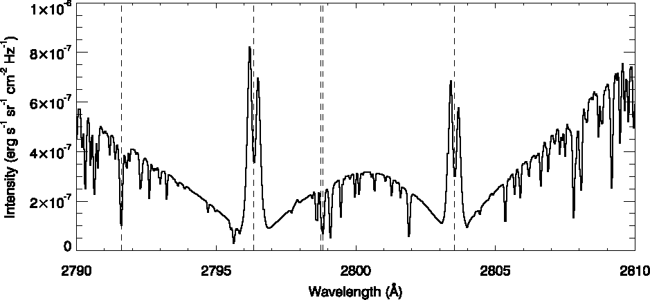
Figure 1: Averaged Sun-centre spectrum from 29 September 2013, used in the calculation of incident profiles in the Mg ii updates to the PROM code. Dashed lines indicate locations of the five Mg ii lines of interest. From left to right: 2791.60 Å, 2796.35 Å (k), 2798.75 Å, 2798.82 Å, and 2803.53 Å (h).

An observation from 29 September 2013 is used here for the incident profiles, which consisted of one large raster centred on solar coordinate ($-1$″,$5$″). This raster is a coarse raster with a total of $64$ $2$″ steps, creating a full field of view of $127$″ $\times$ $120$″. The raster includes a full CCD readout, meaning that the entire spectral range of IRIS is available. Data is calibrated using standard SSW routines.

After calibration, the Mg ii spectra are averaged spatially over the entire extent of the raster. The spatially averaged NUV spectrum around the Mg ii lines is shown in Figure 1, with positions of the five Mg ii lines marked with dashed lines. From left to right, the lines are 2791.60 Å (subordinate), 2796.35 Å (k), 2798.75 Å (subordinate), 2798.82 Å (subordinate), and 2803.53 Å (h).

Our code requires half profile inputs for each line, which are assumed to be symmetrical about the line core. For the h and k lines the profiles are taken from line centre out to $3$ Å in both directions, limited by the shape of the continuum between h and k. As can be seen in Figure 1 the red and blue peaks of the h and k lines are not symmetrical; the blue peak is larger in both cases. To deal with this asymmetry the half profiles are formed by averaging the blue and red sides of the line together. In the wings of these lines, there are a number of absorption lines which are not needed in the calculation of the emergent Mg ii h and k profiles. To help deal with these, smoothing is applied to the wings after averaging the profiles beyond the k₁ and h₁ positions, and a linear interpolation is performed in the far wings of the profiles in order to remove the remaining absorption features. The final incident half profiles for the h and k lines are shown in Figure 2.

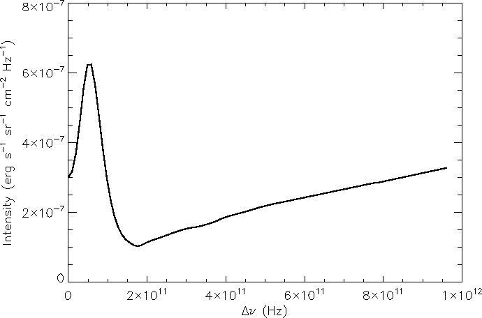
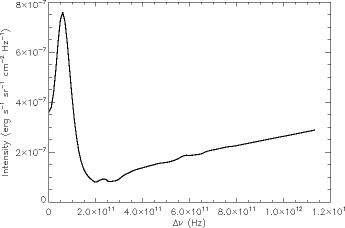
Figure 2: Incident half line profiles for Mg ii h (top) and k (bottom) lines. Line cores ($\Delta\nu\sim 0-2\times 10^{11}$ Hz) are the average of the blue and red sides of the profile only. Above $\Delta\nu\sim 2\times 10^{11}$ Hz profiles are averaged and smoothed. Absorption lines in the far wings are removed by interpolating between points in the continuum.

A detailed line profile for the subordinate lines is not required because the incident radiation does not play a large role in the emergent profile. An approximation is made such that they can be described by a single representative intensity value at the centroid position of each line. This intensity value is taken as the value of the continuum at the line centroid positions – $4.35\times 10^{-7}$ erg s^-1 cm^-2 sr^-1 Hz^-1 for 2791.60 Å, $2.49\times 10^{-7}$ erg s^-1 cm^-2 sr^-1 Hz^-1 for 2798.75 Å, and $2.54\times 10^{-7}$ erg s^-1 cm^-2 sr^-1 Hz^-1 for 2798.82 Å.

The photoionisation rates in the Mg ii continua are calculated using the internal radiation field resulting from the hydrogen calculations.

2.4 Grids of prominence model atmospheres

A basic non-LTE 1D model can act as an easy reference for the interpretation of observations. This allows a comparison to be made between observables, such as the line profile characteristics, and the prominence physical parameters, such as temperature, gas pressure, or optical thickness. We use two types of prominence model atmospheres, which are described below.

2.4.1 Isothermal isobaric models

To explore the influence of the relevant physical parameters for the formation of the Mg ii h and k lines in solar prominences, a total of $252$ isothermal isobaric models are considered; the model parameters are shown in Table 1.

Table 1: Model parameters for the grid of 1D isothermal isobaric models. $T$ denotes temperature, $P$ is gas pressure, and $D$ is slab thickness. $v_{T}$ and $H$ are microturbulent velocity and prominence height above the solar surface, respectively.

Parameter	Unit	Value
$T$	K	$6000$, $8000$, $10000$,
		$15000$, $20000$, $25000$,
		$30000$, $35000$, $40000$
$P$	dyne cm-2	$0.01$, $0.02$, $0.05$, $0.1$,
		$0.2$, $0.5$, $1$
$D$	km	$200$, $500$, $1000$, $2000$
$v_{T}$	km s-1	$5$
$H$	km	$10000$

Nine temperatures between $6000$ K and $40000$ K are considered here, as the Mg ii lines are formed at chromospheric temperatures of $\sim 30000$ K according to CHIANTI v8.0 (Dere et al., 1997; Del Zanna et al., 2015). The figure of $30000$ K for the formation of Mg ii lines comes from calculations considering purely collisional excitation and does not take into account radiative excitation, which is important in prominences. Radiative effects can have a large effect on the population of the h and k levels, and the formation of the corresponding resonance lines. In other words, the h and k lines can form at lower plasma temperatures of around $10000$ K (Leenaarts et al., 2013a, b). We use seven gas pressures between $0.01$ and $1$ dyne cm^-2. Slab thicknesses of $200$, $500$, $1000$, and $2000$ km are considered. For these isothermal isobaric models the turbulent velocity and prominence height are again kept constant at $v_{T}=5$ km s^-1 and $H=10000$ km, respectively.

2.4.2 PCTR models

The Mg ii lines are formed at plasma temperatures around $10000-15000$ K, but an isothermal model with that temperature does not best describe the prominence, as we know that there is lower temperature plasma in the prominence too. Therefore, it is more sensible to consider models that have a prominence-to-corona transition region (PCTR) between the cool, dense core and the hot, tenuous corona. The PCTR models here follow the temperature and pressure gradients described by Anzer & Heinzel (1999). Equations (3) and (4) show the expressions for the pressure, $P(m)$, and temperature, $T(m)$, as a function of column mass $m$ across the PCTR:

$$P(m)=4P_{c}\frac{m}{M}\left(1-\frac{m}{M}\right)+P_{0}\ ,$$ (3)

$$T(m)=T_{\mathrm{cen}}+(T_{\mathrm{tr}}-T_{\mathrm{cen}})\left(1-4\frac{m}{M}\left(1-\frac{m}{M}\right)\right)^{\gamma}\ .$$ (4)

The pressure at the outer edge of the PCTR is $P_{0}$, while at the centre of the slab it is $P_{\mathrm{cen}}=P_{c}+P_{0}$. The central temperature is $T_{\mathrm{cen}}$, and the temperature at the outer edge of the PCTR is $T_{\mathrm{tr}}$. In Eq. (4), $\gamma$ is a free parameter, with $\gamma\geq 2$. When $\gamma$ is small, the PCTR is extended (low temperature gradient), and when $\gamma$ is large, the PCTR is narrow (large temperature gradient).

For the PCTR models considered here, the $T$ and $P$ values listed in Table 1 are taken to be the range of central pressure and temperatures, $P_{\mathrm{cen}}$ and $T_{\mathrm{cen}}$, respectively. Column mass values range from around $1\times 10^{-7}$ g cm^-2 to around $1\times 10^{-3}$ g cm^-2. The temperature $T_{\mathrm{tr}}$ is set with a value of $1\times 10^{5}$ K, with $P_{0}$ taking a value of $0.01$ dyne cm^-2. The parameter $\gamma$ is varied and has three values: $2$, $5$, and $10$. The microturbulent velocity is again kept at a constant $5$ km s^-1, and the prominence height at $10000$ km. A summary of the parameters used in the PCTR models is presented in Table 2.

Table 2: Parameters used in the grid of models with a PCTR: $T_{\mathrm{cen}}$ is central temperature, $T_{\mathrm{tr}}$ is temperature at the edge of the slab, $P_{\mathrm{cen}}$ is the pressure at the centre of the slab, $P_{0}$ is pressure at the edge of the slab, $M$ is column mass, $\gamma$ controls PCTR size, $v_{T}$ is microturbulent velocity, and $H$ is height above the solar surface.

Parameter	Unit	Value
$T_{\mathrm{cen}}$	K	$6000$, $8000$, $10000$,
		$15000$, $20000$, $25000$,
		$30000$, $35000$, $40000$
$T_{\mathrm{tr}}$	K	$100000$
$P_{\mathrm{cen}}$	dyne cm-2	$0.01$, $0.02$, $0.05$, $0.1$,
		$0.2$, $0.5$, $1$
$P_{0}$	dyne cm-2	$0.01$
$M$	g cm-2	$1\times 10^{-7}-1\times 10^{-3}$
$\gamma$		$2$, $5$, $10$
$v_{T}$	km s-1	$5$
$H$	km	$10000$

In total there are $252\times 3=756$ possible unique PCTR models. This extended grid covers values that are not necessarily all relevant to typical solar prominence conditions, but will allow us to have a good understanding of the formation mechanisms of Mg ii lines in these structures.

3 Results

With spectrometers such as IRIS, detailed line profiles of the Mg ii lines are obtainable, meaning that line features (central reversals, line intensities, etc.) can be measured in prominences with a high spectral resolution. This section aims to explore whether any of these observables are related to the prominence parameters (temperature, gas pressure, slab thickness, optical thickness). Observable characteristics include the k-to-h line ratio (defined as the ratio of frequency-integrated intensities of the two lines), or the k (or h) line reversal level, also referred to generally as $I_{\mathrm{p}}/I_{0}$ (i.e. the ratio of specific intensities at the peak, $I_{\mathrm{p}}$, to those at the line centre, $I_{0}$) and specifically for h and k as $I(\text{h}_{2})/I({h}_{3})$ and $I(\text{k}_{2})/I({k}_{3})$, respectively. In the following, we present results concerning correlations between observables and model parameters, and correlations between Mg ii and H i intensities. We start by exploring how observable properties of the Mg ii h and k lines are related to each other. We focus on the following observables:

• frequency-integrated intensities of the Mg ii h and k lines, and of the H i Ly$\alpha$ and H$\alpha$ lines;

• Mg ii h and k reversal levels;

• emergent Mg ii h and k line profiles;

• Mg ii k/h line ratio.

Figure 3 shows relationships between observable parameters for h versus k for all isothermal, isobaric (top row) and PCTR (three bottom rows for each of the three $\gamma$ values) models.

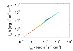
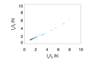
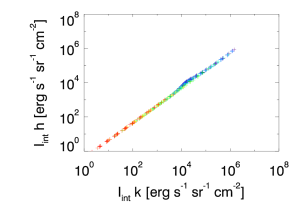
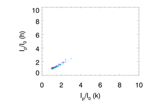
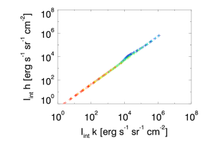
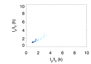
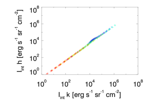
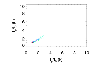
Figure 3: Correlations between observable properties of the Mg ii h and k lines. Left: Correlation between frequency-integrated intensities of the Mg ii h and k lines. Right: Correlation between Mg ii h and k reversal levels. Top row: Points are for all isothermal isobaric models. Three bottom rows: Points are for all PCTR models. Second row: $\gamma=2$. Third row: $\gamma=5$. Bottom: $\gamma=10$. Colour indicates temperature, increasing from purple to red.

The plots of the frequency-integrated intensity of Mg ii h against the frequency-integrated intensity of Mg ii k show an almost perfect power-law relationship, with a power-law index of $1.01$ in the $\gamma=10$ case, and $1.02$ in all the other cases, as expected from the ratio of oscillator strengths of the h and k lines. However there is a small ‘bump’ at around $I_{\mathrm{int}}$ (k) = $10^{4}$ erg s^-1 sr^-1 cm^-2 corresponding to central temperatures lower than 10000 K. This departure from linearity can be explained by considering the optical thickness of the lines (see below). The optical thickness is defined as usual, and measures the absorption of radiation across the slab width

$$\tau=\int_{0}^{D}\alpha\mathrm{d}s\ ,$$

with $D$ the slab width, $\alpha$ the absorption coefficient in a given line, and $\mathrm{d}s$ a small path element.

The right-hand panels of Fig. 3 show the correlation between reversal levels of the h and k lines. There is a roughly linear relationship between h line reversal level and k line reversal level. Most points are clustered at lower reversal levels ($\sim 1-2$), with relatively few models showing a high reversal level in either line. We see a slightly different spread of values between the PCTR and the isothermal isobaric models. In the PCTR case, there are no models with higher ($>4$) reversal levels in either line for any $\gamma$ value. This indicates that the inclusion of a PCTR inhibits the creation of extremely deep central reversals in the line profiles; the presence of a PCTR near the surface of the slab changes the source function in the slab, due to the larger effect of collisional excitation.

Figure 4 presents the h and k frequency-integrated intensities versus the optical thickness of the line for all isothermal isobaric and PCTR models.

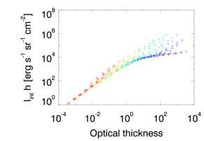
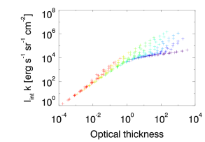
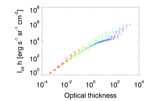
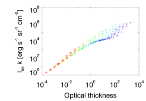
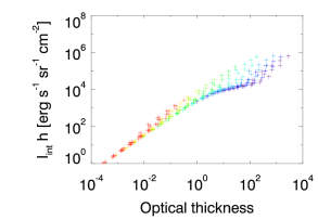
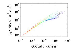
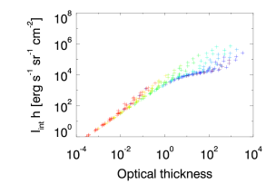
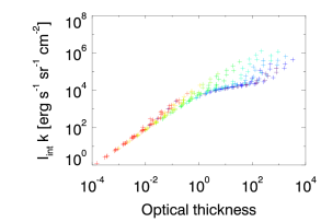
Figure 4: Plots of frequency-integrated intensity against optical thickness for the Mg ii resonance lines. Left: Mg ii h. Right: Mg ii k. Top row: Points are for all isothermal isobaric models. Three bottom rows: Points are for all PCTR models. Second row: $\gamma=2$. Third row: $\gamma=5$. Bottom: $\gamma=10$. Colour indicates temperature, increasing from purple to red.

The ‘bump’ in Figure 3 corresponds to the intensity where the h and k lines become optically thick, and the models with the highest optical thickness can be found to have a frequency-integrated intensity around $10^{4}$ erg s^-1 sr^-1 cm^-2 in both lines. A small number of models deviate from this value, having higher intensities for optically thick models, creating a scatter of points in Figure 4. These mostly continue the approximate power law seen at lower optical thicknesses and frequency-integrated intensities. The optical thickness for the PCTR models is similar to that of the isothermal isobaric values, but at high optical thicknesses there is some variation. In the PCTR models, the higher optical thickness values are only found at higher frequency-integrated intensities: the relation is more linear and there is less ‘flattening’ of the scatter plots at $\sim 10^{4}$ erg s^-1 sr^-1 cm^-2. This has an effect on the resulting line profiles (Fig. 6).

Importantly, as shown in Figure 5, optical thicknesses higher than around $10$ are where the h and k lines begin to become reversed. For PCTR models, this occurs for models with $T_{\mathrm{cen}}<25000$ K. Only the PCTR models where $\gamma=2$ are presented here, as they represent the most extended PCTR case.

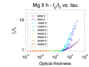
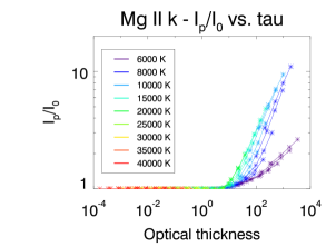
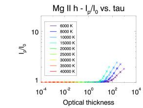
Figure 5: Reversal level against line optical thickness of Mg ii h (left), and Mg ii k (right). Top row: Isothermal isobaric models. Bottom row: Models with a PCTR and $\gamma=2$. Colour indicates temperature, increasing from purple to red.

A reversal at line centre results in a reduction of the frequency-integrated intensity compared to an equivalent non-reversed profile, which accounts for the flattening of the plots in Figure 4. Differences in the optical thickness for the h and k lines means there will be different possible relative h and k intensity values depending on the model. This then causes the small departure from power-law linearity seen in Figure 3. Figure 5 illustrates again that the inclusion of a PCTR inhibits the creation of deep central reversals.

3.1 Correlations between observables and model parameters

Figure 6 shows the emergent Mg ii k profiles for the isothermal isobaric and PCTR models, with each panel showing all pressure $P$ and slab thickness $D$ combinations for a single temperature. Line profiles for PCTR models are only shown for $\gamma=2$.

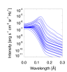
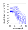
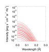
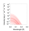
Figure 6: Emergent half-line Mg ii k profiles. The first three columns show isothermal isobaric models; the last three columns show PCTR models with $\gamma=2$. Each panel is colour-coded to show a different temperature: $6000$ K (purple), $8000$ K (dark blue), $10000$ K (light blue), $15000$ K (teal), $20000$ K (green), $25000$ K (lime green), $30000$ K (yellow), $35000$ K (orange), and $40000$ K (red). Intensities generally increase for higher pressure and slab thickness.

Notably, in the isothermal isobaric case, lower temperature models ($\leq 20000$ K) show a mix of reversed and non-reversed profiles, whereas higher temperature models ($>20000$ K) do not show any line reversals. It will therefore be worth exploring these high-temperature models in more detail to gauge their relevance to observations. Line centre intensities for models with low central temperature ($T_{\mathrm{cen}}=6000,8000,10000$ K) have a much larger spread of values for the PCTR models than the isothermal models. This occurs because there is plasma with much higher temperatures than the stated core temperature in the slab, which is due to the presence of the PCTR. A value of $\gamma=2$ means that there will be more high-temperature plasma nearer the slab centre. As $\gamma$ becomes larger the PCTR becomes narrower, and the solutions for high $\gamma$ should converge to the isothermal case (Labrosse & Gouttebroze, 2004). As a consequence, the central reversals seen in the h and k profiles should become deeper as $\gamma$ increases. The effects of this are not seen, however, for the three values of $\gamma$ considered here, as seen in the right panels of Figure 3. Values of $\gamma$ much higher than 10 (maximum value adopted here) are required to see this effect (Labrosse & Gouttebroze, 2004; Heinzel et al., 2014).

To explore the relevance of high-temperature models to observations in more detail, we present in Figure 7 the emergent half h and k profiles for isothermal isobaric models with $T\geq 15000$ K at one slab thickness, $D=1000$ km, and two gas pressures, $P=0.1$ dyne cm^-2 (solid lines), and $P=0.5$ dyne cm^-2 (dashed lines).

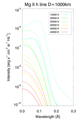
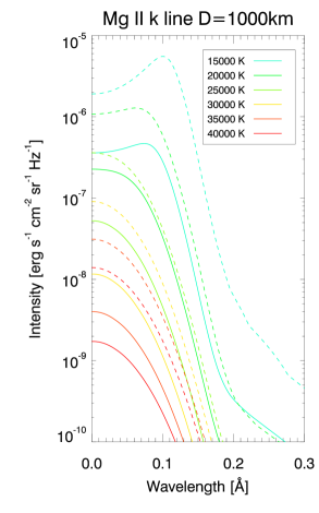
Figure 7: Half-line emergent profiles for the Mg ii h (left) and k (right) lines from isothermal isobaric models with $T\geq 15000$ K. All profiles are from models with $D=1000$ km. Profiles for two pressures are shown, with $P=0.1$ dyne cm^-2 (solid lines) and $P=0.5$ dyne cm^-2 (dashed lines). Temperatures are colour-coded: $15000$ K (black), $20000$ K (maroon), $25000$ K (red), $30000$ K (pink), $35000$ K (orange), and $40000$ K (yellow).

Each temperature is given a different colour to distinguish them. The profiles are reversed for the $15000$ K models, becoming flat-topped at $20000$ K, and are not reversed above $25000$ K; this can already be seen in Figure 5 where all high-temperature models do not show central reversals. Also, as the temperature increases the line intensity decreases. This can be seen for line centre intensity in Figure 7, and also for the frequency-integrated line intensity which is plotted as a function of temperature in Figure 8.

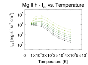
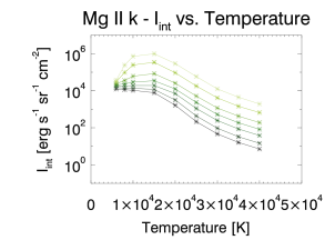
Figure 8: Plots of frequency-integrated intensity against temperature for isothermal isobaric models with $D=1000$ km. Colour indicates pressures of (from dark to light) $0.01$, $0.02$, $0.05$, $0.1$, $0.2$, $0.5$, and $1$ dyne cm^-2. Left: Mg ii h. Right: Mg ii k.

Figure 8 shows plots for only isothermal isobaric models with $D=1000$ km, but includes all the pressures indicated by the colour gradient. These plots mostly have peaks at a temperature of around $10000-15000$ K for higher pressure models, around the formation temperature of Mg ii (Leenaarts et al., 2013a, b). In these cases, the peak occurs where collisional processes would be expected to begin to dominate over radiative ones. At low pressures the emission seen will mostly be the result of resonant scattering of photons from the solar disc, causing radiative excitation of the lower levels of the h and k lines. As the pressure increases, the collisional processes become more important so the line intensity generally increases with respect to lower pressure models. Above $15000$ K a larger proportion of Mg ii is ionised to Mg iii so there is less Mg ii in the relevant energy levels for the h and k transitions, and the intensity drops off as temperature increases.

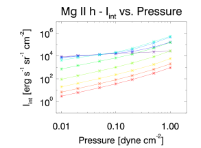
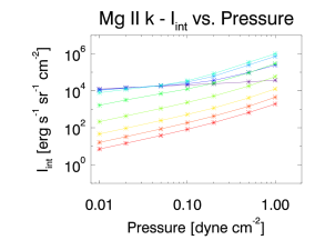
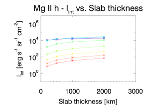
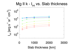
Figure 9: Plots of frequency-integrated intensity for Mg ii h (left) and Mg ii k (right) against gas pressure (top) and slab thickness (bottom) for isothermal isobaric models. Pressure plots are for models with $D=1000$ km, slab thickness plots are for models with $P=0.1$ dyne cm^-2. Colour indicates temperature, increasing from purple to red.

Figure 9 shows plots of frequency-integrated intensity against gas pressure and slab thickness for the Mg ii h and k lines in the case of isothermal isobaric models. The top panels are shown for one slab thickness ($D=1000$ km) and the bottom panels are shown for one gas pressure ($P=0.1$ dyne cm^-2). Temperatures are colour-coded, with low temperatures having darker colours and high temperatures having lighter colours. The frequency-integrated intensities of the h and k lines increase with gas pressure and with slab thickness. These plots clearly show, at the temperatures most representative of prominence conditions, that these dependencies are weak, which is due to the relatively high optical thickness of the plasma. The temperature structure seen in Figure 8 (peaked around $10000-15000$ K) can also be identified in these plots.

The results shown here indicate that the formation temperature of the Mg ii lines estimated from purely collisional excitation, $30000$ K (Sigut & Pradhan, 1995; Dere et al., 1997; Del Zanna et al., 2015), is an overestimation for the case of solar prominences. This was also found for the chromosphere (Leenaarts et al., 2013a, b), where the importance of radiative excitation means that photons of Mg ii h and k are created much more frequently at lower temperatures, around $10000$ K. The effects of ionisation from Mg ii to Mg iii at $30000$ K are also considerable, with the population of the Mg ii ground level being reduced to the stage that the plasma becomes optically thin at h and k wavelengths, and no central reversals are seen.

Our two grids of models provide a large extension to the $27$ isothermal isobaric models presented by Heinzel et al. (2014). However, models with higher central temperatures ($>20000$ K) present non-reversed profiles with extremely low peak intensity values, below $10^{-7}$ erg s^-1 cm^-2 sr^-1 Hz^-1 and as low as $5\times 10^{-11}$ erg s^-1 cm^-2 sr^-1 Hz^-1 for some of the highest temperature slabs. They also show no central reversal above $20000$ K. This does not seem to match observations, where central reversals are observed, and for non-reversed profiles line-centre intensities of more than $10^{-7}$ erg s^-1 cm^-2 sr^-1 Hz^-1 are recovered (e.g. Levens et al., 2017). It is therefore not necessary to consider models with extremely high temperatures in comparison to observations, but it appears to be reasonable to consider models with temperatures up to $\sim 20000$ K.

The k/h line ratio is one of the simplest parameters to calculate from observations, so understanding how it is related to the physical parameters of the plasma could potentially be very powerful for analysis. Figure 10 shows the k/h line ratio against temperature, pressure, slab thickness, and optical thickness for isothermal isobaric models and for PCTR models with $\gamma=2$.

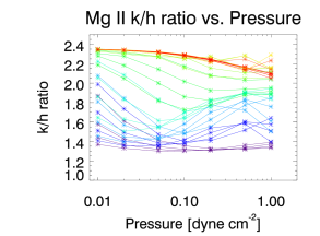
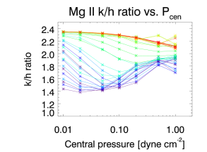
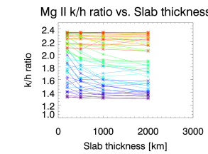
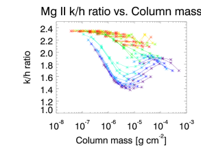
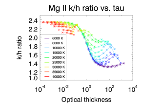
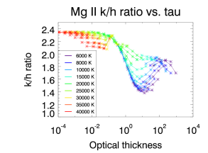
Figure 10: Plots of the Mg ii k/h line ratio against physical parameters for the isothermal isobaric (left column) and PCTR (with $\gamma=2$, right column) models. First row: k/h line ratio vs. $T$ (left) or $T_{\mathrm{cen}}$ (right), colour scale indicates pressure. Second row: k/h line ratio vs. $P$ (left) or $P_{\mathrm{cen}}$ (right), colour scale indicates temperature. Third row: k/h line ratio vs. $D$ (left) or $M$ (right), colour scale indicates temperature. Bottom row: k/h line ratio vs. $\tau_{\mathrm{h}}$, colour scale indicates temperature.

Plotting the k/h line ratio against temperature (Fig. 10, first row) reveals that, for all pressures, the k/h line ratio increases approximately linearly with temperature up to around $25000$ K, where the k/h line ratio saturates between $2$ and $2.4$. This suggests that for lower (more realistic) temperatures the k/h line ratio is a close analogy to temperature, regardless of slab thickness or pressure. The plots of k/h line ratio against pressure (second row) do not show any significant correlations in the isothermal isobaric case. The central pressure has a larger effect on the k/h line ratio for PCTR models than in the isothermal isobaric case. At low temperatures, the k/h line ratio may increase with central pressure, whereas for high-temperature models the opposite is true. It is also interesting to note that observed values of k/h line ratios around $1.4$ are only seen for the lowest pressure PCTR models, where $P_{\mathrm{cen}}=0.01,0.02$ dyne cm^-2. The plots of k/h line ratio against slab thickness (third row, left) do not show any significant correlations in the isothermal isobaric case. The relationship between k/h line ratio and column mass for PCTR models gives a totally different picture and is similar to that of the k/h line ratio and optical thickness. The bottom row of Figure 10 shows the k/h line ratio against optical thickness of the h line; the k/h line ratio against k line optical thickness is not shown as it is almost identical. There is a general trend that shows lower optical thickness has a larger k/h line ratio, with higher optical thicknesses corresponding to lower k/h line ratios. The transition between the two cases is at $\tau$ values around the transition between optically thin and optically thick. There are some diversions from this trend (so there is some model dependence), but generally the k/h line ratio does appear to depend on the optical thickness, and when the lines are optically thin ($\tau<1$) the k/h line ratio is higher than $2$. In the PCTR case, there are fewer models at k/h line ratios of $1.4$ than in the isothermal isobaric case ; that ratio appears to correlate only to a few models where the optical thickness is around $10$, corresponding to those models with low $P_{\mathrm{cen}}$, mentioned previously.

As mentioned earlier, the reversal level of the h and k lines is heavily dependent on the optical thickness of the lines, as seen in Figure 5. Exploring how the reversal level is related to other parameters is useful for narrowing down the physical prominence conditions that give rise to the observed profiles. Figure 11 shows plots of h and k line reversal levels against central temperature, central gas pressure, and slab thickness or column width for isothermal isobaric models (first two columns) and PCTR models with $\gamma=2$ (last two columns).

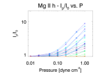
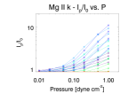
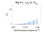
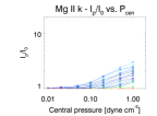
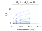
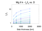
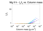
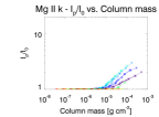
Figure 11: Plots of reversal level of the Mg ii h line (first and third columns) and k line (second and fourth columns) against physical parameters for the isothermal isobaric models (first two columns) and the PCTR models with $\gamma=2$ (last two columns). Top: Reversal level vs. central temperature, colour scale indicates pressure. Middle: Reversal level vs. central pressure, colour scale indicates temperature. Bottom: Reversal level vs. slab thickness (for isothermal isobaric models) or column mass (for PCTR models), colour scale indicates temperature.

The lower maximum reversal level for PCTR models as compared to isothermal isobaric models is clearly seen in all plots. The reversal level vs. temperature plots (top panels) show that the reversal level of both h and k lines is heavily dependent on temperature, but also on gas pressure (shown by the green colour gradient). In terms of temperature, the reversal level is greatest at around $8000-10000$ K, dependent on the model. These plots also generally show that the level of reversal increases with pressure (see middle row). The bottom panels of Figure 11 show that for reversed profiles the slab thickness does have an effect on the level of reversal seen in the emergent profile from isothermal isobaric models, with the largest line reversal levels only being found for the thickest prominence slabs. Reversal level as a function of optical thickness was already discussed in Fig. 5, where only models with optical thickness higher than $\sim 10$ show a central reversal. Column mass (used in PCTR models) is related to reversal level in a similar way to optical thickness. Only column masses above $5\times 10^{-6}$ g cm^-2 have a central reversal, and again it is only lower temperature models that show any reversal.

3.2 Correlations between Mg ii and H i intensities

It is also interesting to note how the Mg ii lines correlate with intensities emitted in hydrogen lines. Figure 12 shows how the intensity in the k lines depends on the Ly$\alpha$ and H$\alpha$ intensities. The corresponding diagram for the Ly$\beta$ line is very similar to that of Ly$\alpha$ and is therefore not shown here. In Fig. 12, each colour represents a different range of mean temperatures, where the mean temperature is the weighted-mean of the temperature along the line of sight as in Labrosse & Gouttebroze (2004). Of course, the mean temperature has the same value as the central temperature for isothermal models. In the case of PCTR models, however, the mean temperature can be significantly higher than the temperature at the slab centre. In the PCTR models used here (Table 2), the lowest mean temperature is nearly 10500 K.

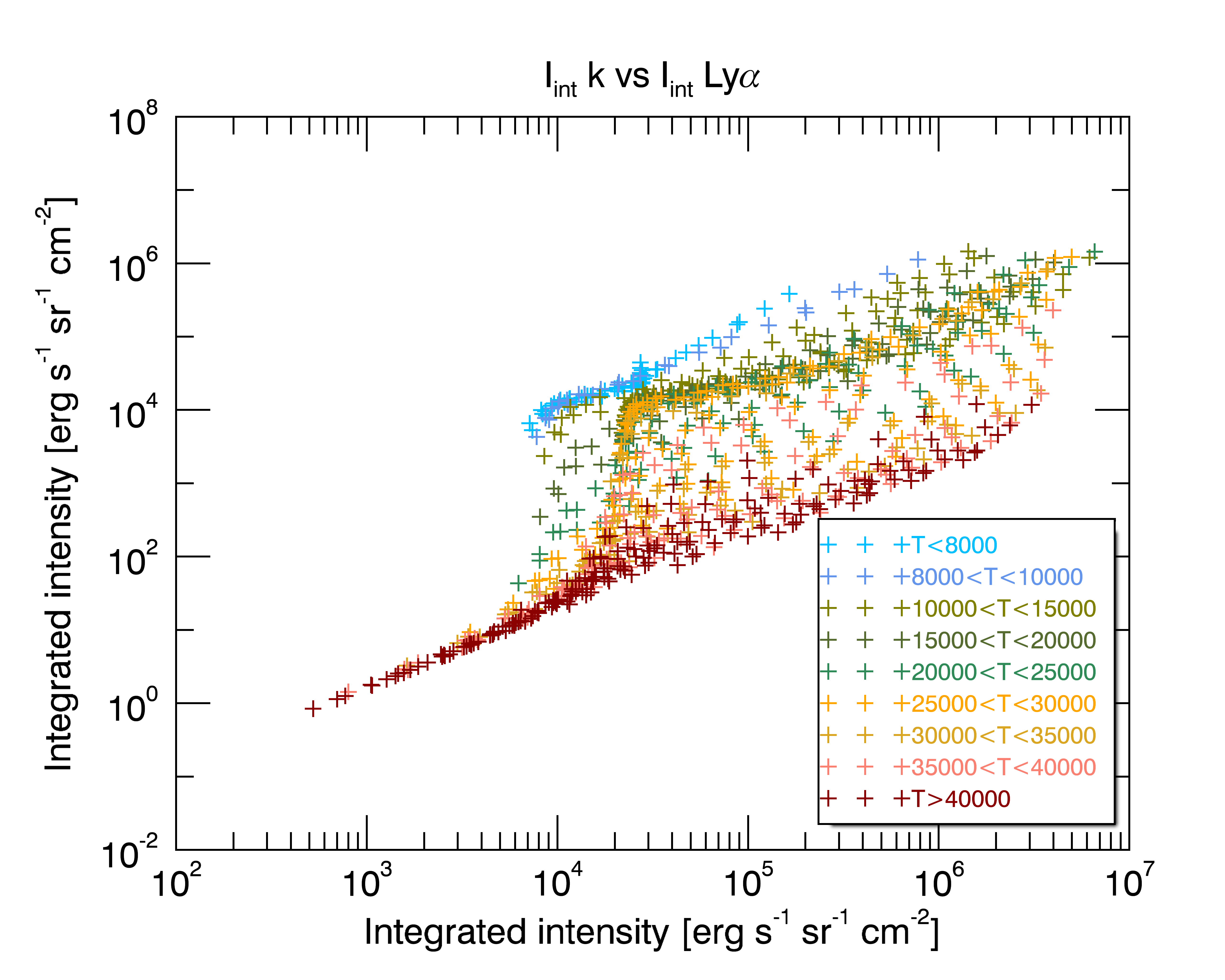
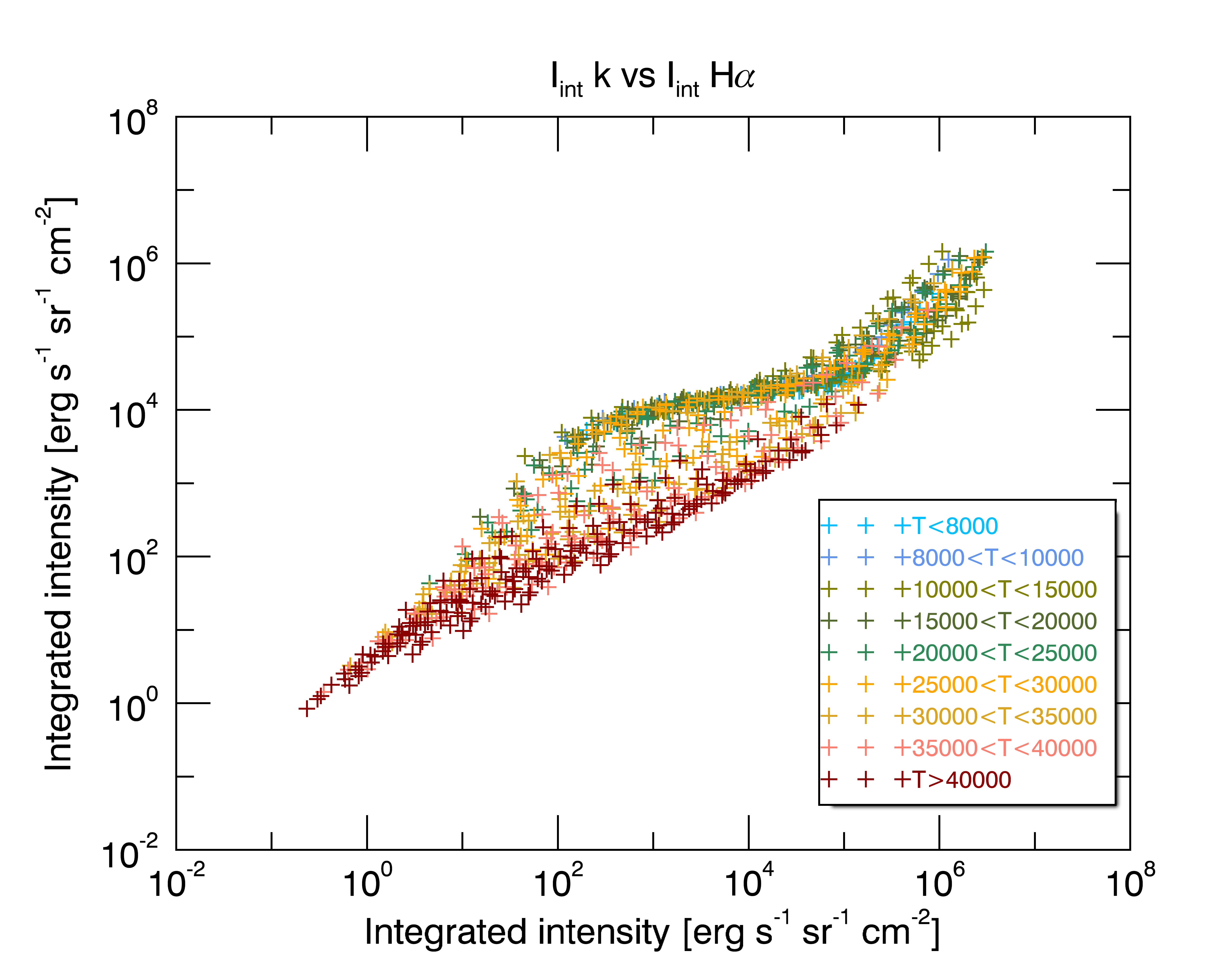
Figure 12: Frequency-integrated intensity in the k line as a function of the Ly$\alpha$ (top) and H$\alpha$ (bottom) frequency-integrated intensities. The results are plotted for isothermal and for isobaric models, and for models with a PCTR. Each colour corresponds to a given range of mean temperatures.

In the top panel of Fig. 13, we show the relation between the k line frequency-integrated intensity and the emission measure, defined here as $\mathrm{EM}=n_{e}^{2}D$. If the thickness of the prominence slab (in other words the extent of the observed prominence along the line of sight) can be estimated, a good correlation between the two quantities means that the k line intensity provides a way to measure the electron density in the prominence.

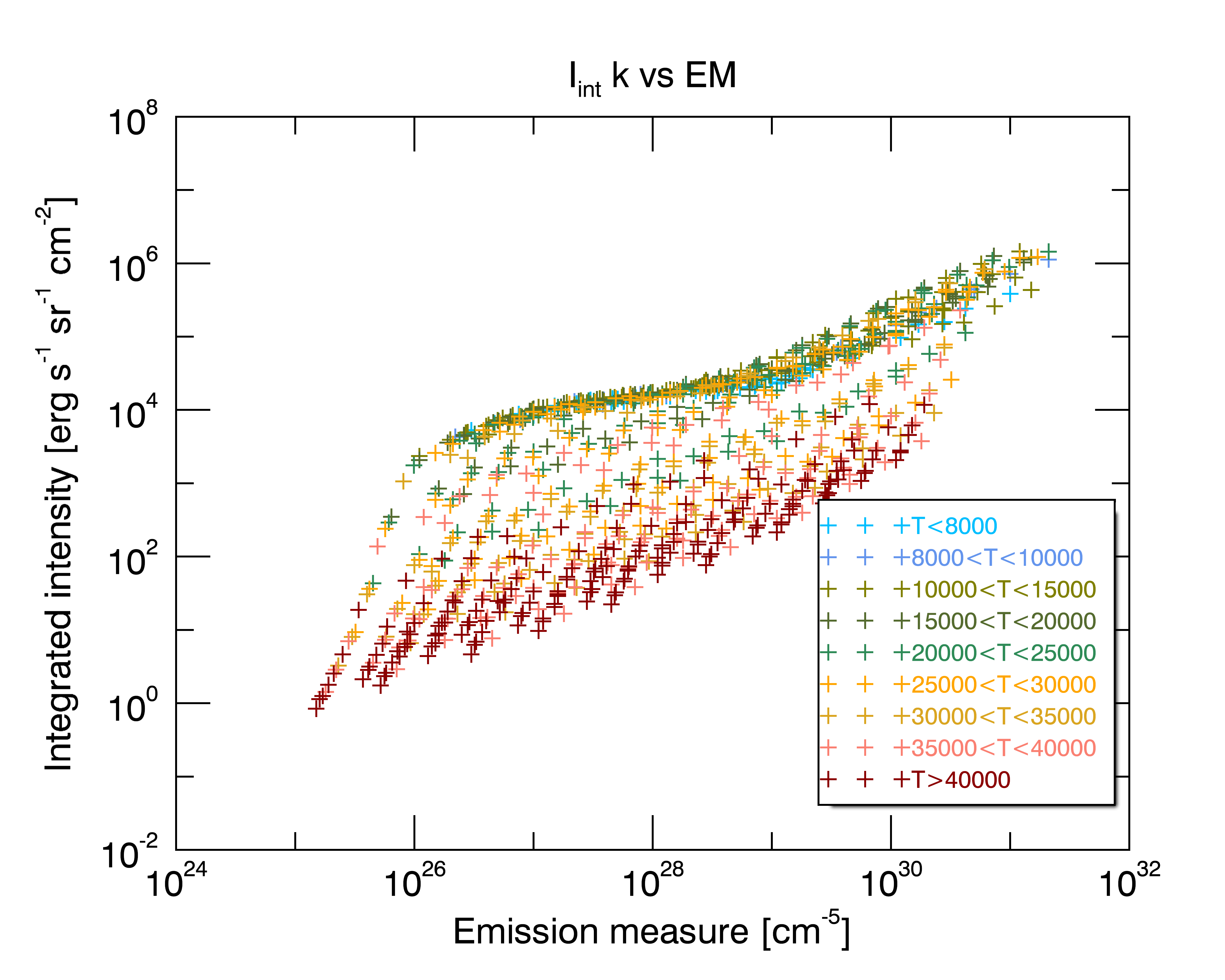
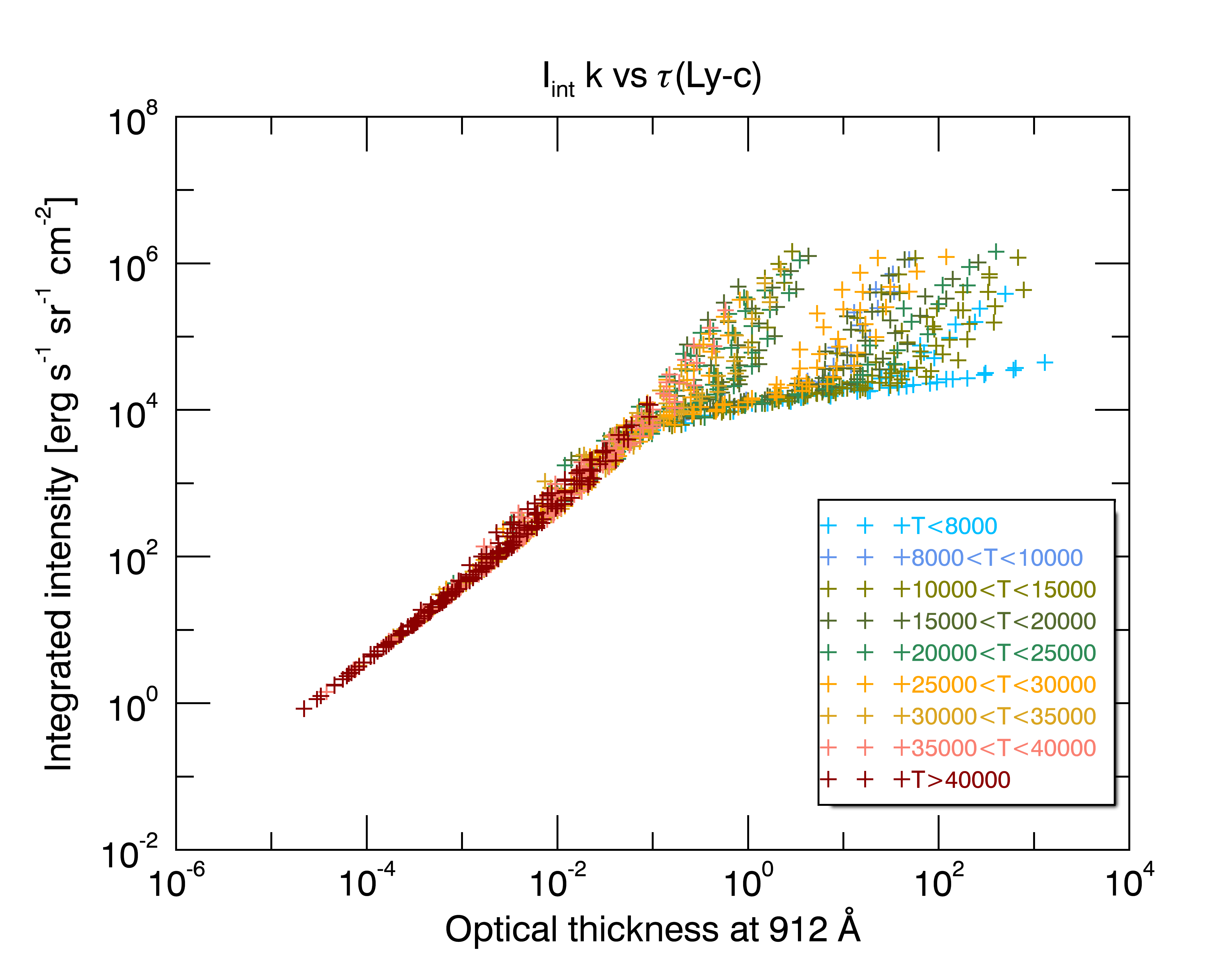
Figure 13: Frequency-integrated intensity in the k line as a function of emission measure (top) and the optical thickness at the head of the Lyman continuum (912 Å). The results are plotted for both isothermal and isobaric models, and models with a PCTR. Each colour corresponds to a given range of mean temperatures.

We immediately note that the trend shown in the top panel of Fig. 13 is similar to that seen in the bottom panel of Fig. 12, namely the correlation between the k and H$\alpha$ line intensities. This is not surprising as we know that a strong relation between H$\alpha$ intensities and emission measure was found in 1D isothermal isobaric models (Gouttebroze et al., 1993). This correlation still exists for PCTR models. Here we consider a broader grid of models than in GHV, and H$\alpha$ intensities generally become lower as the mean temperature of the model increases. This is what produces the apparent spread in these plots.

We also show the relation between the k line intensity and the optical thickness at the head of the Lyman continuum (912 Å) in the bottom panel of Fig. 13. The latter gives us an idea of the penetration of the incident radiation in the slab, in particular with less ionising radiation penetrating deep in the slab for models where the plasma is optically thick at 912 Å. We see in this plot that the intensities in the Mg ii k line (and of the h line, too) will be first determined by the amount of external radiation received by the ions in the prominence for the coolest models. As the mean temperature increases, the collisions become more important in the formation of the lines, while at the same time letting more radiation penetrate (as the temperature increase results in a lower optical thickness at 912 Å). For very high temperatures, higher than 30000 K, all our models are optically thin in the Lyman continuum, while Mg ii is depleted and populates Mg iii.

As noted earlier, we expect the most representative prominence models to have temperatures lower than 25000 K, and these results indicate that we can expect good correlations between the Mg ii k line intensities and the intensities of hydrogen lines, as well as the emission measure.

4 Summary and conclusion

This study is dedicated to developing prominence models of the Mg ii h and k resonance lines, and using them to investigate how these lines behave under a wide range of physical conditions. Since the launch of IRIS, the Mg ii h and k lines have been well studied and modelled in the chromosphere (Leenaarts et al., 2013a, b), in flares (e.g. Kerr et al., 2016), and in prominences (Heinzel et al., 2014, 2015). The Heinzel et al. (2014, HVA) grid of prominence Mg ii models explored $27$ isothermal isobaric models and investigated the inclusion of a PCTR to some of their models as well. The goal of the present work is to extend that grid of models in order to more fully understand the behaviour of the Mg ii h and k lines.

The atomic model of magnesium used here was constructed using standard atomic data for a five-level plus continuum Mg ii atom. Incident radiation was determined using IRIS quiet-sun profiles for the Mg ii h and k lines, as well as continuum-level intensities for the three Mg ii subordinate lines. Our results are qualitatively similar to those from HVA.

An extended grid of 1D models was designed in order to investigate the effects of higher temperatures and pressures on the emergent h and k line profiles. We then looked for correlations between observable line parameters (line frequency-integrated intensity, k/h line ratio, reversal level) and model parameters (temperature, pressure, and slab thickness or total column mass), as well as optical thickness. The frequency-integrated intensity of the h and k lines is closely related for all models, displaying a power-law relationship with a small ‘bump’ which is caused by the differences in the optical thickness of the h and k lines. Line reversal levels of both h and k are found to be closely related to optical thickness; only models where $\tau>10$ show any central reversal of the lines. The frequency-integrated intensity is also related to the optical thickness of the lines for both h and k, with the relationship changing at the transition between optically thin and optically thick.

Investigating higher temperature models ($T\geq 15000$ K) reveals firstly that there are no central reversals found for models above $20000$ K. Secondly, the line centre intensity decreases with temperature, down to values that are not observed in real prominences (within the instrumental sensitivity of IRIS). The cause of this decreased intensity is the increased amount of ionisation to Mg iii at these temperatures. Therefore, there is less Mg ii in the relevant energy states to produce photons that contribute to the h and k lines, causing a lower intensity in those lines. This indicates that extending the grid of isothermal isobaric models much past $\sim 20000$ K is not necessary, as the computed emergent line profiles do not reflect those observed. However, it will be useful to have a finer grid of models between $\sim 6000-15000$ K to properly investigate the differences in low-temperature cases.

Models with a prominence-corona transition region (PCTR) represent a significant improvement on isothermal isobaric slab models due to their temperature and pressure gradients between the cool prominence core and the hot surrounding atmosphere. Temperature and pressure gradients from Anzer & Heinzel (1999) are used here to represent the PCTR. The Mg ii h and k lines from PCTR models show similar inter-line relationships, and also a similar correlation with the line optical thickness to the isothermal isobaric cases. Considering the emergent line profiles themselves there are some notable changes. Primarily at low central temperatures ($<10000$ K) there is a much broader range of line-centre intensities recovered than in the isothermal case with the same central temperature. This is caused by the presence of higher temperature plasma in the PCTR, which causes more collisional excitation within the slab.

Some correlations are found between observable parameters of the Mg ii h and k lines (namely the k/h line ratio and the reversal level) and the temperature of the plasma slab, for both isothermal isobaric and PCTR models. For all pressures and slab thicknesses, the k/h line ratio increases approximately linearly with temperature, up to a point where the k/h line ratio saturates somewhere between $2$ and $2.4$, depending on the model. There is also some correlation between the k/h line ratio and the line optical thickness. In the isothermal isobaric case, for optically thin slabs (at higher $T$) the k/h line ratio is high, around $2$ to $2.4$, switching around $\tau=1$ to lower values of around $1.4$, mostly for low $T$ models. There are models that deviate from this trend, but generally the correlation seen is good. This is interesting in comparison with the IRIS observations presented in Levens et al. (2017), where k/h line ratio values closely scattered around a value of $1.4$ were found. From the model results shown here this indicates that the observed profiles are all optically thick, and the prominence temperatures are low ($\sim 6000-8000$ K). A similar trend is seen for models with a PCTR, but there is some deviation for models with high optical thickness. The observed trend indicates that only a small number of PCTR models can explain the observed k/h line ratio of $1.4$ – those with low pressure ($0.01$ or $0.02$ dyne cm^-2) and an optical thickness of around $10$. It remains to be seen which of these scenarios is more likely. However, the PCTR models are generally better at explaining observed line profiles (Schmieder et al., 2014; Heinzel et al., 2015). The reversal level of the h and k lines can also be used as an indicator of both the plasma temperature and pressure, with the largest peak-to-core ratios coming from models (isothermal isobaric and PCTR) with temperatures of $8000-10000$ K. Higher pressure models generally show higher reversal levels too; however, there is some model dependence of this. We find good correlations between the Mg ii k line intensities and the intensities of hydrogen lines, as well as with the emission measure.

These models represent a simplification of the physical conditions of prominence plasma, but are nonetheless a useful tool for investigating the prominence conditions with respect to the observed Mg ii h and k profiles. Although there is some improvement in moving from isothermal isobaric models to those with a PCTR, it will be useful to move to more complex multi-thread models for detailed comparisons to observations. The 1D isothermal isobaric and PCTR models presented here can be used as a base for these more complex prominence models, including ones that include 1D/2D multi-thread structures to attempt to replicate the fine structure and small-scale prominence dynamics that are observed (Gunár et al., 2007, 2008; Labrosse & Rodger, 2016).