The smallest nontrivial snarks of oddness 4

Abstract

The oddness of a cubic graph is the smallest number of odd circuits in a 2-factor of the graph. This invariant is widely considered to be one of the most important measures of uncolourability of cubic graphs and as such has been repeatedly reoccurring in numerous investigations of problems and conjectures surrounding snarks (connected cubic graphs admitting no proper $3$-edge-colouring). In [Ars Math. Contemp. 16 (2019), 277–298] we have proved that the smallest number of vertices of a snark with cyclic connectivity 4 and oddness 4 is 44. We now show that there are exactly 31 such snarks, all of them having girth 5. These snarks are built up from subgraphs of the Petersen graph and a small number of additional vertices. Depending on their structure they fall into six classes, each class giving rise to an infinite family of snarks with oddness at least $4$ with increasing order. We explain the reasons why these snarks have oddness 4 and prove that the 31 snarks form the complete set of snarks with cyclic connectivity 4 and oddness 4 on 44 vertices. The proof is a combination of a purely theoretical approach with extensive computations performed by a computer.

1 Introduction

This paper is a sequel of [8] where we have proved that the smallest number of vertices of a snark – a connected cubic graph whose edges cannot be properly coloured with three colours – which has cyclic connectivity $4$ and oddness at least $4$ is $44$. The purpose of the present paper is to show that there are precisely 31 such snarks, all of them having oddness exactly $4$, resistance $3$, and girth $5$. Together with [8], this paper provides a partial answer to the following question posed in [4, Problem 2], leaving open the existence of cyclically $5$-edge-connected snarks of oddness at least $4$ on fewer than 44 vertices:

Problem [4]. Which is the smallest snark (with cyclic connectivity $\geqslant 4$ and girth $\geqslant 5$) of oddness strictly greater than 2?

The oddness of a bridgeless cubic graph $G$ is the smallest number of odd circuits in a $2$-factor of $G$, and the resistance of $G$ is the smallest number of vertices (or edges) of $G$ whose removal yields a $3$-edge-colourable graph. Both invariants are important measures of uncolourability of cubic graphs and have been investigated by numerous authors [1, 5, 11, 12, 13, 15, 25]. One of the reasons why these invariants have recently received so much attention resides in the fact that snarks with large resistance or oddness may provide potential counterexamples to several profound conjectures such as the cycle double cover conjecture, the 5-flow conjecture, and others [11, 13, 14].

The set $\mathcal{M}$ of all $31$ snarks of order 44, cyclic connectivity $4$, and oddness $4$ has been constructed with the help of a computer. A detailed description of its members appears in Section 3 where we also give a computer-free proof that each of them has oddness at least $4$. The equality can be established easily by specifying a $2$-factor containing four odd circuits, which can be checked directly.

The snarks constituting the set $\mathcal{M}$ fall into six classes depending on their structure. A remarkable feature of the set is that all of them are built up from subgraphs of the Petersen graph and a small number of additional vertices. The verification that $\mathcal{M}$ is a complete set of snarks of order 44, cyclic connectivity $4$, and oddness at least $4$ combines purely mathematical considerations with extensive computations; the proof can be found in Section 4. Its mathematical part is essentially a mixture of edge-colouring and cyclic connectivity arguments. In the computational part we perform an operation that takes two cyclically $4$-edge-connected snarks $G_{1}$ and $G_{2}$ of order at most 36 and creates from them – in all possible ways – a cubic graph by either removing two adjacent vertices or two nonadjacent edges, and connecting the resulting $2$-valent vertices in $G_{1}$ with those in $G_{2}$. In total, more than $2\times 10^{13}$ graphs have been constructed and checked for oddness 4. The entire computational effort for this project amounts to 25 CPU years.

In Section 5 we analyse a sample of 887 152 cyclically $4$-edge-connected snarks of oddness $4$ whose orders range from 46 to 52, as well as 872 snarks of oddness $4$ with lower connectivity constructed in [9]. We evaluate various invariants for them such as resistance, perfect matching index, circumference, and others. The purpose of this investigation is to provide grounds for possible prediction of certain properties that snarks with higher oddness might have in general.

We conclude this paper with several open problems. At the end we append the adjacency lists of all 31 snarks constituting the set $\mathcal{M}$.

2 Preliminaries

This section collects the most basic definitions and notation needed for understanding the present paper. For a more detailed introduction to the topic we refer the reader to our preceding paper [8].

2.1. Graphs and multipoles. All graphs in this paper are finite and for the most part simple. However, for the sake of completeness we have to permit graphs containing multiple edges or loops, although these features will be usually excluded by the imposed connectivity or colouring restrictions. For a graph $G$ and a subgraph $H\subseteq G$ we let $|G|$ denote the number of vertices of $G$, and $G[H]$ the subgraph of $G$ induced by the vertex set of $H$.

Throughout this paper we use multipoles as a convenient tool for constructing graphs. Every edge of a multipole has two ends and each end can, but need not, be incident with a vertex. An edge which has one end incident with a vertex and the other not is called a dangling edge, and if neither end of an edge is incident with a vertex, it is called an isolated edge. An end of an edge that is not incident with a vertex is called a semiedge. A multipole with $k$ semiedges is called a $k$-pole. Two semiedges $s$ and $t$ of a multipole can be joined to produce an edge $s*t$ connecting the end-vertices of the corresponding dangling edges. Given two $k$-poles $M$ and $N$ with semiedges $s_{1},\ldots,s_{k}$ and $t_{1},\ldots,t_{k}$, respectively, we define their complete junction $M*N$ to be the graph obtained by performing the junctions $s_{i}*t_{i}$ for each $i\in\{1,\ldots,k\}$. A partial junction is defined in a similar way except that a proper subset of semiedges of $M$ is joined to semiedges of $N$. Partial junctions can be used to construct larger multipoles from smaller ones. In either case, whenever a junction of two multipoles is to be performed, we assume that their semiedges are assigned a fixed linear order.

Semiedges in multipoles are often grouped into pairwise disjoint sets, called connectors. The size of a connector is the number of its semiedges. A connector of size $n$ is often referred to as an $n$-connector. An $(n_{1},n_{2},\ldots,n_{k})$-pole is a multipole with $n_{1}+n_{2}+\cdots+n_{k}$ semiedges which are distributed into $k$ connectors $S_{1},S_{2},\ldots,S_{k}$ such that the connector $S_{i}$ is of size $n_{i}$. A multipole with two connectors is also called a dipole.

Let $D^{\prime}(S_{1}^{\prime},S_{2}^{\prime})$ and $D^{\prime\prime}(S_{1}^{\prime\prime},S_{2}^{\prime\prime})$ be two dipoles with connectors $S_{1}^{\prime}$, $S_{2}^{\prime}$ and $S_{1}^{\prime\prime}$, $S_{2}^{\prime\prime}$, respectively. If $|S_{1}^{\prime}|=|S_{2}|$, and each of these two connectors is endowed with a linear order, we can construct a new dipole

$$D(S_{1},S_{2})=D^{\prime}(S_{1}^{\prime},S_{2}^{\prime})\circ D^{\prime\prime}(S_{1}^{\prime\prime},S_{2}^{\prime\prime})$$

with connectors $S_{1}=S_{1}^{\prime}$ and $S_{2}=S_{2}^{\prime\prime}$ by performing the junctions of the semiedges from $S_{2}^{\prime}$ with those $S_{1}^{\prime\prime}$ with respect to the corresponding orderings. The resulting dipole is called the junction of $D^{\prime}(S_{1}^{\prime},S_{2}^{\prime})$ and $D^{\prime\prime}(S_{1}^{\prime\prime},S_{2}^{\prime\prime})$.

2.2. Cyclic connectivity. Let $G$ be a connected graph. An edge-cut of a graph $G$ is any set $S$ of edges of $G$ such that $G-S$ is disconnected. For example, if $H$ a proper subset of vertices or induced subgraph of $G$, then the set $\delta_{G}(H)$ of all edges with exactly one end in $H$ is an edge-cut in $G$. An edge-cut $S$ is said to be cycle-separating if at least two components of $G-S$ contain cycles. We say that a connected graph $G$ is cyclically $k$-edge-connected if no set of fewer than $k$ edges is cycle-separating in $G$. Let $\beta(G)=|E(G)|-|V(G)|+1$ denote the cycle rank of $G$. The cyclic connectivity of $G$, denoted by $\zeta(G)$, is the largest number $k\leqslant\beta(G)$ for which $G$ is cyclically $k$-connected (cf. [20, 22]). It is not difficult to see that $\zeta(G)=\beta(G)$ if and only if $G$ any two curcuits of $G$ have a vertex in common. For cubic graphs this can happen only when $G$ is the complete bipartite graph $K_{3,3}$, the complete graph $K_{4}$ on four vertices, or the graph consisting of two vertices and three parallel edges joining them.

For a cubic graph $G$ with $\zeta(G)\leqslant 3$, the value $\zeta(G)$ coincides with the usual vertex-connectivity and edge-connectivity of $G$, so cyclic connectivity provides a natural extension of the classical connectivity parameters for cubic graphs. Another useful observation is that the value of cyclic connectivity remains invariant under subdivisions and adjoining new vertices of degree $1$. In particular, homeomorphic graphs have the same value of cyclic connectivity.

For edge-cuts that separate an acyclic component from the rest of the graph we have the following easy but useful observation.

Lemma 1.

A connected acyclic $k$-pole has $k-2$ vertices.

2.3. Edge-colourings. A $3$-edge-colouring of a graph $G$ is a mapping $\varphi\colon E(G)\to\{1,2,3\}$ such that adjacent edges receive distinct colours; the same definition applies to multipoles. A graph or a multipole which admits a $3$-edge-colouring will be called colourable, otherwise it will be called uncolourable. A $2$-connected uncolourable cubic graph is called a snark. A snark is nontrivial if it is cyclically $4$-edge-connected and has girth at least $5$.

In the study of colourings of cubic graphs it is often convenient to take the colours to be the non-zero elements of the group $\mathbb{Z}_{2}\times\mathbb{Z}_{2}$, because in this case 3-edge-colourings correspond to nowhere-zero $\mathbb{Z}_{2}\times\mathbb{Z}_{2}$-flows. We identify the colours $(0,1)$, $(1,0)$, and $(1,1)$ with $1$, $2$, and $3$, respectively.

The following well known lemma – in fact, an immediate consequence of flow continuity – is a fundamental tool in the study of snarks.

Theorem 2.

(Parity Lemma) Let $M$ be a $k$-pole endowed with a proper $3$-edge-colouring with colours $1$, $2$, and $3$. If the set of all semiedges of $M$ contains $k_{i}$ edges of colour $i$ for $i\in\{1,2,3\}$, then

$$k_{1}\equiv k_{2}\equiv k_{3}\equiv k\pmod{2}.$$

In this paper we study snarks that are far from being $3$-edge-colourable. Two measures of uncolourability are relevant for this paper. The oddness $\omega(G)$ of a bridgeless cubic graph $G$ is the smallest number of odd circuits in a 2-factor of $G$. The resistance $\rho(G)$ of a cubic graph $G$ is the smallest number of vertices of $G$ which have to be removed in order to obtain a colourable graph. Somewhat surprisingly, the required number of vertices to be deleted is the same as the number of edges that have to be deleted in order to get a $3$-edge-colourable graph (see [24, Theorem 2.7]). In fact, in many cases it is more convenient to delete edges rather than vertices.

Obviously, if $G$ is colourable, then $\omega(G)=\rho(G)=0$. If $G$ is uncolourable, then both $\omega(G)\geqslant 2$ and $\rho(G)\geqslant 2$. Observe that for every bridgeless cubic graph $G$ we have $\rho(G)\leqslant\omega(G)$ since deleting one edge from each odd circuit in a $2$-factor leaves a colourable graph. On the other hand, the Parity Lemma implies that $\rho(G)$ never equals $1$, which together with a standard Kempe chain recolouring argument yields that $\rho(G)=2$ if and only if $\omega(G)=2$ [24, Lemma 2.5]. The difference between $\omega(G)$ and $\rho(G)$ can be arbitrarily large in general [25], nevertheless, resistance can serve as a convenient lower bound for oddness because it is somewhat easier to handle.

By the Parity Lemma, every colouring of a $4$-pole has one of the following types: $1111$, $1122$, $1212$, and $1221$ (for a precise definition of the type of a colouring see [8]). Observe that every colourable $4$-pole admits at least two different types of colourings. Indeed, we can start with any colouring and switch the colours along an arbitrary Kempe chain to obtain a colouring of another type. Colourable $4$-poles thus can have two, three, or four different types of colourings. Those attaining exactly two types are particularly important for the study of snarks; we call them colour-open $4$-poles, as opposed to colour-closed multipoles discussed in more detail in [21].

There are two types of colour-open $4$-poles. A $4$-pole $M$ will be called isochromatic if its semiedges can be partitioned into two pairs such that in every colouring of $M$ the semiedges within each pair receive the same colour. A $4$-pole $M$ will be called heterochromatic of its semiedges can be partitioned into two pairs such that in every colouring of $M$ the semiedges within each pair receive distinct colours. Typical examples of isochromatic and heterochromatic $4$-poles are depicted in Figure 2 and Figure 3, respectively.

The adjectives “isochromatic” and “heterochromatic” can be similarly applied to graphs: a subgraph of a cubic graph will be called isochromatic if attaching a dangling edge to every $2$-valent vertex produces an isochromatic $4$-pole; a heterochromatic subgraph is defined similarly.

3 The 31 snarks

Let $\mathcal{S}_{36}$ denote the set of all cyclically 4-edge-connected snarks with at most 36 vertices; as mentioned in [8], the set $\mathcal{S}_{36}$ consists of $432~{}105~{}682$ nonisomorphic graphs. For any two snarks $G_{1}$ and $G_{2}$ from $\mathcal{S}_{36}$ let us apply the following operation:

• From each $G_{i}$ form a $4$-pole $M_{i}$ by either removing two adjacent vertices or two nonadjacent edges and by retaining the dangling edges.

• Construct a cubic graph $G$ by identifying the semiedges of $M_{1}$ with those of $M_{2}$ after possibly applying a permutation to the semiedges of $M_{1}$ or $M_{2}$.

The resulting graph $G$ will be called a $4$-join of $G_{1}$ and $G_{2}$. Define $\mathcal{M}$ to be the set all pairwise nonisomorphic cyclically $4$-edge-connected snarks of order $44$ with oddness at least $4$ that can be expressed as a $4$-join of two not necessarily distinct graphs from $\mathcal{S}_{36}$.

We have implemented a program which applies a $4$-join in all possible ways to any two input graphs; see [8] for more details concerning the program. We have applied this program in all possible ways to every pair of graphs from $\mathcal{S}_{36}$ that lead to a graph on 44 vertices, and then tested which of the constructed graphs have oddness at least 4. This computation took approximately 2 CPU years on a cluster consisting of Intel Xeon E5-2660 CPU’s at 2.60GHz and produced $31$ snarks with oddness exactly $4$.

Observation 1.

The set $\mathcal{M}$ consists of exactly $31$ snarks, each of them having oddness exactly $4$ and girth $5$.

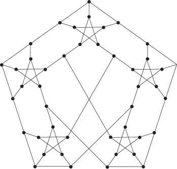
In the remainder of this section we describe the 31 snarks in detail and provide a computer-free proof that each of them has oddness at least $4$. Their adjacency lists, displayed in the order as they were generated, can be found in Appendix. Graph number 28 is illustrated in Figure 1, two more of the 31 graphs are depicted in Figure 1 and Figure 4 in our previous paper [8] which represent graphs number 15 and 17, respectively.

Figure 1: Graph number 28 of the 31 graphs in $\mathcal{M}$

Building blocks

The basic building blocks of all snarks constituting the set $\mathcal{M}$ are five multipoles $\mathbf{I}$, $\mathbf{H}_{1}$, $\mathbf{H}_{2}$, $\mathbf{T}$, and $\mathbf{N}$, described below, all of them arising from the Petersen graph by removing vertices or severing edges. Every individual member of $\mathcal{M}$ may have a small number of additional vertices not belonging to any of these subgraphs.

Figure 2: Building block $\mathbf{I}$

• Let $\mathbf{I}$ denote the $(2,2)$-pole arising from the Petersen graph by removing two adjacent vertices and grouping the semiedges formerly incident with the same vertex to the same connector; it is shown in Figure 2. Since every $3$-edge-colouring of $\mathbf{I}$ assigns the edges in the same connector the same colour, $\mathbf{I}$ is an is an isochromatic $4$-pole. It is the only isochromatic $4$-pole on eight vertices and at the same time the smallest connected isochromatic $4$-pole. In the symbolic representation of $\mathbf{I}$ we represent the edges in one of the connectors by bold lines, see Figure 6. This clearly determines the other connector as well. Due to the symmetry of the Petersen graph, the two connectors of $\mathbf{I}$ are interchangeable.

  We emphasise that the connectors of $\mathbf{I}$, as well as those of the other four building blocks $\mathbf{H}_{1}$, $\mathbf{H}_{2}$, $\mathbf{T}$, and $\mathbf{N}$, are unordered. Different orderings are needed for the construction of the members of $\mathcal{M}$, a fact which partially explains a relatively large size of this set.

  

  Figure 3: Building blocks $\mathbf{H}_{1}$ and $\mathbf{H}_{2}$

• Let $\mathbf{H}$ denote a $(2,2)$-pole formed from the Petersen graph by severing two independent edges and grouping the semiedges arising from the same edge to the same connector. Every $3$-edge-colouring of $\mathbf{H}$ assigns different colours to the dangling edges within the same connector, so $\mathbf{H}$ is a heterochromatic $4$-pole. There are two ways how to select a pair of independent edges in the Petersen graph – either at distance $1$ or at distance $2$. Accordingly, there exist two nonisomorphic heterochromatic $4$-poles on ten vertices, denoted by $\mathbf{H}_{1}$ and $\mathbf{H}_{2}$, respectively. Observe that there exists no bridgeless heterochromatic $4$-pole with fewer vertices. The two heterochromatic $4$-poles on ten vertices are displayed in Figure 3. In the symbolic representation of $\mathbf{H}$ we distinguish the two connectors of $\mathbf{H}$ again by using bold lines for one of the connectors, see Figure 6. Again, the connectors of both $\mathbf{H}_{1}$ and $\mathbf{H}_{2}$ are interchangeable.

  

  Figure 4: Building block $\mathbf{T}$

• Let $\mathbf{T}$ denote the $(2,3)$-pole obtained from the Petersen graph by removing an arbitrary vertex $v$ and severing an edge $e$ not incident with $v$; the semiedges formerly incident with $v$ are put to one connector and those arising by severing $e$ are put to the other connector. The resulting $(2,3)$-pole is shown in Figure 4. Given an arbitrary $3$-edge-colouring of $\mathbf{T}$, the edges of the $2$-connector receive two distinct colours $x$ and $y$, while the edges of the $3$-connector receive the colours $x+y$, $z$, $z$, where $z$ is any colour from $\{1,2,3\}$. In the symbolic representation of $\mathbf{T}$ the edges of the $2$-connector are drawn bold, see Figure 6.

  

  Figure 5: Building block $\mathbf{N}$

• Let $\mathbf{N}$ denote the $(2,2,1)$-pole arising from the Petersen graph by removing a path of length $2$. The two $2$-connectors consist of the edges formerly incident with the same end-vertex of the path, the $1$-connector gets the remaining edge. The resulting $(2,2,1)$-pole is shown in Figure 5. The important property of $\mathbf{N}$ consists in the fact that every $3$-edge-colouring of $\mathbf{N}$ assigns the edges of one of the $2$-connectors two distinct colours $x$ and $y$ while the edges of the other $2$-connector receive the same colour $z\in\{1,2,3\}$; the fifth edge of $\mathbf{N}$ is coloured $x+y$. In the symbolic representation of $\mathbf{N}$ the edges of one $2$-connector are drawn bold and the $1$-connector edge is drawn dashed, see Figure 6. As with $\mathbf{I}$ and $\mathbf{H}$ before, the two $2$-connectors of $\mathbf{N}$ are interchangeable.

Figure 6: Basic building blocks

Six classes

We divide the 31 snarks of $\mathcal{M}$ into six classes depending on the number of disjoint copies of $\mathbf{I}$, $\mathbf{H}$, $\mathbf{T}$, and $\mathbf{N}$, and on the number of additional vertices in the graph. For example, by $2\mathbf{H}+2\mathbf{I}+\mathbf{N}+1$ we denote the set of all snarks from $\mathcal{M}$ that consist of two copies of $\mathbf{H}$, which need not be isomorphic, two copies of $\mathbf{I}$, one copy of $\mathbf{N}$, and one additional vertex. We do not distinguish between the two varieties $\mathbf{H}_{1}$ and $\mathbf{H}_{2}$ of $\mathbf{H}$ because both of them play the same structural role within the snark in question and their contribution to increasing the oddness is the same. The six classes of $\mathcal{M}$ are

$$2\mathbf{H}+3\mathbf{I},\ 2\mathbf{H}+2\mathbf{I}+\mathbf{N}+1,\ \mathbf{H}+4\mathbf{I}+2,\ \mathbf{H}+3\mathbf{I}+\mathbf{T}+1,\ 5\mathbf{I}+4,\text{ and }\ 4\mathbf{I}+\mathbf{T}+3.$$

In the rest of this section we describe each of the classes in detail and prove that every member $G\in\mathcal{M}$ has $\omega(G)\geqslant 4$. In our discussion we will be employing certain standard combinations of the multipoles $\mathbf{I}$, $\mathbf{H}$, and $\mathbf{T}$ defined by means of junctions. The order of semiedges in connectors is in all cases irrelevant. We define the $(2,2)$-poles $\mathbf{Z}_{1}=\mathbf{I}\circ\mathbf{H}$ and $\mathbf{Z}_{2}=\mathbf{I}\circ\mathbf{H}\circ\mathbf{I}$, the $(2,3)$-pole $\mathbf{Z}_{4}=\mathbf{I}\circ\mathbf{T}$, where the junction involves the $2$-connector of $\mathbf{T}$, and the $(2,2,1)$-pole $\mathbf{Z}_{3}$ defined as follows: in the $(2,2)$-pole $\mathbf{I}\circ\mathbf{I}$ subdivide one of the edges between the two copies of $\mathbf{I}$ and subsequently attach a dangling edge to the new vertex of degree $2$; the connectors of $\mathbf{Z}_{3}$ are defined in the obvious way. The multipoles $\mathbf{Z}_{1}$, $\mathbf{Z}_{2}$, $\mathbf{Z}_{3}$, and $\mathbf{Z}_{4}$ are illustrated in Figure 7.

(a) dipole $\mathbf{Z}_{1}$

(b) Dipole $\mathbf{Z}_{2}$

(c) Dipole $\mathbf{Z}_{3}$

(d) Dipole $\mathbf{Z}_{4}$

Figure 7: Dipoles $\mathbf{Z}_{i}$

Lemma 3.

The following statements hold true:

$$\rho(\mathbf{Z}_{1})=\rho(\mathbf{Z}_{3})=\rho(\mathbf{Z}_{4})=1\ \text{ and }\ \rho(\mathbf{Z}_{2})=2.$$

Proof.

Observe that $\mathbf{Z}_{1}$ is uncolourable because it is a junction of an isochromatic $(2,2)$-pole $\mathbf{I}$ with a heterochromatic $(2,2)$-pole $\mathbf{H}$. Hence, $\rho(\mathbf{Z}_{1})\geqslant 1$. Similarly, every colouring of $\mathbf{T}$ assigns its $2$-connector two distinct colours while $\mathbf{I}$ is isochromatic, so $\mathbf{Z}_{4}=\mathbf{I}\circ\mathbf{T}$ is uncolourable too, and therefore $\rho(\mathbf{Z}_{4})\geqslant 1$ again. If the $(2,2,1)$-pole $\mathbf{Z}_{3}$ was colourable, then every $3$-edge-colouring of $\mathbf{Z}_{3}$ would assign the edges adjacent to the dangling edge of the $1$-connector two distinct colours. At most one of these colours would match the colour of the edge connecting the two copies of $\mathbf{I}$ in $\mathbf{Z}_{3}$. Therefore, the isochromatic property of at least one copy of $\mathbf{I}$ in $\mathbf{Z}_{3}$ would always be violated. Hence, $\mathbf{Z}_{3}$ is uncolourable, and therefore $\rho(\mathbf{Z}_{3})\geqslant 1$.

Finally we prove that $\rho(\mathbf{Z}_{2})\geqslant 2$. Since $\mathbf{Z}_{1}$ is contained in $\mathbf{Z}_{2}$ and $\rho(\mathbf{Z}_{1})\geqslant 1$, we infer that $\rho(\mathbf{Z}_{2})\geqslant 1$ as well. In particular, the graph $K$ obtained from $\mathbf{Z}_{2}$ by identifying the semiedges within each connector is a snark. To prove that $\rho(\mathbf{Z}_{2})\geqslant 2$ suppose to the contrary that $\rho(\mathbf{Z}_{2})=1$, and let $v$ be a vertex such that $\mathbf{Z}_{2}-v$ is $3$-edge-colourable. Clearly, $v$ cannot belong to a copy of $\mathbf{I}$ for otherwise $\mathbf{Z}_{2}-v$ would still contain a copy of $\mathbf{Z}_{1}$ and therefore would be uncolourable. Thus $v$ must belong to the copy of $\mathbf{H}$, and hence every $3$-edge-colouring of $\mathbf{Z}_{2}-v$ must assign the same colour to both semiedges in any of the connectors. Now we can match the semiedges of each connector, thereby obtaining a $3$-edge-colouring of $K-v$. Since $K$ is a snark, such a colouring does not exist. This contradiction proves that $\rho(\mathbf{Z}_{2})\geqslant 2$.

To establish the required equalities for each particular multipole one has to display the corresponding colourings. Finding such colourings is straightforward, and therefore is left to the reader. ∎

In our analysis of the $31$ snarks we will often need to distinguish between different copies of the same basic building block $\mathbf{B}\in\{\mathbf{I},\mathbf{H},\mathbf{T},\mathbf{N}\}$. For this purpose we will be using upper indices, for example $\mathbf{B}^{1}$, $\mathbf{B}^{2}$, etc.

Class 1: 2H + 3I  (7 graphs)

(a) Class 1a (3 graphs)

(b) Class 1b (4 graphs)

Figure 8: Class 1

This class splits into two subclasses, Class 1a and Class 1b, depending on how the building blocks are connected between each other. Both subclasses are illustrated in Figure 8. Each graph $G$ from Class 1 contains a copy of $\mathbf{Z}_{1}$ and a copy of $\mathbf{Z}_{2}$. Since the copies of $\mathbf{Z}_{1}$ and $\mathbf{Z}_{2}$ are disjoint, Lemma 3 implies that $\rho(G)\geqslant 3$ and hence $\omega(G)\geqslant 4$.

Class 1a consists of graphs 15, 17, and 18, while Class 1b contains graphs 1, 4, 21, and 24.

Class 2: 2H + 2I + N + 1  (4 graphs)

The structure of graphs from Class 2 is illustrated in Figure 9. It can be seen that every graph $G$ from Class 2 contains two disjoint copies of $\mathbf{Z}_{1}$, therefore $\rho(G)\geqslant 2$. Note each of the induced subgraphs $[\mathbf{H}^{1}\cup\mathbf{N}\cup\mathbf{H}^{2}]$, $[\mathbf{H}^{1}\cup\mathbf{I}^{1}]$, $[\mathbf{H}^{2}\cup\mathbf{I}^{2}]$, and $[\mathbf{I}^{1}\cup\mathbf{I}^{2}\cup\{v\}]$ is uncolourable, the last of them being isomorphic to $\mathbf{Z}_{3}$. Thus if there exist two vertices $u$ and $w$ in $G$ such that $G-\{u,w\}$ is colourable, then either one of them lies in $\mathbf{H}^{1}$ and the other lies in $\mathbf{I}^{2}$, or one of them lies in $\mathbf{H}^{2}$ and the other lies in $\mathbf{I}^{1}$. In all other cases one of the mentioned uncolourable subgraphs will remain intact. Without loss of generality we may assume that $u$ belongs to $\mathbf{H}^{1}$ and $w$ belongs $\mathbf{I}^{2}$. Since $\mathbf{I}^{1}$ is isochromatic, the edges between $\mathbf{I}^{1}$ and $\mathbf{H}^{1}$ have the same colour. Because $\mathbf{H}^{2}$ is heterochromatic, the colours the edges between $\mathbf{H}^{2}$ and $\mathbf{N}$ are different. The inverting property of $\mathbf{N}$ ensures that the edges between $\mathbf{N}$ and $\mathbf{H}^{1}$ also have the same colour. If we now identify the dangling edges within each connector of $\mathbf{H}^{1}$, we obtain a colouring of the Petersen graph with one vertex removed. This contradiction proves that that $\rho(G)>2$, which means that $\omega(G)\geqslant 4$, as required.

Class 2 contains graphs 10, 11, 19, and 27.

Figure 9: Class 2 (4 graphs)

Class 3: H + 4I + 2  (6 graphs)

(a) Class 3a (2 graphs)

(b) Class 3b (2 graphs)

(c) Class 3c (2 graphs)

Figure 10: Class 3

This class splits into three subclasses, 3a, 3b, and 3c. Their structure is represented in Figure 10. Every graph $G$ from Class 3a and Class 3b contains a copy of $\mathbf{Z}_{2}$ and a copy $\mathbf{Z}_{3}$, which are disjoint, therefore $\rho(G)\geqslant 3$ and $\omega(G)\geqslant 4$. Class 3c is somewhat different and requires a separate argument. Consider an arbitrary graph $G$ graph from Class 3c. Since $G$ contains a copy of $\mathbf{Z}_{1}$, we have $\rho(G)\geqslant 2$. Note that each of the subgraphs $[\mathbf{H}\cup\mathbf{I}^{1}]$, $[\mathbf{I}^{2}\cup\mathbf{I}^{3}\cup\{x\}]$, and $[\mathbf{I}^{3}\cup\mathbf{I}^{4}\cup\{y\}]$ has resistance 1. Thus if there exist two vertices $u$ and $w$ in $G$ such that $G-\{u,w\}$ is $3$-edge-colourable, then one of them, say $u$, lies in $[\mathbf{H}\cup\mathbf{I}^{1}]$ and the other belongs to $\mathbf{I}^{3}$. Since $\mathbf{I}^{2}$ and $\mathbf{I}^{4}$ remain intact in $G-\{u,w\}$, the isochromatic property of $\mathbf{I}$ implies that the edge $e$ connecting $\mathbf{I}^{2}$ to $\mathbf{H}$ has the same colour as the edge $f$ connecting $\mathbf{I}^{4}$ to $\mathbf{H}$. Since $\mathbf{H}$ is heterochromatic, we conclude that $u$ lies in $\mathbf{H}$. As a consequence, $\mathbf{I}^{1}$ remains intact in $G-\{u,w\}$ too, which means that the two edges $e^{\prime}$ and $f^{\prime}$ joining $\mathbf{H}$ to $\mathbf{I}^{1}$ are equally coloured as well. But then the induced colouring of $\mathbf{H}$ yields a $3$-edge-colouring of the Petersen graph with a single vertex removed. This contradiction proves that $\rho(G)>2$ and $\omega(G)\geqslant 4$.

Class 3a contains graphs 5 and 6, Class 3b contains graphs 7 and 23, and Class 3c contains graphs 9 and 26.

Class 4: H + 3I + T + 1  (10 graphs)

(a) Class 4a (4 graphs)

(b) Class 4b (6 graphs)

Figure 11: Class 4

Class 4 has two subclasses 4a and 4b, both shown in Figure 11. Every graph $G$ from Class 4 contains disjoint copies of $\mathbf{Z}_{2}$ and $\mathbf{Z}_{4}$, so $\rho(G)\geqslant 3$ and $\omega\geqslant 4$.

Class 4a consists of graphs 2, 3, 13, and 14, and Class 4b contains graphs 8, 12, 16, 20, 22, and 25.

(a) Class 5a (1 graph)

(b) Class 5b (1 graph)

Figure 12: Class 5

Class 5: 5I + 4  (2 graphs)

Class 5 has two subclasses Class 5a and Class 5b; they are represented in Figure 12. Observe that every member of Class 5 contains a $5$-pole isomorphic to $\mathbf{Z}_{3}$, namely $[\mathbf{I}^{1}\cup\mathbf{I}^{2}\cup\{v_{1}\}]$, whose resistance is 1 by Lemma 3. Hence, every member of Class 5 is indeed a snark.

Now, let us consider a graph $G$ from Class 5a. To prove that $\omega(G)\geqslant 4$ suppose the contrary. Then $\omega(G)=\rho(G)=2$, which means that there exist vertices $u$ and $w$ in $G$ such that $G-\{u,w\}$ is colourable. Since each of the $5$-poles $[\mathbf{I}^{k}\cup\mathbf{I}^{k+1}\cup\{v_{k}\}]$, with $k\in\{1,2,3,4\}$, is isomorphic to $\mathbf{Z}_{3}$, and $\rho(\mathbf{Z}_{3})=1$, none of them survives in $G-\{u,w\}$. It follows that one of $u$ and $w$ lies in $\mathbf{I}^{2}$ and the other one lies in $\mathbf{I}^{4}$. Let $\varphi$ be a $3$-edge-colouring of $G-\{u,w\}$. Without loss of generality we may assume that $\varphi(f_{1})=1$, $\varphi(g_{1})=2$ and $\varphi(h_{1})=3$. Since $\mathbf{I}^{1}$ remains intact in $G-\{u,w\}$, we have $\varphi(e_{1})=1$. Similarly, since $\mathbf{I}^{5}$ is intact, we have $\varphi(h_{2})=\varphi(h_{1})=3$. Consider the colours of $e_{2}$ and $f_{2}$. Since $\mathbf{I}^{3}$ remains intact $G-\{u,w\}$, we deduce that $\varphi(e_{2})=\varphi(g_{2})$ and hence $\varphi(e_{2})\neq\varphi(f_{2})$. Furthermore, $\{1,2\}=\{\varphi(e_{1}),\varphi(g_{1})\}\neq\{\varphi(e_{2}),\varphi(f_{2})\}$ because otherwise the induced colouring of $\mathbf{I}^{2}$ would give rise to a $3$-edge-colouring of the Petersen graph with one vertex removed, which is impossible. Therefore $\{\varphi(e_{2}),\varphi(f_{2})\}=\{1,3\}$ or $\{2,3\}$, but since $\varphi(f_{2})\neq\varphi(h_{2})=3$ we conclude that $\varphi(e_{2})=3$. However, the isochromatic property of $\mathbf{I}^{3}$ forces $\varphi(g_{2})=\varphi(e_{2})=3$, which is in conflict with the value $\varphi(h_{2})=3$ because $g_{2}$ and $h_{2}$ are adjacent. Therefore $\rho(G)\geqslant 3$ and $\omega(G)\geqslant 4$.

Next, let us consider a graph $G$ from Class 5b. We wish to prove that $\omega(G)\geqslant 4$. Suppose the contrary. Then $\rho(G)=2$, which again means that there exist vertices $u$ and $w$ in $G$ such that $G-\{u,w\}$ is $3$-edge-colourable. In this case it is easy to see that one of the vertices belongs $\mathbf{I}^{2}$ and the other one belongs to $\mathbf{I}^{4}\cup\mathbf{I}^{5}\cup\{v_{4}\}$. Suppose that the vertex $w$ lies in $\mathbf{I}^{5}\cup\{v_{4}\}$ so that $\mathbf{I}^{4}$ remains intact. Take an arbitrary $3$-edge-colouring $\varphi$ of $G-\{u,w\}$, and let $\varphi(f_{3})=x$. Since $\mathbf{I}^{1}$ and $\mathbf{I}^{3}$ are also left intact in $G-\{u,w\}$, we deduce that $\varphi(e_{3})=x$, $\varphi(g_{2})=x$, and finally $\varphi(g_{1})=x$. However, the edges $g_{1}$ and $e_{3}$ are adjacent, so this is impossible. Therefore $w\in\mathbf{I}^{4}$, which means that $\mathbf{I}^{5}$ is left intact. In this situation we can derive a contradiction in a similar way as for Class 5a. This proves that $\omega(G)\geqslant 4$ for every graph from Class 5b.

Both Class 5a and Class 5b consist of a single graph each – graphs 28 and 30, respectively.

Figure 13: Class 6 (2 graphs)

Class 6: 4I + T + 3  (2 graphs)

The structure of Class 6 is displayed in Figure 13. Let us first observe that every member $G$ of Class 6 is uncolourable because it contains the subgraph $[\mathbf{I}^{1}\cup\mathbf{T}]$ isomorphic to $\mathbf{Z}_{4}$, whose resistance equals 1 by Lemma 3. It follows that $\rho(G)\geqslant 2$. To prove that $\omega(G)\geqslant 4$ suppose to the contrary that $\omega(G)=2=\rho(G)$. Since each of the subgraphs $[\mathbf{I}^{k}\cup\mathbf{I}^{k+1}\cup\{v_{k}\}]$, with $k\in\{2,3\}$, is also uncolourable, there exist vertices $u\in\mathbf{I}^{3}$ and $w\in[\mathbf{I}^{1}\cup\mathbf{T}]$ such that $G-\{u,w\}$ is $3$-edge-colourable. Let $\varphi$ be one such colouring. Without loss of generality we may assume that $\varphi(e_{1})=1$, $\varphi(e_{2})=2$, and $\varphi(e_{3})=3$. Since $\mathbf{I}^{2}$ and $\mathbf{I}^{4}$ are left intact, we have $\varphi(f_{1})=2$ and $\varphi(f_{2})=3$. Put together, the edges of the $3$-connector of $\mathbf{T}$ receive three distinct colours from the colouring $\varphi$. As previously mentioned, every $3$-edge-colouring of $\mathbf{T}$ forces a repeated colour in the $3$-connector. Therefore $w$ must belong to $\mathbf{T}$. It follows that $\mathbf{I}^{1}$ remains intact and therefore $\varphi(g_{1})=\varphi(g_{2})$. But then the induced colouring of $\mathbf{T}$ yields a $3$-edge-colouring of the Petersen graph with a single vertex removed. This contradiction proves that $\omega(G)\geqslant 4$.

Class 6 contains two nonisomorphic graphs – 29 and 31.

Properties of graphs in $\mathcal{M}$

We have determined the values of several invariants for the 31 snarks in $\mathcal{M}$. In most cases the computations were performed by a computer. The evaluated invariants can be divided into two groups. The first group is constituted by general invariants: namely, the order of the automorphism group, genus (minimum genus of an orientable surface upon which a given graph can be drawn without intersections), diameter, radius, and circumference (the maximal circuit length in a graph). The values of these invariants for individual members of $\mathcal{M}$ are summarised in Table 1. In particular, all members of $\mathcal{M}$ have circumference $41$, that is, $n-3$ where $n$ is the number of vertices. The values of the remaining invariants vary over the set $\mathcal{M}$. It is quite remarkable that the automorphism group of every graph in $\mathcal{M}$ is a $2$-group (or is trivial).

Class	Graph number	$|{\rm Aut}(G)|$	Genus	Diameter	Radius	Circumference
1a	15	4	4	8	6	41
1a	17	64	5	8	7	41
1a	18	8	5	8	7	41
1b	1	16	5	8	6	41
1b	4	1	4	8	6	41
1b	21	4	5	8	6	41
1b	24	4	5	8	6	41
2	10	2	4	8	5	41
2	11	2	4	8	5	41
2	19	16	5	8	5	41
2	27	2	5	8	5	41
3a	5	4	5	8	6	41
3a	6	1	4	8	6	41
3b	7	2	5	8	6	41
3b	23	8	5	8	6	41
3c	9	4	4	8	6	41
3c	26	1	4	8	6	41
4a	2	8	5	8	7	41
4a	3	4	5	8	7	41
4a	13	2	4	8	6	41
4a	14	1	4	8	6	41
4b	8	1	4	8	6	41
4b	12	1	4	8	6	41
4b	16	4	5	8	6	41
4b	20	1	5	8	6	41
4b	22	4	5	8	6	41
4b	25	4	5	8	6	41
5a	28	2	4	8	6	41
5b	30	2	5	7	6	41
6	29	2	5	7	6	41
6	31	1	4	8	6	41

Table 1: Basic invariant values for the 31 snarks of $\mathcal{M}$.

The second group of invariants comprises those which are of particular interest for snarks: perfect matching index $\pi$, resistance $\rho$, weak oddness $\omega^{\prime}$, and two invariants introduced in [15, 26, 27] and denoted by $\mu_{3}$ and $\gamma_{2}$; see also [5] for a recent survey. The perfect matching index of a bridgeless cubic graph $G$, denoted by $\pi(G)$ (also known as excessive index and denoted by $\chi^{\prime}_{e}$), is the smallest number of perfect matchings that cover all the edges of $G$ [2, 7]. The weak oddness of a cubic graph $G$, denoted by $\omega^{\prime}(G)$, is the smallest number of components of odd order in an even factor of $G$; by an even factor we mean a spanning subgraph with all degrees even. Given a bridgeless cubic graph $G$, we define $\gamma_{2}(G)$ to be the smallest number of common edges that two perfect matchings of $G$ can have, and let $\mu_{3}(G)$ be the smallest number of edges of $G$ that are left uncovered by the union of any three perfect matchings of $G$.

The perfect matching index $\pi(G)$ of $G$ is bounded below by $3$ and equals $3$ if and only if $G$ is $3$-edge-colourable. It is believed, by a conjecture of Berge (see [23]), that $\pi(G)\leqslant 5$ for every bridgeless cubic graph $G$. This conjecture, if true, thus divides all snarks into two subclasses, those with perfect matching index equal to $4$, and those with perfect matching index $5$. We have determined that $\pi(G)=4$ for every $G\in\mathcal{M}$.

The remaining invariants, along with oddness, can be regarded as measures of uncolourability as they take value $0$ on $3$-edge-colourable graphs, and positive values otherwise. Their comparison with oddness and resistance may therefore be very instructive.

First of all, using a computer we have determined that $\rho(G)=3$ for all snarks $G\in\mathcal{M}$. As regards weak oddness, it is easy to see that $\omega^{\prime}(G)$ is an even integer such that $\rho(G)\leqslant\omega^{\prime}(G)\leqslant\omega(G)$. Furthermore, if $\omega(G)=4$, then necessarily $\omega^{\prime}(G)=4$ as well, because otherwise $\omega^{\prime}(G)=2$ would immediately yield $\rho(G)=2$ whence $\omega(G)=2$. In particular, for all snarks $G\in\mathcal{M}$ we have $\omega^{\prime}(G)=\omega(G)=4$. It is known, however, that in general both the difference $\omega(G)-\omega^{\prime}(G)$ and $\omega^{\prime}(G)-\rho(G)$ can be arbitrarily large (see [1, 17]).

We finish this section by discussing the previously mentioned invariants $\gamma_{2}$ and $\mu_{3}$. In [27, Proposition 2.1] Steffen proved that $\omega(G)\leqslant 2\gamma_{2}(G)$ for every bridgeless cubic graph $G$. Using a computer we have determined that $\gamma_{2}(G)=2$ for every $G\in\mathcal{M}$, which shows that every snark from $\mathcal{M}$ fulfils the upper bound on $\omega$ set by $\gamma_{2}$ with equality. Similarly, in [15, Corollary 2.4] Jin and Steffen proved that $\omega(G)\leqslant 2\mu_{3}(G)/3$ for every bridgeless cubic graph. Using a computer we have determined that all snarks $G\in\mathcal{M}$ have $\mu_{3}(G)=6$, which means that they again reach the upper bound on $\omega$ in terms of $\mu_{3}$ with equality. Snarks with the latter property have a very special structure of sets of edges left uncovered by three perfect matchings and therefore deserve special attention.

The values of perfect matching index, resistance, weak oddness, $\gamma_{2}$, and $\mu_{3}$ for the snarks of $\mathcal{M}$ are summarised in Table 2.

$\pi$	$\rho$	$\omega^{\prime}$	$\gamma_{2}$	$\mu_{3}$
4	3	4	2	6

Table 2: Values of perfect matching index and unclourability measures for the snarks of $\mathcal{M}$

Infinite families

Each of the six classes described above gives rise to an infinite family of snarks with oddness at least $4$ and cyclic connectivity $4$. It is sufficient to replace the basic building blocks $\mathbf{I}$, $\mathbf{H}$, $\mathbf{T}$, and $\mathbf{N}$ obtained from the Petersen graph with similar structures created from any cyclically $4$-edge-connected snark. With a little additional care one can construct infinite families of snarks with increasing oddness.

4 Completeness of $\mathcal{M}$

In this section we prove that the set $\mathcal{M}$, constructed and analysed in Section 3, is the complete set of pairwise nonisomorphic snarks with cyclic connectivity $4$, oddness at least $4$, and minimum order. Our point of departure is the following theorem proved in [8].

Theorem 4.

The smallest number of vertices of a snark with cyclic connectivity $4$ and oddness at least $4$ is $44$. The girth of each such snark is at least $5$.

This result is a consequence of the following stronger and more detailed result from [8] which will be needed for the proof of the main result of this paper.

Theorem 5.

Let $G$ be a snark with oddness at least $4$, cyclic connectivity $4$, and minimum number of vertices. Let $S$ be a cycle-separating $4$-edge-cut in $G$ whose removal leaves components $G_{1}$ and $G_{2}$. Then, up to permutation of the index set $\{1,2\}$, exactly one of the following occurs.

• Both $G_{1}$ and $G_{2}$ are uncolourable, in which case each of them can be extended to a cyclically $4$-edge-connected snark by adding two vertices.

• $G_{1}$ is uncolourable and $G_{2}$ is heterochromatic, in which case $G_{1}$ can be extended to a cyclically $4$-edge-connected snark by adding two vertices, and $G_{2}$ can be extended to a cyclically $4$-edge-connected snark by adding two isolated edges.

• $G_{1}$ is uncolourable and $G_{2}$ is isochromatic, in which case $G_{1}$ can be extended to a cyclically $4$-edge-connected snark by adding two vertices, and $G_{2}$ can be extended to a cyclically $4$-edge-connected snark by adding two vertices, except possibly $\zeta(G_{2})=2$. In the latter case, $G_{2}$ is a partial junction of two colour-open $4$-poles, which may be isochromatic or heterochromatic in any combination.

Here is our main result:

Theorem 6.

The set $\mathcal{M}$ is the complete set of snarks with cyclic connectivity $4$ and oddness at least $4$ on $44$ vertices.

Let $\mathcal{N}$ be the set of all snarks with cyclic connectivity $4$ and oddness at least $4$ on $44$ vertices. To prove Theorem 6 it suffices to show that $\mathcal{N}\subseteq\mathcal{M}$. The general strategy of the proof is to show that every snark $G\in\mathcal{N}$ is a $4$-join of two cyclically $4$-edge-connected snarks of order at most 36. As soon as this is done, one can perform $4$-joins in all possible ways that give rise to a cyclically $4$-edge-connected snark of order $44$, identify those whose oddness equals $4$, and check whether all of them belong to $\mathcal{M}$.

In order to apply this strategy we employ Theorem 5. It implies that we can split each $G\in\mathcal{N}$ into two subgraphs $G_{1}$ and $G_{2}$ each of which can be extended to cyclically a $4$-edge-connected snark by adding at most two vertices. The difficult part of the proof arises when one of the subgraphs, namely $G_{1}$, has 36 vertices and $G_{2}$ is an isochromatic $4$-pole on $8$ vertices (see (iii) of Theorem 5). Adding two adjacent vertices to $G_{1}$ is now useless because the list of all cyclically $4$-edge-connected snarks is known only up to 36 vertices [4, 8]. Instead, we show that it is possible to add two isolated edges to $G_{1}$ in such a way that a cyclically $4$-edge-connected snark of order 36 is created. A detailed analysis that precedes this step is the core of the proof of Theorem 6, which now follows.

Proof.

Let $G$ be a snark with cyclic connectivity 4 and oddness at least 4 on 44 vertices. We wish to prove that $G\in\mathcal{M}$. Suppose the contrary. In order to derive a contradiction we first establish four claims.

Claim 1. Every cycle-separating $4$-edge-cut of $G$ determines two components, one uncolourable on $36$ and one isochromatic on $8$ vertices. Both components are $2$-edge-connected.

Proof of Claim 1. Let $S$ be an arbitrary cycle-separating $4$-edge-cut in $G$ and let $G_{1}$ and $G_{2}$ be the components of $G-S$. Since $S$ is a minimum cycle-separating edge-cut, both $G_{1}$ and $G_{2}$ are easily seen to be $2$-edge-connected. ¿From Theorem 5 we deduce that one of the components, say $G_{1}$, is uncolourable. If $G_{2}$ was either uncolourable or heterochromatic, then it would have at least 10 vertices and hence $G_{1}$ has at most $34$ vertices. Using Theorem 5 again we could conclude that both $G_{1}$ and $G_{2}$ can be extended to snarks of order at most $36$, so $G$ would be a $4$-join of two snarks from $\mathcal{S}_{36}$ and therefore a member of $\mathcal{M}$. This contradiction shows that $G_{2}$ is isochromatic.

Now we prove that the isochromatic component produced by an arbitrary cycle-separating $4$-edge-cut has only eight vertices. Suppose to the contrary that there exists a cycle separating edge-cut $R$ in $G$ such that the isochromatic component, denoted by $J$, has at least ten vertices. Choose $R$ to minimise the number of vertices of $J$. Clearly, the other component $K$ of $G-R$ has at most $34$ vertices and, by the first part of the proof, it is uncolourable. It follows that $K$ also has at least ten vertices, so $J$ has at most $34$ vertices too. Theorem 5 further implies that $K$ can be extended to a cyclically $4$-edge-connected snark $\tilde{K}$ by adding two vertices. If $\zeta(J)\geqslant 3$, the same theorem implies that $J$ can also be extended to a cyclically $4$-edge-connected snark $\tilde{J}$ by adding two vertices. Since both $\tilde{J}$ and $\tilde{K}$ have order at most 36, $G$ belongs to $\mathcal{M}$ – a contradiction. Therefore $J$ has a $2$-edge-cut. By Theorem 5 (iii), $J$ is a partial junction of two colour-open $4$-poles $J_{1}$ and $J_{2}$. Since both $\delta_{G}(J_{1})$ and $\delta_{G}(J_{2})$ are cycle-separating $4$-edge-cuts, both $J_{1}$ and $J_{2}$ must be isochromatic. If any of them had more than eight vertices, then the corresponding edge-cut would contradict the choice of $R$. Therefore $J$ is a partial junction of two copies of the isochromatic $4$-pole $\mathbf{I}$ on eight vertices, so $J$ has 16 vertices and $K$ has 28 vertices. It follows that $G$ can be expressed in the form $(P\odot P)\otimes H$ where $P$ is the Petersen graph, $H$ is a snark on 30 vertices, and $L_{1}\odot L_{2}$ denotes a $4$-join of cubic graphs $L_{1}$ and $L_{2}$ which employs $4$-poles resulting from the removal of two adjacent vertices from both $L_{1}$ and $L_{2}$, while $Q_{1}\otimes Q_{2}$ denotes a $4$-join of cubic graphs $Q_{1}$ and $Q_{2}$ which employs a $4$-pole obtained from $Q_{1}$ by removing two nonadjacent edges and a $4$-pole obtained from $Q_{2}$ by removing two adjacent vertices. Using a computer we have constructed all graphs $G$ arising in this way and verified that each of them either belongs to $\mathcal{M}$ or has oddness at most $2$. This contradiction establishes Claim 1.

Claim 2. Every $4$-edge-cut in $G$ separates a subgraph with at most eight vertices from the rest of $G$.

Proof of Claim 2. Let $Q$ be a $4$-edge-cut in $G$. If one of the components of $G-Q$ is acyclic, then, by Lemma 1, this component has two vertices. If $Q$ is cycle-separating, then the conclusion follows from Claim 1. Claim 2 is proved.

Fix a cycle-separating $4$-edge-cut $S$ in $G$; we will refer to $S$ as the principal $4$-edge-cut of $G$. As before, let $G_{1}$ and $G_{2}$ be the components of $G-S$ where $G_{1}$ is uncolourable. By Claim 1, the other component $G_{2}$ is isochromatic on eight vertices. Let $A$ be the set of end-vertices of $S$ in $G_{1}$. Since $S$ is independent, we have $|A|=4$.

The remainder of the proof is devoted to proving the following fact:

• The component $G_{1}$ can be extended to a cyclically $4$-edge-connected snark by adding two edges between the vertices of $A$.

As a consequence, $G$ will be a $4$-join of two graphs from $\mathcal{S}_{36}$, and therefore a member of $\mathcal{M}$. This will provide a final contradiction.

Claim 3.$G_{1}$ is cyclically $3$-edge-connected and has a cycle-separating $3$-edge-cut.

Proof of Claim 3. If $\zeta(G_{1})\geqslant 4$, then adding to $G_{1}$ two edges joining the vertices of $A$ in an arbitrary manner would produce a cyclically $4$-edge-connected snark of order 36. Consequently, $G$ would belong to $\mathcal{M}$. Therefore $\zeta(G_{1})\leqslant 3$. To prove that $\zeta(G_{1})\geqslant 3$ suppose to the contrary that $G_{1}$ has a cycle-separating 2-edge-cut $U$, and let $G_{11}$ and $G_{12}$ be the two components of $G_{1}-U$. Since $G$ is cyclically $4$-edge-connected, two edges of $S$ join $G_{2}$ to $G_{11}$ and other two edges of $S$ join $G_{2}$ to $G_{12}$. Thus $\delta_{G}(G_{11})$ is a cycle-separating $4$-edge-cut which separates $G_{11}$ from $G_{12}\cup G_{2}$. Since $G_{12}\cup G_{2}$ contains more then eight vertices, Claim 1 implies that $G_{11}$ is an isochromatic dipole on eight vertices. Likewise, $G_{12}$ is an isochromatic dipole on eight vertices. Put together, $G$ has altogether $24$ vertices, which is again a contradiction. Therefore $\zeta(G_{1})=3$. Finally, $G_{1}$ is homeomorphic to a certain cubic graph $\bar{G}_{1}$ with $\zeta(\bar{G}_{1})=\zeta(G_{1})$ on 32 vertices, so $G_{1}$ is not a subdivision of the complete graph $K_{4}$ and therefore contains a cycle-separating $3$-edge-cut. This establishes Claim 3.

Before we can proceed we need two definitions. First, a cycle-separating $3$-edge-cut $Q$ in $G_{1}$ will be called balanced if each component of $G_{1}-Q$ is incident with exactly two edges of the principal $4$-edge-cut $S$. Otherwise, $Q$ will be called unbalanced. Second, let $R$ and $T$ be two cycle-separating $3$-edge-cuts in $G_{1}$. Let $X_{1}$ and $X_{2}$ be the components of $G_{1}-R$ and let $Y_{1}$ and $Y_{2}$ be the components of $G_{1}-T$. The edge-cuts $R$ and $T$ in $G_{1}$ will be called comparable if $X_{i}\subseteq Y_{j}$ or $Y_{j}\subseteq X_{i}$ for some $i,j\in\{1,2\}$.

Claim 4. $G_{1}$ contains two incomparable balanced $3$-edge-cuts.

Proof of Claim 4. Let us first observe that if $Q$ is an arbitrary unbalanced $3$-edge-cut in $G_{1}$, then adding any two edges between the vertices of $A$ in an arbitrary manner will produce a cubic graph $\tilde{G}_{1}$ where $Q$ has ceased to be an edge-cut. It follows that if every cycle-separating $3$-edge-cut in $G_{1}$ is unbalanced, then $\tilde{G}_{1}$ is a cyclically $4$-edge-connected snark and $G$ is a $4$-join of $\tilde{G}_{1}$ with the Petersen graph. Since $G_{1}$ has $36$ vertices, $G\in\mathcal{M}$ and we have arrived at a contradiction. Therefore $G_{1}$ must contain a balanced $3$-edge-cut.

Figure 14: Comparable balanced $3$-edge-cuts

If every pair of balanced $3$-edge-cuts in $G_{1}$ is comparable, we can arrange the balanced $3$-edge-cuts in an increasing linear order, say $Q_{1},\ldots,Q_{m}$. Clearly, there is a component $H_{1}$ of $G_{1}-Q_{1}$ and a component $H_{m}$ of $G_{1}-Q_{m}$ such that both of them are disjoint from all of $Q_{1},\ldots,Q_{m}$. It is easy to see that $H_{1}$ contains two vertices of $A$ while $H_{m}$ contains the other two, see Figure 14. Thus we can connect the two vertices of $H_{1}\cap A$ to those of $H_{m}\cap A$ by two edges, producing a cyclically $4$-edge-connected snark $\tilde{G}_{1}$. Again, $G$ is a $4$-join of $\tilde{G}_{1}$ with the Petersen graph, so $G$ belongs to $\mathcal{M}$ contrary to the assumption. Therefore $G_{1}$ contains two incomparable balanced $3$-edge-cuts. This proves Claim 4.

Figure 15: Crossing edge-cuts $R$ and $T$

In the rest the proof we explore the structure of $G_{1}$ arising from a pair of incomparable balanced $3$-edge-cuts. Let $R$ and $T$ be any two incomparable balanced 3-edge-cuts in $G_{1}$. Clearly, $G_{1}-R$ has two components, say $X_{1}$ and $X_{2}$, and $G_{1}-T$ has two components, say $Y_{1}$ and $Y_{2}$. The definition of comparable edge-cuts readily implies that each of the subgraphs $X_{i}\cap Y_{j}$ is non-empty. Let $a$ be the number of edges between $X_{1}\cap Y_{1}$ and $X_{1}\cap Y_{2}$, $b$ the number of edges between $X_{1}\cap Y_{1}$ and $X_{2}\cap Y_{2}$, $c$ the number of edges between $X_{1}\cap Y_{1}$ and $X_{2}\cap Y_{1}$, $d$ the number of edges between $X_{1}\cap Y_{2}$ and $X_{2}\cap Y_{1}$, $e$ the number of edges between $X_{2}\cap Y_{1}$ to $X_{2}\cap Y_{2}$, and finally $f$ the number of edges between $X_{1}\cap Y_{2}$ and $X_{2}\cap Y_{2}$; see Figure 15.

Since $X_{1}$, $X_{2}$, $Y_{1}$ and $Y_{2}$ are all connected, we have

$$a\geqslant 1,\quad e\geqslant 1,\quad c\geqslant 1,\quad f\geqslant 1.$$ (1)

Next,

$$|R|=|\delta_{G_{1}}(X_{1})|=c+f+b+d=3$$ (2)

and

$$|T|=|\delta_{G_{1}}(Y_{1})|=a+e+b+d=3.$$ (3)

By combining (1) and (2) we can further conclude that

$$b+d\leqslant 1.$$ (4)

We now consider two cases according to whether there exists a set $X_{i}\cap Y_{j}$ such that $X_{i}\cap X_{j}\cap A=\emptyset$ or not.

Case 1: There exists a subgraph $X_{i}\cap Y_{j}$, with $i,j\in\{1,2\}$, such that $X_{i}\cap X_{j}\cap A=\emptyset$. In view of symmetry we can clearly assume that $X_{1}\cap X_{2}\cap A=\emptyset$. In this situation $X_{1}\cap Y_{2}$ is incident with two edges of $S$, because $R$ is balanced, and $X_{2}\cap Y_{1}$ is incident with the other two edges of $S$, because $T$ is balanced. It follows that $|X_{2}\cap Y_{2}\cap A|=0$ as well.

With (1) in mind, we first prove that $a=e=c=f=1$. Suppose to the contrary that one of these values is strictly greater than $1$. In view of symmetry we can assume that $a>1$. Now (1) and (3) forces $a=2$, $e=1$, $b=0$, and $d=0$, which together with (2) implies that either $c=2$ and $f=1$, or $c=1$ and $f=2$. In the former case, $|\delta_{G}(X_{2}\cap Y_{2})|=b+e+f=2$ contrary to the fact that $G$ is $3$-edge-connected, while in the latter case $X_{2}\cap Y_{1}$ is separated from the rest of $G_{1}$ by $c+d+e=2$ edges, contradicting Claim 3. Therefore $a=e=c=f=1$.

Now, (2) and (4) imply that $b+d=1$. However, $b\geqslant 1$ for otherwise $|\delta_{G}(X_{1}\cap Y_{1})|=a+b+c=2$, contrary to the fact that $G$ is $3$-edge-connected. So $b=1$ and $d=0$. It follows that $|\delta_{G}(X_{1}\cap Y_{1})|=a+b+c=3$ and $|\delta_{G}(X_{2}\cap Y_{2})|=b+e+f=3$. Since $G$ is cyclically $4$-edge-connected, both $X_{1}\cap Y_{1}$ and $X_{2}\cap Y_{2}$ are acyclic, and therefore, by Lemma 1, both consist of a single vertex. Further, $|\delta_{G}(X_{1}\cap Y_{2})|=2+a+d+f=4$ and $|\delta_{G}(X_{2}\cap Y_{1})|=2+c+d+e=4$, so $|X_{1}\cap Y_{2}|\geqslant 2$ and $|X_{2}\cap Y_{1}|\geqslant 2$. By Claim 2, one of the components determined by $\delta_{G}(X_{1}\cap Y_{2})$ has at most eight vertices. Since the number of vertices of $G$ lying outside $X_{1}\cap Y_{2}$ is

$$|G_{2}|+|X_{2}\cap Y_{1}|+|X_{1}\cap Y_{1}|+|X_{2}\cap Y_{2}|\geqslant 8+2+1+1=12,$$

we conclude that $|X_{1}\cap Y_{2}|\leqslant 8$. Similarly, $|X_{2}\cap Y_{1}|\leqslant 8$. Summing up,

$$|G_{1}|\leqslant|X_{1}\cap Y_{1}|+|X_{2}\cap Y_{2}|+|X_{1}\cap Y_{2}|+|X_{2}\cap Y_{1}|\leqslant 1+1+8+8<36,$$

which contradicts Claim 1. This establishes Case 1.

Case 2: $X_{i}\cap X_{j}\cap A\neq\emptyset$ for each $i,j\in\{1,2\}$. Clearly, this is only possible when each of the subgraphs $X_{i}\cap Y_{i}$ is incident with exactly one edge of the principal $4$-edge-cut $S$. We may assume that $A=\{a_{1},a_{2},a_{3},a_{4}\}$ where $a_{1}$ lies in $X_{1}\cap Y_{1}$, $a_{2}$ lies in $X_{1}\cap Y_{2}$, $a_{3}$ lies in $X_{2}\cap Y_{1}$, and $a_{4}$ lies in $X_{2}\cap Y_{2}$.

For each $X_{i}\cap Y_{i}$ we count the number of edges of $R\cup T$ this subgraph is incident with. According to (1) we obtain

$$a+b+c\geqslant 2,\quad a+d+f\geqslant 2,\quad c+d+e\geqslant 2,\quad b+e+f\geqslant 2.$$ (5)

If all the inequalities in (5) are strict, then summing the first two of them yields

$$6\leqslant 2a+(b+c+d+f)=2a+|R|=2a+3,$$

whence $a\geqslant 2$. Similarly, summing the latter two inequalities implies that $e\geqslant 2$. But then

$$|T|=a+b+d+e\geqslant 4,$$

which is a contradiction.

Therefore at least one of the inequalities in (5) holds with equality. Due to symmetry we may assume that $a+b+c=2$. From (1) we now infer that $a=c=1$ and $b=0$. If we plug these values into (2) and (3), we get $d+f=2=d+e$. Since $d\leqslant 1$ on account of (4), we conclude that either $d=e=f=1$, or $d=0$ and $e=f=2$.

First assume that $d=e=f=1$. In this case $|\delta_{G}(X_{1}\cap Y_{1})|=3=|\delta_{G}(X_{2}\cap Y_{2})|$, so $|X_{1}\cap Y_{1}|=1=|X_{2}\cap Y_{2}|$ by Lemma 1. Furthermore, $|\delta_{G}(X_{1}\cap Y_{2})|=|\delta_{G}(X_{2}\cap Y_{1})|=4$. By Claim 2, one of the components determined by $\delta_{G}(X_{1}\cap Y_{2})$ has at most eight vertices. As in Case 1, the number of vertices of $G$ outside $X_{1}\cap Y_{2}$ is at least $12$, so $|X_{1}\cap Y_{2}|\leqslant 8$. Similarly $|X_{2}\cap Y_{1}|\leqslant 8$, and therefore $|G_{1}|\leqslant 1+1+8+8<36$, which contradicts Claim 1.

Next assume that $d=0$ and $e=f=2$. Recall that $a=c=1$ and $b=0$. It follows that $|\delta_{G}(X_{1}\cap Y_{1})|=3$ which means that $X_{1}\cap X_{1}$ consists of a single vertex $a_{1}$. Further, $|\delta_{G}(X_{1}\cap Y_{2})|=4$ and $|\delta_{G}(X_{2}\cap Y_{1})|=4$, so $|X_{1}\cap Y_{2}|\leqslant 8$ and $|X_{2}\cap Y_{1}|\leqslant 8$. Also, $|\delta_{G}(X_{2}\cap Y_{2})|=5$. In fact, Claim 1 implies that $X_{1}\cap Y_{2}$ and $X_{2}\cap Y_{1}$ are isochromatic $4$-poles on eight vertices, because $R$ and $T$ are cycle-separating edge-cuts and hence $X_{1}\cap Y_{2}$ and $X_{2}\cap Y_{1}$ must contain circuits.

We show that $X_{2}\cap Y_{2}$ is $2$-edge-connected. If $X_{2}\cap Y_{2}$ was disconnected, it would have a component $B$ with $|\delta_{G}(B)|\leqslant 2$, contradicting the fact that $G$ is $3$-edge-connected. If there was a bridge in $X_{2}\cap Y_{2}$, then the bridge would join a subgraph $B_{1}$ with $\delta_{G}(B_{1})=3$ to a subgraph $B_{2}$ with $\delta_{G}(B_{2})=4$. By Lemma 1 and Claim 2, $|B_{1}|=1$ while $|B_{2}|\leqslant 8$, so $|G_{1}|\leqslant 1+8+8+1+8<36$, contrary to Claim 1. Therefore $X_{2}\cap Y_{2}$ is $2$-edge-connected.

Let us now extend $G_{1}$ to a cubic graph $\tilde{G}_{1}$ by adding the edges $a_{1}a_{4}$ and $a_{2}a_{3}$. Since $G_{1}$ is uncolourable, $\tilde{G}_{1}$ is a snark. We wish to show that $\tilde{G}_{1}$ is cyclically $4$-edge-connected. To this end, observe that a cycle-separating $3$-edge-cut of $G_{1}$ that separates either $a_{1}$ from $a_{4}$ or $a_{2}$ from $a_{3}$ fails to be an edge-cut in $\tilde{G}_{1}$. Therefore every cycle-separating $3$-edge-cut that might survive from $G_{1}$ to $\tilde{G}_{1}$ separates $\{a_{1},a_{4}\}$ from $\{a_{2},a_{3}\}$. We prove that such a cut does not exist, displaying four edge-disjoint $\{a_{1},a_{4}\}$-$\{a_{2},a_{3}\}$-paths in $G_{1}$.

Figure 16: The required paths in Case 2

Let $a_{1}b_{2}$ and $a_{1}b_{3}$ be the edges that join $a_{1}$ to a vertex $b_{2}$ in $X_{1}\cap Y_{2}$ and to a vertex $b_{3}$ in $X_{2}\cap Y_{1}$, respectively. Let $c_{2}d_{2}$ be an edge joining a vertex $c_{2}$ in $X_{1}\cap Y_{2}$ to a vertex $d_{2}$ in $X_{2}\cap Y_{2}$, and let $c_{3}d_{3}$ be an edge joining a vertex $c_{3}$ in $X_{2}\cap Y_{1}$ to a vertex $d_{3}$ in $X_{2}\cap Y_{2}$ (see Figure 16). Since $X_{1}\cap Y_{2}$, $X_{2}\cap Y_{1}$, and $X_{2}\cap Y_{2}$ are all $2$-edge-connected, there exist

• edge-disjoint paths $J_{2}$ and $L_{2}$ in $X_{1}\cap Y_{2}$ from $a_{2}$ to $b_{2}$ and $c_{2}$, respectively;

• edge-disjoint paths $J_{3}$ and $L_{3}$ in $X_{2}\cap Y_{1}$ from $a_{3}$ to $b_{3}$ and $c_{3}$, respectively; and

• edge-disjoint paths $M_{2}$ and $M_{3}$ from $a_{4}$ to $d_{2}$ and $d_{3}$, respectively.

It follows that $a_{1}b_{2}J_{2}^{-1}$, $a_{1}b_{3}J_{3}^{-1}$, $L_{2}c_{2}d_{2}M_{2}^{-1}$, and $L_{3}c_{3}d_{3}M_{3}^{-1}$ are four edge-disjoint paths joining $\{a_{1},a_{4}\}$ to $\{a_{2},a_{3}\}$ in $G_{1}$. As a consequence, $\tilde{G}_{1}$ is a cyclically $4$-edge-connected snark of order $36$, and therefore $G\in\mathcal{M}$. This final contradiction establishes the theorem. ∎

5 Further computational results

In addition to determining the complete set $\mathcal{M}$ of snarks of oddness at least 4 with cyclic connectivity 4 and minimum number of vertices, we have also generated a considerable number of snarks of oddness at least $4$ with orders ranging from 46 to 52. In order to produce as many nonisomorphic snarks as possible we have applied the $4$-join operation in all possible ways to any pair of cyclically $4$-edge-connected snarks with at most 36 vertices as long as the resulting graph had at most 52 vertices and computed its oddness. To extend the set we have further applied I-extensions and I-reductions in all possible ways to the snarks of oddness at least 4 constructed by $4$-joins until no new snarks of oddness at least 4 were found. An I-extension of a cubic graph subdivides two edges $e$ and $f$ of $G$ with a new vertex $v_{e}$ and $v_{f}$, respectively, and adds a new edge between $v_{e}$ and $v_{f}$; an I-reduction is the inverse of an I-extension. The combination of $4$-joins, I-extensions, and I-reductions produced a set 887 152 nonisomorphic snarks of orders from 46 to 52, all of oddness $4$. None of the produced snarks had oddness greater than 4 or cyclic connectivity greater than $4$.

The counts of the number of snarks of oddness at least 4 which our method yielded can be found in Table 3. While the set of 31 snarks of order 44 is complete by Theorem 4, it is very unlikely that this is the case for any of the sets of snarks of oddness $4$ of orders between 46 and $52$.

Order	Girth 4	Girth 5	Total
44	0	31	31
46	$\geqslant$ 0	$\geqslant$ 484	$\geqslant$ 484
48	$\geqslant$ 1 112	$\geqslant$ 4 793	$\geqslant$ 5 905
50	$\geqslant$ 27 720	$\geqslant$ 39 270	$\geqslant$ 66 990
52	$\geqslant$ 457 285	$\geqslant$ 356 488	$\geqslant$ 813 773

Table 3: Counts of the smallest snarks of oddness 4 and cyclic connectivity 4.

In [16, Theorem 12] it was shown that if we allow trivial snarks, the smallest one with oddness greater than 2 has 28 vertices and oddness 4. There are exactly three such snarks, one with cyclic connectivity 3 and two with cyclic connectivity 2, all three having girth $5$ (see [9] and [16, Corrigendum]). Since small snarks with oddness $4$ – irrespectively of their connectivity – can be useful for a better understanding of oddness, we include Table 4 which lists the counts of all trivial snarks of oddness 4 with girth at least $4$ of orders from 28 to 34. The graphs from Table 4 were generated by the first author in [9]. Restricting to girth at least $4$ is reasonable because every snark with oddness $4$ that contains a triangle or a digon must arise from a smaller snark with the same oddness in a straightforward manner [16, Lemma 1].

Order	Girth 4			Girth 5
	Connectivity 2	Connectivity 3	Total	Connectivity 2	Connectivity 3	Total
28	0	0	0	2	1	3
30	0	0	0	9	4	13
32	24	11	35	33	21	54
34	315	175	490	139	138	277

Table 4: Counts of the smallest (trivial) snarks of oddness 4.

A glance at Table 3 reveals that no snarks of oddness $4$ and girth $4$ on 46 vertices have been found. A similar phenomenon occurs for the trivial snarks in Table 4: there are no snarks of oddness $4$ and girth $4$ of order 30. In contrast to orders 44 and 28, we do not have any theoretical argument that would exclude the existence of such snarks.

The graphs from Table 3 can be downloaded from the House of Graphs [3] at http://hog.grinvin.org/Snarks and the snarks of oddness 4 on 44 and 46 vertices from Table 3 can be inspected at the database of interesting graphs from the House of Graphs by searching for the keywords “nontrivial snarks * oddness 4”.

In the remainder of this section, we discuss several invariants of the graphs from Tables 3 and 4, again divided into two groups – uncolourability measures and general invariants. All invariant values have been computed by two independent programs or by programs which were already extensively tested in earlier research. For example, the two independent programs that we have used to compute the oddness of the graphs can be downloaded from [10]. In the Appendix we describe how some of the graphs from Table 3 which appear particularity interesting can be obtained.

5.1 Resistance and other measures of uncolourability

We begin our discussion with invariants which, in a certain sense, measure uncolourability of cubic graphs. For all snarks from Tables 3 and 4 we have determined their resistance, perfect matching index, and the invariants $\gamma_{2}$ and $\mu_{3}$. All of them have been defined earlier in this paper and their values were discussed for the 31 snarks in $\mathcal{M}$ in Section 3. We also know that all snarks from Tables 3 and 4 have weak oddness $4$ because this is true in general for all snarks of oddness $4$. The remaining invariants have been computed with the help of a computer.

We start with the resistance of the snarks that we have constructed.

Observation 2.

All snarks from Table 3 and 4 have resistance $3$, except for six snarks on $52$ vertices, which have resistance $4$.

The first example of a cyclically $4$-edge-connected snark with resistance $4$ on 52 vertices was constructed by Lukot​’ka et al. [16, Section 7]. The same snark is depicted and discussed by Jin and Steffen in [15, Figure 3]. Two more examples of order 52 can be easily obtained if we replace one or both copies of $\mathbf{H}_{1}$ contained in this snark with $\mathbf{H}_{2}$; all three of them are included among the mentioned six snarks. Since we have no guarantee that these are the smallest nontrivial snarks with resistance $4$, we offer the following problem.

Problem 1.

What is the smallest order of a snark with resistance $4$? What is the smallest order of a nontrivial snark with resistance $4$?

A snark with oddness $4$ and connectivity $2$ on $40$ vertices was constructed in [16, Section 6]. We have verified that its resistance is $4$, so the upper bound for the first question in Problem 1 is $40$. On the other hand, Observation 2 implies that the lower bound is $36$.

All nontrivial snarks with resistance $3$ known to us have weak oddness $4$ (and hence oddness $4$ as well). It is therefore tempting to ask the following questions.

Problem 2.

Does there exist a nontrivial snark with resistance $3$ and weak oddness greater than $4$? Can the difference be arbitrarily large?

Allie [1] constructed nontrivial snarks demonstrating that the difference $\omega-\omega^{\prime}$ can be arbitrarily large. Unfortunately, all of them have resistance $3$ and weak oddness $4$ while their oddness is arbitrarily large.

The remaining three uncolourability measures that we are going to examine are related to the structure of perfect matchings in snarks: the perfect matching index $\pi$ and the invariants $\mu_{3}$ and $\gamma_{2}$ (see Section 3). The results for perfect matching index are collected in the following observation and Table 5.

Observation 3.

All snarks of oddness $4$ from Table 3 have perfect matching index $\pi=4$, except for one graph of order $52$ which has $\pi=5$.

Order	$\pi=4$	$\pi=5$	Total
28		3	3
30		13	13
32	6	83	89
34	40	727	767

Table 5: Counts of the value of perfect matching index for the snarks from Table 4.

While the previous observation seems to suggest that among snarks with oddness at least $4$ those with perfect matching index $5$ (or more) are rare, Table 5 draws a different picture: only 46 among the 872 trivial snarks of oddness $4$ of orders 28–34 listed in Table 4 have perfect matching index 4.

We proceed to the invariant $\mu_{3}$. Tables 6 and 7 show the counts of the value of $\mu_{3}$ of the snarks of oddness 4 from Tables 3 and 4, respectively. Again, there is a striking difference between the trivial and the nontrivial snarks. Most cyclically 4-edge-connected snarks in Table 3 have $\mu_{3}=6$, which is the minimal possible value for snarks with $\omega=4$, according to [15, Corollary 2.4]. By contrast, most trivial snarks from Table 4 have $\mu_{3}>6$.

Order	$\mu_{3}=6$	$\mu_{3}=7$	$\mu_{3}=8$	$\mu_{3}=9$	Total
44	31				31
46	481	1	2		484
48	5 878	1	26		5 905
50	66 724	5	261		66 990
52	809 349	2 213	2 181	30	813 773

Table 6: Counts of the value of $\mu_{3}$ for the snarks from Table 3.

Order	$\mu_{3}=6$	$\mu_{3}=7$	$\mu_{3}=8$	$\mu_{3}=9$	Total
28	2	1			3
30	2	4	4	3	13
32	18	21	27	23	89
34	118	145	239	265	767

Table 7: Counts of the value of $\mu_{3}$ for the snarks from Table 4.

Finally, we discuss the invariant $\gamma_{2}$.

Observation 4.

All snarks from Table 3 have $\gamma_{2}=2$, except for $30$ graphs of order $52$ which have $\gamma_{2}=3$.

The $30$ snarks with $\gamma_{2}=3$ from Observation 4 are the same graphs as the $30$ snarks with $\mu_{3}=9$ from Table 6.

Order	$\gamma_{2}=2$	$\gamma_{2}=3$	Total
28	3		3
30	10	3	13
32	66	23	89
34	522	245	767

Table 8: Counts of the value of $\gamma_{2}$ for the snarks from Table 4.

Table 8 shows the counts of the value of $\gamma_{2}$ of the snarks of oddness 4 from Table 4. Again, the picture for trivial snarks is quite different. Most cyclically 4-edge-connected snarks from Table 3 have $\gamma_{2}=2$, which is the minimum possible value for snarks with $\omega=4$, by [27, Proposition 2.1]. By contrast, for trivial snarks the distribution of values $\gamma_{2}=2$ and $\gamma_{2}=3$ is more even.

5.2 Circumference

Every hamiltonian cubic graph is $3$-edge-colourable, which means that the circumference of every snark can be at most $n-1$, where $n$ denotes the number of vertices. The circumference deficit, denoted here by $\xi$, is the difference between order and circumference. It is not difficult to observe that the circumference deficit of a cubic graph $G$ is at least its resistance $\rho(G)$, if the circumference deficit is even, and at least $\rho(G)-1$, otherwise. In this sense, circumference deficit can also be considered as one of the measures of uncolourability of cubic graphs.

The well known dominating cycle conjecture [6] implies that every cyclically 4-edge-connected snark has circumference at least $4n/3$, where $n$ is the order of the graph. On the other hand, in [18] Máčajová and Mazák constructed a family of cyclically 4-edge-connected snarks on $8m$ vertices with circumference $7m+2$. They also made a conjecture that every cyclically 4-edge-connected cubic has circumference at least $7n/8$.

Brinkmann et al. determined in [4] that nearly all nontrivial snarks up to 36 vertices have circumference $n-1$ and the remainder (about 0.002 %) has circumference $n-2$. We have determined the circumference of our snarks of oddness 4, and the result is as follows.

Observation 5.

All snarks of oddness $4$ from Table 3 have circumference deficit $3$, except for nine graphs on $52$ vertices which have circumference deficit $4$.

The nine graphs with circumference deficit $\xi=4$ from Observation 5 include the six graphs of resistance 4 from Observation 2.

As can be seen from Table 9, the behaviour of circumference on trivial snarks is again quite different from that of the nontrivial ones.

Order	$\xi=3$	$\xi=4$	$\xi=12$	Total
28	3			3
30	13			13
32	88		1	89
34	760	5	2	767

Table 9: Counts of the circumference deficit of the snarks from Table 4.

5.3 Automorphism group

Tables 10 and 11 show statistics of the number of automorphisms of the snarks from Tables 3 and 4, respectively. With the exception of two snarks on 50 vertices, the automorphism group of each of these graphs has order a power of $2$, three times a power of $2$, or nine times a power of $2$, powers of $2$ significantly prevailing.

Order	1	2	4	8	10	16	32	64	128	256	Total
44	8	8	9	3		2		1			31
46	190	105	136	40		9	3	1			484
48	2 480	1 361	1 602	353		93	10	5	1		5 905
50	29 809	15 088	18 032	3 367	2	585	87	20			66 990
52	382 025	171 584	221 499	33 586		4 350	629	84	12	4	813 773

Table 10: Counts of the order of the automorphism group of the snarks from Table 3.

Order	4	8	16	24	32	48	64	96	128	192	256	288	384	768	Total
28						1	1		1						3
30		1	2		3		5					1	1		13
32		12	26		29	1	14	1	5					1	89
34	6	198	267	1	183	3	81	2	21	1	3		1		767

Table 11: Counts of the order of the automorphism group of the snarks from Table 4.

5.4 Genus

Tables 12 and 13 show the genus of the snarks of oddness 4 from Tables 3 and 4 and reveal that among the constructed snarks of oddness $4$ there are no snarks of genus smaller than their resistance and no nontrivial snarks of genus smaller than their oddness. On the other hand, it is known that there exist infinitely many snarks of genus $1$ (Vodopivec [28]) and, in fact, infinitely many snarks of any given genus $g\geqslant 1$ (Mohar and Vodopivec [19, Theorem 2.1]). It is therefore tempting to ask the following two questions.

Order	Genus 4	Genus 5	Genus 6	Total
44	13	18		31
46	42	442		484
48	150	5 713	42	5 905
50	531	61 642	4 817	66 990
52	2 767	595 528	215 478	813 773

Table 12: Counts of the genus of the snarks from Table 3.

Order	Genus 3	Genus 4	Total
28	3		3
30	11	2	13
32	54	35	89
34	283	484	767

Table 13: Counts of the genus of the snarks from Table 4.

Problem 3.

Does there exist a nontrivial snark of oddness $\omega\geqslant 4$ with genus smaller than $\omega$?

Problem 4.

Does there exist a snark of resistance $\rho\geqslant 3$ with genus smaller than $\rho$?

For $\rho=2$, the questions posed in Problems 3 and 4 have a positive answer, see [19, 28].

6 Final remarks

It is important to emphasise that Theorem 4, which is the main result of our previous paper [8], does not yet determine the order of a smallest nontrivial snark with oddness at least 4. The reason is that it does not exclude the existence of cyclically 5-edge-connected snarks with oddness at least 4 on fewer than 44 vertices. However, the smallest currently known cyclically 5-edge-connected snark with oddness at least 4 has 76 vertices (see [16, Section 8]), which indicates that a cyclically 5-edge-connected snark with oddness at least 4 on fewer than 44 vertices either does not exist or will be very difficult to find. Thus the following problem remains open.

Problem 5.

Determine the smallest order of a nontrivial snark with oddness at least $4$.

If we take into account the fact that the validity of the cycle double cover conjecture is open for snarks of oddness 6 [11], the following problem appears to be interesting.

Problem 6.

Determine the smallest order of a nontrivial snark with oddness at least $6$.

The problem remains interesting even in the version where snarks are required only to be $2$-connected rather than nontrivial, since trivial snarks with large oddness can serve as ingredients for constructions of nontrivial ones. The best current upper bound for Problem 6 is 70 in the nontrivial version, see [16, Section 7] and 40 in the trivial version [16, Section 6]. It follows from [9] that the current lower bound for the trivial version is 36.

Acknowledgements

We would like to thank Gunnar Brinkmann for providing us with an independent program for computing the genus of a graph. Most of the computations were carried out using the Stevin Supercomputer Infrastructure at Ghent University.

Appendix 1: Obtaining graphs from the Observations in Section 5

Exceptional graphs mentioned in Observations 2-5 in Section 5 can be obtained from the database of interesting graphs in the House of Graphs [3] by searching keywords “snark * resistance 4”, “snark * perfect matching index 5”, “snark * gamma”, and “snark * circumference deficit 4”, respectively.

Appendix 2: Adjacency lists of the 31 snarks in $\mathcal{M}$

We present the adjacency lists of the 31 snarks in $\mathcal{M}$. These graphs can be downloaded at http://hog.grinvin.org/Snarks or can be inspected at the database of interesting graphs from the House of Graphs [3] by searching for the keywords “nontrivial snarks * oddness 4”. The graphs are listed in the order in which they were generated.

1. {0: 12 14 27; 1: 6 9 16; 2: 4 9 17; 3: 5 7 39; 4: 2 5 13; 5: 3 4 16; 6: 1 7 15; 7: 3 6 17; 8: 11 12 15; 9: 1 2 35; 10: 11 13 14; 11: 8 10 34; 12: 0 8 13; 13: 4 10 12; 14: 0 10 15; 15: 6 8 14; 16: 1 5 17; 17: 2 7 16; 18: 22 26 29; 19: 31 36 38; 20: 25 27 42; 21: 23 25 43; 22: 18 23 42; 23: 21 22 40; 24: 25 32 33; 25: 20 21 24; 26: 18 27 43; 27: 0 20 26; 28: 29 32 34; 29: 18 28 30; 30: 29 31 33; 31: 19 30 32; 32: 24 28 31; 33: 24 30 34; 34: 11 28 33; 35: 9 37 38; 36: 19 37 39; 37: 35 36 40; 38: 19 35 41; 39: 3 36 41; 40: 23 37 41; 41: 38 39 40; 42: 20 22 43; 43: 21 26 42}  (Class 1b)

2. {0: 12 14 38; 1: 6 9 16; 2: 4 9 17; 3: 5 7 22; 4: 2 5 13; 5: 3 4 16; 6: 1 7 15; 7: 3 6 17; 8: 11 12 15; 9: 1 2 26; 10: 11 13 14; 11: 8 10 32; 12: 0 8 13; 13: 4 10 12; 14: 0 10 15; 15: 6 8 14; 16: 1 5 17; 17: 2 7 16; 18: 21 25 28; 19: 21 24 26; 20: 22 24 25; 21: 18 19 22; 22: 3 20 21; 23: 24 31 42; 24: 19 20 23; 25: 18 20 26; 26: 9 19 25; 27: 31 35 43; 28: 18 29 43; 29: 28 34 40; 30: 31 36 39; 31: 23 27 30; 32: 11 35 37; 33: 37 39 40; 34: 29 35 42; 35: 27 32 34; 36: 30 37 41; 37: 32 33 36; 38: 0 39 41; 39: 30 33 38; 40: 29 33 41; 41: 36 38 40; 42: 23 34 43; 43: 27 28 42}  (Class 4a)

3. {0: 12 14 28; 1: 6 9 16; 2: 4 9 17; 3: 5 7 24; 4: 2 5 13; 5: 3 4 16; 6: 1 7 15; 7: 3 6 17; 8: 11 12 15; 9: 1 2 18; 10: 11 13 14; 11: 8 10 36; 12: 0 8 13; 13: 4 10 12; 14: 0 10 15; 15: 6 8 14; 16: 1 5 17; 17: 2 7 16; 18: 9 22 25; 19: 32 40 42; 20: 22 24 26; 21: 23 24 25; 22: 18 20 23; 23: 21 22 40; 24: 3 20 21; 25: 18 21 26; 26: 20 25 27; 27: 26 29 42; 28: 0 33 34; 29: 27 38 41; 30: 31 32 37; 31: 30 35 36; 32: 19 30 33; 33: 28 32 43; 34: 28 35 37; 35: 31 34 38; 36: 11 31 39; 37: 30 34 39; 38: 29 35 39; 39: 36 37 38; 40: 19 23 41; 41: 29 40 43; 42: 19 27 43; 43: 33 41 42}  (Class 4a)

4. {0: 12 14 34; 1: 5 6 9; 2: 4 7 9; 3: 5 7 37; 4: 2 5 13; 5: 1 3 4; 6: 1 7 8; 7: 2 3 6; 8: 6 11 15; 9: 1 2 18; 10: 13 14 16; 11: 8 16 32; 12: 0 13 17; 13: 4 10 12; 14: 0 10 15; 15: 8 14 17; 16: 10 11 17; 17: 12 15 16; 18: 9 22 26; 19: 28 30 42; 20: 22 25 27; 21: 23 25 26; 22: 18 20 23; 23: 21 22 38; 24: 25 29 31; 25: 20 21 24; 26: 18 21 27; 27: 20 26 28; 28: 19 27 40; 29: 24 32 35; 30: 19 33 35; 31: 24 33 34; 32: 11 29 33; 33: 30 31 32; 34: 0 31 35; 35: 29 30 34; 36: 38 41 42; 37: 3 39 41; 38: 23 36 39; 39: 37 38 43; 40: 28 41 43; 41: 36 37 40; 42: 19 36 43; 43: 39 40 42}  (Class 1b)

5. {0: 4 8 12; 1: 20 22 32; 2: 7 9 24; 3: 5 7 25; 4: 0 5 24; 5: 3 4 21; 6: 7 15 16; 7: 2 3 6; 8: 0 9 25; 9: 2 8 23; 10: 12 15 17; 11: 19 20 23; 12: 0 10 13; 13: 12 14 16; 14: 13 15 39; 15: 6 10 14; 16: 6 13 17; 17: 10 16 26; 18: 19 21 22; 19: 11 18 37; 20: 1 11 21; 21: 5 18 20; 22: 1 18 23; 23: 9 11 22; 24: 2 4 25; 25: 3 8 24; 26: 17 29 38; 27: 31 32 34; 28: 30 33 34; 29: 26 31 33; 30: 28 31 37; 31: 27 29 30; 32: 1 27 33; 33: 28 29 32; 34: 27 28 36; 35: 37 40 42; 36: 34 41 42; 37: 19 30 35; 38: 26 40 43; 39: 14 41 43; 40: 35 38 41; 41: 36 39 40; 42: 35 36 43; 43: 38 39 42}  (Class 3a)

6. {0: 4 8 32; 1: 14 20 22; 2: 4 7 9; 3: 5 7 8; 4: 0 2 5; 5: 3 4 21; 6: 15 16 26; 7: 2 3 37; 8: 0 3 9; 9: 2 8 11; 10: 12 15 17; 11: 9 19 23; 12: 10 13 39; 13: 12 14 16; 14: 1 13 15; 15: 6 10 14; 16: 6 13 17; 17: 10 16 19; 18: 21 22 24; 19: 11 17 24; 20: 1 21 25; 21: 5 18 20; 22: 1 18 23; 23: 11 22 25; 24: 18 19 25; 25: 20 23 24; 26: 6 29 38; 27: 31 32 34; 28: 30 33 34; 29: 26 31 33; 30: 28 31 37; 31: 27 29 30; 32: 0 27 33; 33: 28 29 32; 34: 27 28 36; 35: 37 40 42; 36: 34 41 42; 37: 7 30 35; 38: 26 40 43; 39: 12 41 43; 40: 35 38 41; 41: 36 39 40; 42: 35 36 43; 43: 38 39 42}  (Class 3a)

7. {0: 12 14 41; 1: 5 6 9; 2: 4 7 9; 3: 5 7 30; 4: 2 5 13; 5: 1 3 4; 6: 1 7 8; 7: 2 3 6; 8: 6 11 15; 9: 1 2 19; 10: 13 14 16; 11: 8 16 43; 12: 0 13 17; 13: 4 10 12; 14: 0 10 15; 15: 8 14 17; 16: 10 11 17; 17: 12 15 16; 18: 22 26 30; 19: 9 23 31; 20: 22 25 27; 21: 23 25 26; 22: 18 20 23; 23: 19 21 22; 24: 25 33 35; 25: 20 21 24; 26: 18 21 27; 27: 20 26 38; 28: 29 33 36; 29: 28 40 42; 30: 3 18 32; 31: 19 34 35; 32: 30 34 36; 33: 24 28 34; 34: 31 32 33; 35: 24 31 36; 36: 28 32 35; 37: 38 40 43; 38: 27 37 39; 39: 38 41 42; 40: 29 37 41; 41: 0 39 40; 42: 29 39 43; 43: 11 37 42}  (Class 3b)

8. {0: 12 14 40; 1: 5 6 9; 2: 4 7 9; 3: 5 7 21; 4: 2 5 13; 5: 1 3 4; 6: 1 7 8; 7: 2 3 6; 8: 6 11 15; 9: 1 2 26; 10: 13 14 16; 11: 8 16 38; 12: 0 13 17; 13: 4 10 12; 14: 0 10 15; 15: 8 14 17; 16: 10 11 17; 17: 12 15 16; 18: 25 29 33; 19: 28 30 31; 20: 22 34 42; 21: 3 22 43; 22: 20 21 31; 23: 24 30 32; 24: 23 35 36; 25: 18 26 42; 26: 9 25 28; 27: 28 29 32; 28: 19 26 27; 29: 18 27 30; 30: 19 23 29; 31: 19 22 32; 32: 23 27 31; 33: 18 34 43; 34: 20 33 37; 35: 24 38 41; 36: 24 39 40; 37: 34 39 41; 38: 11 35 39; 39: 36 37 38; 40: 0 36 41; 41: 35 37 40; 42: 20 25 43; 43: 21 33 42}  (Class 4b)

9. {0: 12 14 29; 1: 6 9 16; 2: 4 9 17; 3: 5 7 35; 4: 2 5 13; 5: 3 4 16; 6: 1 7 15; 7: 3 6 17; 8: 11 12 15; 9: 1 2 40; 10: 11 13 14; 11: 8 10 28; 12: 0 8 13; 13: 4 10 12; 14: 0 10 15; 15: 6 8 14; 16: 1 5 17; 17: 2 7 16; 18: 22 26 29; 19: 31 37 38; 20: 22 25 27; 21: 23 25 26; 22: 18 20 23; 23: 21 22 39; 24: 25 30 32; 25: 20 21 24; 26: 18 21 27; 27: 20 26 28; 28: 11 27 42; 29: 0 18 33; 30: 24 31 36; 31: 19 30 34; 32: 24 34 35; 33: 29 34 36; 34: 31 32 33; 35: 3 32 36; 36: 30 33 35; 37: 19 39 43; 38: 19 41 42; 39: 23 37 41; 40: 9 41 43; 41: 38 39 40; 42: 28 38 43; 43: 37 40 42}  (Class 3c)

10. {0: 12 14 28; 1: 5 6 9; 2: 4 7 9; 3: 5 7 18; 4: 2 5 13; 5: 1 3 4; 6: 1 7 8; 7: 2 3 6; 8: 6 11 15; 9: 1 2 24; 10: 13 14 16; 11: 8 16 33; 12: 0 13 17; 13: 4 10 12; 14: 0 10 15; 15: 8 14 17; 16: 10 11 17; 17: 12 15 16; 18: 3 22 26; 19: 30 34 38; 20: 22 25 27; 21: 23 25 26; 22: 18 20 23; 23: 21 22 34; 24: 9 25 42; 25: 20 21 24; 26: 18 21 27; 27: 20 26 29; 28: 0 31 32; 29: 27 36 39; 30: 19 31 33; 31: 28 30 42; 32: 28 37 43; 33: 11 30 43; 34: 19 23 40; 35: 37 39 40; 36: 29 37 41; 37: 32 35 36; 38: 19 39 41; 39: 29 35 38; 40: 34 35 41; 41: 36 38 40; 42: 24 31 43; 43: 32 33 42}  (Class 2)

11. {0: 12 14 33; 1: 5 6 9; 2: 4 7 9; 3: 5 7 24; 4: 2 5 13; 5: 1 3 4; 6: 1 7 8; 7: 2 3 6; 8: 6 11 15; 9: 1 2 18; 10: 13 14 16; 11: 8 16 28; 12: 0 13 17; 13: 4 10 12; 14: 0 10 15; 15: 8 14 17; 16: 10 11 17; 17: 12 15 16; 18: 9 22 26; 19: 30 34 38; 20: 22 25 27; 21: 23 25 26; 22: 18 20 23; 23: 21 22 34; 24: 3 25 42; 25: 20 21 24; 26: 18 21 27; 27: 20 26 29; 28: 11 31 32; 29: 27 36 39; 30: 19 31 33; 31: 28 30 42; 32: 28 37 43; 33: 0 30 43; 34: 19 23 40; 35: 37 39 40; 36: 29 37 41; 37: 32 35 36; 38: 19 39 41; 39: 29 35 38; 40: 34 35 41; 41: 36 38 40; 42: 24 31 43; 43: 32 33 42}  (Class 2)

12. {0: 12 14 38; 1: 5 6 9; 2: 4 7 9; 3: 5 7 25; 4: 2 5 13; 5: 1 3 4; 6: 1 7 8; 7: 2 3 6; 8: 6 11 15; 9: 1 2 26; 10: 13 14 16; 11: 8 16 41; 12: 0 13 17; 13: 4 10 12; 14: 0 10 15; 15: 8 14 17; 16: 10 11 17; 17: 12 15 16; 18: 26 30 34; 19: 29 31 32; 20: 36 38 40; 21: 23 35 42; 22: 23 36 43; 23: 21 22 32; 24: 25 31 33; 25: 3 24 35; 26: 9 18 42; 27: 29 39 40; 28: 29 30 33; 29: 19 27 28; 30: 18 28 31; 31: 19 24 30; 32: 19 23 33; 33: 24 28 32; 34: 18 35 43; 35: 21 25 34; 36: 20 22 37; 37: 36 39 41; 38: 0 20 39; 39: 27 37 38; 40: 20 27 41; 41: 11 37 40; 42: 21 26 43; 43: 22 34 42}  (Class 4b)

13. {0: 3 14 22; 1: 5 6 9; 2: 4 7 9; 3: 0 5 7; 4: 2 5 13; 5: 1 3 4; 6: 1 7 8; 7: 2 3 6; 8: 6 11 15; 9: 1 2 26; 10: 13 14 16; 11: 8 16 29; 12: 13 17 30; 13: 4 10 12; 14: 0 10 15; 15: 8 14 17; 16: 10 11 17; 17: 12 15 16; 18: 21 25 38; 19: 21 24 26; 20: 22 24 25; 21: 18 19 22; 22: 0 20 21; 23: 24 37 40; 24: 19 20 23; 25: 18 20 26; 26: 9 19 25; 27: 31 39 41; 28: 32 34 37; 29: 11 33 34; 30: 12 32 35; 31: 27 33 35; 32: 28 30 33; 33: 29 31 32; 34: 28 29 35; 35: 30 31 34; 36: 38 41 42; 37: 23 28 42; 38: 18 36 39; 39: 27 38 43; 40: 23 41 43; 41: 27 36 40; 42: 36 37 43; 43: 39 40 42}  (Class 4a)

14. {0: 3 12 22; 1: 5 6 9; 2: 4 7 9; 3: 0 5 7; 4: 2 5 13; 5: 1 3 4; 6: 1 7 8; 7: 2 3 6; 8: 6 11 15; 9: 1 2 26; 10: 13 14 16; 11: 8 16 29; 12: 0 13 17; 13: 4 10 12; 14: 10 15 30; 15: 8 14 17; 16: 10 11 17; 17: 12 15 16; 18: 21 25 38; 19: 21 24 26; 20: 22 24 25; 21: 18 19 22; 22: 0 20 21; 23: 24 37 40; 24: 19 20 23; 25: 18 20 26; 26: 9 19 25; 27: 31 39 41; 28: 32 34 37; 29: 11 33 34; 30: 14 32 35; 31: 27 33 35; 32: 28 30 33; 33: 29 31 32; 34: 28 29 35; 35: 30 31 34; 36: 38 41 42; 37: 23 28 42; 38: 18 36 39; 39: 27 38 43; 40: 23 41 43; 41: 27 36 40; 42: 36 37 43; 43: 39 40 42}  (Class 4a)

15. {0: 12 14 22; 1: 5 6 9; 2: 4 7 9; 3: 5 7 30; 4: 2 5 13; 5: 1 3 4; 6: 1 7 8; 7: 2 3 6; 8: 6 11 15; 9: 1 2 29; 10: 13 14 16; 11: 8 16 26; 12: 0 13 17; 13: 4 10 12; 14: 0 10 15; 15: 8 14 17; 16: 10 11 17; 17: 12 15 16; 18: 21 25 38; 19: 21 24 26; 20: 22 24 25; 21: 18 19 22; 22: 0 20 21; 23: 24 37 40; 24: 19 20 23; 25: 18 20 26; 26: 11 19 25; 27: 31 39 41; 28: 32 34 37; 29: 9 33 34; 30: 3 32 35; 31: 27 33 35; 32: 28 30 33; 33: 29 31 32; 34: 28 29 35; 35: 30 31 34; 36: 38 41 42; 37: 23 28 42; 38: 18 36 39; 39: 27 38 43; 40: 23 41 43; 41: 27 36 40; 42: 36 37 43; 43: 39 40 42}  (Class 1a)

16. {0: 12 14 27; 1: 6 9 16; 2: 4 9 17; 3: 5 7 38; 4: 2 5 13; 5: 3 4 16; 6: 1 7 15; 7: 3 6 17; 8: 11 12 15; 9: 1 2 41; 10: 11 13 14; 11: 8 10 35; 12: 0 8 13; 13: 4 10 12; 14: 0 10 15; 15: 6 8 14; 16: 1 5 17; 17: 2 7 16; 18: 26 30 34; 19: 29 31 32; 20: 25 38 40; 21: 23 35 42; 22: 23 36 43; 23: 21 22 32; 24: 25 31 33; 25: 20 24 37; 26: 18 27 42; 27: 0 26 29; 28: 29 30 33; 29: 19 27 28; 30: 18 28 31; 31: 19 24 30; 32: 19 23 33; 33: 24 28 32; 34: 18 35 43; 35: 11 21 34; 36: 22 39 40; 37: 25 39 41; 38: 3 20 39; 39: 36 37 38; 40: 20 36 41; 41: 9 37 40; 42: 21 26 43; 43: 22 34 42}  (Class 4b)

17. {0: 12 14 38; 1: 6 9 16; 2: 4 9 17; 3: 5 7 30; 4: 2 5 13; 5: 3 4 16; 6: 1 7 15; 7: 3 6 17; 8: 11 12 15; 9: 1 2 33; 10: 11 13 14; 11: 8 10 35; 12: 0 8 13; 13: 4 10 12; 14: 0 10 15; 15: 6 8 14; 16: 1 5 17; 17: 2 7 16; 18: 21 25 28; 19: 24 26 42; 20: 22 24 43; 21: 18 22 42; 22: 20 21 34; 23: 24 31 32; 24: 19 20 23; 25: 18 26 43; 26: 19 25 40; 27: 28 31 33; 28: 18 27 29; 29: 28 30 32; 30: 3 29 31; 31: 23 27 30; 32: 23 29 33; 33: 9 27 32; 34: 22 36 39; 35: 11 37 39; 36: 34 37 38; 37: 35 36 40; 38: 0 36 41; 39: 34 35 41; 40: 26 37 41; 41: 38 39 40; 42: 19 21 43; 43: 20 25 42}  (Class 1a)

18. {0: 12 14 38; 1: 6 9 16; 2: 4 9 17; 3: 5 7 30; 4: 2 5 13; 5: 3 4 16; 6: 1 7 15; 7: 3 6 17; 8: 11 12 15; 9: 1 2 33; 10: 11 13 14; 11: 8 10 35; 12: 0 8 13; 13: 4 10 12; 14: 0 10 15; 15: 6 8 14; 16: 1 5 17; 17: 2 7 16; 18: 21 25 28; 19: 21 24 26; 20: 22 24 25; 21: 18 19 22; 22: 20 21 34; 23: 24 31 32; 24: 19 20 23; 25: 18 20 26; 26: 19 25 37; 27: 28 31 33; 28: 18 27 29; 29: 28 30 32; 30: 3 29 31; 31: 23 27 30; 32: 23 29 33; 33: 9 27 32; 34: 22 36 39; 35: 11 37 42; 36: 34 38 43; 37: 26 35 40; 38: 0 36 41; 39: 34 41 42; 40: 37 41 43; 41: 38 39 40; 42: 35 39 43; 43: 36 40 42}  (Class 1a)

19. {0: 12 14 29; 1: 6 9 16; 2: 4 9 17; 3: 5 7 38; 4: 2 5 13; 5: 3 4 16; 6: 1 7 15; 7: 3 6 17; 8: 11 12 15; 9: 1 2 36; 10: 11 13 14; 11: 8 10 23; 12: 0 8 13; 13: 4 10 12; 14: 0 10 15; 15: 6 8 14; 16: 1 5 17; 17: 2 7 16; 18: 22 26 30; 19: 32 36 40; 20: 22 25 27; 21: 23 25 26; 22: 18 20 23; 23: 11 21 22; 24: 25 33 34; 25: 20 21 24; 26: 18 21 27; 27: 20 26 29; 28: 30 35 42; 29: 0 27 41; 30: 18 28 31; 31: 30 32 43; 32: 19 31 33; 33: 24 32 42; 34: 24 35 43; 35: 28 34 39; 36: 9 19 37; 37: 36 39 41; 38: 3 39 40; 39: 35 37 38; 40: 19 38 41; 41: 29 37 40; 42: 28 33 43; 43: 31 34 42}  (Class 2)

20. {0: 12 14 40; 1: 5 6 9; 2: 4 7 9; 3: 5 7 21; 4: 2 5 13; 5: 1 3 4; 6: 1 7 8; 7: 2 3 6; 8: 6 11 15; 9: 1 2 23; 10: 13 14 16; 11: 8 16 38; 12: 0 13 17; 13: 4 10 12; 14: 0 10 15; 15: 8 14 17; 16: 10 11 17; 17: 12 15 16; 18: 24 28 32; 19: 27 29 30; 20: 22 33 42; 21: 3 22 43; 22: 20 21 30; 23: 9 29 31; 24: 18 25 42; 25: 24 27 34; 26: 27 28 31; 27: 19 25 26; 28: 18 26 29; 29: 19 23 28; 30: 19 22 31; 31: 23 26 30; 32: 18 33 43; 33: 20 32 37; 34: 25 35 36; 35: 34 38 41; 36: 34 39 40; 37: 33 39 41; 38: 11 35 39; 39: 36 37 38; 40: 0 36 41; 41: 35 37 40; 42: 20 24 43; 43: 21 32 42}  (Class 4b)

21. {0: 12 14 39; 1: 5 6 9; 2: 4 7 9; 3: 5 7 27; 4: 2 5 13; 5: 1 3 4; 6: 1 7 8; 7: 2 3 6; 8: 6 11 15; 9: 1 2 34; 10: 13 14 16; 11: 8 16 35; 12: 0 13 17; 13: 4 10 12; 14: 0 10 15; 15: 8 14 17; 16: 10 11 17; 17: 12 15 16; 18: 22 26 29; 19: 31 36 38; 20: 25 27 42; 21: 23 25 43; 22: 18 23 42; 23: 21 22 40; 24: 25 32 33; 25: 20 21 24; 26: 18 27 43; 27: 3 20 26; 28: 29 32 34; 29: 18 28 30; 30: 29 31 33; 31: 19 30 32; 32: 24 28 31; 33: 24 30 34; 34: 9 28 33; 35: 11 37 38; 36: 19 37 39; 37: 35 36 40; 38: 19 35 41; 39: 0 36 41; 40: 23 37 41; 41: 38 39 40; 42: 20 22 43; 43: 21 26 42}  (Class 1b)

22. {0: 4 8 12; 1: 20 22 32; 2: 7 9 24; 3: 5 7 25; 4: 0 5 24; 5: 3 4 21; 6: 7 15 16; 7: 2 3 6; 8: 0 9 25; 9: 2 8 23; 10: 12 15 17; 11: 19 20 23; 12: 0 10 13; 13: 12 14 16; 14: 13 15 29; 15: 6 10 14; 16: 6 13 17; 17: 10 16 35; 18: 19 21 22; 19: 11 18 33; 20: 1 11 21; 21: 5 18 20; 22: 1 18 23; 23: 9 11 22; 24: 2 4 25; 25: 3 8 24; 26: 33 36 40; 27: 35 37 38; 28: 30 41 42; 29: 14 30 43; 30: 28 29 38; 31: 32 37 39; 32: 1 31 41; 33: 19 26 42; 34: 35 36 39; 35: 17 27 34; 36: 26 34 37; 37: 27 31 36; 38: 27 30 39; 39: 31 34 38; 40: 26 41 43; 41: 28 32 40; 42: 28 33 43; 43: 29 40 42}  (Class 4b)

23. {0: 4 8 12; 1: 5 14 38; 2: 4 7 9; 3: 5 7 8; 4: 0 2 5; 5: 1 3 4; 6: 7 16 18; 7: 2 3 6; 8: 0 3 9; 9: 2 8 22; 10: 11 16 19; 11: 10 13 21; 12: 0 15 41; 13: 11 23 24; 14: 1 17 18; 15: 12 17 19; 16: 6 10 17; 17: 14 15 16; 18: 6 14 19; 19: 10 15 18; 20: 21 23 30; 21: 11 20 25; 22: 9 23 25; 23: 13 20 22; 24: 13 25 34; 25: 21 22 24; 26: 29 33 36; 27: 32 34 42; 28: 30 32 43; 29: 26 30 42; 30: 20 28 29; 31: 32 39 40; 32: 27 28 31; 33: 26 34 43; 34: 24 27 33; 35: 36 39 41; 36: 26 35 37; 37: 36 38 40; 38: 1 37 39; 39: 31 35 38; 40: 31 37 41; 41: 12 35 40; 42: 27 29 43; 43: 28 33 42}  (Class 3b)

24. {0: 12 14 37; 1: 6 9 16; 2: 4 9 17; 3: 5 7 34; 4: 2 5 13; 5: 3 4 16; 6: 1 7 15; 7: 3 6 17; 8: 11 12 15; 9: 1 2 32; 10: 11 13 14; 11: 8 10 18; 12: 0 8 13; 13: 4 10 12; 14: 0 10 15; 15: 6 8 14; 16: 1 5 17; 17: 2 7 16; 18: 11 22 26; 19: 28 30 42; 20: 22 25 27; 21: 23 25 26; 22: 18 20 23; 23: 21 22 38; 24: 25 29 31; 25: 20 21 24; 26: 18 21 27; 27: 20 26 28; 28: 19 27 40; 29: 24 32 35; 30: 19 33 35; 31: 24 33 34; 32: 9 29 33; 33: 30 31 32; 34: 3 31 35; 35: 29 30 34; 36: 38 41 42; 37: 0 39 41; 38: 23 36 39; 39: 37 38 43; 40: 28 41 43; 41: 36 37 40; 42: 19 36 43; 43: 39 40 42}  (Class 1b)

25. {0: 8 12 16; 1: 11 13 14; 2: 7 18 22; 3: 5 17 24; 4: 5 25 38; 5: 3 4 14; 6: 7 13 15; 7: 2 6 21; 8: 0 9 24; 9: 8 11 41; 10: 11 12 15; 11: 1 9 10; 12: 0 10 13; 13: 1 6 12; 14: 1 5 15; 15: 6 10 14; 16: 0 17 25; 17: 3 16 23; 18: 2 19 34; 19: 18 21 23; 20: 21 22 30; 21: 7 19 20; 22: 2 20 23; 23: 17 19 22; 24: 3 8 25; 25: 4 16 24; 26: 29 33 36; 27: 32 34 42; 28: 30 32 43; 29: 26 30 42; 30: 20 28 29; 31: 32 39 40; 32: 27 28 31; 33: 26 34 43; 34: 18 27 33; 35: 36 39 41; 36: 26 35 37; 37: 36 38 40; 38: 4 37 39; 39: 31 35 38; 40: 31 37 41; 41: 9 35 40; 42: 27 29 43; 43: 28 33 42}  (Class 4b)

26. {0: 12 14 35; 1: 5 6 9; 2: 4 7 9; 3: 5 7 29; 4: 2 5 13; 5: 1 3 4; 6: 1 7 8; 7: 2 3 6; 8: 6 11 15; 9: 1 2 28; 10: 13 14 16; 11: 8 16 40; 12: 0 13 17; 13: 4 10 12; 14: 0 10 15; 15: 8 14 17; 16: 10 11 17; 17: 12 15 16; 18: 22 26 29; 19: 31 37 38; 20: 22 25 27; 21: 23 25 26; 22: 18 20 23; 23: 21 22 39; 24: 25 30 32; 25: 20 21 24; 26: 18 21 27; 27: 20 26 28; 28: 9 27 42; 29: 3 18 33; 30: 24 31 36; 31: 19 30 34; 32: 24 34 35; 33: 29 34 36; 34: 31 32 33; 35: 0 32 36; 36: 30 33 35; 37: 19 39 43; 38: 19 41 42; 39: 23 37 41; 40: 11 41 43; 41: 38 39 40; 42: 28 38 43; 43: 37 40 42}  (Class 3c)

27. {0: 12 14 18; 1: 6 9 16; 2: 4 9 17; 3: 5 7 28; 4: 2 5 13; 5: 3 4 16; 6: 1 7 15; 7: 3 6 17; 8: 11 12 15; 9: 1 2 33; 10: 11 13 14; 11: 8 10 24; 12: 0 8 13; 13: 4 10 12; 14: 0 10 15; 15: 6 8 14; 16: 1 5 17; 17: 2 7 16; 18: 0 22 26; 19: 30 34 38; 20: 22 25 27; 21: 23 25 26; 22: 18 20 23; 23: 21 22 34; 24: 11 25 42; 25: 20 21 24; 26: 18 21 27; 27: 20 26 29; 28: 3 31 32; 29: 27 36 39; 30: 19 31 33; 31: 28 30 42; 32: 28 37 43; 33: 9 30 43; 34: 19 23 40; 35: 37 39 40; 36: 29 37 41; 37: 32 35 36; 38: 19 39 41; 39: 29 35 38; 40: 34 35 41; 41: 36 38 40; 42: 24 31 43; 43: 32 33 42}  (Class 2)

28. {0: 1 2 3; 1: 0 40 41; 2: 0 39 43; 3: 0 38 42; 4: 9 13 17; 5: 8 12 17; 6: 7 15 19; 7: 6 16 18; 8: 5 9 14; 9: 4 8 11; 10: 13 16 22; 11: 9 12 20; 12: 5 11 26; 13: 4 10 25; 14: 8 15 21; 15: 6 14 23; 16: 7 10 24; 17: 4 5 20; 18: 7 22 28; 19: 6 21 27; 20: 11 17 32; 21: 14 19 37; 22: 10 18 36; 23: 15 27 37; 24: 16 28 36; 25: 13 30 35; 26: 12 29 34; 27: 19 23 32; 28: 18 24 33; 29: 26 31 35; 30: 25 31 34; 31: 29 30 33; 32: 20 27 40; 33: 28 31 41; 34: 26 30 39; 35: 25 29 39; 36: 22 24 38; 37: 21 23 38; 38: 3 36 37; 39: 2 34 35; 40: 1 32 43; 41: 1 33 42; 42: 3 41 43; 43: 2 40 42}  (Class 5a)

29. {0: 1 2 3; 1: 0 40 41; 2: 0 39 43; 3: 0 38 42; 4: 9 13 17; 5: 8 12 17; 6: 7 15 19; 7: 6 16 18; 8: 5 9 14; 9: 4 8 11; 10: 13 16 22; 11: 9 12 20; 12: 5 11 26; 13: 4 10 25; 14: 8 15 21; 15: 6 14 23; 16: 7 10 24; 17: 4 5 20; 18: 7 22 28; 19: 6 21 27; 20: 11 17 32; 21: 14 19 37; 22: 10 18 36; 23: 15 27 37; 24: 16 28 36; 25: 13 31 35; 26: 12 29 33; 27: 19 23 32; 28: 18 24 34; 29: 26 30 35; 30: 29 31 34; 31: 25 30 33; 32: 20 27 40; 33: 26 31 41; 34: 28 30 39; 35: 25 29 39; 36: 22 24 38; 37: 21 23 38; 38: 3 36 37; 39: 2 34 35; 40: 1 32 43; 41: 1 33 42; 42: 3 41 43; 43: 2 40 42}  (Class 6)

30. {0: 1 2 3; 1: 0 38 39; 2: 0 41 43; 3: 0 40 42; 4: 5 6 37; 5: 4 30 36; 6: 4 29 35; 7: 8 9 22; 8: 7 15 21; 9: 7 14 20; 10: 14 18 31; 11: 15 19 32; 12: 14 17 34; 13: 15 16 33; 14: 9 10 12; 15: 8 11 13; 16: 13 26 32; 17: 12 25 31; 18: 10 25 34; 19: 11 26 33; 20: 9 21 24; 21: 8 20 23; 22: 7 23 24; 23: 21 22 28; 24: 20 22 27; 25: 17 18 28; 26: 16 19 27; 27: 24 26 30; 28: 23 25 29; 29: 6 28 36; 30: 5 27 35; 31: 10 17 39; 32: 11 16 39; 33: 13 19 43; 34: 12 18 42; 35: 6 30 38; 36: 5 29 38; 37: 4 40 41; 38: 1 35 36; 39: 1 31 32; 40: 3 37 43; 41: 2 37 42; 42: 3 34 41; 43: 2 33 40}  (Class 5b)

31. {0: 1 2 3; 1: 0 39 42; 2: 0 38 43; 3: 0 40 41; 4: 7 10 18; 5: 8 9 15; 6: 9 12 16; 7: 4 13 17; 8: 5 10 12; 9: 5 6 11; 10: 4 8 11; 11: 9 10 21; 12: 6 8 21; 13: 7 14 30; 14: 13 19 22; 15: 5 20 24; 16: 6 26 29; 17: 7 22 27; 18: 4 25 28; 19: 14 20 23; 20: 15 19 32; 21: 11 12 35; 22: 14 17 33; 23: 19 31 35; 24: 15 31 36; 25: 18 29 37; 26: 16 28 37; 27: 17 30 36; 28: 18 26 34; 29: 16 25 34; 30: 13 27 33; 31: 23 24 32; 32: 20 31 38; 33: 22 30 39; 34: 28 29 39; 35: 21 23 41; 36: 24 27 38; 37: 25 26 40; 38: 2 32 36; 39: 1 33 34; 40: 3 37 43; 41: 3 35 42; 42: 1 41 43; 43: 2 40 42}  (Class 6)

References

- [1] I. Allie, Oddness to resistance ratios in cubic graphs, Discrete Math. 342 (2019), 387–392
- [2] A. Bonisoli and D. Cariolaro, Excessive factorizations of regular graphs, in: Graph Theory in Paris, Birkhauser, Basel, 2007, pp. 73–84.
- [3] G. Brinkmann, K. Coolsaet, J. Goedgebeur, H. Mélot, House of Graphs: a database of interesting graphs, Discrete Appl. Math. 161 (2013), 311–314. Available at http://hog.grinvin.org/.
- [4] G. Brinkmann, J. Goedgebeur, J. Hägglund, K. Markström, Generation and properties of snarks, J. Combin. Theory Ser. B 103 (2013), 468–488.
- [5] M. A. Fiol, G. Mazzuoccolo, E. Steffen, Measures of edge-uncolorability of cubic graphs, Electron. J. Combin. 25 (2018), P4.54.
- [6] H. Fleischner, Cycle decompositions, -coverings, removable cycles and the four-color disease, in: J. A. Bondy, U. S. R. Murty (Eds.), Progress in Graph Theory, Academic Press, New York, 1984, pp. 233–246.
- [7] J.-L. Fouquet, J.-M. Vanherpe, On the perfect matching index of bridgeless cubic graphs, arXiv:0904.1296 (2009).
- [8] J. Goedgebeur, E. Máčajová, M. Škoviera, Smallest snarks with oddness 4 and cyclic connectivity 4 have order 44, Ars Math. Contemp. 16 (2019), 277–298.
- [9] J. Goedgebeur, On the smallest snarks with oddness and connectivity , Electron. J. Combin. 25 (2018), P2.15.
- [10] J. Goedgebeur, Source code of two programs to compute the oddness of a graph: http://caagt.ugent.be/oddness/.
- [11] R. Häggkvist and S. McGuinness, Double covers of cubic graphs of oddness 4, J. Combin. Theory Ser. B 93 (2005), 251–277.
- [12] J. Hägglund, On snarks that are far from being 3-edge-colorable, Electron. J. Combin. 23 (2016), P2.6.
- [13] A. Huck, M. Kochol, Five cycle double covers of some cubic graphs, J. Combin. Theory Ser. B 64 (1995), 119–125.
- [14] F. Jaeger, Nowhere-zero flow problems, in L. W. Beinecke, R. J. Wilson (ed.), Selected topics in graph theory 3, Academic Press, San Diego, CA (1988), 71–95.
- [15] L. Jin, E. Steffen, Petersen cores and the oddness of cubic graphs, J. Graph Theory 84 (2017), 109–120.
- [16] R. Lukot’ka, E. Máčajová, J. Mazák, M. Škoviera, Small snarks with large oddness, Electron. J. Combin. 22 (2015), P1.51.
- [17] R. Lukot’ka, J. Mazák, Weak oddness as an approximation of oddness and resistance in cubic graphs, Discrete Appl. Math. 244 (2018), 223–226.
- [18] E. Máčajová, J. Mazák, Cubic graphs with large circumference deficit, J. Graph Theory 82 (2016), 433–440.
- [19] B. Mohar, A. Vodopivec, The genus of Petersen powers, J. Graph Theory 67 (2011), 1–8.
- [20] R. Nedela, M. Škoviera, Atoms of cyclic connectivity in cubic graphs, Math. Slovaca 45 (1995), 481–499.
- [21] R. Nedela, M. Škoviera, Decompositions and reductions of snarks, J. Graph Theory 22 (1996), 253–279.
- [22] N. Robertson, Minimal cyclic-4-connected graphs, Trans. Amer. Math. Soc. 284 (1984), 665–687.
- [23] P. D. Seymour, On multi-colourings of cubic graphs and conjectures of Fulkerson and Tutte, Proc. London Math. Soc. 38, 423–460 (1979)
- [24] E. Steffen, Classifications and characterizations of snarks, Discrete Math. 188 (1998), 183–203.
- [25] E. Steffen, Measurements of edge-uncolorability, Discrete Math. 280 (2004), 191–214.
- [26] E. Steffen, -Factor and cycle covers of cubic graphs, J. Graph Theory 78 (2015), 195-206.
- [27] E. Steffen, Intersecting -factors and nowhere-zero -flows, Combinatorica 35 (2015), 633–640.
- [28] A. Vodopivec, On embeddings of snarks in the torus, Discrete Math. 308 (2008), 1847–1849.