A Meta-Transfer Objective for Learning to Disentangle Causal Mechanisms
Abstract
We propose to meta-learn causal structures based on how fast a learner adapts to new distributions arising from sparse distributional changes, e.g. due to interventions, actions of agents and other sources of non-stationarities. We show that under this assumption, the correct causal structural choices lead to faster adaptation to modified distributions because the changes are concentrated in one or just a few mechanisms when the learned knowledge is modularized appropriately. This leads to sparse expected gradients and a lower effective number of degrees of freedom needing to be relearned while adapting to the change. It motivates using the speed of adaptation to a modified distribution as a meta-learning objective. We demonstrate how this can be used to determine the cause-effect relationship between two observed variables. The distributional changes do not need to correspond to standard interventions (clamping a variable), and the learner has no direct knowledge of these interventions. We show that causal structures can be parameterized via continuous variables and learned end-to-end. We then explore how these ideas could be used to also learn an encoder that would map low-level observed variables to unobserved causal variables leading to faster adaptation out-of-distribution, learning a representation space where one can satisfy the assumptions of independent mechanisms and of small and sparse changes in these mechanisms due to actions and non-stationarities.
1 Introduction
Current machine learning methods seem weak when they are required to generalize beyond the training distribution, which is what is often needed in practice. It is not enough to obtain good generalization on a test set sampled from the same distribution as the training data, we would also like what has been learned in one setting to generalize well in other related distributions. These distributions may involve the same concepts that were seen previously by the learner, with the changes typically arising because of actions of agents. More generally, we would like what has been learned previously to form a rich base from which very fast adaptation to a new but related distribution can take place, i.e., obtain good transfer. Some new concept may have to be learned but because most of the other relevant concepts have already been captured by the learner (as well as how they can be composed), learning can be very fast on the transfer distribution.
Short of any assumption, it is impossible to have a successful transfer to an unrelated distribution. In this paper we focus on the assumption that the changes are sparse when the knowledge is represented in an appropriately modularized way, with only one or a few of the modules having changed. This is especially relevant when the distributional change is due to actions by one or more agents, such as the interventions discussed in the causality literature (Pearl, 2009; Peters et al., 2017), where a single causal variable is clamped to a particular value. In general, it is difficult for agents to influence many underlying causal variables at a time, and although this paper is not about agent learning as such, this is a property of the world that we propose to exploit here, to help discovering these variables and how they are causally related to each other.
To motivate the need for inferring causal structure, consider that interventions may be actually performed or may be imagined. In order to properly plan in a way that takes into account interventions, one needs to imagine a possible change to the joint distribution of the variables of interest due to an intervention, even one that has never been observed before. This goes beyond good transfer learning and requires causal learning and causal reasoning. For this purpose, it is not sufficient to learn the joint distribution of the observed variables. One also should learn enough about the underlying high-level variables and their causal relations to be able to properly infer the effect of an intervention. For example, =Raining causes =Open Umbrella (and not vice-versa). Changing the marginal probability of Raining (say because the weather changed) does not change the mechanism that relates and (captured by ), but will have an impact on the marginal . Conversely, an agent’s intervention on (Open umbrella) will have no effect on the marginal distribution of (Raining). That asymmetry is generally not visible from the training pairs alone, until a change of distribution occurs, e.g. due to an intervention. This motivates the setup of this paper, where one learns from a set of distributions arising from not necessarily known interventions, not simply to capture a joint distribution but to discover the some underlying causal structure.
Machine learning methods are often exploiting some form of assumption about the data distribution (or else, the no free lunch theorem tells us that we cannot have any confidence in generalization). In this paper, we are considering not just assumptions on the data distribution but also on how it changes (e.g., when going from a training distribution to a transfer distribution, possibly resulting from some agent’s actions). We propose to rely on the assumption that, when the knowledge about the distribution is appropriately represented, these changes would be small. This arises because of an underlying assumption (but more difficult to verify directly) that only one or few of the ground truth mechanisms have been changed, due to some generalized form of intervention leading to the modified distribution.
How can we exploit this assumption? As we explain theoretically and verify experimentally here, if we have the right knowledge representation, then we should get fast adaptation to the transfer distribution when starting from a model that is well trained on the training distribution. This arises because of our assumption that the ground truth data generative process is obtained as the composition of independent mechanisms and that, very few ground truth mechanisms and parameters need to change when going from the training distribution to the transfer distribution. A model capturing a corresponding factorization of knowledge would thus require just a few updates, a few examples, for this adaptation to the transfer distribution. As shown below, the expected gradient on the unchanged parameters would be near 0 (if the model was already well trained on the training distribution), so the effective search space during adaptation to the transfer distribution would be greatly reduced, which tends to produce fast adaptation, as found experimentally.
Thus, based on the assumption of small change in the right knowledge representation space, we can define a meta-learning objective that measures the speed of adaptation, i.e., a form of regret, in order to optimize the way in which knowledge should be represented, factorized and structured. This is the core idea presented in this paper. Note that a stronger signal can be obtained when there are more non-stationarities, i.e., many changes in distribution, just like in meta-learning we get better results with more meta-examples.
In this way, we can take what is normally considered a nuisance in machine learning (changes in distribution due to non-stationarity, uncontrolled interventions, etc.) and turn that into a training signal to find a good way to factorize knowledge into components and mechanisms that match the assumption of small change. Thus, we end up optimizing in an end-to-end way the very thing we care about at the end, i.e. fast transfer and robustness to distributional changes. If the data was really generated from the composition of independent causal mechanisms (Peters et al., 2017), then there exists a good factorization of knowledge that mimics that structure. If in addition, at each time step, agents in the real world tend to only be able to change one or very few high-level variables (or the associated mechanisms producing them), then our assumption of small change (in the right representation) should be generally valid. Also, in addition to obtaining fast transfer, we may be able to recover a good approximation of the true causal decomposition into independent mechanisms (to the extent that the observations and interventions can reveal those mechanisms).
In this paper, we begin exploring the above ideas with specific experiments on synthetically generated data in order to validate them and demonstrate the existence of simple algorithms to exploit them. However it is clear to us that much more work will be needed to evaluate the proposed approach in a diversity of settings and with different specific parametrizations, training objectives, environments, etc. We begin with what are maybe the simplest possible settings and evaluate whether the above approach can be used to learn the direction of causality. We then study the crucial question of obtaining a training signal about how to transform raw observed data into a representation space where the latent variables can be modeled by a sparse causal graph with sparse distributional changes and show results that confirm that the correct encoder leads to a better value of our expected regret meta-learning objective.
2 Which is Cause and Which is Effect?
To anchor ideas and show an example of application of the above-proposed meta-objective for knowledge decomposition, we consider in this section the problem of determining if variable causes variable or vice-versa. The learner observes training samples from a pair of related distributions, which by convention we call the training distribution and the transfer distribution. Note that based only on samples from a single (training) distribution, in general both the model ( causes ) and the model (vice-versa, see Equation (2.1) below) tend to perform as well in terms of ordinary generalization (to a test set sampled from the training distribution), see also a theoretical argument and simulation results in Appendix A. To highlight the power of the proposed meta-learning objective, we consider the situation where lots of examples are available for the training distribution but very few for the transfer distribution. In fact, as we will argue below, the training signal that will allow us to infer the correct causal direction will be stronger if we have access to many short transfer adaptation episodes. Short episodes are most informative because after having seen a lot of data from the transfer distribution, it will not matter much whether causes or vice-versa (when there is enough training data compared to the number of free parameters, both models converge towards an optimal estimation of the joint). However, in order to generalize quickly from very few examples of the transfer distribution, it does matter to have made the correct choice of the causal direction. Let us now justify this in more detail below and then demonstrate this by simulations.
2.1 Learning a Causal Graph with two Discrete Variables
Let both and be discrete variables each taking possible values and consider the following two parametrizations (the model and the model) to estimate their joint distribution:
| (1) |
Each of these two graphical models (denoted and ) decomposes the joint into two separately parametrized modules, each corresponding to a different causal mechanism associated with the probability of a variable given its parents in the graph. This amounts to four modules: , , and . We will train both models independently. Since we assume in this section that the pairs are completely observed, we can use a simple maximum likelihood estimator to independently train all four modules (the log-likelihood of the joint decomposes into separate objective functions, one for each conditional, in a directed graphical model with fully observed variables). In the discrete case with tabular parametrization, the maximum likelihood estimator can be computed analytically, and corresponds to the appropriately normalized relative frequencies. Let denote the parameters of all these models, split into sub-vectors for each module, e.g., for the conditional probabilities for each possible value of and each possible value of . In our experiments, we parametrized these probabilities via softmax of unnormalized quantities.
2.1.1 The Advantage of the Correct Causal Model
First, let us consider simply the likelihood of the training data only (i.e., no change of distribution) for the different causal models considered. Both models have parameters, and maximum likelihood estimation leads to indistinguishable test set performance (where the test set is sampled from the training distribution). See Appendix A for a demonstration that both models would have the same likelihood, and associated experimental results. These results are not surprising in light of the existing literature on non-identifiability of causality from observations (Pearl, 2009; Peters et al., 2017), but they highlight the importance of using changes in distribution to provide a signal about the causal structure.
Now instead let us compare the performance of our two hypotheses ( vs ) in terms of how fast the two models adapt on a transfer distribution after having been trained on the training distribution. We will assume simple stochastic gradient descent on the parameters for this adaptation but other procedures could be used, of course. Without loss of generality, let be the correct causal model. To make the case stronger, let us consider that the change between the two distributions amounts to a random change in the parameters of the true for the cause (because this will have an impact on the effect , which can be picked up and reveal the causal direction). We do not assume that the learner knows what intervention was performed, unlike in more common approaches to causal discovery and controlled experiments. We only assume that some change happened and we try to exploit that to reveal structural causal information.

2.2 Experiments on Adaptation to the transfer distribution
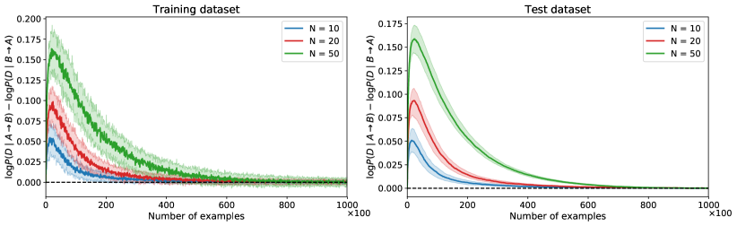
We present experiments comparing the learning curve of the correct causal model on the transfer distribution vs the learning curve of the incorrect model. The adaptation with only a few gradient steps on data coming from a different, but related, transfer distribution is critical in getting a signal that can be leveraged by our meta-learning algorithm. To show the effect of this adaptation, and motivate our use of only a small amount of data from the transfer distribution, we experimented with a model on discrete random variables taking possible values.
In this experiment, we fixed the underlying causal model to be , and trained the modules for each marginal and conditional distributions with maximum likelihood on a large amount of data from some training distribution, as explained in Appendix A. See also Appendix G.1 and Table G.1 for details on the definitions of these modules.
We then adapt all the modules on data coming from a transfer distribution, corresponding on an intervention on the random variable (i.e., the marginal of the ground truth model is modified, while leaving fixed). We used RMSprop for the adaptation, with the same learning rate. For assessing reproducibility and statistical robustness, the experiment was repeated over 100 different training distributions, and over 100 transfer distributions for each training distributions, leading to 10 000 experiments overall. The procedure to acquire different training/transfer distributions is detailed in Appendix G.1.
In Figure 1, we report the log-likelihoods of both models, evaluated on a large test set of 10 000 from the transfer distribution. We can see that as the number of examples from the transfer distribution (equal to the number of adaptation steps) increases, the two models eventually reach the same log-likelihood, reflecting our observation from Appendix A. However the causal model adapts faster than the other model , with the most informative part of the trajectory (where the difference is the largest) is within the first 10 to 20 examples.
2.2.1 Parameter Counting Argument
A simple parameter counting arguments helps us understand what we are observing in Figure 1. First, consider the expected gradient on the parameters of the different modules, during the adaptation phase to the transfer distribution, which we designate as adaptation episode, and corresponds to learning from a meta-example.
Proposition 1
The expected gradient over the transfer distribution of the regret (accumulated negative log-likelihood during the adaptation episode) with respect to the module parameters is zero for the parameters of the modules that (a) were correctly learned in the training phase, and (b) have the correct set of causal parents, corresponding to the ground truth causal graph, if (c) the corresponding ground truth conditional distributions did not change from the training distribution to the transfer distribution.
The proof is given in Appendix B. The basic justification for this proposition is that for the modules that were correctly learned in the training distribution and whose ground truth conditional distribution did not change with the transfer distribution, the parameters already are at a maximum of the log-likelihood over the transfer distribution, so the expected gradient is zero.
As a consequence, the effective number of parameters that need to be adapted, when one has the correct causal graph structure, is reduced to those of the mechanisms that actually changed from the training to the transfer distribution. Since sample complexity - the number of training examples necessary to learn a model - grows approximately linearly (Ehrenfeucht et al., 1989) with VC-dimension (Vapnik and Chervonenkis, 1971), and since VC-dimension grows approximately linearly in the number of parameters in linear models and neural networks Shalev-Shwartz and Ben-David (2014), the learning curve on the transfer distribution will tend to improve faster for the model with the correct causal structure, for which fewer parameters need to be changed. Interestingly, we do not need to have the whole causal graph correctly specified before getting benefits from this phenomenon. If we only have part of the causal graph correctly specified and we change our causal hypothesis to include one more correctly specified mechanism, then we will obtain a gain in terms of the adaptation sample complexity (which shows up when the change in distribution does not touch that mechanism). This nice property also shows up in Proposition 1 (Appendix F), showing a decoupling of the meta-objective across the independent mechanisms.
Let us consider the special case we have been studying up to now. We have four modules, two of which ( and ) are marginal discrete distributions over values, which require each free parameters. The other two modules are conditional probability tables that have rows each with free parameters, i.e., a total of free parameters. If is the correct model and the transfer distribution only changed the true (the cause), and if had been correctly estimated on the training distribution, then for the correct model only parameters need to be re-estimated. On the other hand, because of Bayes’ rule, under the incorrect model (), a change in leads to new parameters for both and , i.e., all parameters must be re-estimated. In this case we see that sample complexity may be for the incorrect model while it would be for the correct model (assuming linear relationship between sample complexity and number of free parameters). Of course, if the change in distribution had been over instead of , the advantage would not have been as great. This would motivate information gathering actions generally resulting in a very sparse change in the mechanisms.
2.3 Smooth parameterization of the causal structure
In the more general case with many more than two hypotheses for the structure of the causal graph, there will be an exponentially large set of possible causal structures explaining the data and we won’t be able to enumerate all of them (and pick the best one after observing episodes of adaptation). However, we can parameterize our belief about an exponentially large set of hypotheses by keeping track of the probability for each directed edge of the graph to be present, i.e., specify for each variable whether some variable is a direct causal parent of (for all pairs in the graph). We will develop such a smooth parametrization further in Appendix F, but it hinges on gradually changing our belief in the individual binary decisions associated with each edge of the causal graph, so we can jointly do gradient descent on all these beliefs at the same time.
In this section, we study the simplest possible version of this idea, representing that edge belief via a structural parameter with , our believed probability that is the correct choice. For that single pair of variables scenario, let us consider two explanations for the data (as in the above sections, for models and ), one with probability and the other with probability . We can write down our transfer objective as a log-likelihood over the mixture of these two models. Note this is different from the usual mixture models, which assume separately for each example that it was sampled from one component or another with some probability. Here, we assume that all of the observed data was sampled from one component or the other. The transfer data regret (negative log-likelihood accumulated along the online adaptation trajectory) under that mixture is therefore as follows:
| (2) |
where and are the online likelihoods of both models respectively on the transfer data. They are defined as
where is the set of transfer examples for a given episode and aggregates all the modules’ parameters as of time step (since the parameters could be updated after each observation of an example from the transfer distribution). is the likelihood of example under some model that has parameters .
The quantity of interest here is , which is our training signal for updating . In the experiments below, after each episode involving transfer examples we update by doing one step of gradient descent, to reduce the transfer negative log-likelihood or regret . What we are proposing is a meta-learning framework in which the inner training loop updates the module parameters (separately) as examples are seen (from either distribution being currently observed), while the outer loop updates the structural parameters (here it is only the scalar ) with respect to the transfer negative log-likelihood.
The gradient of the transfer log-likelihood with respect to the structural parameter is pushing towards the posterior probability that the correct model is and towards the posterior probability that the correct model is :
Proposition 2
The gradient of the negative log-likelihood of the transfer data in Equation (2) wrt. the structural parameter is given by
| (3) |
where is the transfer data, and is the posterior probability of the hypothesis (when the alternative is ). Furthermore, this can be equivalently written as
| (4) |
where is the difference between the log-likelihoods of the two hypotheses on the transfer data .
The proof is given in Appendix D. Note how this posterior probability is basically measuring which hypothesis is better explaining the episode transfer data overall along the adaptation trajectory. is a meta-example for updating the structural parameters like . Larger of one hypothesis over the other leads to moving meta-parameters faster towards the favoured hypothesis. This difference in online accumulated log-likelihoods also relates to log-likelihood scores in score-based methods for structure learning of graphical models (Koller and Friedman, 2009)111One can see as a score attributed to graph , analogously for . The gradient is then pushing toward the graph with the highest score..
To find where SGD converges, note that the actual posterior depends on the prior and thus keeps changing after each gradient step. We are really doing SGD on the expected value of over transfer sets . Equating the gradient of this expected value to zero to look for the stationary convergence point, we thus see on both sides of the equation, and we obtain convergence when the new value of is consistent with the old value, as clarified in this proposition.
Proposition 3
Stochastic gradient descent (with appropriately decreasing learning rate) on with steps from converges towards if , or otherwise.
The proof is given in Section E of the Appendix, and shows that optimizing will end up picking the correct hypothesis, i.e., the one that has the smallest regret (or fastest convergence), measured as the accumulated log-likelihood as adaptation proceeds on the transfer distributions sampled from the distribution , which we can think of like a distribution over tasks, in meta-learning. This analogy with meta-learning also appears in our gradient-based adaptation procedure, which is linked to existing methods like the first-order approximation of MAML (Finn et al., 2017), and its related algorithms (Nichol et al., 2018). Algorithm 1 (Appendix C) illustrates the general pseudo-code for the proposed meta-learning framework.
2.3.1 Experimental Results
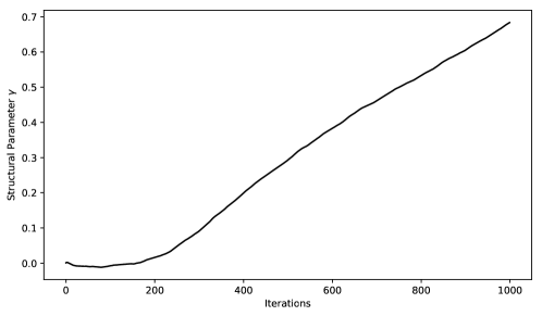
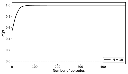
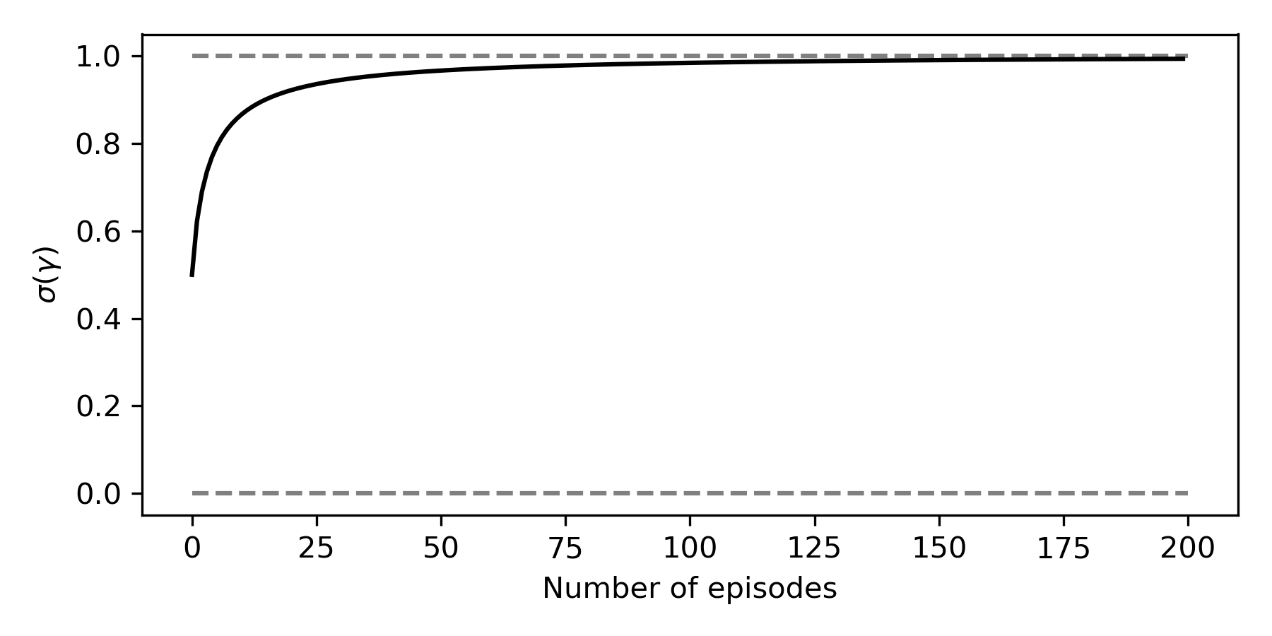
To illustrate the convergence result from Proposition 3, we experiment with learning the structural parameter in a bivariate model, with discrete random variables, each taking and possible values. In this experiment, we assume that the underlying causal model (unknown to the algorithm) is fixed to , so that we want the structural parameter to eventually converge to . The details of the experimental setup can be found in Appendix G.1.
In Figure 2, we show the evolution of (which is the model’s belief of being the correct causal model) as the number of episodes increases. Starting from an equal belief for both and to occur (), the structural parameter converges to within episodes.
This observation is consistent across a range of domains, including models with multimodal or multivariate continuous variables, and different parametrizations of the models. In Appendix G.2, we present results for two discrete variables but using MLPs to parametrize the conditional distributions, and where there are more causal hypotheses: we consider one binary choice for each directed edge in the graph, to decide whether one variable is a direct causal parent or not. Figure 3 shows that the correct causal graph is quickly recovered. To estimate the gradient, we use a generalization of the regret loss (introduced above, Equation (2)) and its gradient, described in Appendix F.
In Appendix G.3, we consider the case of continuous scalar multimodal variables. The ground truth joint distribution is obtained by making the effect a non-linear function of cause , where is a randomly generated spline. Figure G.1 shows an example of a resulting joint distribution. We model the conditionals with mixture density networks (Bishop, 1994) and the marginals by a Gaussian mixture. We obtain results that are similar to the discrete case, with the correct causal interpretation being recovered quickly, as illustrated in Figure G.2.
We also show in Appendix G.4 results on models with two continuous random variables, each being distributed as a multivariate Gaussian, with dimensions. Similar to the experiment with discrete random variables, the same argument about parameter counting mentioned in Section 2.2.1 holds here. Again, we obtain results consistent with the previous examples, where the structural parameter converges to , effectively recovering the correct causal model .
3 Representation Learning
So far, we have assumed that the system has unrestricted access to the true underlying causal variables, and . However in many realistic scenarios for learning agents, the observations available to the learner might not be instances of the true causal variables but sensory-level data instead, like pixels and sounds. If this is the case, our working assumption – that the correct causal graph will be sparsely connected, made of independent components, and affected sparsely by distributional shifts – can not be expected to hold true in general in the space of observed variables. To tackle this, we propose to follow the deep learning objective of disentangling the underlying causal variables (Bengio et al., 2013), and learn a representation in which these properties hold. In the simplest form of this setting, the learner must map its raw observations to a hidden representation space via an encoder . The encoder is trained such that the hidden space helps to optimize the meta-transfer objective described above, i.e., we consider the encoder, along with , as part of the set of structural or meta-parameters to be optimized with respect to the meta-transfer objective.
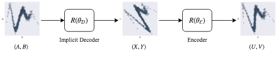
To study this simplified setting, we consider that our raw observations originate from the true causal variables via the action of a ground truth decoder (or generator network) that the learner is not aware of but is implicitly trying to invert, as illustrated in Figure 4. The variables , , and are assumed to be scalars, and we first consider be a rotation matrix such that:
| (5) |
The encoder is set to another rotation matrix, one that maps the observations to the hidden representation as follows:
| (6) |
The causal modules are now to be trained on the variables and in the same way as detailed in Section 2, as if they were observed directly. Indeed, if the encoder is valid one would obtain either or up to a negative sign, but we say in that case and without loss of generality that recovered , corresponding to the solution . In this case, the model is causal and should therefore have an advantage over the anticausal model , as far as adaptation speed on the transfer distribution is concerned. However, if the encoder is not valid, one would obtain superpositions of the form:
| (7) | ||||
| (8) |
where . In the extremum where , it is clear that the model will not have an advantage over the model in terms of regret on the transfer distribution. However, the question we are interested in is whether it is possible to learn the encoder . We verify this experimentally using Algorithm 1, but where the meta-parameters are now both (choosing between cause and effect which is which) and the parameters of the encoder (here the angle of a rotation matrix). The details of that experiment are provided in Appendix H, which illustrates – see Figure 5 – how the proposed objective can disentangle (here in a very simple setting) the ground truth variables (up to permutation).

4 Related Work
Although this paper focuses on the causal graph, the proposed objective is motivated by the more general question of discovering the underlying causal variables (and their dependencies) that explain the environment of a learner and make it possible for that learner to plan appropriately. The discovery of underlying explanatory variables has come under different names, in particular the notion of disentangling underlying variables (Bengio et al., 2013). As stated already by Bengio et al. (2013) and clearly demonstrated by Locatello et al. (2018), assumptions, priors or biases are necessary to identify the underlying explanatory variables. The latter paper (Locatello et al., 2018) also reviews and evaluates recent work on disentangling, and discusses different metrics that have been proposed. An extreme view of disentangling is that the explanatory variables should be marginally independent, and many deep generative models (Goodfellow et al., 2016) and independent component analysis models (Hyvärinen et al., 2001, 2018) are built on this assumption. However, the kinds of high-level variables that we manipulate with natural language are not marginally independent: they are related to each other through statements that are usually expressed in sentences (e.g., a classical symbolic AI fact or rule), involving only a few concepts at a time. This kind of assumption has been proposed to help discover such linguistically relevant high-level representations from raw observations, such as the consciousness prior (Bengio, 2017), with the idea that humans focus at any particular time on just a few concepts that are present to our consciousness. The work presented here could provide an interesting meta-learning objective to help learn such encoders as well as figure out how the resulting variables are related to each other. In that case, one should distinguish two important assumptions: the first one is that the causal graph is sparse (has few edges, as in the consciousness prior (Bengio, 2017) and in some methods to learn Bayes net structure, e.g. (Schmidt et al., 2007)); and the second one is that it changes sparsely due to interventions (which is the focus of this work).
Approaches for Bayesian network structure learning based on discrete search over model structures and simulated annealing are reviewed in Heckerman et al. (1995). There, it has been common to use Minimum Description Length (MDL) principles to score and search over models Lam and Bacchus (1993); Friedman and Goldszmidt (1998), or the Bayesian Information Criterion (BIC) to search for models with high relative posterior probability Heckerman et al. (1995). Prior work such as Heckerman et al. (1995) has also relied upon purely observational data, without the possibility of interventions and therefore focused on learning likelihood or hypothesis equivalence classes for network structures. Since then, numerous methods have also been devised to infer the causal direction from purely observational data (Peters et al., 2017), based on specific, generally parametric assumptions, on the underlying causal graph. Pearl’s seminal work on do-calculus Pearl (1995, 2009); Bareinboim and Pearl (2016) lays a foundation for expressing the impact of interventions on probabilistic graphical models – we use it in our work. In contrast, here we are proposing a meta-learning objective function for learning causal structure, not requiring any specific constraints on causal graph structure, only on the sparsity of the changes in distribution in the correct causal graph parametrization.
Our work is also related to other recent advances in causation, domain adaptation and transfer learning. Magliacane et al. (2018) have sought to identify a subset of features that lead to the best predictions for a variable of interest in a source domain such that the conditional distribution of the variable of interest given these features is the same in the target domain. Johansson et al. (2016) examine counterfactual inference and formulate it as a domain adaptation problem. Shalit et al. (2017) propose a technique called counterfactual regression for estimating individual treatment effects from observational data. Rojas-Carulla et al. (2018) propose a method to find an optimal subset that makes the target independent from the selection variables. To do so, they make the assumption that if the conditional distribution of the target given some subset is invariant across different source domains, then this conditional distribution must also be the same in the target domain. Parascandolo et al. (2017) propose an algorithm to recover a set of independent causal mechanisms by establishing competition between mechanisms, hence driving specialization. Alet et al. (2018) proposed a meta learing algorithm to recover a set of specialized modules, but did not establish any connections to causal mechanisms. More recently, Dasgupta et al. (2019) adopted a meta-learning approach to draw causal inferences from purely observational data.
5 Conclusion and Future Work
We have established in very simple bivariate settings that the rate at which a learner adapts to sparse changes in the distribution of observed data can be exploited to select or optimize causal structure and disentangle the causal variables. This relies on the assumption that with the correct causal structure, those distributional changes are localized and sparse. We have demonstrated these ideas through theoretical results as well as experimental validation. See https://github.com/authors-1901-10912/A-Meta-Transfer-Objective-For-Learning-To-Disentangle-Causal-Mechanisms for source code of the experiments.
This work is only a first step in the direction of optimizing causal structure based on the speed of adaptation to modified distributions. On the experimental side, many settings other than those studied here should be considered, with different kinds of parametrizations, richer and larger causal graphs, different kinds of optimization procedures, etc. Also, much more needs to be done in exploring how the proposed ideas can be used to learn good representations in which the causal variables are disentangled, since we have only experimented at this point with the simplest possible encoder with a single degree of freedom. Scaling up these ideas would permit their application towards improving the way in which learning agents deal with non-stationarities, and thus improving sample complexity and robustness of learning agents.
Acknowledgements
We would like to acknowledge support for this project from NSERC, CIFAR and Canada Research Chairs, as well as the feedback from Rémi Le Priol, Isabelle Lacroix, Alexandre Piché, and Akram Erraqabi. AG would like to thank Sergey Levine, Chelsea Finn, Michael Chang, Abhishek Gupta for useful discussions.
References
- Alet et al. (2018) Ferran Alet, Tomás Lozano-Pérez, and Leslie P Kaelbling. Modular meta-learning. arXiv preprint arXiv:1806.10166, 2018.
- Bareinboim and Pearl (2016) Elias Bareinboim and Judea Pearl. Causal inference and the data-fusion problem. Proceedings of the National Academy of Sciences, 113(27):7345–7352, 2016.
- Bengio (2017) Yoshua Bengio. The consciousness prior. arXiv preprint arXiv:1709.08568, 2017.
- Bengio et al. (2013) Yoshua Bengio, Aaron Courville, and Pascal Vincent. Representation learning: A review and new perspectives. IEEE Trans. Pattern Analysis and Machine Intelligence (PAMI), 35(8):1798–1828, 2013.
- Bishop (1994) Christopher M Bishop. Mixture density networks. Technical report, Citeseer, 1994.
- Dasgupta et al. (2019) Ishita Dasgupta, Jane Wang, Silvia Chiappa, Jovana Mitrovic, Pedro Ortega, David Raposo, Edward Hughes, Peter Battaglia, Matthew Botvinick, and Zeb Kurth-Nelson. Causal Reasoning from Meta-reinforcement Learning. arXiv preprint arXiv:1901.08162, 2019.
- Ehrenfeucht et al. (1989) Andrzej Ehrenfeucht, David Haussler, Michael Kearns, and Leslie Valiant. A general lower bound on the number of examples needed for learning. Information and Computation, 82(3), 1989.
- Finn et al. (2017) Chelsea Finn, Pieter Abbeel, and Sergey Levine. Model-Agnostic Meta-Learning for Fast Adaptation of Deep Networks. International Conference on Machine Learning (ICML), 2017.
- Friedman and Goldszmidt (1998) Nir Friedman and Moises Goldszmidt. Learning bayesian networks with local structure. In Learning in graphical models, pages 421–459. Springer, 1998.
- Goodfellow et al. (2016) Ian J. Goodfellow, Yoshua Bengio, and Aaron Courville. Deep Learning. MIT Press, 2016. URL http://deeplearningbook.org.
- Heckerman et al. (1995) David Heckerman, Dan Geiger, and David M Chickering. Learning bayesian networks: The combination of knowledge and statistical data. Machine learning, 20(3):197–243, 1995.
- Hyvärinen et al. (2001) Aapo Hyvärinen, Juha Karhunen, and Erkki Oja. Independent Component Analysis. Wiley-Interscience, May 2001. ISBN 047140540X.
- Hyvärinen et al. (2018) Aapo Hyvärinen, Hiroaki Sasaki, and Richard E. Turner. Nonlinear ica using auxiliary variables and generalized contrastive learning. CoRR, arXiv:1805.08651, 2018.
- Johansson et al. (2016) Fredrik Johansson, Uri Shalit, and David Sontag. Learning representations for counterfactual inference. In International Conference on Machine Learning, pages 3020–3029, 2016.
- Koller and Friedman (2009) Daphne Koller and Nir Friedman. Probabilistic Graphical Models: Principles and Techniques. MIT press, 2009.
- Lam and Bacchus (1993) Wai Lam and Fahiem Bacchus. Using causal information and local measures to learn bayesian networks. In Proceedings of the Ninth international conference on Uncertainty in artificial intelligence, pages 243–250. Morgan Kaufmann Publishers Inc., 1993.
- Locatello et al. (2018) Francesco Locatello, Stefan Bauer, Mario Lucic, Sylvain Gelly, Bernhard Schölkopf, and Olivier Bachem. Challenging common assumptions in the unsupervised learning of disentangled representations. CoRR, arXiv:1811.12359, 2018.
- Magliacane et al. (2018) Sara Magliacane, Thijs van Ommen, Tom Claassen, Stephan Bongers, Philip Versteeg, and Joris M Mooij. Domain adaptation by using causal inference to predict invariant conditional distributions. In Advances in Neural Information Processing Systems, pages 10869–10879, 2018.
- Nichol et al. (2018) Alex Nichol, Joshua Achiam, and John Schulman. On First-Order Meta-Learning Algorithms. arXiv:1803.02999, 2018.
- Parascandolo et al. (2017) Giambattista Parascandolo, Niki Kilbertus, Mateo Rojas-Carulla, and Bernhard Schölkopf. Learning independent causal mechanisms. arXiv preprint arXiv:1712.00961, 2017.
- Pearl (1995) Judea Pearl. Causal diagrams for empirical research. Biometrika, 82(4):669–688, 1995.
- Pearl (2009) Judea Pearl. Causality. Cambridge university press, 2009.
- Peters et al. (2017) Jonas Peters, Dominik Janzing, and Bernhard Schölkopf. Elements of causal inference: foundations and learning algorithms. MIT press, 2017.
- Rojas-Carulla et al. (2018) Mateo Rojas-Carulla, Bernhard Schölkopf, Richard Turner, and Jonas Peters. Invariant models for causal transfer learning. The Journal of Machine Learning Research, 19(1):1309–1342, 2018.
- Schmidt et al. (2007) Mark W. Schmidt, Alexandru Niculescu-Mizil, and Kevin P. Murphy. Learning graphical model structure using l1-regularization paths. In AAAI, 2007.
- Shalev-Shwartz and Ben-David (2014) Shai Shalev-Shwartz and Shai Ben-David. Understanding Machine Learning - from Theory to Algorithms. Cambridge University Press, 2014.
- Shalit et al. (2017) Uri Shalit, Fredrik D Johansson, and David Sontag. Estimating individual treatment effect: generalization bounds and algorithms. In Proceedings of the 34th International Conference on Machine Learning-Volume 70, pages 3076–3085. JMLR. org, 2017.
- Vapnik and Chervonenkis (1971) V. N. Vapnik and A. Y. Chervonenkis. On the uniform convergence of relative frequencies of events to their probabilities. Theory of Probability and its Applications, 16:264–280, 1971.
A Results on Non-Identifiability of Causal Structure
We show here that the maximum likelihood estimation of both models specified in Equation (2.1) yields the same estimated distribution over and , i.e., the joint likelihood on the training distribution is not sufficient to distinguish the and causal models, in the non-parametric case (no assumption at all on the family of distributions). Let
We now state the maximum likelihood estimators for each models:
| (9) |
where is the total number of observations, the number of times we observed , the number of times we observed and the number of times we observed and jointly. We can now compute the likelihood for each model:
| (10) |
which is what we intended to show. To illustrate this result, we also experiment with learning the modules for both models and with SGD. In Figure A.1, we show the difference in log-likelihoods between these two models, evaluated on training and test data sampled from the same distribution, during training. We can see that while the model fits the data faster than the other model (corresponding to a positive difference in Figure A.1), both models achieve the same log-likelihoods on both models at convergence. This shows that the two models are indistinguishable based on data sampled from the same distribution, even on test data.
B Proof of the Zero-Gradient Proposition
Let us restate more formally and prove Proposition 1.
Proposition 0
Consider conditional probability modules where indicates that is among the parents of in a directed acyclic causal graph. Consider ground truth training distribution and transfer distribution over these variables, and ground truth causal structure . The joint log-likelihood for a sample with respect to the module parameters decomposed into module parameters is . If (a) a model has the correct causal structure , and (b) it been trained perfectly on , leading to estimated parameters , and (c) the ground truth and only differ from each other only for some for , then for .
Proof Let be the subset of excluding . We can simplify the expected gradient as follows.
where the second equality is obtained because does not influence module , and is the same for conditionals with (assumption (c)). Now for the special case of , we obtain
| (12) |
where the second equality arises from assumption (b), and the last line from zeroing the inner sum via the general identity
C Pseudo-Code
D Proof of the Structural Parameter Gradient Proposition
Let us restate more formally and prove Proposition 2.
Proposition 0
The gradient of the negative log-likelihood regret of the transfer data
with respect to the structural parameter (where ) is given by
| (13) |
where is the transfer data, and is the posterior probability of the hypothesis (when the alternative is ), defined by applying Bayes rule to . Furthermore, this can be equivalently written as
| (14) |
where is the difference between the log-likelihoods of the two hypotheses on transfer data .
Proof First note that, using Bayes rule,
| (15) |
where is the online likelihood of the transfer data under the mixture, so that the regret is . For the second line above, note that
| (16) |
where encapsulates the information about (through some adaptation procedure). Since we only consider the two hypotheses and , we also have . Then
| (17) |
which concludes the first part of the proof. Moreover, in order to prove the equivalent formulation in Equation (14), it is sufficient to prove that . Using the logit function , and the expression in Equation (15), we have
| (18) |
E Proof of the Proposition on the Convergence Point of Gradient Descent on the Structural Parameter
We use the same notation as in the above proof and statement.
Proposition 0
Stochastic gradient descent (with appropriately decreasing learning rate) on , with and with steps following converges towards if , or otherwise.
Proof We are going to consider the fixed point of gradient descent when the gradient is zero, since we already know that SGD converges with an appropriately decreasing learning rate. Let us introduce some notation to simplify the algebra: , , so , and define , and . Framing the stationary point in terms of rather than gives us the inequality constraints and and no equality constraint. Applying the KKT conditions with constraint functions and gives us
| (19) |
We already see from the last two equations that if (i.e. excluding 0 and 1), we must have , i.e., (with drop the subscript on when it is clear from context). Let us study that case first and show that it leads to an inconsistent set of equations (thus forcing the solution to be either or ). Let us rewrite the gradient to highlight in it:
| (20) |
The KKT conditions with the above two inequality constraints for give
| (21) |
If we consider the solutions (i.e., ) we now show that we get a contradiction. First note that to satisfy the above equation with means that either or (which is inconsistent with the assumption that ) or that . Let us consider that equation, and since and we can either multiply by or by on both sides. Assuming and multiplying by gives
| (22) |
For this equation to be satisfied, we need all the time, since by construction. This would however correspond to . Similarly, assuming we can multiply the stationarity equation by and get
| (23) |
Again, this can only be 0 if all the time, i.e., . We conclude that the solutions are not possible because they would lead to inconsistent conclusions, which leaves only or . When we have , and when we have . Thus the minimum will be achieved at when , or otherwise.
F More Than Two Causal Hypotheses
In this section, we consider one approach to generalize to more than two causal structures. We consider variables, corresponding to possible causal graphs, since each variable could be (or not) a direct cause of any variable , leading to binary decisions. Note that a causal graph can in principle have cycles (if time is not measured with sufficient precision), although having a directed acyclic graph allows a much simpler sampling procedure (ancestral sampling). In our experiments the ground truth graph will always be directed, to make sampling easier and faster, but the learning procedure will not directly assume that. Motivated by the mechanism independence assumption, we propose a heuristic to learn the causal graph in which we independently parametrize the binary probability that is a parent (direct cause) of . As was the case for Section 2, we parametrize this Binomial distribution via binary edges that specify the graph structure:
| (24) |
where . Let us define the parents of , given , as the set of ’s such that :
| (25) |
where is the bit vector with elements (and is ignored). Similarly, we could parametrize the causal graph with a structural causal model where some of the inputs (from variable ) of each function (for variable ) can be ignored with some probability :
| (26) |
where is an independent noise source to generate and parametrizes the generator (as in a GAN), while not being allowed to use variable unless (and of course not being allowed to use ). We can consider that is a kind of neural network similar to the denoising auto-encoders or with dropout on the input, where is a binary mask vector that prevents from using some of the ’s (for which ).
The conditional likelihood measures how well the model that uses the incoming edges for node performs for example . We build a multiplicative (or exponentiated) form of regret by multiplying these likelihoods as changes during an adaptation episode, for node :
| (27) |
The overall exponentiated regret for the given graph structure is . Similarly to the bivariate case, we want to consider a mixture over all the possible graph structures, but where each component must explain the whole adaptation sequence, thus we define as a loss for the generalized multi-variable case
| (28) |
Note the expectation over the possible values of , which is intractable. However, we can still get an efficient stochastic gradient estimator, which can be computed separately for each node of the graph (with samples arising only out of , the incoming edges into ):
Proposition 1
The overall regret (Equation (28)) rewrites
| (29) |
and if we are willing to consider multiple samples of in parallel, a biased but asymptotically unbiased (as the number of these samples increases to infinity) estimator of the gradient of the overall regret with respect to meta-parameters can be defined:
| (30) |
where the (k) index indicates the values obtained for the -th draw of .
Proof Recall that so we can rewrite the regress loss as follows:
| (31) |
So the regret gradient on meta-parameters of node is
| (32) |
Note that with the sigmoidal parametrization of ,
as in the cross-entropy loss. Its gradient can similarly be simplified to
| (33) |
A biased but asymptotically unbiased estimator of is thus obtained by sampling graphs (over which the means below are run):
| (34) |
where index (k) indicates the -th draw of , and we obtain a weighted sum of the individual binomial gradients weighted by the relative regret of each draw of ,
leading to Equation (30).
This decomposition is good news because the loss is a sum of independent
terms, one per node , depending only of and and similarly only
depends on rather than the
full graph structure. We use the
estimator from Equation (30) in the general pseudo-code for meta-transfer learning of causal structure displayed in Algorithm 1.
G Results on Learning which is Cause and which is Effect
In order to assess the performance of our meta-learning algorithm, we applied it on generated data from three different domains: discrete random variables, multimodal continuous random variables and multivariate gaussian-distributed variables. In this section, we describe the setups for all three experiments, along with additional results to complement the results described in the main text. Note that in all these experiments, we fix the structure of the ground-truth to be , and only perform interventions on the cause .
G.1 Discrete variables and Two Causal Hypotheses
We consider a bivariate model, where both random variables are sampled from a categorical distribution. The underlying ground-truth model can be described as
| (35) |
with is a probability vector of size , and is a probability vector of size , which depends on the value of the variable . In our experiment, each random variable can take one of values. Since we are working with only two variables, the only two possible models are:
-
•
Model :
-
•
Model :
We build 4 different modules, corresponding to the model of each possible marginal and conditional distribution. These modules’ definition and their corresponding parameters are shown in Table G.1.
| Distribution | Module | Parameters | Dimension | |
|---|---|---|---|---|
| Model | ||||
| Model | ||||
In order to get a set of initial parameters, we first train all 4 modules on a training distribution. This training distribution corresponds to a fixed choice of and (for all possible values of ). Note that the superscript in emphasizes the fact that this defines the distribution prior to intervention, with the mechanism being unchanged by the intervention. These probability vectors are sampled randomly from a uniform Dirichlet distribution
| (36) |
Given this initial training distribution, we can sample a large dataset of training examples from the ground-truth model, using ancestral sampling.
| (37) |
Using this large dataset from the training distribution, we can train all 4 modules using gradient descent, or any other advanced first-order optimizer, like RMSprop. The parameters , , & of the different modules found after this initial training will be used as the initial parameters for the adaptation on a new transfer distribution.
Similar to the way we defined the training distribution, we can define a transfer distribution as a soft intervention on the random variable . In this experiment, this accounts for changing the distribution of , that is with a new probability vector , also sampled randomly from a uniform Dirichlet distribution
| (38) |
To perform adaptation on the transfer distribution, we also sample a smaller dataset of transfer examples , with the size of the training set. In our experiment, we used transfer examples. We also used ancestral sampling on this new transfer distribution to acquire samples, similar to Equation (37) (with instead of ).
Starting from the parameters estimated after the initial training on the training distribution, we perform a few steps of adaptation on the modules parameters , , & using steps of gradient descent based on the transfer dataset . The value of the likelihoods for both models is recorded as well, and computed as
| (39) |
where represents a mini-batch of examples from , and the superscript on the parameters highlights the fact that these likelihoods are computed after steps of adaptation. This product over ensures that we monitor the progress of adaptation along the whole trajectory. In this experiment, we used steps of gradient descent on mini-batch of size 10 for the adaptation.
Finally, in order to update the structural parameter , we can use Proposition 2 to compute the gradient of the loss with respect to :
| (40) | ||||
| (41) |
where . The update of can be one step of gradient descent, or using any first-order optimizer like RMSprop. We perform multiple interventions over the course of meta-training by sampling multiple transfer distributions, and following the same steps of adaptation and update of the structural parameter .
In Figure 2, we report the evolution of the structural parameter (or rather, ) as a function of the number of meta-training steps or, similarly, the number of different interventions made on the causal model. The model’s belief indeed converges to , proving that the algorithm was capable of recovering the correct causal direction .
G.2 Discrete Variables with MLP Parametrization
We consider a bivariate model similar to the ones defined above, where each random variable is sampled from a categorical distribution. Instead of expressing probabilities in a tabular form, we train simple feed-foward neural networks (MLP), one per conditional variable. MLP is the independent mechanism of causal variable that determines the conditional probability of the discrete choices for variable , given its parents.
Each MLP receives concatenated -dimensional one-hot vectors, masked appropriately according to the chosen causal structure , i.e., with the -th input of the -th MLP being multiplied by . Each directed edge presence or absence is thus indicated by , with if variable is a direct causal parent of variable . The MLP maps the input units through one hidden layer that contains hidden units and a ReLU non-linearity, and then maps the hidden units to output units and a softmax representing a predicted categorical distribution.
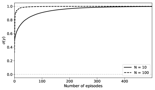
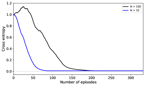
The causal structure belief is specified by an matrix , with the estimated probability that variable is directly caused by variable . The causal structure is drawn from , as per Algorithm 1. We generalize the estimator introduced for the 2-hypotheses case as per Appendix F, i.e., we use the gradient estimator in Equation 30.
To evaluate the correctness of the structure being learnt, we measure the cross entropy between the ground-truth SCM and the learned SCM. In Figure 3 we show this cross-entropy over different episodes of training for bivariate discrete distributions with either 10 categories or 100 categories. Both models are first pretrained for 100 examples with fully connected edges before starting training on the transfer distributions.
G.3 Continuous Multimodal Variables
Consider a family of joint distributions over the causal variables and sampled from the structural causal model (SCM):
| (42) |
where is a randomly generated spline and is sampled i.i.d from the unit-normal distribution.
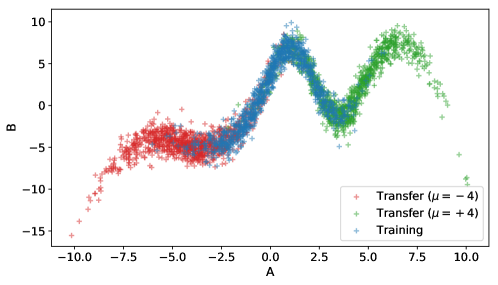
To obtain the spline, we sample the points uniformly spaced from the interval , and another points uniform randomly from the interval . This yields pairs , which make the knots of a second-order spline. We set , for our experiments. In Figure G.1, we plot samples from one such SCM for the training distribution () and two transfer distributions ().
The conditionals and are parameterized as 2-layer Mixture Density Networks Bishop (1994) with hidden units and components. The marginals and are parameterized as Gaussian Mixture Models, also with components. The training now follows as described below.
Similar to Appendix G.1, we first pre-train the modules corresponding to the conditionals and marginals on the training distribution. To that end, we select as the training distribution, sample a (large) training dataset from it using ancestral sampling, and solve the following two problems independently until convergence:
| (43) | ||||
| (44) |
The adaptation performance of and models can now be evaluated on transfer distributions. For a sampled uniformly in , we select as the transfer distribution, and denote with samples from it. Both models are fine-tuned on for iterations (see Algorithm 1), and the area under the corresponding negative-log-likelihood curves becomes the regret:
| (45) |
and likewise for . In these experiments, the modules corresponding to the marginals (ie. GMM) are learned offline via Expectation Maximization, and we denote with the trained model. These can now be used to define the following meta-objective for the structural meta-parameter :
| (46) |
The structural regret is now minimized with respect to for 200 iterations (updates of ). Figure G.2 shows the evolution of as training progresses. This is expected, given that we expect the causal model to perform better on the transfer distributions, i.e. we expect in expection. Consequently, assigning a larger weight to optimizes the objective.
G.4 Linear Gaussian Model
In this experiment, the two variables we consider are vectors (i.e. and ). The ground truth causal model is given by
| (47) |
where , and . and are covariance matrices222Ground truth parameters , and are sampled from a Gaussian distribution, while and are sampled from an inverse Wishart distribution.. In our experiments, . Once again, we want to identify the correct causal direction between and . To do so, we consider two models: and . We parameterize both models symmetrically:
| (48) |
Note that each covariance matrix is parameterized using the Cholesky decomposition. Unlike previous experiments, we are not conducting any pre-training on actual data. Instead, we fix the parameters of both models to their exact values according to the ground truth parameters introduced in Equation G.4. For model , this can be done trivially. For the second model, we can compute its exact parameters analytically. Once the exact parameters are set, both models are equivalent in the sense that .
Each meta-learning episode starts by initializing the parameters of both models to the values identified during the pre-training. Afterward, a transfer distribution is sampled (i.e. ). Then, both models are trained on samples from this distribution, for 10 iterations only. During this adaptation, the log-likelihoods of both models are accumulated in order to compute and . At this stage, we compute the meta objective estimate , compute its gradient w.r.t. and update .
Figure G.3 shows that, after 200 episodes, converges to 1, indicating the success of the method on this particular task.
H Results on Learning the Correct Encoder
The causal variables are sampled from the distribution described in Eqn G.3, and are mapped to observations via a hidden (and a priori unknown) decoder , where is a rotation matrix. The observations are then mapped to the hidden state via the encoder . The computational graph is depicted in Figure 4.
Analogous to Equation 46 in Appendix G.3, we now define the regret over the variables instead of :
| (49) |
where the dependence on is implicit in . In every meta-training iteration, the and models are trained on the training distribution for iterations. Subsequently, the regrets and are obtained by a process identical to that described in Equation 45 of Appendix G.3 (albeit with variables and ). Finally, the gradients of are evaluated and the meta-parameters and are updated. This process is repeated for meta-iterations, and Figure 5 shows the evolution of as training progresses (where has been set to ). Further, Figure H.1 shows the corresponding evolution of the structural parameter .