Zero Rest Mass Soliton Solutions

Abstract

In this paper, extended Klein-Gordon field systems will be introduced. Theoretically, it will be shown that for a special example of these systems, it is possible to have a single zero rest mass soliton solution, which is forced to move at the speed of light provided it is considered a non-deformed rigid object. This special soliton solution has the minimum energy among the other solutions, i.e. any arbitrary deformation in its internal structure leads to an increase in the total energy.

Keywords : zero rest mass; soliton; stability; extended Klein-Gordon; solitary wave

I Introduction

The classical relativistic field theory with soliton solutions is an attempt to model particles as some stable localized non-singular objects. Solitons are the stable solitary wave solutions of the nonlinear field systems whose energy density functions are localized and satisfies the standard relativistic energy-rest mass-momentum relations properly rajarama ; Das ; lamb ; Drazin . A well-known example for solitons in $1+1$ dimensions are kink and anti-kink solutions of the real nonlinear Klein-Gordon (KG) systems phi41 ; phi42 ; phi43 ; phi44 ; phi45 ; OV ; GH ; MM1 ; MR ; phi62 ; DSG1 ; DSG2 ; DSG3 ; MM2 ; waz ; Kink1 ; Kink2 ; Kink3 ; Kink4 ; Kink5 ; Kink6 ; Kink7 . For the complex nonlinear KG systems, it was shown that there are some localized soliton (-like) solutions that are called Q-balls Vak3 ; Vak4 ; Vak5 ; Vak6 ; Lee3 ; Scoleman ; R1 ; R2 ; R3 ; R4 ; R5 ; R6 ; R7 ; R8 ; Riazi2 ; MM3 . Morover, the Skyrme model SKrme ; SKrme2 and ’t Hooft Polyakov model toft ; pol are also two well-known relativistic field models, which yield soliton solutions in $3+1$ dimensions.

All well-known relativistic linear and nonlinear scalar field systems, which have been used in the classical or quantum field theory, are in the standard mathematical formats that can be called (nonlinear) KG (-like) systems. In this work, the extended KG systems for scalar fields are introduced as well. Theoretically, we show that for a special extended KG system in $1+1$ dimensions, as a simple example, it is possible to have a soliton solution with zero rest mass (or zero energy). The other non-trivial solutions of this special system all have non-zero positive rest energies. In fact, the massless soliton solution is a special single solution among the others with the least amount of energy. This massless solution, if it is considered a non-deformed rigid object, responds to any amount of force, no matter how tiny, by immediately accelerating to the speed of light. This model can be simply extended to $3+1$ dimensions to have a particle-like solution with zero rest mass. In general, if one considers such a massless particle in the space, since there is no area in the space with absolute zero interaction, it has to move at the speed of light, exactly according to the special relativity.

The organization of this paper is as follows. In section 2, the (nonlinear) KG systems and the extended KG systems are introduced. In section 3, a special extended KG system is introduced, which leads to a stable massless soliton solution. The last section is devoted to the summary and conclusions.

II The (nonlinear) KG systems and the extended KG systems

In the standard relativistic field theory, different systems can be identified with different Lagrangian densities. The standard Lagrangian densities are considered to be functions of several fields $\phi_{r}$ ($r=1,\ldots,N$) and their first derivatives ($\phi_{r,\alpha}=\frac{\partial\phi_{r}}{\partial x^{\alpha}}$):

$${\cal L}={\cal L}(\phi_{r},\phi_{r,\alpha}).$$ (1)

According to the principle of least action, the related equations of motion would be,

$$\frac{\partial{\cal L}}{\partial\phi_{r}}-\frac{\partial}{\partial x^{\mu}}\left(\frac{\partial{\cal L}}{\partial\phi_{r,\mu}}\right)=0.$$ (2)

In general, since the Lagrangian density (1) is invariance under space-time translations $x^{\mu}\rightarrow x^{\mu}+a^{\mu}$, four continuity equations $\partial_{\mu}T^{\mu\nu}=0$ and hence four conserved quantities $P^{\mu}=\int T^{o\mu}d^{3}\textbf{x}$ are obtained where,

$$T^{\mu\nu}=\frac{\partial{\cal L}}{\partial\phi_{r,\mu}}\frac{\partial\phi_{r}}{\partial x_{\nu}}-{\cal L}g^{\mu\nu}$$ (3)

is called the energy-momentum tensor and $g^{\mu\nu}$ the $3+1$ dimensional Minkowski metric. Note that, in this paper, for simplicity, we take the speed of light equal to one ($c=1$). For any arbitrary solution for which the components of the energy-momentum tensor $T^{\mu\nu}$ asymptomatically approach zero at infinity, the four conserved quantities $P^{\mu}=\int T^{o\mu}d^{3}\textbf{x}$ form a four vector, which is called the energy-momentum four vector. So, for all localized solutions of equation (2), the standard relativistic energy-rest mass-momentum relations satisfied generally:

$$E=m=P^{0}\equiv\int T^{00}d^{3}\textbf{x}=\gamma E_{o}=\gamma m_{o},$$ (5)

$$\textbf{P}=(P^{1},P^{2},P^{3})=\int\left(T^{01},T^{02},T^{03}\right)d^{3}\textbf{x}=\gamma m_{o}\textbf{v}.$$

Note that, $E_{o}$ ($m_{o}$) is the rest energy (mass) for a non-moving localized solution and $E$ ($m$) is the total energy (mass) for its moving version.

Many of the known standard Lagrangian densities, which are used in quantum or classical relativistic field theory, are in the same formats that can be called (nonlinear) KG (-like) Lagrangian densities. The (nonlinear) KG Lagrangian densities can be defined as the linear functions of the kinetic scalar terms ${\cal S}_{ij}={\cal S}_{ji}=\partial_{\mu}\phi_{i}\partial^{\mu}\phi_{j}$, i.e.

$${\cal L}=\sum_{j\geqslant i}^{N}\sum_{i}^{N}\alpha_{ij}(\phi_{1},\cdots,\phi_{N}){\cal S}_{ij}-V(\phi_{1},\cdots,\phi_{N}),$$ (6)

where $\phi_{i}$ must be some scalar fields (not a vector field $\phi_{i\mu}$, like electromagnetic vector field $A^{\mu}$), $V$ (field potential) and coefficients $\alpha_{ij}$’s all are functions of the scalar fields. For example, if one considers a complex scalar field $\phi_{1}=\phi$ ($\phi_{2}=\phi^{*}$ ), the allowed kinetic scalar terms are ${\cal S}_{11}=\partial_{\mu}\phi\partial^{\mu}\phi$, ${\cal S}_{22}=\partial_{\mu}\phi^{*}\partial^{\mu}\phi^{*}$ and ${\cal S}_{12}=\partial_{\mu}\phi\partial^{\mu}\phi^{*}$. Note that the permissible combinations of the kinetic scalars must be ones for which the constructed Lagrangian density (6) is a real functional. For example, the known complex nonlinear KG Lagrangian densities, which yield non-topological particle-like solutions (Q-balls) Vak3 ; Vak4 ; Vak5 ; Vak6 ; Lee3 ; Scoleman ; R1 ; R2 ; R3 ; R4 ; R5 ; R6 ; R7 ; R8 ; Riazi2 ; MM3 , are introduced as follows:

$${\cal L}=\partial_{\mu}\phi^{*}\partial^{\mu}\phi-V(|\phi|)={\cal S}_{11}-V(|\phi|),$$ (7)

for which $\alpha_{11}=\alpha_{22}=0$ and $\alpha_{12}=1$. Equivalently, one can decompose complex scalar field $\phi$ into two distinct real and imaginary parts $\phi_{1}=\phi_{r}$ and $\phi_{2}=\phi_{i}$ (i.e. $\phi=\phi_{r}+i\phi_{i}$). In this representation, the allowed kinetic scalar terms are ${\cal S}_{11}=\partial_{\mu}\phi_{r}\partial^{\mu}\phi_{r}$, ${\cal S}_{22}=\partial_{\mu}\phi_{i}\partial^{\mu}\phi_{i}$ and ${\cal S}_{12}=\partial_{\mu}\phi_{r}\partial^{\mu}\phi_{i}$, respectively. Therefore, the Lagrangian density (7) becomes,

$${\cal L}=\partial_{\mu}\phi_{r}\partial^{\mu}\phi_{r}+\partial_{\mu}\phi_{i}\partial^{\mu}\phi_{i}-V(\sqrt{\phi_{r}^{2}+\phi_{i}^{2}}),$$ (8)

for which $\alpha_{11}=\alpha_{22}=1$ and $\alpha_{12}=0$. Moreover, instead of scalars fields $\phi$ and $\phi^{*}$, one can change the variables to the polar fields $R(x^{\mu})$ and $\theta(x^{\mu})$ as defined by,

$$\phi(x,y,z,t)=R(x,y,z,t)\exp[i\theta(x,y,z,t)].$$ (9)

In the representation of polar fields, $\phi_{1}=R=|\phi|=\sqrt{\phi\phi^{*}}$ is the module scalar field and $\phi_{2}=\theta$ is the phase scalar field, while the allowed kinetic scalar terms are ${\cal S}_{11}=\partial_{\mu}R\partial^{\mu}R$, ${\cal S}_{22}=\partial_{\mu}\theta\partial^{\mu}\theta$ and ${\cal S}_{12}=\partial_{\mu}R\partial^{\mu}\theta$. In terms of polar fields, the Lagrangian-density (7) becomes,

$${\cal L}=(\partial^{\mu}R\partial_{\mu}R)+R^{2}(\partial^{\mu}\theta\partial_{\mu}\theta)-V(R)=({\cal S}_{11})+R^{2}({\cal S}_{22})-V(R),$$ (10)

for which $\alpha_{11}=1$, $\alpha_{22}=R^{2}$ and $\alpha_{12}=0$. Therefore, due to different equivalent fields (representations), there are different kinetic scalars and one can use them to introduce any arbitrary new (nonlinear) KG system.

As previously mentioned, the (nonlinear) KG systems are linear functions of the kinetic scalar terms ${\cal S}_{ij}$ (6). It is possible to consider systems, which are not linear in terms of the kinetic scalars ${\cal S}_{ij}$. We can call them ”extended KG systems”, which are essentially nonlinear. Namely, for a complex field in the polar representation, i.e. $\phi_{1}=R$ and $\phi_{2}=\theta$, the following Lagrangian densities are some examples of the extended KG systems:

$${\cal L}=(\partial^{\mu}R\partial_{\mu}R)(\partial^{\mu}\theta\partial_{\mu}\theta)-V(R)=({\cal S}_{11})({\cal S}_{22})-V(R),$$ (11)

$${\cal L}=(\partial^{\mu}R\partial_{\mu}R)+R^{2}(\partial^{\mu}\theta\partial_{\mu}\theta)^{2}-V(R)=({\cal S}_{11})+R^{2}({\cal S}_{22})^{2}-V(R),$$ (12)

$${\cal L}=\left[(\partial^{\mu}R\partial_{\mu}R)+R^{2}(\partial^{\mu}\theta\partial_{\mu}\theta)-V(R)\right]^{2}=\left[({\cal S}_{11})+R^{2}({\cal S}_{22})-V(R)\right]^{2}$$ (13)

$${\cal L}=\left[(\partial^{\mu}R\partial_{\mu}R)+R^{2}(\partial^{\mu}\theta\partial_{\mu}\theta)\right]^{2}-V(R)=\left[({\cal S}_{11})+R^{2}({\cal S}_{22})\right]^{2}-V(R)$$ (14)

For an extended one, it is expected to encounter very complicated equations and other properties. Although it is not usual to use extended KG systems in standard (quantum or classical) field theory, in this paper it will be shown that using some special extended KG Lagrangian densities can lead to some interesting particle-like solutions with zero rest masses.

III An extended KG system with a single massless soliton solution in $1+1$ dimensions

In this section, we are going to show that it is possible to have an extended KG system in $1+1$ dimensions with a single non-trivial massless stable particle-like solution. A similar model can be introduced in $3+1$ dimensions. However for simplicity, we restrict ourself in $1+1$ dimensions. To achieve this goal, we can consider an extended KG system for a single complex scalar field $\phi~{}(=Re^{i\theta})$, or equivalently for two independent scalar fields $\phi_{1}=R$ and $\phi_{2}=\theta$, in the following form:

$${\cal L}=\sum_{i=1}^{3}{\cal K}_{i}^{3},$$ (15)

where

$${\cal K}_{1}=R^{2}[{\cal S}_{22}-2],$$ (16)

$${\cal K}_{2}=R^{2}[{\cal S}_{22}-2]+[{\cal S}_{11}-4R^{4}+4R^{3}],$$ (17)

$${\cal K}_{3}=R^{2}[{\cal S}_{22}-2]+[{\cal S}_{11}-4R^{4}+4R^{3}]+2R[{\cal S}_{12}],$$ (18)

in which, ${\cal S}_{11}=\partial_{\mu}R\partial^{\mu}R$, ${\cal S}_{22}=\partial_{\mu}\theta\partial^{\mu}\theta$, ${\cal S}_{12}=\partial_{\mu}R\partial^{\mu}\theta$. The related equations of motion can be obtained easily:

$$\sum_{i=1}^{3}{\cal K}_{i}\left[2(\partial_{\mu}{\cal K}_{i})\frac{\partial{\cal K}_{i}}{\partial(\partial_{\mu}R)}+{\cal K}_{i}\partial_{\mu}\left(\frac{\partial{\cal K}_{i}}{\partial(\partial_{\mu}R)}\right)-{\cal K}_{i}\frac{\partial{\cal K}_{i}}{\partial R}\right]=0,$$ (19)

$$\sum_{i=1}^{3}{\cal K}_{i}\left[2(\partial_{\mu}{\cal K}_{i})\frac{\partial{\cal K}_{i}}{\partial(\partial_{\mu}\theta)}+{\cal K}_{i}\partial_{\mu}\left(\frac{\partial{\cal K}_{i}}{\partial(\partial_{\mu}\theta)}\right)\right]=0.$$ (20)

The energy density that belongs to the new extended Lagrangian density (15), would be,

$$\varepsilon(x,t)=T^{00}=\sum_{i=1}^{3}{\cal K}_{i}^{2}\left[3C_{i}-{\cal K}_{i}\right]=\varepsilon_{1}+\varepsilon_{2}+\varepsilon_{3},$$ (21)

which is divided into three distinct parts, in which,

$$C_{i}=\dfrac{\partial{\cal K}_{i}}{\partial\dot{\theta}}\dot{\theta}+\dfrac{\partial{\cal K}_{i}}{\partial\dot{R}}\dot{R}=\begin{cases}\quad\quad 2R^{2}\dot{\theta}^{2}&\text{i=1}\\ 2(\dot{R}^{2}+R^{2}\dot{\theta}^{2})&\text{i=2}\\ 2(\dot{R}+R\dot{\theta})^{2}&\text{i=3}.\end{cases}$$ (22)

After a straightforward calculation, we obtain:

$$\varepsilon_{1}={\cal K}_{1}^{2}[5R^{2}\dot{\theta}^{2}+R^{2}\theta^{\prime 2}+2R^{2}],$$ (23)

$$\varepsilon_{2}={\cal K}_{2}^{2}[5R^{2}\dot{\theta}^{2}+5\dot{R}^{2}+R^{2}\theta^{\prime 2}+R^{\prime 2}+U(R)],$$ (24)

$$\varepsilon_{3}={\cal K}_{3}^{2}[5(R\dot{\theta}+\dot{R})^{2}+(R\theta^{\prime}+R^{\prime})^{2}+U(R)],$$ (25)

where the dot and prime denote differentiation with respect to $t$ and $x$ respectively, and

$$U(R)=4R^{4}-4R^{3}+2R^{2},$$ (26)

is an ascending function, which is bounded from below by zero. Therefore, all terms in equations (23), (24) and (25) are positive definite and then the energy density function (21) is bounded from below by zero too. Hence, at any arbitrary space-time point, the possible minimum value of the energy density function (21) is zero. For example, for the trivial solution $R=0$, i.e. the vacuum state, the energy density function would be zero everywhere. Moreover, there is a single non-trivial localized solution for which the energy density function (21) is zero everywhere. In fact, it is a non-trivial localized solitary wave solution with zero energy (rest mass) as well.

In general, according to equations (19), (20), (23), (24) and (25), it is obvious that the special solutions with zero (rest) energies are ones for which ${\cal K}_{i}$ ($i=1,2,3$) all are zero simultaneously. Therefore, to obtain such special solutions, in general, three conditions ${\cal K}_{i}=0$ ($i=1,2,3$) must be satisfied simultaneously, which lead to three independent nonlinear partial differential equations (PDEs) for two independent scalar fields $R$ and $\theta$ as follows:

$$\partial_{\mu}\theta\partial^{\mu}\theta=2,$$ (27)

$$\partial_{\mu}R\partial^{\mu}R=4R^{4}-4R^{3},$$ (28)

$$\partial_{\mu}R\partial^{\mu}\theta=0,$$ (29)

which do not have any common solution except a trivial solution $R=0$ and a single non-trivial solitary wave solution in the following form:

$$R_{s}(x)=\dfrac{1}{1+x^{2}},\quad\quad\theta_{s}(t)=\omega_{s}t,$$ (30)

which is at rest and $\omega_{s}=\pm\sqrt{2}$ can be called ”the rest frequency”. Using the Lorentz transformations, the moving version of this special solution (30) can be obtained easily as follows:

$$R_{v}(x,t)=\dfrac{1}{1+\gamma^{2}(x-vt)^{2}},\quad\quad\theta_{v}(x,t)=k_{\mu}x^{\mu},$$ (31)

in which $v$ is the velocity, $\gamma=1/\sqrt{1-v^{2}}$ and $k^{\mu}\equiv(\omega,k)$ is a $1+1$ vector, provided

$$k={\omega}v,$$ (32)

and

$$\omega=\gamma\omega_{s}.$$ (33)

Since the energy density function (21) is positive definite, therefore the special solution (30), for which ${\cal K}_{i}=0$ ($i=1,2,3$), definitely has the minimum rest energy ($E_{o}=0$) among the other solutions, i.e. it is a soliton solution. More precisely, for any non-trivial solution of the equations (19) and (20), except the special solution (30), three independent conditions (27), (28) and (29), as three independent PDEs, are not possible to satisfied simulatively. Therefore, for other solutions of the dynamical equations (19) and (20), at least one of the independent scalars ${\cal K}_{i}$ takes non-zero value, which leads to a non-zero positive energy density function (see equations (23), (24) and (25)), i.e. the rest energy is zero just for the single solitary wave solution (30), and for other non-trivial unknown solutions lead to non-zero positive values. In other words, for any arbitrary deformation above the background of the special solution (30) (i.e. $R=R_{s}+\delta R$ and $\theta=\theta_{s}+\delta\theta$), the total energy always increases. For example, for eight different arbitrary small deformations which are introduced as follows:

$$R=\dfrac{1}{1+x^{2}}+\xi e^{-x^{2}},\quad\quad\theta=\omega_{s}t,$$ (34)

$$R=\dfrac{(1+\xi)}{1+x^{2}},\quad\quad\theta=\omega_{s}t,$$ (35)

$$R=\dfrac{1}{1+(1+\xi)x^{2}},\quad\quad\theta=\omega_{s}t,$$ (36)

$$R=\dfrac{1}{(1+\xi)+x^{2}},\quad\quad\theta=\omega_{s}t,$$ (37)

$$R=\dfrac{1}{1+x^{2}}+\xi te^{-x^{2}},\quad\quad\theta=\omega_{s}t,$$ (38)

$$R=\dfrac{1}{1+x^{2}},\quad\quad\theta=\omega_{s}t+\xi t,$$ (39)

$$R=\dfrac{1}{1+x^{2}},\quad\quad\theta=\omega_{s}t+\xi e^{-x^{2}},$$ (40)

$$R=\dfrac{1}{1+x^{2}},\quad\quad\theta=\omega_{s}t+\xi te^{-x^{2}},$$ (41)

where it is easy numerically to obtain the curves of the total energy $E$ versus $\xi$ (see Fig. 1). Here, $\xi$ is a small parameter and can be considered as an indication of the order of deformations. Note that, the case $\xi=0$ leads to the same special solitary wave solution (30). Figure 1, just as some examples, properly shows how the special solution (30) is stable against any arbitrary deformation.

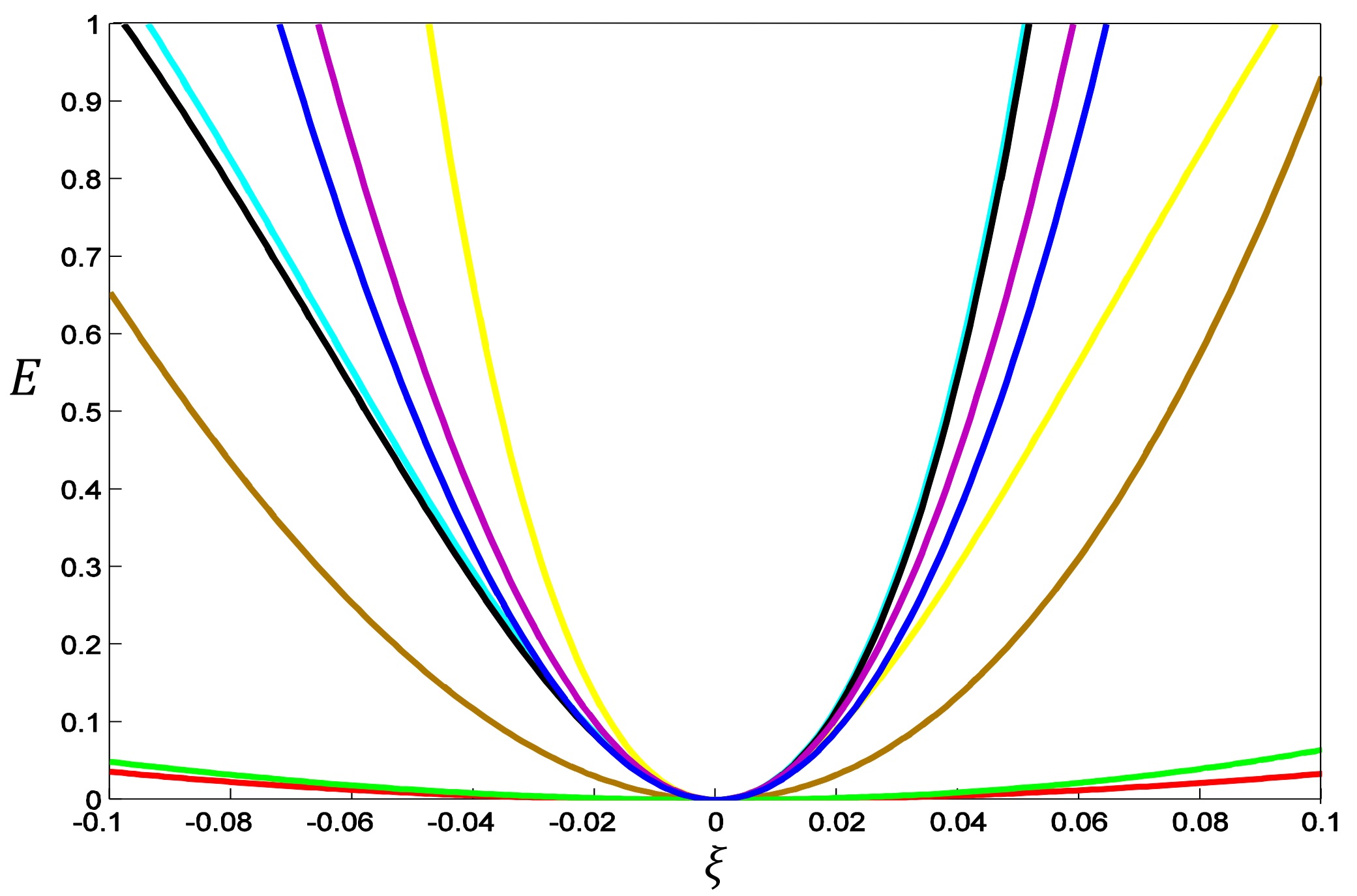
Figure 1: Variations of the total energy $E$ versus small $\xi$ for different deformations (34)-(41) at $t=0$. Various color curves of cyan, black, red, yellow, brown, purple, green and blue are related to various deformations (34)-(41), respectively.

Due to relativity, no particle can move faster than the speed of light, and therefore this massless particle (30), if it is considered a rigid body, will respond to any amount of force (interaction), no matter how tiny, by immediately accelerating to the speed of light. But, since the special solution (30) is a composite of two deformable fields $R$ and $\theta$ (as its internal structure), and then is not essentially a rigid body, it would be deformed ($R=R_{s}+\delta R$ and $\theta=\theta_{s}+\delta\theta$) in collisions or in interactions with other particles. In other words, it is not actually possible to perceive it as a rigid object with absolute zero rest mass. In fact, Heisenberg’s uncertainty principle essentially does not let us to have an ideal state for which the energy is absolute zero, and this statement is also valid for the special particle-like solution (30). Hence, physically, the particle-like solution (30) is always slightly deformed and then its rest mass is not absolute zero but it is very small, i.e. it is a stable soliton solution, which moves at a speed very close to the speed of light, but not exactly equal to the speed of light.

To establish an extended KG model (15) for which the stability of the single non-trivial solitary wave solution (30) is guaranteed appreciably through a simple and straightforward conclusion, we select three independent linear combinations of ${\cal S}_{ij}$’s in relations (16), (17) and (18) for which the functional coefficients $C_{i}$ ($i=1,2,3$) would be definitely positive and finally lead to a positive definite energy density function (21). In general, it may be possible to choose other combinations of ${\cal S}_{ij}$ for this goal. However, we intentionally introduced these special combinations as a good example of the extended KG systems for better and simpler conclusions.

IV Summary and conclusion

We have introduced, after reviewing some basic relations and equations of the standard relativistic classical field theory, the (nonlinear) KG and the extended KG systems for the scalar fields $\phi_{i}$. The Lagrangian density of a (nonlinear) KG system is linear in the kinetic scalar terms ${\cal S}_{ij}={\cal S}_{ji}=\partial_{\mu}\phi_{i}\partial^{\mu}\phi_{j}$. If the Lagrangian density of the scalar fields is not linear in the kinetic scalar terms, it can be called an extended KG system.

In this paper, it was shown that for a special example of the extended KG systems (15), there is a single non-trivial localized solitary wave solution with zero rest mass (30). The energy density function of this special extended KG system is bounded from below by zero. Therefore, the single solitary wave solution (30) has the minimum energy among the other solutions, i.e. it is really a massless stable localized solution. In other words, it is a zero rest mass soliton solution. The other unknown solutions of this system, undoubtedly, have non-zero positive rest energies.

The single massless soliton solution (30), if considered a rigid body, responds to any amount of force, no matter how tiny, by immediately accelerating to the speed of light. Therefore, since there is no area in the space with zero interaction, it has to move at the speed of light exactly according to the special relativity. But, since the stable zero rest mass solution (30) has internal structure and is not essentially a rigid body, it would be deformed in collisions or in interactions with other particles. Hence, it is not physically possible to perceive it as an absolute zero rest energy (mass) object. In fact, the zero rest mass soliton solution (30) is just an ideal mathematical solution, which can be considered in a free space without any other particles and interactions, but is not an interesting physical case. Hence, physically, the deformed soliton solution (30) can move at a speed very close to the speed of light, but not exactly equal to the speed of light.

References

- (1) Rajaraman R 1982 Solitons and Instantons (Amsterdam: North Holland, Elsevier)
- (2) Das A 1989 Integrable Models (Singapore: World Scientific)
- (3) Lamb G L Jr 1980 Elements of Soliton Theory (New York: Wiley-Interscience)
- (4) Drazin P G, Johnson R S 1989 Solitons: An Introduction (Cambridge: Cambridge University Press)
- (5) Campbell D K, Peyrard M 1986 Physica D 19 165 10.1016/0167-2789(86)90019-9
- (6) Campbell D K, Peyrard M 1986 Physica D 18 47 10.1016/0167-2789(86)90161-2
- (7) Campbell D K, Schonfeld J S, Wingate C A 1983 Physica D 9 1 10.1016/0167-2789(83)90289-0
- (8) Peyrard M, Campbell D K 1983 Physica D 9 33 10.1016/0167-2789(83)90290-7
- (9) Goodman R H, Haberman R 2005 SIAM J. Appl. Dyn. Syst. 4 1195 10.1137/050632981
- (10) Charkina O V, Bogdan M M, Verkin B I 2006 Symmetry. Integr. Geom. 2 047 10.3842/SIGMA.2006.047
- (11) Gharaati A R, Riazi N, Mohebbi F 2006 Int. J. Theor. Phys. 45 53 10.1007/s10773-005-9009-8
- (12) Mohammadi M, Riazi N 2011 Prog. Theor. Phys. 126 237 10.1143/PTP.126.237
- (13) Mohammadi M, Riazi N 2019 Commun. Nonlinear. Sci. Numer. Simulat. 72 176–193 10.1016/j.cnsns.2018.12.014
- (14) Hoseinmardi S, Riazi N 2010 Int. J. Mod. Phys. A 25 3261 10.1142/S0217751X10049712
- (15) Gani V A, Kudryavtsev A E 1999 Phys. Rev. E 60 3305 10.1103/PhysRevE.60.3305
- (16) Popov C A 2006 Wave Motion 42 309 10.1016/j.wavemoti.2005.04.007
- (17) Peyravi M, Montakhab A, Riazi N, Gharaati A 2009 Eur. Phys. J. B 72 269 10.1140/epjb/e2009-00331-0
- (18) Mohammadi M, Riazi N, Azizi A 2012 Prog. Theor. Phys. 128 615 10.1143/PTP.128.615
- (19) Wazwaz A M 2006 Chaos Solitons Fractals 28 1005 10.1016/j.chaos.2005.08.145
- (20) Dorey P, Mersh K, Romanczukiewicz T, Shnir Y 2011 Phys. Rev. Lett. 107 091602 10.1103/PhysRevLett.107.091602
- (21) Gani V A, Kudryavtsev A E, Lizunova M A 2014 Phys. Rev. D 89 125009 10.1103/PhysRevD.89.125009
- (22) Khare A, Christov I C, Saxena A 2014 Phys. Rev. E 90 023208 10.1103/PhysRevE.90.023208
- (23) Moradi Marjaneh A, Gani V A, Saadatmand D 2017 J. High Energy Phys. 2017 1 10.1007/JHEP07(2017)028
- (24) Bazeia D, Belendryasova E, Gani V A 2018 Eur. Phys. J. C 78 340 10.1140/epjc/s10052-018-5815-z
- (25) Gani V A et al. 2018 Eur. Phys. J. C 78 345 10.1140/epjc/s10052-018-5813-1
- (26) Doreya P, Romańczukiewicz T 2018 Phys. Lett. B 779 117–23 10.1016/j.physletb.2018.02.003
- (27) Panin A G, Smolyakov M N 2017 Phys. Rev. D 95 065006 10.1103/PhysRevD.95.065006
- (28) Kovtun A, Nugaev E, Shkerin A 2018 Phys. Rev. D 98 096016 10.1103/PhysRevD.98.096016
- (29) Smolyakov M N 2018 Phys. Rev. D 97 045011 10.1103/PhysRevD.97.045011
- (30) Tsumagari M I, Copeland E J, Saffin P M 2008 Phys. Rev. D 78 065021 10.1103/PhysRevD.78.065021
- (31) Lee T D, Pang Y 1992 Phys. Rep. 221 251 10.1016/0370-1573(92)90064-7
- (32) Coleman S 1985 Nucl. Phys. B 262 263 10.1016/0550-3213(85)90286-X
- (33) Bazeia D, Marques M A, Menezes R 2016 Eur. Phys. J. C 76 241 10.1140/epjc/s10052-016-4059-z
- (34) Bazeia D et al. 2017 Phys. Lett. B 765 359 10.1016/j.physletb.2016.12.033
- (35) Anagnostopoulos K N et al. 2001 Phys. Rev. D 64 125006 10.1103/PhysRevD.64.125006
- (36) Axenides M et al. 2000 Phys. Rev. D 61 085006 10.1103/PhysRevD.61.085006
- (37) Bowcock P, Foster D, Sutcliffe P 2009 J. Phys. A: Math. Theor. 42 085403 10.1088/1751-8113/42/8/085403
- (38) Shiromizu T, Uesugi T, Aoki M 1999 Phys. Rev. D 59 125010 10.1103/PhysRevD.59.125010
- (39) Shiromizu T 1998 Phys. Rev. D 58 10 730110.1103/PhysRevD.58.107301
- (40) Bazeia D et al. 2016 Phys. Lett. B 758 146–151 10.1016/j.physletb.2016.04.060
- (41) Riazi N 2011 Int. J. Theor. Phys. 50 3451 10.1007/s10773-011-0850-7
- (42) Mohammadi M, Riazi N 2014 Prog. Theor. Exp. Phys. 2014 023A03 10.1093/ptep/ptu002
- (43) Skyrme T H R 1961 Proc. Roy. Soc. A 260 127 10.1098/rspa.1961.0018
- (44) Wong S M H 2002 arXiv:hep-ph/0202250v2
- (45) ’t Hooft G 1974 Nucl. Phys. B 79 276 10.1016/0550-3213(74)90486-6
- (46) Polyakov A M 1974 JETP Lett. 20 194