On Symmetric Losses for Learning from Corrupted Labels

Abstract

This paper aims to provide a better understanding of a symmetric loss. First, we emphasize that using a symmetric loss is advantageous in the balanced error rate (BER) minimization and area under the receiver operating characteristic curve (AUC) maximization from corrupted labels. Second, we prove general theoretical properties of symmetric losses, including a classification-calibration condition, excess risk bound, conditional risk minimizer, and AUC-consistency condition. Third, since all nonnegative symmetric losses are non-convex, we propose a convex barrier hinge loss that benefits significantly from the symmetric condition, although it is not symmetric everywhere. Finally, we conduct experiments to validate the relevance of the symmetric condition.

1 Introduction

In the real-world, it is unrealistic to expect that clean fully-supervised data can always be obtained. Weakly-supervised learning is a learning paradigm to mitigate this problem (Zhou, 2017). For example, labelers are not necessarily experts or even human experts can make mistakes. Learning under noisy labels is an example of weakly-supervised learning that relaxes the assumption that labels are always accurate (Aslam & Decatur, 1996; Biggio et al., 2011; Cesa-Bianchi et al., 1999; Natarajan et al., 2013). Other examples of weakly-supervised learning are learning from positive and unlabeled data (du Plessis et al., 2015, 2014; Kiryo et al., 2017), learning from pairwise similarity and unlabeled data (Bao et al., 2018), and learning from complementary labels (Ishida et al., 2017).

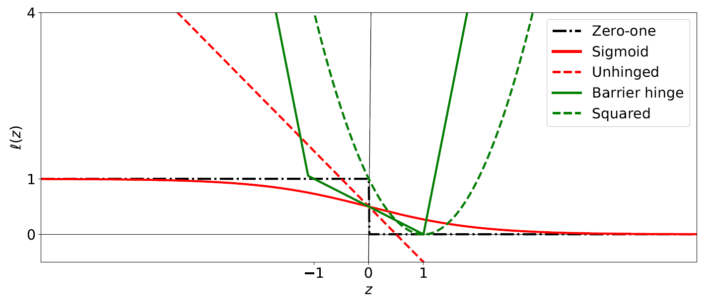
Figure 1: Examples of losses used in this paper. The zero-one loss, sigmoid loss, and unhinged loss are symmetric, i.e., $\ell(z)+\ell(-z)$ is a constant. The barrier hinge loss is our proposed loss.

A loss function that satisfies a symmetric condition has demonstrated its usefulness in weakly-supervised learning, e.g., one can use a symmetric loss to simplify a risk estimator in learning from positive-unlabeled data (du Plessis et al., 2014). This simplification allows the use of a cost-sensitive learning library to implement the risk estimator directly. Not limited to the simplification of the risk estimator, symmetric losses are known to be robust in the symmetric label noise scenarios (Manwani & Sastry, 2013; Ghosh et al., 2015). However, the symmetric label noise assumption is restrictive and may not be practical since it assumes that a label of each pattern may flip independently with the same probability.

This paper elucidates the robustness of symmetric losses in a more general noise framework called the mutually contaminated distributions or corrupted labels framework (Scott et al., 2013). Many weakly-supervised learning problems can be formulated in the corrupted labels framework (Natarajan et al., 2013; Lu et al., 2018). Therefore, the robustness of learning from corrupted labels is highly desirable for many real-world applications.

Although it has been shown by Menon et al. (2015) that BER and AUC optimization from corrupted labels can be optimized without knowing the noise information, we point out that the use of non-symmetric losses may degrade the performance and therefore using a symmetric losses is preferable. Our experiments show that symmetric losses significantly outperformed many well-known non-symmetric losses when the given labels are corrupted. Furthermore, we provide a better understanding of symmetric losses by elucidating several general theoretical properties of symmetric losses, including a classification-calibration condition, excess risk bound, conditional risk minimizer, and AUC-consistency. We show that many well-known symmetric losses are suitable for both classification and bipartite ranking problems. We also discuss the negative result of symmetric losses, which is the inability to recover the class probability given the risk minimizer. This suggests a limitation to use such symmetric losses for a task that requires a prediction confidence such as learning with a reject option (Chow, 1970; Yuan & Wegkamp, 2010).

Unfortunately, it is known that a nonnegative symmetric loss must be non-convex (du Plessis et al., 2014; Ghosh et al., 2015).  van Rooyen et al. (2015a) proposed an unhinged loss, which is convex, symmetric but negatively unbounded. In this paper, we propose a barrier hinge loss which is convex, nonnegative, and satisfies the symmetric condition in a subset of the domain space, not everywhere.

2 Preliminaries

In this section, we review the notation and related work of symmetric losses and learning from corrupted labels.

2.1 Notation

Let $\boldsymbol{x}\in\mathbb{R}^{d}$ be a $d$-dimensional real-valued pattern, $y\in\{-1,+1\}$ denote a class label which can only be either positive or negative, and $g\colon\mathbb{R}^{d}\to\mathbb{R}$ denote a prediction function. In binary classification, we use sign$(g(\boldsymbol{x}))$ to determine the predicted label of a prediction function, where sign$(g(\boldsymbol{x}))=1$ if $g(\boldsymbol{x})>0$, $-1$ if $g(\boldsymbol{x})<0$, and $0$ otherwise. $\mathbb{E}_{\mathrm{P}}[\cdot]$ and $\mathbb{E}_{\mathrm{N}}[\cdot]$ denote the expectations of $\boldsymbol{x}$ over $p(\boldsymbol{x}|y=1)$ and $p(\boldsymbol{x}|y=-1)$, respectively. $\eta(\boldsymbol{x})$ indicates the class probability $p(y=1|\boldsymbol{x})$ of a pattern $\boldsymbol{x}$. In this paper, we consider a margin loss $\ell\colon\mathbb{R}\to\mathbb{R}$ that takes only one argument, which is typically $yg(\boldsymbol{x})$. Table 1 shows examples of margin losses.

2.2 Symmetric Losses

Note that the notion of a symmetric loss can be ambiguous since there are many definitions of symmetric loss (see  Natarajan et al. (2013); Reid & Williamson (2010) for other definitions). In this paper, we consider a symmetric loss from the perspective that it is a margin loss, $\ell\colon\mathbb{R}\to\mathbb{R}$ that satisfies the symmetric condition, i.e., $\ell(z)+\ell(-z)=K$, where $K$ is a constant. Examples of such losses are the zero-one loss, unhinged loss and sigmoid loss which are described in Figure 1.

The advantage of using a symmetric loss was investigated in the symmetric label noise scenario (Manwani & Sastry, 2013; Ghosh et al., 2015; van Rooyen et al., 2015a). The results from  Long & Servedio (2010) suggested that convex losses are non-robust in this scenario and this motivated the use of a robust non-convex loss in the symmetric label noise scenario. Ghosh et al. (2015) proved that the symmetric condition is sufficient for a loss to be robust in this scenario.  van Rooyen et al. (2015a) later proposed an unhinged loss, which is the only possible convex loss to be symmetric, but it needs to be negatively unbounded. The negative unboundedness is not a common property for a loss function, which avoids the condition in Long & Servedio (2010) to achieve the robustness in the symmetric label noise scenario. Another notable extension of a symmetric condition is the extension to a multiclass setting (Ghosh et al., 2017).

This paper considers a noise framework called mutually contaminated distributions or corrupted labels framework (Scott et al., 2013), where the symmetric label noise is a special case of the corrupted labels framework (Menon et al., 2015). Then, we discuss a problem of non-symmetric losses in this scenario and emphasize that advantage of symmetric losses.

2.3 Learning from Corrupted Labels

In the corrupted labels scenario, we are given two sets of data drawn from the corrupted positive and corrupted negative marginal distributions respectively as follows:

$$\{\boldsymbol{x}_{i}\}_{i=1}^{n_{\mathrm{CP}}} \stackrel{{\scriptstyle\mathrm{i.i.d.}}}{{\sim}}\pi p(\boldsymbol{x}|y=1)+(1-\pi)p(\boldsymbol{x}|y=-1)\text{,}$$

$$\{\boldsymbol{x}_{j}\}_{j=1}^{n_{\mathrm{CN}}} \stackrel{{\scriptstyle\mathrm{i.i.d.}}}{{\sim}}\pi^{\prime}p(\boldsymbol{x}|y=1)+(1-\pi^{\prime})p(\boldsymbol{x}|y=-1)\text{,}$$

where $n_{\mathrm{CP}}$ denotes the number of corrupted positive patterns and $\pi$ is the class prior $p(y=1)$ for the corrupted positive distribution, i.e, a proportion of clean positive data in the corrupted positive data. $n_{\mathrm{CN}}$ and $\pi^{\prime}$ are defined similarly for the corrupted negative data. We denote $X_{\mathrm{CP}}:=\{\boldsymbol{x}_{i}\}_{i=1}^{n_{\mathrm{CP}}}$ as a corrupted positive sample and $X_{\mathrm{CN}}:=\{\boldsymbol{x}_{j}\}_{j=1}^{n_{\mathrm{CN}}}$ as a corrupted negative sample. $p(\boldsymbol{x}|y)$ denotes the class conditional density. In this setting, $\pi\neq\pi^{\prime}$ but the class condition probabilities $p(\boldsymbol{x}|y)$ are identical for both sets. Clean data implies $\pi=1,\pi^{\prime}=0$. The class prior in this case can also be interpreted as the noise rate (Menon et al., 2015), where $(1-\pi)$ is the noise rate for positive data and $\pi^{\prime}$ is the noise rate for negative data. We assume $\pi>\pi^{\prime}$ for simplicity. Otherwise, labels from the classifier must be flipped.

Menon et al. (2015) first showed that BER and AUC optimization from corrupted labels yield the same minimizer as minimizing from the clean labels. However, in this paper, we take a closer look of this problem and point out that the use of surrogate losses may yield different minimizers and degrade the performance. Another notable work in this corrupted labels setting is the classification from two sets of unlabeled data (Lu et al., 2018). They proposed an unbiased risk estimator for the classification error metric in this setting. BER is a special case of the classification error metric where the class prior is balanced. Nevertheless, their unbiased risk estimator requires the knowledge of the class priors of the two training distributions and the test distribution. This paper only focuses on BER and AUC optimization and does not require any class prior information.

3 The Importance of Symmetric Losses in BER and AUC Optimization

In this section, we show that using a symmetric loss is preferable for BER and AUC optimization from corrupted labels without class prior estimation. BER and AUC are popular metrics for imbalanced data classification (Cheng et al., 2002; Guyon et al., 2005). Furthermore, AUC is also known as an evaluation metric for bipartite ranking (Narasimhan & Agarwal, 2013; Menon & Williamson, 2016). In the corrupted labels framework, the class prior estimation problem is known to be a bottleneck in this framework since it is an unidentifiable problem unless a restrictive condition is applied (Blanchard et al., 2010; Scott, 2015). Thus, being able to minimize BER and AUC without estimating class priors is a great advantage in practice.

Related work: Menon et al. (2015) proved that for the zero-one loss, the clean and corrupted BER/AUC risks have the same minimizer. However, it remains unclear whether the same result holds for any surrogate losses. Later, van Rooyen et al. (2015b) generalized the result of BER minimization in Menon et al. (2015) from the zero-one loss to any symmetric losses. In this paper, we analyze both BER and AUC optimization from corrupted labels by first proving the relationship between the clean surrogate risk and corrupted surrogate risk for any surrogate losses. Our results indicate that using a non-symmetric loss may not yield the same minimizer for the clean and corrupted risks since it may suffer from excessive terms (see Sections 3.1 and 3.2). Then, we clarify that similarly to BER minimization that was proven by van Rooyen et al. (2015b), using a symmetric loss is also advantageous for AUC maximization. We are also the first to provide the experimental results for validating the advantage of symmetric losses for BER and AUC optimization from corrupted labels in practice.

3.1 Area under the Receiver Operating Characteristic Curve (AUC) Maximization

In AUC maximization, we consider the following AUC risk (Narasimhan & Agarwal, 2013):

$$R^{\ell}_{\mathrm{AUC}}(g)=\mathbb{E}_{\mathrm{P}}[\mathbb{E}_{\mathrm{N}}[\ell(f(\boldsymbol{x}_{\mathrm{P}},\boldsymbol{x}_{\mathrm{N}}))]]\text{,}$$ (1)

where $f(\boldsymbol{x},\boldsymbol{x}^{\prime})=g(\boldsymbol{x})-g(\boldsymbol{x}^{\prime})$. The expected AUC score is $1-R^{\ell_{0\text{-}1}}_{\mathrm{AUC}}(g)$. Therefore, we can maximize the AUC score by minimizing the AUC risk. Since we do not have access to clean data, let us consider a corrupted AUC risk with a surrogate loss $\ell$ that treats $X_{\mathrm{CP}}$ as being positive and $X_{\mathrm{CN}}$ as being negative:

$$R^{\ell}_{\mathrm{AUC}\text{-}\mathrm{Corr}}(g)=\mathbb{E}_{\mathrm{CP}}[\mathbb{E}_{\mathrm{CN}}[\ell(f(\boldsymbol{x}_{\mathrm{CP}},\boldsymbol{x}_{\mathrm{CN}}))]]\text{.}$$

The following theorem shows that by using a symmetric loss, the minimizers of $R^{\ell}_{\mathrm{AUC}\text{-}\mathrm{Corr}}(g)$ and $R^{\ell}_{\mathrm{AUC}}(g)$ are identical (its proof is given in Appendix).

Theorem 1.

Let $\gamma^{\ell}(\boldsymbol{x},\boldsymbol{x}^{\prime})=\ell(f(\boldsymbol{x}^{\prime},\boldsymbol{x}))+\ell(f(\boldsymbol{x},\boldsymbol{x}^{\prime}))$. Then $R^{\ell}_{\mathrm{AUC}\text{-}\mathrm{Corr}}(g)$ can be expressed as

$$\begin{split}R^{\ell}_{\mathrm{AUC}\text{-}\mathrm{Corr}}(g)={}&(\pi-\pi^{\prime})R^{\ell}_{\mathrm{AUC}}(g)\\ &+\underbrace{(1-\pi)\pi^{\prime}\mathbb{E}_{\mathrm{P}}[\mathbb{E}_{\mathrm{N}}[\gamma^{\ell}(\boldsymbol{x}_{\mathrm{P}},\boldsymbol{x}_{\mathrm{N}})]]}_{\textup{Excessive term}}\\ &+\underbrace{\frac{\pi\pi^{\prime}}{2}\mathbb{E}_{\mathrm{P^{\prime}}}[\mathbb{E}_{\mathrm{P}}[\gamma^{\ell}(\boldsymbol{x}_{\mathrm{P^{\prime}}},\boldsymbol{x}_{\mathrm{P}})]]}_{\textup{Excessive term}}\\ &+\underbrace{\frac{(1-\pi)(1-\pi^{\prime})}{2}\mathbb{E}_{\mathrm{N^{\prime}}}[\mathbb{E}_{\mathrm{N}}[\gamma^{\ell}(\boldsymbol{x}_{\mathrm{N^{\prime}}},\boldsymbol{x}_{\mathrm{N}})]]}_{\textup{Excessive term}}\text{.}\end{split}$$

Corollary 2.

Let $\ell$ be a symmetric loss such that $\ell(z)+\ell(-z)=K$, where $K$ is a constant. $R^{\ell}_{\mathrm{AUC}\text{-}\mathrm{Corr}}(g)$ can be expressed as

$$R^{\ell}_{\mathrm{AUC}\text{-}\mathrm{Corr}}(g)=(\pi-\pi^{\prime})R^{\ell}_{\mathrm{AUC}}(g)+K\left(\frac{1-\pi+\pi^{\prime}}{2}\right)\text{.}$$

Corollary 2 can be obtained simply by substituting $\gamma^{\ell}(\boldsymbol{x},\boldsymbol{x}^{\prime})$ with $K$. This suggests that the excessive term becomes a constant when using a symmetric loss and guarantees that the minimizers of $R^{\ell}_{\mathrm{AUC}\text{-}\mathrm{Corr}}(g)$ and $R^{\ell}_{\mathrm{AUC}}(g)$ are identical. On the other hand, if a loss is non-symmetric, then the excessive terms are not constants and the minimizers of both risks may differ. A special case of this setting where $\pi=1$ has been studied by Sakai et al. (2018). They showed that a convex surrogate loss can be applied but $\pi^{\prime}$ needs to be estimated in order to cancel the excessive term. By using a symmetric loss, the class prior estimation is not required and the given positive patterns can also be corrupted. More generally, our results indicate that using a symmetric loss for AUC maximization from corrupted labels yields the same minimizer as clean labels and can be applied to various weakly-supervised learning settings (Natarajan et al., 2013; Niu et al., 2016; Bao et al., 2018; Lu et al., 2018).

3.2 Balanced Error Rate (BER) Minimization

Consider the following misclassification risk:

$$R^{\ell}_{\mathrm{BER}}(g) =\frac{1}{2}\left[\mathbb{E}_{\mathrm{P}}\left[\ell(g(\boldsymbol{x}))\right]+\mathbb{E}_{\mathrm{N}}\left[\ell(-g(\boldsymbol{x}))\right]\right]\text{.}$$

The BER minimization problem is equivalent to minimizing $R^{\ell_{0\text{-}1}}_{\mathrm{BER}}(g)$. i.e., the classification risk with the zero-one loss when the class prior of the test distribution is balanced.

Let us define

$$R^{\ell}_{\mathrm{BER}\text{-}\mathrm{Corr}}(g)=\frac{1}{2}\big{[}R_{\mathrm{CP}}^{\ell}(g)+R_{\mathrm{CN}}^{\ell}(g)\big{]}\text{,}$$

where

$$R_{\mathrm{CP}}^{\ell}(g) =\pi\mathbb{E}_{\mathrm{P}}[\ell(g(\boldsymbol{x}))]+(1-\pi)\mathbb{E}_{\mathrm{N}}[\ell(g(\boldsymbol{x}))]\text{,}$$

$$R_{\mathrm{CN}}^{\ell}(g) =\pi^{\prime}\mathbb{E}_{\mathrm{P}}[\ell(-g(\boldsymbol{x}))]+(1-\pi^{\prime})\mathbb{E}_{\mathrm{N}}[\ell(-g(\boldsymbol{x}))]\text{.}$$

Then, we state the following theorem (its proof is given in Appendix).

Theorem 3.

Let $\gamma^{\ell}(\boldsymbol{x})=\ell(g(\boldsymbol{x}))+\ell(-g(\boldsymbol{x}))$, $R^{\ell}_{\mathrm{BER}\text{-}\mathrm{Corr}}(g)$ can be expressed as

$$R^{\ell}_{\mathrm{BER}\text{-}\mathrm{Corr}}(g) =(\pi-\pi^{\prime}){R^{\ell}_{\mathrm{BER}}(g)}$$

$$\quad+\underbrace{\frac{\pi^{\prime}\mathbb{E}_{\mathrm{P}}[\gamma^{\ell}(\boldsymbol{x})]+(1-\pi)\mathbb{E}_{\mathrm{N}}[\gamma^{\ell}(\boldsymbol{x})]}{2}}_{\textup{Excessive term}}\text{.}$$

By observing an excessive term, we can directly obtain the following corollary, which coincides with the existing result by van Rooyen et al. (2015b).

Corollary 4 (van Rooyen et al. (2015b)).

Let $\ell$ be a symmetric loss such that $\ell(z)+\ell(-z)=K$, where $K$ is a constant. $R^{\ell}_{\mathrm{BER}\text{-}\mathrm{Corr}}(g)$ can be expressed as

$$R^{\ell}_{\mathrm{BER}\text{-}\mathrm{Corr}}(g)=(\pi-\pi^{\prime})R^{\ell}_{\mathrm{BER}}(g)+K\left(\frac{1-\pi+\pi^{\prime}}{2}\right)\text{.}$$

Similarly to Corollary 2, if a loss $\ell$ is symmetric, then the excessive term is a constant and the minimizers of $R^{\ell}_{\mathrm{BER}\text{-}\mathrm{Corr}}(g)$ and $R^{\ell}_{\mathrm{BER}}(g)$ are guaranteed to be identical.

Table 1: Loss functions and their properties including the convexity, symmetricity, capability of recovering $\eta(\boldsymbol{x})$, and their conditional risk minimizers $f^{\ell*}(\boldsymbol{x})$. Although the conditional risk minimizers of each loss function are different, the sign of each minimizer sign$(f^{\ell*}(\boldsymbol{x}))$ matches each other, which agrees with the Bayes-optimal classifier. The savage loss is proposed by Masnadi-Shirazi & Vasconcelos (2009). The minimizer $f^{\ell*}(\boldsymbol{x})$ of the ramp, sigmoid, and unhinged losses are unique if the prediction output is in $[-1,1]$.

Loss name	$\ell(z)$	$f^{\ell*}(\boldsymbol{x})$	Convex	Symmetric	Recover $\eta(\boldsymbol{x})$
Zero-one	$-0.5\mathrm{sign}(z)+0.5$	$\mathrm{sign}(\eta(\boldsymbol{x})-0.5)$	$\times$	$\checkmark$	$\times$
Squared	$(1-z)^{2}$	$2\eta(\boldsymbol{x})-1$	$\checkmark$	$\times$	$\checkmark$
Hinge	$\max(0,1-z)$	$\mathrm{sign}(\eta(\boldsymbol{x})-0.5)$	$\checkmark$	$\times$	$\times$
Logistic	$\mathrm{log}(1+\exp(-z))$	$\mathrm{log}\left(\frac{\eta(\boldsymbol{x})}{1-\eta(\boldsymbol{x})}\right)$	$\checkmark$	$\times$	$\checkmark$
Savage	$\left[(1+\exp(2z))^{2}\right]^{-1}$	$0.5\mathrm{log}\left(\frac{\eta(\boldsymbol{x})}{1-\eta(\boldsymbol{x})}\right)$	$\times$	$\times$	$\checkmark$
Ramp	$\mathrm{max}(0,\mathrm{min}(1,0.5-0.5z))$	$\mathrm{sign}(\eta(\boldsymbol{x})-0.5)$	$\times$	$\checkmark$	$\times$
Sigmoid	$\left[1+\exp(z)\right]^{-1}$	$\mathrm{sign}(\eta(\boldsymbol{x})-0.5)$	$\times$	$\checkmark$	$\times$
Unhinged	$1-z$	$\mathrm{sign}(\eta(\boldsymbol{x})-0.5)$	$\checkmark$	$\checkmark$	$\times$

4 Theoretical Properties of Symmetric Losses

In this section, we investigate general theoretical properties of symmetric losses. Since all nonnegative symmetric losses are non-convex, many convenient conditions that assume a loss function is convex cannot be applied (Zhang, 2004; Bartlett et al., 2006; Gao & Zhou, 2015; Niu et al., 2016). Nevertheless, thanks to the symmetric condition, we show that it is possible to derive general theoretical properties of a symmetric loss.

4.1 Classification-calibration

The main motivation to use a surrogate loss in binary classification is that the zero-one loss is discontinuous and therefore difficult to optimize (Ben-David et al., 2003; Feldman et al., 2012). A natural question is what kind of surrogate losses can be used instead of the zero-one loss. This problem has been studied extensively in binary classification (Zhang, 2004; Bartlett et al., 2006). Classification-calibration is known to be a minimal requirement of a loss function for the binary classification task (see  Bartlett et al. (2006) for more details on classification-calibration).

We derive the following theorem that establishes a necessary and sufficient condition for a symmetric loss to be classification-calibrated (its proof is given in Appendix).

Theorem 5.

A symmetric loss $\ell\colon\mathbb{R}\to\mathbb{R}$ such that $\ell(z)+\ell(-z)$ is a constant is classification-calibrated if and only if $\inf\limits_{\alpha>0}\ell(\alpha)<\inf\limits_{\alpha\leq 0}\ell(\alpha)$.

The following corollary is straightforward from the theorem above, but we emphasize it since it covers many surrogate symmetric losses, e.g., the sigmoid, ramp, and unhinged losses.

Corollary 6.

A non-increasing loss $\ell\colon\mathbb{R}\to\mathbb{R}$ such that $\ell(z)+\ell(-z)$ is a constant and $\ell^{\prime}(0)<0$, is classification-calibrated.

Based on Theorem 5, by simply checking the condition whether $\inf\limits_{\alpha>0}\ell(\alpha)<\inf\limits_{\alpha\leq 0}\ell(\alpha)$ is necessary and sufficient to determine if a symmetric loss is classification-calibrated. Note that Corollary 6 is a sufficient condition that covers many symmetric losses such as the ramp loss and sigmoid loss. In general, the differentiability at zero of a symmetric loss is not required to verify the classification-calibrated condition unlike convex losses (Bartlett et al., 2006). Note that some specific symmetric losses such as the ramp loss and sigmoid loss were proven to be classification-calibrated (Bartlett et al., 2006; Niu et al., 2016). This paper provides a necessary and sufficient condition for all symmetric losses.

4.2 Excess Risk Bound

The excess risk bound provides a relationship between the excess risk of minimizing the misclassification risk with respect to the zero-one loss and the surrogate loss. It is known that an excess risk bound of a loss $\ell$ exists if and only if $\ell$ is classification-calibrated (Bartlett et al., 2006).

Consider the standard binary misclassification risk:

$$R^{\ell}(g)=\mathop{\mathbb{E}}\limits_{(\boldsymbol{x},y)\sim D}\left[\ell(yg(\boldsymbol{x}))\right]\text{.}$$ (2)

The following theorem indicates an excess risk bound for any classification-calibrated symmetric loss (its proof is given in Appendix).

Theorem 7.

An excess risk bound of a classification-calibrated symmetric loss $\ell\colon\mathbb{R}\to\mathbb{R}$ such that $\ell(z)+\ell(-z)$ is a constant can be expressed as

$$R^{\ell_{0\text{-}1}}(g)-R^{\ell_{0\text{-}1}*} \leq\frac{R^{\ell}(g)-R^{\ell*}}{\inf\limits_{\alpha\leq 0}\ell(\alpha)-\inf\limits_{\alpha>0}\ell(\alpha)}\text{,}$$

where $R^{\ell*}=\inf\limits_{g}R^{\ell}(g)$ and $R^{\ell_{0\text{-}1}*}=\inf\limits_{g}R^{\ell_{0\text{-}1}}(g)$.

The result suggests that the excess risk bound of any classification-calibrated symmetric loss is controlled only by the difference of the infima $\inf\limits_{\alpha>0}\ell(\alpha)-\inf\limits_{\alpha\leq 0}\ell(\alpha)$. Intuitively, the excess risk bound tells us that if the prediction function $g$ minimizes the surrogate risk $R^{\ell}(g)=R^{\ell*}$, then the prediction function $g$ must also minimize the misclassification risk $R^{\ell_{0\text{-}1}}(g)=R^{\ell_{0\text{-}1}*}$.

4.3 Inability to Recover the Class Probability $\eta(\boldsymbol{x})$

We investigate the form of the conditional risk minimizer of a symmetric loss. The conditional risk minimizer is useful to know the behavior of a prediction function learned from minimizing such a surrogate loss. For example, we can recover a class probability $\eta(\boldsymbol{x})$ from a prediction function if a loss $\ell$ is a proper composite loss (Buja et al., 2005; Reid & Williamson, 2010). The mapping function to recover a class probability $\eta(\boldsymbol{x})$ depends on the conditional risk minimizer. For example, one can recover the class probability $\eta(\boldsymbol{x})$ of the squared loss by the relationship $\eta(\boldsymbol{x})=\frac{f^{\ell_{\mathrm{sq}}*}(\boldsymbol{x})+1}{2}$. Table 1 shows the examples of classification-calibrated losses and their conditional risk minimizers.

Our following theorem states that the conditional risk minimizer of any classification-calibrated symmetric loss can be expressed as a scaled Bayes-optimal classifier (its proof is given in Appendix).

Theorem 8.

Let $\ell$ be a symmetric loss $\ell\colon\mathbb{R}\to\mathbb{R}$ such that $\ell(z)+\ell(-z)$ is a constant and classification-calibrated, if the minimum of $\ell$ exists and $M\in\operatorname*{arg\,min}\limits_{\alpha\in\mathbb{R}}\ell(\alpha)$. Then, the condition risk minimizer of $\ell$ can be expressed as follows:

$$f^{\ell*}(\boldsymbol{x})=M\,\mathrm{sign}(\eta(\boldsymbol{x})-\frac{1}{2})\text{,}$$

where $\eta(\boldsymbol{x})=p(y=1|\boldsymbol{x})$.

When a symmetric loss is classification-calibrated but the minimum does not exist, $M$ $\to$ $\infty$. Note that the minimizer of a symmetric loss does not need to be unique as there might exist many points that give the minimum value.

By observing the conditional risk minimizer in Theorem 8, it is obvious that the class probability $\eta(\boldsymbol{x})$ cannot be recovered from the conditional risk minimizer since it knows only whether $\eta(\boldsymbol{x})>\frac{1}{2}$. This similar property has been observed and well-studied for the hinge loss $\ell_{\mathrm{hinge}}(z)=\mathrm{max}(0,1-z)$, where its minimizer is the Bayes-optimal classifier $\mathrm{sign}(\eta(\boldsymbol{x})-\frac{1}{2})$, which suggests that the hinge loss is not suitable for class probability estimation (Bartlett & Tewari, 2007; Buja et al., 2005; Reid & Williamson, 2010).

4.4 AUC-consistency

AUC-consistency is similar to classification-calibration but from the perspective of AUC maximization (Gao & Zhou, 2015), i.e., minimizing the pairwise conditional risk for AUC maximization instead of the pointwise conditional risk in bainry classification. The Bayes-optimal solution of AUC maximization is a function that has a strictly monotonic relationship with the class probability $\eta(\boldsymbol{x})$, which is a consequence of the Neyman-Pearson lemma (Menon & Williamson, 2016).

Our following lemma states that classification-calibration is necessary for a symmetric loss to be AUC-consistent (its proof is given in Appendix).

Lemma 9.

An AUC consistent symmetric loss $\ell\colon\mathbb{R}\to\mathbb{R}$ such that $\ell(z)+\ell(-z)$ is a constant, is classification-calibrated.

Next, an interesting question is whether all classification-calibrated symmetric losses are AUC-consistency. We prove by giving a counterexample that unfortunately this is not the case (its proof is given in Appendix).

Proposition 10.

Classification-calibration is necessary yet insufficient for a symmetric loss $\ell\colon\mathbb{R}\to\mathbb{R}$ such that $\ell(z)+\ell(-z)$ to be AUC-consistent.

Proposition 10 illustrates that there is a gap between classification-calibration and AUC-consistency for a symmetric loss. This gives rise to an important question whether well-known symmetric losses are AUC-consistent. We elucidate the positive result by establishing a sufficient condition for a symmetric loss to be AUC-consistent, which covers almost all existing surrogate symmetric losses to the best of our knowledge (its proof is given in Appendix).

Theorem 11.

A non-increasing loss $\ell\colon\mathbb{R}\to\mathbb{R}$ such that $\ell(z)+\ell(-z)$ is a constant and $\ell^{\prime}(0)<0$, is AUC-consistent.

With Corollary 6 and Theorem 11, we show that a non-increasing symmetric loss that $\ell^{\prime}(0)<0$ is sufficient to be both classification-calibrated and AUC-consistent. Such conditions are not difficult to satisfy in practice. In fact, most surrogate symmetric losses that we are aware of satisfy this condition. Thus, the choice of symmetric losses is highly flexible for both the classification and bipartite ranking problems.

5 Barrier Hinge Loss

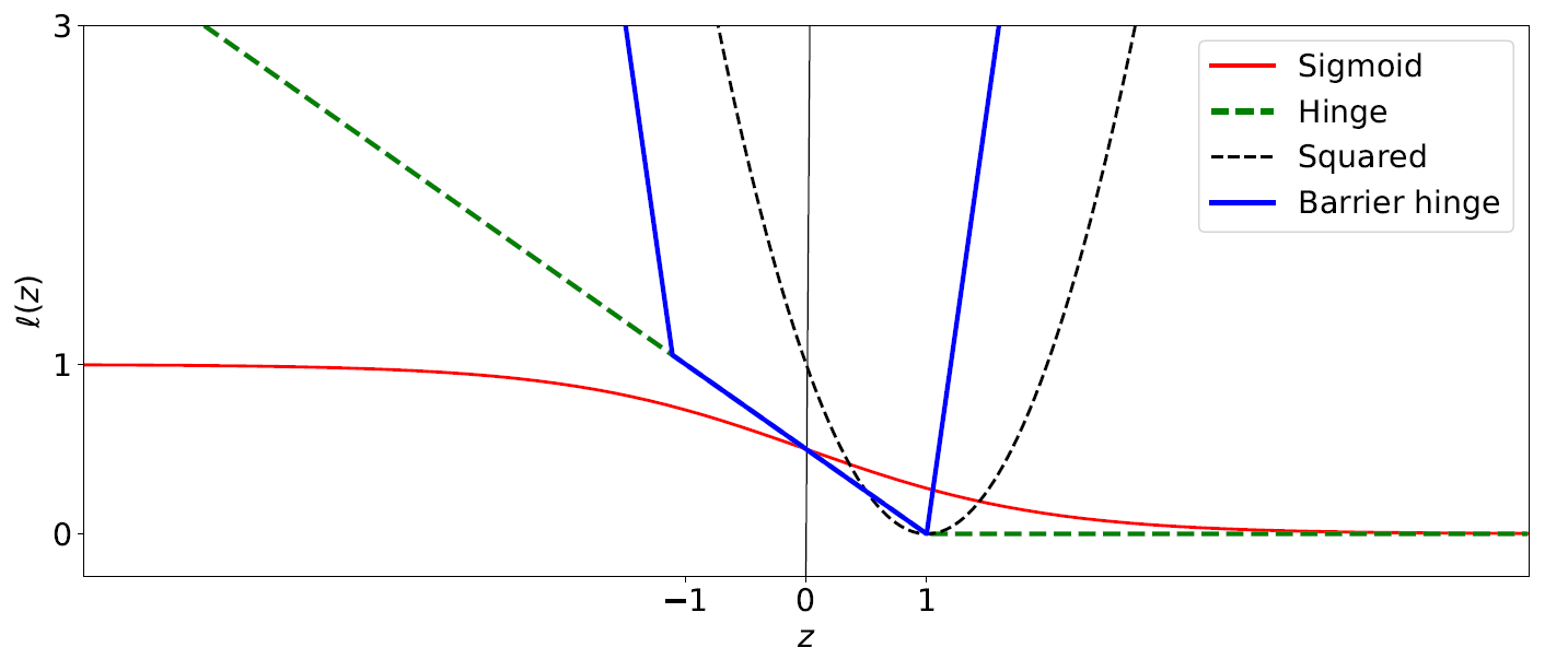
Figure 2: The barrier hinge loss scaled by $0.5$ with $b=10,r=1$: $\ell(z)=0.5\mathrm{max}(-10(1+z)+1,\mathrm{max}(10(z-1),1-z))$, the hinge loss: $\ell(z)=\mathrm{max}(0,0.5-0.5z)$ and the sigmoid loss: $\ell(z)=\left[1+\exp(z)\right]^{-1}$. The symmetric property holds for the barrier hinge loss for $z\in[-1,1]$.

In this section, we propose a convex loss that benefits from the symmetric condition although it is not symmetric everywhere. Note that it is impossible to have a nonnegative symmetric loss (du Plessis et al., 2014; Ghosh et al., 2015). Our main idea to compensate this problem is to construct a loss that does not have to satisfy the symmetric condition everywhere, i.e ., $\ell(z)+\ell(-z)$ is a constant for every $z\in\mathbb{R}$. In this case, it is possible to find a classification-calibrated convex loss function that satisfies the symmetric condition only for an interval in $\mathbb{R}$. For example, the hinge loss satisfies the symmetric condition for $z\in[-1,1]$. Nevertheless, the symmetric condition does not hold for $z$ when $z\notin[-1,1]$ and might suffer from the excessive term. Motivated by this observation, we propose a barrier hinge loss, which is a loss that satisfies a symmetric condition not everywhere and gives a large penalty when $z$ is outside of the interval that is symmetric regardless of the correctness of the prediction.

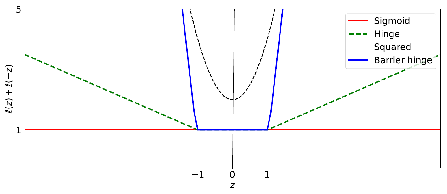
Figure 3: The plot of $\ell(z)+\ell(-z)$ of classification-calibrated losses. Only the sigmoid loss is symmetric. The hinge loss and barrier hinge loss satisfy the symmetric condition in $z\in[-1,1]$.

Definition 12.

A barrier hinge loss is defined as

$$\ell(z)=\mathrm{max}(-b(r+z)+r,\mathrm{max}(b(z-r),r-z))\text{,}$$

where $b>1$ and $r>0$.

Figure 2 shows a scaled barrier hinge loss with a specific parameter. Since a barrier hinge loss is convex, it is simple to verify that it is classification-calibrated since the derivative of the barrier hinge loss at zero is negative (Bartlett et al., 2006). Intuitively, barrier hinge losses are designed to give a very high penalty when $z$ is in the non-symmetric area. As a result, a prediction function which is learned from a barrier hinge loss has an incentive to give a prediction value inside the symmetric area. The parameter $r$ determines the width of the region that satisfies the symmetric property while the parameter $b$ determines the slope of the penalty when $z$ is in the non-symmetric area ($b$ is expected to be a large value). In the experiment section, we show that our barrier hinge loss benefits from the symmetric condition and more robust than other non-symmetric losses. For fairness, we fix $b=200$ and $r=50$ for all datasets in the experiment section. Hence, one can further tune the parameters $b$ and $r$ to achieve a more preferable performance.

It is important to note that if we restrict the output of a loss to be in a symmetric region, e.g., $g(\boldsymbol{x})\in[-1,1]$ and $r\geq 1$, using the barrier hinge loss, unhinged loss, or standard hinge loss, are equivalent. Thus, the barrier hinge loss can also be viewed as a soft-constrained version of the unhinged loss.

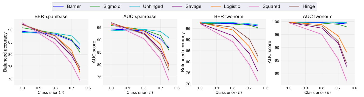
Figure 4: Mean balanced accuracy (1-BER) and AUC score using multilayer perceptrons (rescaled to 0-100) with varying noise rates $(\pi=1.0,\pi^{\prime}=0.0),(\pi=0.8,\pi^{\prime}=0.3),(\pi=0.7,\pi^{\prime}=0.4),(\pi=0.65,\pi^{\prime}=0.45)$. The experiments were conducted 20 times.

Table 2: Mean balanced accuracy (BAC=1-BER) and AUC score using multilayer perceptrons (rescaled to 0-100), where $\pi=0.65$ and $\pi^{\prime}=0.45$. Outperforming methods are highlighted in boldface using one-sided t-test with the significance level 5%. The experiments were conducted 20 times.

Dataset	Task	Barrier	Unhinged	Sigmoid	Logistic	Hinge	Squared	Savage
spambase	BAC	$82.3(0.8)$	84.1 (0.6)	$80.9(0.6)$	$72.6(0.7)$	$74.7(0.7)$	$69.5(0.7)$	$73.6(0.6)$
	AUC	$86.8(0.7)$	90.9 (0.4)	$86.0(0.4)$	$79.2(0.8)$	$77.7(0.7)$	$73.6(0.8)$	$80.1(0.8)$
waveform	BAC	86.1 (0.4)	87.1 (0.6)	$85.4(0.6)$	$75.8(0.7)$	$78.3(0.7)$	$69.2(0.6)$	$73.2(0.6)$
	AUC	92.2 (0.4)	91.7 (0.6)	90.9 (0.6)	$82.3(0.7)$	$79.8(0.9)$	$75.1(0.7)$	$80.1(0.6)$
twonorm	BAC	96.2 (0.3)	96.7 (0.2)	$95.4(0.4)$	$80.2(0.5)$	$82.8(0.9)$	$71.6(0.7)$	$75.9(0.6)$
	AUC	$99.1(0.1)$	99.6 (0.0)	$98.0(0.2)$	$88.3(0.5)$	$83.9(0.7)$	$77.3(0.7)$	$82.7(0.5)$
mushroom	BAC	93.4 (0.8)	$91.1(0.9)$	94.4 (0.7)	$81.3(0.5)$	$84.5(1.0)$	$72.2(0.6)$	$79.5(0.8)$
	AUC	98.4 (0.2)	$97.2(0.4)$	97.8 (0.3)	$89.0(0.5)$	$82.2(0.6)$	$77.8(0.6)$	$88.1(0.7)$

6 Experimental Results

In this section, we present experimental results of BER and AUC optimization from corrupted labels. We used the balanced accuracy (1-BER) to evaluate the performance of BER minimization and the AUC score for AUC maximization. We also rescaled the score to be from 0 to 100. Note that higher balanced accuracy and AUC score are better. Training data were corrupted manually by simply mixing positive and negative data according to the class prior of the corrupted positive and corrupted negative data, i.e., $\pi$ and $\pi^{\prime}$. We compare the following loss functions: the squared loss, logistic loss, exponential loss, hinge loss, savage loss, sigmoid loss, unhinged loss, and barrier loss. Note that the class prior information is not given to the classifier. Moreover, only the sigmoid loss and unhinged loss are symmetric while our proposed barrier loss is not symmetric everywhere but is designed to benefit from the symmetric condition. One might suspect that the improvement of the performance comes from the fact that these symmetric losses are bounded from above and therefore more robust against noise. To emphasize the importance of the symmetric property, we also compare the performance with the savage loss, a loss function which is bounded and has demonstrated its robustness against outliers in classification (Masnadi-Shirazi & Vasconcelos, 2009). We also found that the double hinge loss (du Plessis et al., 2015) performed similarly to the hinge loss and thus we omit the results.

We design the experiments to answer the following three questions. First, does the symmetric condition helps significantly in BER and AUC optimization from corrupted labels? Second, do we need a loss to be symmetric everywhere to benefit from the robustness of symmetric losses? Third, does the negative unboundedness of the unhinged loss degrade the practical performance?

6.1 Experiments on UCI and LIBSVM Datasets

In this experiment, we used the one hidden layer multilayer perceptron $d-500-1$ as a model. We used datasets from the UCI machine learning repository (Lichman et al., 2013) and LIBSVM (Chang & Lin, 2011). Training data consists of 500 corrupted positive data, 500 corrupted negative data, and balanced 500 clean test data. More details on the implementation, datasets, and full experimental results using more datasets can be found in Appendix. The objective functions of the neural networks were optimized using AMSGRAD (Reddi et al., 2018). The experiment code was implemented with Chainer (Tokui et al., 2015).

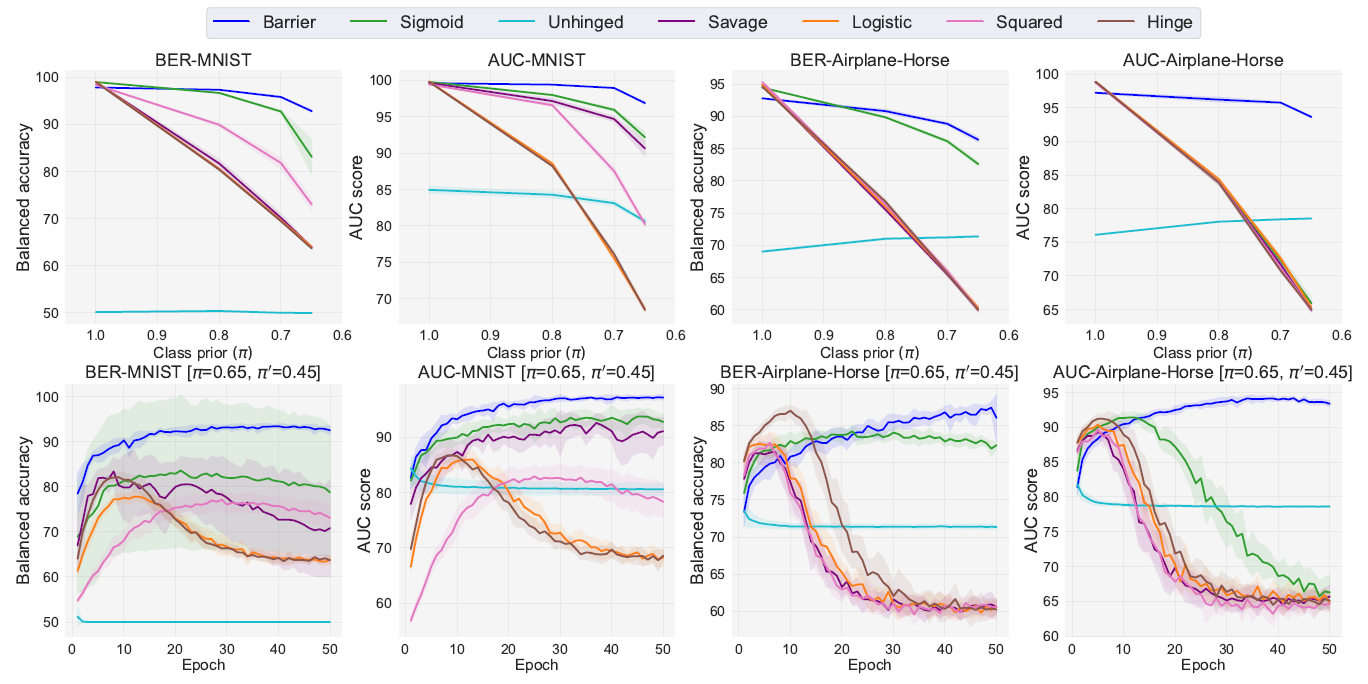
Figure 5: Mean balanced accuracy (1-BER) and AUC score using convolutional neural networks (rescaled to 0-100). (Top) the varying noise rates ranged from$(\pi=1.0,\pi^{\prime}=0.0),(\pi=0.8,\pi^{\prime}=0.3),(\pi=0.7,\pi^{\prime}=0.4),(\pi=0.65,\pi^{\prime}=0.45)$. (Bottom) the noise rate is $\pi=0.65$ and $\pi^{\prime}=0.45$. The experiments were conducted 10 times.

Figure 4 shows the performance of BER and AUC optimization with varying noise rates $(\pi=1.0,\pi^{\prime}=0.0),(\pi=0.8,\pi^{\prime}=0.3),(\pi=0.7,\pi^{\prime}=0.4),(\pi=0.65,\pi^{\prime}=0.45)$. Table 2 also shows the results where labels are highly corrupted ($\pi=0.65$ and $\pi^{\prime}=0.45$). Although the savage loss is a bounded loss, its performance is not desirable when the labels are corrupted. It can be observed that when the data is clean ($\pi=1.0$ and $\pi^{\prime}=0.0$), the performance of all losses are not significantly different. However, as the noise rate increases, the sigmoid loss, unhinged loss, and barrier loss significantly outperform other losses in this experiment. This suggests that only using a bounded loss is not sufficient to perform BER minimization from corrupted labels effectively. Therefore, the experimental results support our hypothesis that using symmetric losses can be preferable in the BER minimization problem from corrupted labels.

In this experiment, the unhinged loss performs well although it is negatively unbounded. This positive result of the unhinged loss agrees with van Rooyen et al. (2015a), where they used a linear-in-input model. However, our next experiment shows that the performance of the unhinged loss is less desirable when deeper neural networks are applied.

6.2 Experiments on MNIST and CIFAR-10

In this experiment, we used MNIST (LeCun, 1998) (Odd vs Even) and CIFAR-10 (Airplane vs Horse) (Krizhevsky & Hinton, 2009) as the datasets. We used the convolutional neural networks as the models for all losses. Full experimental results including the experiments on additional eight pairs of CIFAR10 and the implementation details can be found in Appendix. The objective functions were optimized using AMSGRAD (Reddi et al., 2018). The experiment code was implemented with PyTorch (Paszke et al., 2017).

Figure 5 (top) shows the performance on BER and AUC optimization with varying noise rates similarly to the previous experiment. It is observed that the unhinged loss failed miserably in BER minimization, although it outperformed other baselines when the labels are highly corrupted in CIFAR-10 (Airplane vs Horse). Our proposed barrier hinge loss is observed to be advantageous in this experiment.

Figure 5 (bottom) shows the performance on BER and AUC optimization from highly corrupted labels $(\pi=0.65,\pi^{\prime}=0.45)$ as the training epoch increases. The unhinged loss is observed to converge very quickly but its performance is marginal. The performance of the barrier hinge loss is preferable and does not degrade as the number of epoch increases. For the sigmoid loss, it is observed that the performance also degraded for the AUC maximization in CIFAR-10 as the epoch increases although it degraded slower than other losses that do not benefit from the symmetric condition.

In summary, our experimental results support that the symmetric condition significantly contributes to improving the performance on BER and AUC optimization from corrupted labels. Our barrier hinge loss, which is not symmetric everywhere, also demonstrated its robustness in this experiment. Finally, the unhinged loss is observed to perform poorly when complex models such as the convolutional neural networks are applied for which the potential reason can be the negative unboundedness of the unhinged loss.

7 Conclusion

We analyze a class of symmetric losses. We showed that the symmetric condition of a loss contributes to the robustness of the BER and AUC optimization from corrupted labels. Moreover, we proved the general theoretical results to provide a better understanding of symmetric losses. We also proposed a convex barrier hinge loss that is not symmetric everywhere but benefits greatly from the symmetric condition. The experimental results showed the advantage of using a symmetric loss for the BER and AUC optimization from corrupted labels and also illustrated the problem when a loss is negatively unbounded, such as the unhinged loss.

Appendix A Proofs

We provide the proofs in this section.

A.1 Proof of Theorem 1

Proof.

Recall that the AUC risk is:

$$R^{\ell}_{\mathrm{AUC}}(g)=\mathbb{E}_{\mathrm{P}}[\mathbb{E}_{\mathrm{N}}[\ell(f(\boldsymbol{x}_{\mathrm{P}},\boldsymbol{x}_{\mathrm{N}}))]]\text{.}$$

Corrupted AUC risk where $X_{\mathrm{CP}}$ is assigned to be positive and $X_{\mathrm{CN}}$ as negative:

$$R^{\ell}_{\mathrm{AUC}\text{-}\mathrm{Corr}}(g)=\mathbb{E}_{\mathrm{CP}}[\mathbb{E}_{\mathrm{CN}}[\ell(f(\boldsymbol{x}_{\mathrm{CP}},\boldsymbol{x}_{\mathrm{CN}}))]]\text{.}$$

where

$$R_{\mathrm{CP}}^{\ell}(g) =\pi\mathbb{E}_{\mathrm{P}}[\ell(g(\boldsymbol{x}))]+(1-\pi)\mathbb{E}_{\mathrm{N}}[\ell(g(\boldsymbol{x}))]\text{,}$$

$$R_{\mathrm{CN}}^{\ell}(g) =\pi^{\prime}\mathbb{E}_{\mathrm{P}}[\ell(-g(\boldsymbol{x}))]+(1-\pi^{\prime})\mathbb{E}_{\mathrm{N}}[\ell(-g(\boldsymbol{x}))]\text{.}$$

$R^{\ell}_{\mathrm{AUC}\text{-}\mathrm{Corr}}(g)$ can be rewritten as follows:

$$R^{\ell}_{\mathrm{AUC}\text{-}\mathrm{Corr}}(g)={} \pi^{\prime}\mathbb{E}_{\mathrm{CP}}[\mathbb{E}_{\mathrm{P}}[\ell(f(\boldsymbol{x}_{\mathrm{CP}},\boldsymbol{x}_{\mathrm{P}}))]]+(1-\pi^{\prime})\mathbb{E}_{\mathrm{CP}}[\mathbb{E}_{\mathrm{N}}[\ell(f(\boldsymbol{x}_{\mathrm{CP}},\boldsymbol{x}_{\mathrm{N}}))]]]$$

$$\begin{split}={}&\pi\pi^{\prime}\mathbb{E}_{\mathrm{P^{\prime}}}[\mathbb{E}_{\mathrm{P}}[\ell(f(\boldsymbol{x}_{\mathrm{P^{\prime}}},\boldsymbol{x}_{\mathrm{P}}))]]+(1-\pi)\pi^{\prime}\mathbb{E}_{\mathrm{N}}[\mathbb{E}_{\mathrm{P}}[\ell(f(\boldsymbol{x}_{\mathrm{N}},\boldsymbol{x}_{\mathrm{P}}))]]\\ &+\pi(1-\pi^{\prime})\mathbb{E}_{\mathrm{P}}[\mathbb{E}_{\mathrm{N}}[\ell(f(\boldsymbol{x}_{\mathrm{P}},\boldsymbol{x}_{\mathrm{N}}))]]\\ &+(1-\pi)(1-\pi^{\prime})\mathbb{E}_{\mathrm{N^{\prime}}}[\mathbb{E}_{\mathrm{N}}[\ell(f(\boldsymbol{x}_{\mathrm{N^{\prime}}},\boldsymbol{x}_{\mathrm{N}}))]]\text{.}\end{split}$$

Let

$$A =\mathbb{E}_{\mathrm{P^{\prime}}}[\mathbb{E}_{\mathrm{P}}[\ell(f(\boldsymbol{x}_{\mathrm{P^{\prime}}},\boldsymbol{x}_{\mathrm{P}}))]]\,\text{,}$$

$$B =\mathbb{E}_{\mathrm{N}}[\mathbb{E}_{\mathrm{P}}[\ell(f(\boldsymbol{x}_{\mathrm{N}},\boldsymbol{x}_{\mathrm{P}}))]]\text{,}$$

$$C =\mathbb{E}_{\mathrm{P}}[\mathbb{E}_{\mathrm{N}}[\ell(f(\boldsymbol{x}_{\mathrm{P}},\boldsymbol{x}_{\mathrm{N}}))]]=R^{\ell}_{\mathrm{AUC}}(g)\text{,}$$

$$D =\mathbb{E}_{\mathrm{N^{\prime}}}[\mathbb{E}_{\mathrm{N}}[\ell(f(\boldsymbol{x}_{\mathrm{N^{\prime}}},\boldsymbol{x}_{\mathrm{N}}))]]\text{,}$$

$$\gamma^{\ell} =\mathbb{E}_{\mathrm{P}}[\mathbb{E}_{\mathrm{N}}[\ell(f(\boldsymbol{x}_{\mathrm{P}},\boldsymbol{x}_{\mathrm{N}}))+\ell(f(\boldsymbol{x}_{\mathrm{N}},\boldsymbol{x}_{\mathrm{P}}))]]=B+C\text{,}$$

$$\gamma^{\ell}(\boldsymbol{x},\boldsymbol{x}^{\prime}) =\ell(f(\boldsymbol{x},\boldsymbol{x}^{\prime}))+\ell(f(\boldsymbol{x}^{\prime},\boldsymbol{x}))\text{.}$$

First, we show that $A=\mathbb{E}_{\mathrm{P^{\prime}}}[\mathbb{E}_{\mathrm{P}}[\ell(f(\boldsymbol{x}_{\mathrm{P^{\prime}}},\boldsymbol{x}_{\mathrm{P}}))]]=\mathbb{E}_{\mathrm{P^{\prime}}}[\mathbb{E}_{\mathrm{P}}[\frac{\gamma^{\ell}(\boldsymbol{x}_{\mathrm{P^{\prime}}},\boldsymbol{x}_{\mathrm{P}})}{2}]]$:

$$\mathbb{E}_{\mathrm{P^{\prime}}}[\mathbb{E}_{\mathrm{P}}[\ell(f(\boldsymbol{x}_{\mathrm{P^{\prime}}},\boldsymbol{x}_{\mathrm{P}}))]] =\mathbb{E}_{\mathrm{P^{\prime}}}[\mathbb{E}_{\mathrm{P}}[\mathbbm{1}_{\boldsymbol{x}_{\mathrm{P^{\prime}}}=\boldsymbol{x}_{\mathrm{P}}}\ell(0)+\mathbbm{1}_{\boldsymbol{x}_{\mathrm{P^{\prime}}}\neq\boldsymbol{x}_{\mathrm{P}}}\ell(f(\boldsymbol{x}_{\mathrm{P^{\prime}}},\boldsymbol{x}_{\mathrm{P}}))]]$$

$$=\mathbb{E}_{\mathrm{P^{\prime}}}[\mathbb{E}_{\mathrm{P}}[\mathbbm{1}_{\boldsymbol{x}_{\mathrm{P^{\prime}}}=\boldsymbol{x}_{\mathrm{P}}}\ell(0)]]+\mathbb{E}_{\mathrm{P^{\prime}}}[\mathbb{E}_{\mathrm{P}}[\mathbbm{1}_{\boldsymbol{x}_{\mathrm{P^{\prime}}}\neq\boldsymbol{x}_{\mathrm{P}}}\ell(f(\boldsymbol{x}_{\mathrm{P^{\prime}}},\boldsymbol{x}_{\mathrm{P}}))]]$$

$$=0+\mathbb{E}_{\mathrm{P^{\prime}}}[\mathbb{E}_{\mathrm{P}}[1\times\ell(f(\boldsymbol{x}_{\mathrm{P^{\prime}}},\boldsymbol{x}_{\mathrm{P}}))]$$

$$=\mathbb{E}_{\mathrm{P^{\prime}}}[\mathbb{E}_{\mathrm{P}}[\frac{\ell(f(\boldsymbol{x}_{\mathrm{P^{\prime}}},\boldsymbol{x}_{\mathrm{P}}))+\ell(f(\boldsymbol{x}_{\mathrm{P}},\boldsymbol{x}_{\mathrm{P^{\prime}}}))}{2}]]$$

$$=\mathbb{E}_{\mathrm{P^{\prime}}}[\mathbb{E}_{\mathrm{P}}[\frac{\gamma^{\ell}(\boldsymbol{x}_{\mathrm{P^{\prime}}},\boldsymbol{x}_{\mathrm{P}})}{2}]]\text{.}$$

D can also be rewritten in a same manner so it is omitted for brevity.

$$D=\mathbb{E}_{\mathrm{N^{\prime}}}[\mathbb{E}_{\mathrm{N}}[\ell(f(\boldsymbol{x}_{\mathrm{N^{\prime}}},\boldsymbol{x}_{\mathrm{N}}))]]=\mathbb{E}_{\mathrm{N^{\prime}}}[\mathbb{E}_{\mathrm{N}}[\frac{\gamma^{\ell}(\boldsymbol{x}_{\mathrm{N^{\prime}}},\boldsymbol{x}_{\mathrm{N}})}{2}]]\text{.}$$

Then, we get the following result:

$$R^{\ell}_{\mathrm{AUC}\text{-}\mathrm{Corr}}(g)={} \pi\pi^{\prime}A+(1-\pi)\pi^{\prime}B+\pi(1-\pi^{\prime})C+(1-\pi)(1-\pi^{\prime})D$$

$$={} \pi\pi^{\prime}A+(1-\pi)\pi^{\prime}(\gamma^{\ell}-C)+\pi(1-\pi^{\prime})C+(1-\pi)(1-\pi^{\prime})D$$

$$={} \pi\pi^{\prime}A+(\pi^{\prime}-\pi\pi^{\prime})\gamma^{\ell}+(\pi-\pi^{\prime})C+(1-\pi)(1-\pi^{\prime})D$$

$$\begin{split}={}&(\pi-\pi^{\prime})R^{\ell}_{\mathrm{AUC}}(g)+(1-\pi)\pi^{\prime}\mathbb{E}_{\mathrm{P}}[\mathbb{E}_{\mathrm{N}}[\gamma^{\ell}(\boldsymbol{x}_{\mathrm{P}},\boldsymbol{x}_{\mathrm{N}})]]\\ &+\pi\pi^{\prime}\mathbb{E}_{\mathrm{P^{\prime}}}[\mathbb{E}_{\mathrm{P}}[\frac{\gamma^{\ell}(\boldsymbol{x}_{\mathrm{P^{\prime}}},\boldsymbol{x}_{\mathrm{P}})}{2}]]+(1-\pi)(1-\pi^{\prime})\mathbb{E}_{\mathrm{N^{\prime}}}[\mathbb{E}_{\mathrm{N}}[\frac{\gamma^{\ell}(\boldsymbol{x}_{\mathrm{N^{\prime}}},\boldsymbol{x}_{\mathrm{N}})}{2}]]\\ \end{split}$$

$$\begin{split}={}&(\pi-\pi^{\prime})R^{\ell}_{\mathrm{AUC}}(g)+(\pi^{\prime}-\pi\pi^{\prime})\mathbb{E}_{\mathrm{P}}[\mathbb{E}_{\mathrm{N}}[\gamma^{\ell}(\boldsymbol{x}_{\mathrm{P}},\boldsymbol{x}_{\mathrm{N}})]]\\ &+\frac{\pi\pi^{\prime}}{2}\mathbb{E}_{\mathrm{P^{\prime}}}[\mathbb{E}_{\mathrm{P}}[\gamma^{\ell}(\boldsymbol{x}_{\mathrm{P^{\prime}}},\boldsymbol{x}_{\mathrm{P}})]]+\frac{(1-\pi)(1-\pi^{\prime})}{2}\mathbb{E}_{\mathrm{N^{\prime}}}[\mathbb{E}_{\mathrm{N}}[\gamma^{\ell}(\boldsymbol{x}_{\mathrm{N^{\prime}}},\boldsymbol{x}_{\mathrm{N}})]]\text{.}\\ \end{split}$$

Therefore, minimizing $R^{\ell}_{\mathrm{AUC}\text{-}\mathrm{Corr}}(g)$ does not imply minimizing $R^{\ell}_{\mathrm{AUC}}(g)$ unless $\ell(f(\boldsymbol{x},\boldsymbol{x}^{\prime}))+\ell(f(\boldsymbol{x}^{\prime},\boldsymbol{x}))$ is a constant. ∎

A.2 Proof of Theorem 3

Let $\gamma^{\ell}(\boldsymbol{x})=\ell(g(\boldsymbol{x}))+\ell(-g(\boldsymbol{x}))$, $R^{\ell}_{\mathrm{BER}\text{-}\mathrm{Corr}}(g)$ can be expressed as

$$R^{\ell}_{\mathrm{BER}\text{-}\mathrm{Corr}}(g)={} (\pi-\pi^{\prime}){R^{\ell}_{\mathrm{BER}}(g)}+\frac{\pi^{\prime}\mathbb{E}_{\mathrm{P}}[\gamma^{\ell}(\boldsymbol{x})]+(1-\pi)\mathbb{E}_{\mathrm{N}}[\gamma^{\ell}(\boldsymbol{x})]}{2}$$

Proof.

Recall that the balanced risk is:

$$R^{\ell}_{\mathrm{BER}}(g) =\frac{1}{2}\big{[}\mathbb{E}_{\mathrm{P}}[\ell(g(\boldsymbol{x}))\big{]}+\mathbb{E}_{\mathrm{N}}\big{[}\ell(-g(\boldsymbol{x}))]\big{]}\text{.}$$

Balanced corrupted risk where $X_{\mathrm{CP}}$ is assigned to be positive and $X_{\mathrm{CN}}$ as negative:

$$R^{\ell}_{\mathrm{BER}\text{-}\mathrm{Corr}}(g)=\frac{1}{2}\big{[}R_{\mathrm{CP}}^{\ell}(g)+R_{\mathrm{CN}}^{\ell}(g)\big{]}\text{,}$$

where

$$R_{\mathrm{CP}}^{\ell}(g) =\pi\mathbb{E}_{\mathrm{P}}[\ell(g(\boldsymbol{x}))]+(1-\pi)\mathbb{E}_{\mathrm{N}}[\ell(g(\boldsymbol{x}))]\text{,}$$

$$R_{\mathrm{CN}}^{\ell}(g) =\pi^{\prime}\mathbb{E}_{\mathrm{P}}[\ell(-g(\boldsymbol{x}))]+(1-\pi^{\prime})\mathbb{E}_{\mathrm{N}}[\ell(-g(\boldsymbol{x}))]\text{.}$$

$R^{\ell}_{\mathrm{BER}\text{-}\mathrm{Corr}}(g)$ can be rewritten as follows:

$$\begin{split}2R^{\ell}_{\mathrm{BER}\text{-}\mathrm{Corr}}(g)={}&\pi\mathbb{E}_{\mathrm{P}}[\ell(g(\boldsymbol{x}))]+(1-\pi)\mathbb{E}_{\mathrm{N}}[\ell(g(\boldsymbol{x}))]\\ &+\pi^{\prime}\mathbb{E}_{\mathrm{P}}[\ell(-g(\boldsymbol{x}))]+(1-\pi^{\prime})\mathbb{E}_{\mathrm{N}}[\ell(-g(\boldsymbol{x}))]\end{split}$$

$$\begin{split}={}&\pi\mathbb{E}_{\mathrm{P}}[\ell(g(\boldsymbol{x}))]+(1-\pi)\mathbb{E}_{\mathrm{N}}[\gamma^{\ell}(\boldsymbol{x})-\ell(-g(\boldsymbol{x}))]\\ &+\pi^{\prime}\mathbb{E}_{\mathrm{P}}[\gamma^{\ell}(\boldsymbol{x})-\ell(g(\boldsymbol{x}))]+(1-\pi^{\prime})\mathbb{E}_{\mathrm{N}}[\ell(-g(\boldsymbol{x}))]\end{split}$$

$$\begin{split}={}&\pi\mathbb{E}_{\mathrm{P}}[\ell(g(\boldsymbol{x}))]+(1-\pi)\mathbb{E}_{\mathrm{N}}[\gamma^{\ell}(\boldsymbol{x})]-(1-\pi)\mathbb{E}_{\mathrm{N}}[\ell(-g(\boldsymbol{x}))]\\ &+\pi^{\prime}\mathbb{E}_{\mathrm{P}}[\gamma^{\ell}(\boldsymbol{x})]-\pi^{\prime}\mathbb{E}_{\mathrm{P}}[\ell(g(\boldsymbol{x}))]+(1-\pi^{\prime})\mathbb{E}_{\mathrm{N}}[\ell(-g(\boldsymbol{x}))]\end{split}$$

$$\begin{split}={}&\pi\mathbb{E}_{\mathrm{P}}[\ell(g(\boldsymbol{x}))]-\pi^{\prime}\mathbb{E}_{\mathrm{N}}[\ell(-g(\boldsymbol{x}))]+\pi\mathbb{E}_{\mathrm{N}}[\ell(-g(\boldsymbol{x}))]\\ &-\pi^{\prime}\mathbb{E}_{\mathrm{P}}[\ell(g(\boldsymbol{x}))]+(1-\pi)\mathbb{E}_{\mathrm{N}}[\gamma^{\ell}(\boldsymbol{x})]+\pi^{\prime}\mathbb{E}_{\mathrm{P}}[\gamma^{\ell}(\boldsymbol{x})]\end{split}$$

$$={} (\pi-\pi^{\prime})[\mathbb{E}_{\mathrm{P}}[\ell(g(\boldsymbol{x}))]+\mathbb{E}_{\mathrm{N}}[\ell(-g(\boldsymbol{x}))]]+\pi^{\prime}\mathbb{E}_{\mathrm{P}}[\gamma^{\ell}(\boldsymbol{x})]+(1-\pi)\mathbb{E}_{\mathrm{N}}[\gamma^{\ell}(\boldsymbol{x})]$$

$$={} 2(\pi-\pi^{\prime})R^{\ell}_{\mathrm{BER}}(g)+\pi^{\prime}\mathbb{E}_{\mathrm{P}}[\gamma^{\ell}(\boldsymbol{x})]+(1-\pi)\mathbb{E}_{\mathrm{N}}[\gamma^{\ell}(\boldsymbol{x})]$$

$$R^{\ell}_{\mathrm{BER}\text{-}\mathrm{Corr}}(g)={} (\pi-\pi^{\prime}){R^{\ell}_{\mathrm{BER}}(g)}+\frac{\pi^{\prime}\mathbb{E}_{\mathrm{P}}[\gamma^{\ell}(\boldsymbol{x})]+(1-\pi)\mathbb{E}_{\mathrm{N}}[\gamma^{\ell}(\boldsymbol{x})]}{2}\text{.}$$

∎

A.3 Conditional risk for binary classification

By making use of the symmetric property, i.e., $\ell(z)+\ell(-z)=K$, a pointwise conditional risk can be rewritten such that there is only one term depending on $\alpha$ as follows for a fixed $\boldsymbol{x}$:

$$C^{\ell}_{\eta}(\alpha) =\eta\ell(\alpha)+(1-\eta)\ell(-\alpha)$$

$$=\eta\ell(\alpha)+(1-\eta)(K-\ell(\alpha))$$

$$=(1-\eta)K+(2\eta-1)\ell(\alpha)\text{,}$$

where $\eta=p(y=1|\boldsymbol{x})$. It can be observed that $\ell(-z)$ can be expressed by $K-\ell(z)$. The symmetric property makes analysis simpler because $\ell(-z)$ can be rewritten as $\ell(z)$and the following general properties can be obtained by only rely on the symmetric property.

A.4 Proof of Theorem 5

Proof.

Let $H(\eta)=\inf\limits_{\alpha\in\mathbb{R}}C^{\ell}_{\eta}(\alpha)$ and $H^{-}(\eta)=\inf\limits_{\alpha:\alpha(2\eta-1)\leq 0}C^{\ell}_{\eta}(\alpha)$ .

First, consider the $\psi$-transform from the definition 2 of Bartlett et al. (2006). Consider $\ell\colon\mathbb{R}\to[0,\infty)$, function $\psi:[0,1]\to[0,\infty)$ by $\psi=\tilde{\psi}^{**}$, where

$$\tilde{\psi}(\theta)=H^{-}\bigg{(}\frac{1+\theta}{2}\bigg{)}-H\bigg{(}\frac{1+\theta}{2}\bigg{)},$$

$g^{**}\colon[0,1]\to\mathbb{R}$ is the Fenchel-Legendre biconjugate of $g:[0,1]\to\mathbb{R}$ characterized by

$$\mathrm{epi}\,g^{**}=\overline{co}\,\mathrm{epi}\,g.$$

It is known that $\psi=\tilde{\psi}$ if and only if $\tilde{\psi}$ is convex. For more details, please refer to Bartlett et al. (2006).

Next, we use the following statements in Lemma 5 from Bartlett et al. (2006) which can be interpreted that, $\ell$ is classification-calibrated if and only if $\psi(\theta)>0$ for all $\theta\in(0,1]$. Based on this statement, we prove the sufficient and necessary condition for symmetric losses to be classification-calibrated by showing that $\psi(\theta)>0$ for all $\theta\in(0,1]$ if and only if $\inf\limits_{\alpha>0}\ell(\alpha)<\inf\limits_{\alpha\leq 0}\ell(\alpha)$.

Using the conditional risk of symmetric losses in the previous section, $H$ and $H^{-}$ can be written as

$$H(\eta) =\inf\limits_{\alpha\in\mathbb{R}}C^{\ell}_{\eta}(\alpha)$$

$$=(1-\eta)K+\inf\limits_{\alpha\in\mathbb{R}}(2\eta-1)\ell(\alpha)\text{,}$$

$$H^{-}(\eta) =\inf\limits_{\alpha:\alpha(2\eta-1)\leq 0}C^{\ell}_{\eta}(\alpha)$$

$$=(1-\eta)K+\inf\limits_{\alpha:\alpha(2\eta-1)\leq 0}(2\eta-1)\ell(\alpha)\text{.}$$

Let $\tilde{\psi}(\theta)=H^{-}(\frac{1+\theta}{2})-H(\frac{1+\theta}{2})$ where $\theta\in(0,1]$,

$$\tilde{\psi}(\theta) =H^{-}(\frac{1+\theta}{2})-H(\frac{1+\theta}{2})$$

$$=\inf\limits_{\alpha:\alpha\theta\leq 0}\theta\ell(\alpha)-\inf\limits_{\alpha\in\mathbb{R}}\theta\ell(\alpha)$$

$$=\theta[\inf\limits_{\alpha\leq 0}\ell(\alpha)-\inf\limits_{\alpha\in\mathbb{R}}\ell(\alpha)]\text{.}$$

Let $\mathrm{C}=\inf\limits_{\alpha\leq 0}\ell(\alpha)-\inf\limits_{\alpha\in\mathbb{R}}\ell(\alpha)$ is a constant depends on the function.

$$\tilde{\psi}(\theta) =C\theta\text{.}$$

Here, $\tilde{\psi}(\theta)$ is linear and therefore convex. As a result, $\psi=\tilde{\psi}$. Based on Lemma 5 of Bartlett et al. (2006). $\ell$ is classification-callibrated if and only if $\psi(\theta)>0$ for all $\theta\in(0,1].$ In this case, $\theta$ is positive therefore, any symmetric loss function is classification-calibrated if and only if $C>0$.

$$\inf\limits_{\alpha\leq 0}\ell(\alpha)-\inf\limits_{\alpha\in\mathbb{R}}\ell(\alpha) >0$$

$$\inf\limits_{\alpha\in\mathbb{R}}\ell(\alpha) <\inf\limits_{\alpha\leq 0}\ell(\alpha)$$

$$\inf\limits_{\alpha>0}\ell(\alpha) <\inf\limits_{\alpha\leq 0}\ell(\alpha)\text{.}$$

Therefore, a symmetric loss $\ell$ is classification-calibrated if and only if $\inf\limits_{\alpha>0}\ell(\alpha)<\inf\limits_{\alpha\leq 0}\ell(\alpha)$. ∎

A.5 Proof of Theorem 7

Proof.

Once $\psi(\theta)=[\inf\limits_{\alpha\leq 0}\ell(\alpha)-\inf\limits_{\alpha>0}\ell(\alpha)]\theta$ is obtained in the previous proof of classification-calibration for a symmetric loss. It is straightforward to obtain an excess risk bound based on Bartlett et al. (2006):

$$\psi(R^{\ell_{0\text{-}1}}(g)-R^{\ell_{0\text{-}1}*}) \leq R^{\ell}(g)-R^{\ell*}$$

$$[\inf\limits_{\alpha\leq 0}\ell(\alpha)-\inf\limits_{\alpha>0}\ell(\alpha)](R^{\ell_{0\text{-}1}}(g)-R^{\ell_{0\text{-}1}*}) \leq R^{\ell}(g)-R^{\ell*}$$

$$R^{\ell_{0\text{-}1}}(g)-R^{\ell_{0\text{-}1}*} \leq\frac{R^{\ell}(g)-R^{\ell*}}{\inf\limits_{\alpha\leq 0}\ell(\alpha)-\inf\limits_{\alpha>0}\ell(\alpha)}\text{,}$$

where $R^{\ell*}=\inf\limits_{g}R^{\ell}(g)$ and $R^{\ell_{0\text{-}1}*}=\inf\limits_{g}R^{\ell_{0\text{-}1}}(g)$. ∎

A.6 Proof of Theorem 8

Proof.

Consider a conditional risk minimizer of a symmetric loss $\ell$

$$f_{\ell}^{*}(\boldsymbol{x}) =\operatorname*{arg\,min}\limits_{\alpha\in\mathbb{R}}C^{\ell}_{\eta(\boldsymbol{x})}(\alpha)$$

$$=\operatorname*{arg\,min}\limits_{\alpha\in\mathbb{R}}(1-\eta(\boldsymbol{x}))K+(2\eta(\boldsymbol{x})-1)\ell(\alpha)\text{.}$$

The constants can be ignored as it does not depend on $\alpha$. Let us consider two cases of $\eta>\frac{1}{2}$ and $\eta<\frac{1}{2}$:

Case 1: $\eta>\frac{1}{2}$

$$f_{\ell}^{*}(\boldsymbol{x}) =(1-\eta(\boldsymbol{x}))K+\operatorname*{arg\,min}\limits_{\alpha\in\mathbb{R}}(2\eta(\boldsymbol{x})-1)\ell(\alpha)$$

$$=\operatorname*{arg\,min}\limits_{\alpha\in\mathbb{R}}\ell(\alpha)\text{.}$$

Case 2: $\eta<\frac{1}{2}$

$$f_{\ell}^{*}(\boldsymbol{x}) =(1-\eta(\boldsymbol{x}))K+\operatorname*{arg\,min}\limits_{\alpha\in\mathbb{R}}(2\eta(\boldsymbol{x})-1)\ell(\alpha)$$

$$=\operatorname*{arg\,max}\limits_{\alpha\in\mathbb{R}}\ell(\alpha)\text{.}$$

Suppose there are many $\alpha$ to satisfy the conditions. Due to the symmetric condition, We can express the following relations.

$$\operatorname*{arg\,min}\limits_{\alpha\in\mathbb{R}}\ell(\alpha)=-\operatorname*{arg\,max}\limits_{\alpha\in\mathbb{R}}\ell(\alpha)\text{,}$$

where $-\operatorname*{arg\,max}\limits_{\alpha\in\mathbb{R}}\ell(\alpha)$ means a set such that each element in the set $\operatorname*{arg\,max}\limits_{\alpha\in\mathbb{R}}\ell(\alpha)$ is multiplied by $-1$. As a result, $f_{\ell}^{*}(\boldsymbol{x})$ can be simply written as follows:

$$f_{\ell}^{*}(\boldsymbol{x})=\mathrm{M\,sign}(\eta(\boldsymbol{x})-\frac{1}{2})\text{,}$$

where M $\in\operatorname*{arg\,min}\limits_{\alpha\in\mathbb{R}}\ell(\alpha)$. This result shows that the conditional risk minimizer of a symmetric loss can be expressed as the bayes classifier scaled by a constant. In the case of functions such that it is classification-calibrated and argmin cannot be obtained, $M\to\infty$. ∎

A.7 Introduction of AUC-consistency

In AUC maximization, we want to find the function $g$ that minimizes the following risk:

$$R^{\ell_{0\text{-}1}}_{\mathrm{AUC}}(g)=\mathbb{E}_{\mathrm{P}}[\mathbb{E}_{\mathrm{N}}[\ell_{0\text{-}1}(g(\boldsymbol{x}_{\mathrm{P}})-g(\boldsymbol{x}_{\mathrm{N}}))]]\text{.}$$

Gao & Zhou (2015) showed that the Bayes optimal functions can be expressed as follows:

$$\mathcal{B} =\{g:R^{\ell_{0\text{-}1}}_{\mathrm{AUC}}(g)=R^{\ell_{0\text{-}1}*}_{\mathrm{AUC}}(g)\}$$

$$=\{g:(g(\boldsymbol{x})-g(\boldsymbol{x}^{\prime}))(\eta(\boldsymbol{x})-\eta(\boldsymbol{x}^{\prime}))>0\,\mathrm{if}\,\eta(\boldsymbol{x})\neq\eta(\boldsymbol{x}^{\prime})\}$$

Unlike classification-calibration, the Bayes optimal functions for AUC maximization depend on the pairwise class probability, i.e., the class probabilities for two data points are compared. The optimal function $g$ is a function such that the sign of $g(\boldsymbol{x})-g(\boldsymbol{x}^{\prime})$ matches the sign of $\eta(\boldsymbol{x})-\eta(\boldsymbol{x}^{\prime})$. Therefore, one solution of $g$ is the class probability itself. Because when $g(\boldsymbol{x})=\eta(\boldsymbol{x})$ for all $\boldsymbol{x}$, then $g(\boldsymbol{x})-g(\boldsymbol{x}^{\prime})=\eta(\boldsymbol{x})-\eta(\boldsymbol{x}^{\prime})$ which is exactly the same value as the function we want to match the sign with. As a result, it is arguable that the bipartite ranking problem based on the AUC score is easier than the class conditional probability estimation problem in the sense that the problem is solved if we have an access to $\eta(\boldsymbol{x})$. However, we only need to find a function $g$ such that $\mathrm{sign}(g(\boldsymbol{x})-g(\boldsymbol{x}^{\prime}))=\mathrm{sign}(\eta(\boldsymbol{x})-\eta(\boldsymbol{x}^{\prime}))$. AUC-consistency property can be treated as the minimum requirement of a loss function to be suitable for bipartite ranking (Gao & Zhou, 2015).

A.8 Proof of Lemma 9

A proof is based on a necessary of the notion of calibration in Gao & Zhou (2015), which we call AUC-calibration to avoid confusion in this paper. According to Gao & Zhou (2015), AUC-calibration is a necessary condition for AUC-consistency. Here, we prove that a symmetric loss is AUC-calibrated if and only if a symmetric loss is classification-calibrated.

Proof.

For a symmetric loss $\ell$, we can rewrite a pairwise conditional risk term in the infimum as follows:

$$\eta(1-\eta^{\prime})\ell(\alpha)+\eta^{\prime}(1-\eta)\ell(-\alpha) =\eta(1-\eta^{\prime})\ell(\alpha)+\eta^{\prime}(1-\eta)(K-\ell(\alpha))$$

$$=\eta(1-\eta^{\prime})\ell(\alpha)+\eta^{\prime}K(1-\eta)-\eta^{\prime}\ell(\alpha)+\eta\eta^{\prime}\ell(\alpha)$$

$$=(\eta-\eta^{\prime})\ell(\alpha)+\eta^{\prime}K(1-\eta)\text{.}$$

$$H^{-}(\eta,\eta^{\prime}) >H(\eta,\eta^{\prime})$$

$$H^{-}(\eta,\eta^{\prime})-H(\eta,\eta^{\prime}) >0$$

$$\frac{1}{2\pi(1-\pi)}[\inf\limits_{\alpha:\alpha(\eta-\eta^{\prime})\leq 0}(\eta-\eta^{\prime})\ell(\alpha)-\inf\limits_{\alpha\in\mathbb{R}}(\eta-\eta^{\prime})\ell(\alpha)] >0$$

$$\inf\limits_{\alpha:\alpha(\eta-\eta^{\prime})\leq 0}(\eta-\eta^{\prime})\ell(\alpha)-\inf\limits_{\alpha\in\mathbb{R}}(\eta-\eta^{\prime})\ell(\alpha) >0$$

Case 1: $\eta-\eta^{\prime}>0$

$$(\eta-\eta^{\prime})[\inf\limits_{\alpha:\alpha(\eta-\eta^{\prime})\leq 0}\ell(\alpha)-\inf\limits_{\alpha\in\mathbb{R}}\ell(\alpha)] >0$$

$$\inf\limits_{\alpha:\alpha\leq 0}\ell(\alpha)-\inf\limits_{\alpha\in\mathbb{R}}\ell(\alpha)>0\text{.}$$

Case 2: $\eta-\eta^{\prime}<0$

$$(\eta-\eta^{\prime})[\sup\limits_{\alpha:\alpha(\eta-\eta^{\prime})\leq 0}\ell(\alpha)-\sup\limits_{\alpha\in\mathbb{R}}\ell(\alpha)]>0$$

$$\sup\limits_{\alpha:\alpha(\eta-\eta^{\prime})\leq 0}\ell(\alpha)-\sup\limits_{\alpha\in\mathbb{R}}\ell(\alpha)<0$$

$$\sup\limits_{\alpha:\alpha\geq 0}\ell(\alpha)-\sup\limits_{\alpha\in\mathbb{R}}\ell(\alpha)<0\text{.}$$

The two inequalities are equivalent which proved in Section 4.9.6. Therefore, a symmetric loss must satisfy $\inf\limits_{\alpha>0}\ell(\alpha)<\inf\limits_{\alpha\leq 0}\ell(\alpha)$ to be AUC-calibrated. This is equivalent to classification-calibration condition for a symmetric loss. Next, it is known that AUC-calibration is a necessary condition for AUC-consistent (Gao & Zhou, 2015), therefore, a symmetric loss that is not classification-calibrated must not satisfy this condition, and thus not AUC-consistent.

This elucidates that classification-calibration is a necessary condition for a symmetric loss to be AUC-consistent. ∎

A.9 Proof of Proposition 10

Proof.

Consider a pairwise conditional risk:

$$\eta(1-\eta^{\prime})\ell(\alpha)+\eta^{\prime}(1-\eta)\ell(-\alpha) =\eta(1-\eta^{\prime})\ell(\alpha)+\eta^{\prime}(1-\eta)(K-\ell(\alpha))$$

$$=\eta(1-\eta^{\prime})\ell(\alpha)+\eta^{\prime}K(1-\eta)-\eta^{\prime}\ell(\alpha)+\eta\eta^{\prime}\ell(\alpha)$$

$$=(\eta-\eta^{\prime})\ell(\alpha)+\eta^{\prime}K(1-\eta)\text{.}$$ (3)

Then, let us consider a symmetric loss $\ell_{\mathrm{EX}}$ such that $\ell_{\mathrm{EX}}(1)=~{}0$, $\ell_{\mathrm{EX}}(-1)=1,$ and $0.5$ otherwise. It is straightforward to see that it is a symmetric loss where $\ell_{\mathrm{EX}}(z)+\ell_{\mathrm{EX}}(-z)=1$. We are going to show that this loss is classification-calibrated but AUC-consistent. Moreover, we can see that $\inf\limits_{\alpha>0}\ell_{\mathrm{EX}}(\alpha)<\inf\limits_{\alpha\leq 0}\ell_{\mathrm{EX}}(\alpha)$. Therefore, $\ell_{\mathrm{EX}}$ is classification-calibrated based on the previous theorem on a necessary and sufficient condition of a symmetric loss to be classification-calibrated.

Next, let us consider a uniform discrete distribution $D_{\mathrm{U}}$ that contains 3 possible supports $\{\boldsymbol{x}_{1},\boldsymbol{x}_{2},\boldsymbol{x}_{3}\}$. Moreover, let $\eta(\boldsymbol{x}_{1})=1$, $\eta(\boldsymbol{x}_{2})=0.5$, $\eta(\boldsymbol{x}_{3})=0$.

Here, we prove Proposition 10 by a counterexample that the minimizer of the AUC risk with respect to $\ell_{\mathrm{EX}}$ resulted in a function that behaves differently the Bayes-optimal solution of AUC maximization of a function that has a strictly monotonic relationship with the class probability $\eta(\boldsymbol{x})$ (Menon & Williamson, 2016), and therefore AUC-inconsistent.

Consider the following pairwise risk:

$$R^{\mathrm{pair}}_{\ell_{\mathrm{EX}}}(g) =\frac{1}{2\pi(1-\pi)}\mathop{\mathbb{E}}\limits_{\boldsymbol{x},\boldsymbol{x}^{\prime}\sim D^{2}_{X}}[\eta(\boldsymbol{x})(1-\eta(\boldsymbol{x}^{\prime}))\ell_{\mathrm{EX}}(g(\boldsymbol{x})-g(\boldsymbol{x}^{\prime}))$$

$$\quad+\eta(\boldsymbol{x}^{\prime})(1-\eta(\boldsymbol{x})\ell_{\mathrm{EX}}(g(\boldsymbol{x}^{\prime})-g(\boldsymbol{x}))]$$

$$=\frac{1}{2\pi(1-\pi)}\mathop{\mathbb{E}}\limits_{\boldsymbol{x},\boldsymbol{x}^{\prime}\sim D^{2}_{X}}[(\eta(\boldsymbol{x})-\eta(\boldsymbol{x}^{\prime}))\ell_{\mathrm{EX}}(g(\boldsymbol{x})-g(\boldsymbol{x}^{\prime}))+\eta^{\prime}K(1-\eta)]$$

Since we are only interested in the minimizer of the risk, let us ignore the constant term and rewrite the risk pair as follows:

$$R^{\mathrm{pair}}_{\ell_{\mathrm{EX}}}(g) =C_{0}+C_{1}\sum_{i=1}^{3}\sum_{j\neq i}\ell_{\mathrm{EX}}(g(\boldsymbol{x}_{i})-g(\boldsymbol{x}_{j})),$$

where $C_{0}$ and $C_{1}$ are some constants.

Let us consider the following $g_{1}$, $g_{2}$, $g_{3}$, $g_{4}$: $\mathbb{R}^{d}\to\mathbb{R}$,

$$g_{1}(\boldsymbol{x}_{1}) =g_{1}(\boldsymbol{x}_{2})+1=g_{1}(\boldsymbol{x}_{3})+1,$$

$$g_{2}(\boldsymbol{x}_{1}) =g_{2}(\boldsymbol{x}_{2})+1=g_{2}(\boldsymbol{x}_{3})+2,$$

$$g_{3}(\boldsymbol{x}_{1}) =g_{3}(\boldsymbol{x}_{2})=g_{3}(\boldsymbol{x}_{3}),$$

$$g_{4}(\boldsymbol{x}_{1}) =g_{4}(\boldsymbol{x}_{2})=g_{4}(\boldsymbol{x}_{3})+1.$$

Then, a function $g$ that minimizes the risk $R^{\mathrm{pair}}_{\ell_{\mathrm{EX}}}(g)$ is the one that minimizes $\sum_{i=1}^{3}\sum_{j\neq i}\ell_{\mathrm{EX}}(g(\boldsymbol{x}_{i})-g(\boldsymbol{x}_{j}))=\sum_{i=1}^{3}\sum_{j\neq i}\ell_{\mathrm{EX}}(g(\boldsymbol{x}_{i},\boldsymbol{x}_{j}))$. More precisely, there are six pairs to consider as can be observed in the following table.

Table 3: The illustrations of the values for each pair in the uniform discrete distribution supports.

Pair	$\eta_{i}-\eta_{j}$	$\ell_{\mathrm{EX}}(g_{1}(\boldsymbol{x}_{i},\boldsymbol{x}_{j}))$	$\ell_{\mathrm{EX}}(g_{2}(\boldsymbol{x}_{i},\boldsymbol{x}_{j}))$	$\ell_{\mathrm{EX}}(g_{3}(\boldsymbol{x}_{i},\boldsymbol{x}_{j}))$	$\ell_{\mathrm{EX}}(g_{4}(\boldsymbol{x}_{i},\boldsymbol{x}_{j}))$
$\eta_{1}-\eta_{2}$	$0.5$	$0$	$0$	$0.5$	$0.5$
$\eta_{1}-\eta_{3}$	$1$	$0$	$0.5$	$0.5$	$0$
$\eta_{2}-\eta_{1}$	$-0.5$	$1$	$1$	$0.5$	$0.5$
$\eta_{2}-\eta_{3}$	$0.5$	$0.5$	$0$	$0.5$	$0$
$\eta_{3}-\eta_{1}$	$-1$	$1$	$0.5$	$0.5$	$1$
$\eta_{3}-\eta_{2}$	$-0.5$	$0.5$	$1$	$0.5$	$1$

We can rank the score of each $g$ by taking a weighted sum of column ”$\eta_{i}-\eta_{j}$” in Table 3 to the column of the loss function of a function $g$. For example, for $g_{1}$, the score is $0.5\times 0+1\times 0+(-0.5)\times 1+0.5\times 0.5+(-1)\times 1+(-0.5)\times 0.5=-1.5$. Note that the lower sum the better since we are interested in the minimizer.

The function $g_{2}$ is a function that is optimal with respect to the pairwise risk with respect to the zero-one loss, i.e., has a strictly monotonic relationship with the class probability $\eta(\boldsymbol{x})$. However, the score of $g_{2}$ is $-1$ which is worse than $g_{1}$ and $g_{4}$. In this scenario, $g_{1}$ and $g_{4}$ minimize the risk in this distribution which contradicts to the optimal solution of AUC optimization.

Note that $g_{1}$ and $g_{4}$ are the global minimizer of the risk, not only among $g_{1},g_{2},g_{3},g_{4}$. Since $\ell_{\mathrm{EX}}$ returns the same value of all input except two points which are $1$ and $-1$, the minimizer of the risk is the one that the loss function returns $1$ for the lowest weight, i.e., for $\eta_{i}-\eta_{j}=-1$ and $\eta_{i}-\eta_{j}=-0.5$.

Intuitively, to fill in the blanks for all pairs, once we pick where the loss will return $1$ for two pairs, all other pairs will be fixed. For other terms, they will cancel each other out and therefore the variable term minimum pairwise risk in the distribution $D$ with respect to the loss $\ell_{\mathrm{EX}}$ is $-1.5$, which includes the one that is not the Bayes-optimal solution and the one that conforms to the Bayes-optimal solution is not included.

Thus, we conclude that $\ell_{\mathrm{EX}}$, which is a classification-calibrated symmetric loss is AUC-inconsistent. This suggests the gap between classification calibration and AUC-consistency for a symmetric loss. ∎

A.10 Proof of Theorem 11

Proof.

Recall the Bayes optimal functions for AUC-optimization Gao & Zhou (2015) :

$$\mathcal{B} =\{g:R^{\ell_{0\text{-}1}}_{\mathrm{AUC}}(g)=R^{\ell_{0\text{-}1}*}_{\mathrm{AUC}}(g)\}$$

$$=\{g:(g(\boldsymbol{x})-g(\boldsymbol{x}^{\prime}))(\eta(\boldsymbol{x})-\eta(\boldsymbol{x}^{\prime}))>0\,\mathrm{if}\,\eta(\boldsymbol{x})\neq\eta(\boldsymbol{x}^{\prime})\}.$$

Here, we consider $\ell$ as a non-increasing loss $\ell\colon\mathbb{R}\to\mathbb{R}$ such that $\ell(z)+\ell(-z)$ is a constant and $\ell^{\prime}(0)<0$.

Let us write

$$R^{\mathrm{pair}}_{\ell}(g) =\frac{1}{2\pi(1-\pi)}\mathop{\mathbb{E}}\limits_{\boldsymbol{x},\boldsymbol{x}^{\prime}\sim D^{2}_{X}}[\eta(\boldsymbol{x})(1-\eta(\boldsymbol{x}^{\prime}))\ell(g(\boldsymbol{x})-g(\boldsymbol{x}^{\prime}))$$

$$\quad+\eta(\boldsymbol{x}^{\prime})(1-\eta(\boldsymbol{x}))\ell(g(\boldsymbol{x}^{\prime})-g(\boldsymbol{x}))]$$

$$=\frac{1}{2\pi(1-\pi)}\mathop{\mathbb{E}}\limits_{\boldsymbol{x},\boldsymbol{x}^{\prime}\sim D^{2}_{X}}[(\eta(\boldsymbol{x})-\eta(\boldsymbol{x}^{\prime}))\ell(g(\boldsymbol{x})-g(\boldsymbol{x}^{\prime}))+\eta^{\prime}K(1-\eta)].$$

Next, we show that the minimizer of the AUC risk of $\ell$, has a strictly monotonic relationship with the class probability $\eta(\boldsymbol{x})$. More precisely, we will prove the following inequality:

$$\inf\limits_{g\notin\mathcal{B}}R^{\mathrm{pair}}_{\ell}(g)>\inf\limits_{g}R^{\mathrm{pair}}_{\ell}(g).$$ (4)

We will prove by contradiction. First, let us assume that there is a function $g_{\mathrm{B}}$ that is not strictly monotonic to the class probability $\eta(\boldsymbol{x})$ but is a minimizer of the AUC risk $R^{\mathrm{pair}}_{\ell}$. Then, we prove that it is impossible since there always exists a function that can further minimize the AUC risk AUC risk $R^{\mathrm{pair}}_{\ell}$. Note that the key idea of the proof is similar to that of Gao & Zhou (2015) except the fact that a loss is not convex and we can make use of the symmetric property.

First, similarly to the proof of the previous proposition, by making use of symmetric property, let $C_{0},C_{1},C_{2},C_{3}$ be some constants, we obtain the following

$$R^{\mathrm{pair}}_{\ell}(g) =\frac{1}{2\pi(1-\pi)}\mathop{\mathbb{E}}\limits_{\boldsymbol{x},\boldsymbol{x}^{\prime}\sim D^{2}_{X}}[(\eta(\boldsymbol{x})-\eta(\boldsymbol{x}^{\prime}))\ell(g(\boldsymbol{x})-g(\boldsymbol{x}^{\prime}))+\eta^{\prime}K(1-\eta)].$$

$$=C_{0}\mathop{\mathbb{E}}\limits_{\boldsymbol{x},\boldsymbol{x}^{\prime}\sim D^{2}_{X}}[(\eta(\boldsymbol{x})-\eta(\boldsymbol{x}^{\prime}))\ell(g(\boldsymbol{x})-g(\boldsymbol{x}^{\prime}))]+C_{1}.$$

$$=C_{0}\mathop{\mathbb{E}}\limits_{\boldsymbol{x},\boldsymbol{x}^{\prime}\sim D^{2}_{X},\eta(\boldsymbol{x})>\eta(\boldsymbol{x}^{\prime})}\left[(\eta(\boldsymbol{x})-\eta(\boldsymbol{x}^{\prime}))\left(\ell(g(\boldsymbol{x})-g(\boldsymbol{x}^{\prime}))-\ell(g(\boldsymbol{x})-g(\boldsymbol{x}^{\prime}))\right)\right]+C_{1}.$$

$$=C_{0}\mathop{\mathbb{E}}\limits_{\boldsymbol{x},\boldsymbol{x}^{\prime}\sim D^{2}_{X},\eta(\boldsymbol{x})>\eta(\boldsymbol{x}^{\prime})}\left[(\eta(\boldsymbol{x})-\eta(\boldsymbol{x}^{\prime}))\left(2\ell(g(\boldsymbol{x})-g(\boldsymbol{x}^{\prime}))-K\right)\right]+C_{1}.$$

$$=C_{2}\mathop{\mathbb{E}}\limits_{\boldsymbol{x},\boldsymbol{x}^{\prime}\sim D^{2}_{X},\eta(\boldsymbol{x})>\eta(\boldsymbol{x}^{\prime})}\left[(\eta(\boldsymbol{x})-\eta(\boldsymbol{x}^{\prime}))\ell(g(\boldsymbol{x})-g(\boldsymbol{x}^{\prime}))\right]+C_{3}.$$ (5)

The key advantage for the symmetric loss is that there is only one term that involves a loss for each pair $\ell(g(\boldsymbol{x})-g(\boldsymbol{x}^{\prime}))$, this helps us handle the conditional risk easier similarly to the binary classification scenario.

Next, we will show that for any $g_{\mathrm{B}}\notin\mathcal{B}$ there exists a better function $g_{\mathrm{G}}$ such that

$$R^{\mathrm{pair}}_{\ell}(g_{\mathrm{B}})>R^{\mathrm{pair}}_{\ell}(g_{\mathrm{G}}).$$ (6)

By ignoring constants, the term that a function $g$ can minimize the risk for a symmetric loss is

$$R^{\mathrm{comp}}_{\ell}(g)=\mathop{\mathbb{E}}\limits_{\boldsymbol{x},\boldsymbol{x}^{\prime}\sim D^{2}_{X},\eta(\boldsymbol{x})>\eta(\boldsymbol{x}^{\prime})}\left[(\eta(\boldsymbol{x})-\eta(\boldsymbol{x}^{\prime}))\ell(g(\boldsymbol{x})-g(\boldsymbol{x}^{\prime}))\right]$$

To show that (6) holds, it suffices to show that

$$R^{\mathrm{comp}}_{\ell}(g_{\mathrm{B}})>R^{\mathrm{comp}}_{\ell}(g_{\mathrm{G}})$$ (7)

Then, we know that there exists $\boldsymbol{x}_{1}$ and $\boldsymbol{x}_{2}$, which is a pair such that $g_{\mathrm{B}}(\boldsymbol{x}_{1})\leq g_{\mathrm{B}}(\boldsymbol{x}_{2})$, but $\eta(\boldsymbol{x}_{1})>\eta(\boldsymbol{x}_{2})$. Let $\delta=|g_{\mathrm{B}}(\boldsymbol{x}_{1})-g_{\mathrm{B}}(\boldsymbol{x}_{2})|+\epsilon$, where $\epsilon>0$.

Let us construct $g_{\mathrm{G}}$ as follows.

$$g_{\mathrm{G}}(\boldsymbol{x}) =g_{\mathrm{B}}(\boldsymbol{x})-\delta\text{, if }\eta(\boldsymbol{x})\leq\eta(\boldsymbol{x}_{1})$$

$$g_{\mathrm{G}}(\boldsymbol{x}) =g_{\mathrm{B}}(\boldsymbol{x})+\delta\text{, if }\eta(\boldsymbol{x})>\eta(\boldsymbol{x}_{1})$$

Since $\eta(\boldsymbol{x}_{1})>\eta(\boldsymbol{x}_{2})$, $g_{\mathrm{B}}(\boldsymbol{x}_{1})-g_{\mathrm{B}}(\boldsymbol{x}_{2})\leq 0$, $g_{\mathrm{G}}(\boldsymbol{x}_{1})-g_{\mathrm{G}}(\boldsymbol{x}_{2})>0$, and $\ell$ is non-increasing and $\ell^{\prime}(0)<0$, it is straightforward to see that

$$(\eta(\boldsymbol{x}_{1})-\eta(\boldsymbol{x}_{2}))\ell(g_{\mathrm{B}}(\boldsymbol{x}_{1})-g_{\mathrm{B}}(\boldsymbol{x}_{2}))>(\eta(\boldsymbol{x}_{1})-\eta(\boldsymbol{x}_{2}))\ell(g_{\mathrm{G}}(\boldsymbol{x}_{1})-g_{\mathrm{G}}(\boldsymbol{x}_{2})).$$ (8)

Next, we show that modifications of other pairs from the construction of $g_{\mathrm{G}}$ will not further increase the $R^{\mathrm{comp}}_{\ell}$ with respect to $R^{\mathrm{comp}}_{\ell}(g_{\mathrm{B}})$. There are three following cases to consider.

Case 1: $A_{1}$ =$\{\boldsymbol{x}\text{ such that }\eta(\boldsymbol{x})>\eta(\boldsymbol{x}_{1})\}$. Since all $\boldsymbol{x}\in A_{1}$ are modified equally, i.e., $g_{\mathrm{G}}(\boldsymbol{x})=g_{\mathrm{B}}(\boldsymbol{x})+\delta$. For all $\boldsymbol{x},\boldsymbol{x}^{\prime}\in A_{1}$

$$(\eta(\boldsymbol{x})-\eta(\boldsymbol{x}^{\prime}))\ell(g_{\mathrm{B}}(\boldsymbol{x})-g_{\mathrm{B}}(\boldsymbol{x}^{\prime})) =(\eta(\boldsymbol{x})-\eta(\boldsymbol{x}^{\prime}))\ell((g_{\mathrm{B}}(\boldsymbol{x})+\delta)-(g_{\mathrm{B}}(\boldsymbol{x}^{\prime})+\delta))$$

$$=(\eta(\boldsymbol{x})-\eta(\boldsymbol{x}^{\prime}))\ell(g_{\mathrm{G}}(\boldsymbol{x})-g_{\mathrm{G}}(\boldsymbol{x}^{\prime}))$$

Case 2: $A_{2}$ = $\{\boldsymbol{x}\text{ such that }\eta(\boldsymbol{x})\leq\eta(\boldsymbol{x}_{1})\}$. Since all $\boldsymbol{x}\in A_{2}$ are modified equally, i.e., $g_{\mathrm{G}}(\boldsymbol{x})=g_{\mathrm{B}}(\boldsymbol{x})-\delta$. For all $\boldsymbol{x},\boldsymbol{x}^{\prime}\in A_{2}$

$$(\eta(\boldsymbol{x})-\eta(\boldsymbol{x}^{\prime}))\ell(g_{\mathrm{B}}(\boldsymbol{x})-g_{\mathrm{B}}(\boldsymbol{x}^{\prime})) =(\eta(\boldsymbol{x})-\eta(\boldsymbol{x}^{\prime}))\ell((g_{\mathrm{B}}(\boldsymbol{x})-\delta)-(g_{\mathrm{B}}(\boldsymbol{x}^{\prime})-\delta))$$

$$=(\eta(\boldsymbol{x})-\eta(\boldsymbol{x}^{\prime}))\ell(g_{\mathrm{G}}(\boldsymbol{x})-g_{\mathrm{G}}(\boldsymbol{x}^{\prime}))$$

Case 3: For all $\boldsymbol{x}\in A_{1}$ and $\boldsymbol{x}^{\prime}\in A_{2}$. Since $\ell$ is a non-increasing function and $\delta>0$.

$$(\eta(\boldsymbol{x})-\eta(\boldsymbol{x}^{\prime}))\ell(g_{\mathrm{B}}(\boldsymbol{x})-g_{\mathrm{B}}(\boldsymbol{x}^{\prime})) \geq(\eta(\boldsymbol{x})-\eta(\boldsymbol{x}^{\prime}))\ell(g_{\mathrm{B}}(\boldsymbol{x})+\delta-g_{\mathrm{B}}(\boldsymbol{x}^{\prime})+\delta)$$

$$=(\eta(\boldsymbol{x})-\eta(\boldsymbol{x}^{\prime}))\ell(g_{\mathrm{B}}(\boldsymbol{x})-g_{\mathrm{B}}(\boldsymbol{x}^{\prime})+2\delta)$$

Therefore, with the strict inequality $\eqref{eq:good-function-win}$ and other pairs will not further increase the risk higher than a bad function as shown in the analysis of three cases, we show that (7) must hold, and therefore (6) and (4) hold. As a result, it is impossible that $\inf\limits_{g\notin\mathcal{B}}R^{\mathrm{pair}}_{\ell}(g)=\inf\limits_{g}R^{\mathrm{pair}}_{\ell}(g)$ since we can always find a better function $g_{\mathrm{G}}$ compared with a function $g_{\mathrm{B}}\notin\mathcal{B}$.

Thus, we conclude that (4) holds. Once we show that (4) holds, we can directly use the results from the proof of Theorem 2 in Gao & Zhou (2015) without modification to show that $\ell$ is AUC-consistent. ∎

Note that we can further relax the condition $\ell^{\prime}(0)<0$, we only have to make sure a loss is not a constant function. Nevertheless, we prove this condition for $\ell^{\prime}(0)<0$ since this is not difficult to satisfy in practice and covers many surrogate losses in the literature to the best of our knowledge.

Appendix B Details of Implementation and Datasets

B.1 Experiments on UCI and LIBSVM Datasets

We used nine datasets, namely spambase, phoneme, phishing, phishing, waveform, susy, w8a, adult, twonorm, mushroom. We used the one hiddent layer multilayer perceptron as a model ($d-500-1$). We used 500 corrupted positive data, 500 corrupted negative data, and balanced 500 test data. The corruption for the training data can be done manually by simply mixing positive and negative data according to the class prior of the corrupted positive and corrupted negative data, i.e., $\pi$ and $\pi^{\prime}$. We used rectifier linear units (ReLU) (Nair & Hinton, 2010). Learning rate was set to $0.001$, batch size was $500$, and the number of epoch was $100$. We ran 20 trials for each experiment and reported the mean values and standard error. The objective functions of the neural networks were optimized using AMSGRAD (Reddi et al., 2018). The experiment code was implemented with Chainer (Tokui et al., 2015).

B.2 Experiments on MNIST and CIFAR-10

MNIST: The MNIST dataset contains 60,000 gray-scale training images and 10,000 test images from digits 0 to 9. In this experiment which consider the binary classification, we used even and odd digits as positive and negative classes respectively. To make sure same data were not used as both positive and negative class, we sampled 15,000 images for each class. For instance, when noise rate is $(\pi=0.7,\pi^{\prime}=0.4)$, positive class consists of 10,500 even digits images and 4,500 odd digits images and negative class consists of 6,000 even digits images and 9,500 odd digits images respectively. The model used for MNIST was convolutional neural networks which is same architecture of Ishida et al. (2018): d-Conv[18,5,1,0]-Max[2,2]-Conv[48,5,1,0]-Max[2,2]-800-400-1, where Conv[18, 5, 1, 0] means 18 channels of 5$\times$5 convolutions with stride 1 and padding 0, and Max[2,2] means max pooling with kernel size 2 and stride 2. We used rectifier linear units (ReLU) (Nair & Hinton, 2010) as activation function after fully connected layer followed by dropout layer (Srivastava et al., 2014) in the first two fully connected layer.

CIFAR-10: The CIFAR-10 dataset contains natural RGB images from 10 classes with 5,000 training images and 1,000 test images per class. Following Ishida et al. (2018), we set a class ’airplane’ as the positive class and set one of other classes as negative class in order to construct binary classification problem. Thus, we conducted experiments on 9 pairs of airplane vs others. To make sure same data were not used as both positive and negative class, we sampled 4,540 images for each class. Note that we have a few data differently from MNIST, 4,540 is the highest number we can sure that same data were not duplicated. Same architecture of CNNs was used for experiment of CIFAR-10.

Appendix C Additional Experimental Results

In this section, we show the experimental results on additional datasets from the main body.

C.1 BER Optimization Using UCI and LIBSVM Datasets

Outperforming methods are highlighted in boldface using one-sided t-test with the significance level 5%. The experiments were conducted 20 times.

Table 4: Mean balanced accuracy and standard error for BER minimization from corrupted labels, where $\pi=1.0$ and $\pi^{\prime}=0$.

Dataset	Dim.	Barrier	Unhinged	Sigmoid	Logistic	Hinge	Squared	Savage
spambase	$57$	$89.4(0.3)$	$89.0(0.3)$	$90.9(0.2)$	$92.2(0.2)$	92.2 (0.3)	92.9 (0.3)	92.5 (0.2)
phoneme	$5$	$75.2(0.4)$	$76.4(0.4)$	$78.9(0.4)$	82.0 (0.4)	82.5 (0.5)	82.1 (0.3)	82.5 (0.4)
phishing	$30$	$91.1(0.4)$	$87.5(0.3)$	$92.3(0.2)$	93.0 (0.2)	92.7 (0.2)	92.5 (0.3)	92.7 (0.2)
waveform	$21$	$86.7(0.4)$	$86.2(0.2)$	$89.8(0.3)$	91.2 (0.3)	91.3 (0.3)	90.7 (0.2)	90.8 (0.3)
susy	$18$	$71.3(0.4)$	$71.3(0.6)$	$74.1(0.5)$	77.0 (0.5)	77.5 (0.4)	77.2 (0.3)	77.1 (0.3)
w8a	$300$	$87.8(0.3)$	$83.6(0.4)$	89.6 (0.3)	89.8 (0.3)	$88.2(0.3)$	90.2 (0.3)	89.7 (0.3)
adult	$104$	$78.8(0.4)$	$79.2(0.3)$	$78.7(0.4)$	80.6 (0.5)	$79.6(0.4)$	$79.6(0.4)$	80.8 (0.4)
twonorm	$20$	$97.2(0.1)$	97.7 (0.1)	$97.3(0.2)$	97.7 (0.1)	97.5 (0.2)	$97.2(0.1)$	$97.2(0.2)$
mushroom	$98$	$98.3(0.2)$	$91.0(0.5)$	99.8 (0.0)	99.9 (0.1)	99.8 (0.1)	99.9 (0.0)	99.9 (0.1)

Table 5: Mean balanced accuracy and standard error for BER minimization from corrupted labels, where $\pi=0.8$ and $\pi^{\prime}=0.3$.

Dataset	Dim.	Barrier	Unhinged	Sigmoid	Logistic	Hinge	Squared	Savage
spambase	$57$	88.3 (0.5)	88.7 (0.3)	88.7 (0.3)	$87.5(0.4)$	$87.6(0.4)$	$84.4(0.5)$	$86.3(0.5)$
phoneme	$5$	$75.0(0.5)$	$75.7(0.4)$	$76.9(0.5)$	79.3 (0.5)	$79.0(0.4)$	79.7 (0.4)	80.2 (0.5)
phishing	$30$	$89.9(0.4)$	$86.1(0.4)$	91.5 (0.3)	$89.7(0.3)$	$90.5(0.3)$	$85.7(0.4)$	$88.5(0.5)$
waveform	$21$	$87.4(0.4)$	$86.8(0.3)$	88.7 (0.4)	$87.6(0.4)$	88.6 (0.3)	$84.4(0.5)$	$87.4(0.4)$
susy	$18$	$71.1(0.4)$	$71.2(0.5)$	73.6 (0.4)	73.1 (0.4)	74.1 (0.6)	$71.8(0.6)$	73.2 (0.5)
w8a	$300$	85.8 (0.5)	$84.0(0.5)$	$81.2(0.4)$	$76.5(0.5)$	$73.2(0.7)$	$74.1(0.5)$	$78.1(0.4)$
adult	$104$	77.9 (0.4)	78.1 (0.5)	77.4 (0.4)	$75.2(0.6)$	$73.7(0.5)$	$70.8(0.5)$	$74.6(0.6)$
twonorm	$20$	97.3 (0.2)	97.6 (0.1)	$97.0(0.2)$	$94.3(0.2)$	$95.6(0.2)$	$89.0(0.5)$	$91.8(0.3)$
mushroom	$98$	$97.9(0.3)$	$94.8(0.6)$	99.1 (0.2)	$97.5(0.2)$	98.9 (0.1)	$93.6(0.3)$	$97.7(0.2)$

Table 6: Mean balanced accuracy and standard error for BER minimization from corrupted labels, where $\pi=0.7$ and $\pi^{\prime}=0.4$.

Dataset	Dim.	Barrier	Unhinged	Sigmoid	Logistic	Hinge	Squared	Savage
spambase	$57$	$85.6(0.4)$	87.6 (0.3)	$86.1(0.4)$	$81.7(0.5)$	$80.4(0.6)$	$76.1(0.5)$	$79.4(0.5)$
phoneme	$5$	75.8 (0.3)	$75.5(0.6)$	76.8 (0.7)	76.9 (0.6)	76.1 (0.6)	76.6 (0.8)	76.2 (0.7)
phishing	$30$	87.9 (0.7)	$86.0(0.5)$	89.2 (0.5)	$84.1(0.5)$	$84.4(0.6)$	$77.5(0.5)$	$82.2(0.6)$
waveform	$21$	$86.6(0.3)$	$86.6(0.5)$	88.3 (0.4)	$82.4(0.4)$	$84.6(0.5)$	$76.0(0.6)$	$79.4(0.6)$
susy	$18$	$70.2(0.5)$	70.6 (0.7)	71.3 (0.4)	$68.3(0.8)$	$68.4(0.5)$	$66.9(0.5)$	$67.8(0.5)$
w8a	$300$	$77.7(0.7)$	80.4 (0.6)	$71.2(0.6)$	$68.0(0.5)$	$65.9(0.6)$	$65.7(0.6)$	$68.4(0.8)$
adult	$104$	75.9 (0.4)	76.9 (0.6)	$75.3(0.5)$	$69.4(0.5)$	$69.0(0.6)$	$63.2(0.6)$	$67.4(0.5)$
twonorm	$20$	$96.7(0.2)$	97.2 (0.1)	$96.4(0.2)$	$86.7(0.4)$	$90.1(0.4)$	$78.8(0.6)$	$83.7(0.4)$
mushroom	$98$	96.8 (0.5)	$92.2(0.9)$	96.6 (0.5)	$90.8(0.5)$	$95.1(0.6)$	$79.5(0.6)$	$90.2(0.4)$

Table 7: Mean balanced accuracy and standard error for BER minimization from corrupted labels, where $\pi=0.65$ and $\pi^{\prime}=0.45$.

Dataset	Dim.	Barrier	Unhinged	Sigmoid	Logistic	Hinge	Squared	Savage
spambase	$57$	$82.3(0.8)$	84.1 (0.6)	$80.9(0.6)$	$72.6(0.7)$	$74.7(0.7)$	$69.5(0.7)$	$73.6(0.6)$
phoneme	$5$	74.5 (0.8)	73.4 (0.9)	74.5 (0.6)	73.4 (0.8)	73.8 (1.1)	$71.3(0.9)$	$71.0(0.7)$
phishing	$30$	86.2 (0.4)	$82.8(0.7)$	$84.9(0.7)$	$77.7(0.6)$	$78.8(0.9)$	$69.1(0.8)$	$73.3(0.7)$
waveform	$21$	86.1 (0.4)	87.1 (0.6)	$85.4(0.6)$	$75.8(0.7)$	$78.3(0.7)$	$69.2(0.6)$	$73.2(0.6)$
susy	$18$	68.3 (0.6)	68.9 (0.8)	66.9 (0.9)	$64.8(0.8)$	$65.1(0.8)$	$61.7(0.7)$	$64.6(0.7)$
w8a	$300$	$71.3(0.8)$	73.1 (0.5)	$65.1(0.7)$	$62.4(0.7)$	$61.1(0.6)$	$60.6(0.5)$	$62.3(0.6)$
adult	$104$	$73.2(0.7)$	74.7 (0.6)	$69.9(1.0)$	$64.8(0.8)$	$64.2(1.0)$	$59.1(0.6)$	$63.2(0.8)$
twonorm	$20$	96.2 (0.3)	96.7 (0.2)	$95.4(0.4)$	$80.2(0.5)$	$82.8(0.9)$	$71.6(0.7)$	$75.9(0.6)$
mushroom	$98$	93.4 (0.8)	$91.1(0.9)$	94.4 (0.7)	$81.3(0.5)$	$84.5(1.0)$	$72.2(0.6)$	$79.5(0.8)$

C.2 AUC Optimization Using UCI and LIBSVM Datasets

Outperforming methods are highlighted in boldface using one-sided t-test with the significance level 5%. The experiments were conducted 20 times.

Table 8: Mean AUC score and standard error for AUC maximization from corrupted labels, where $\pi=1.0$ and $\pi^{\prime}=0.0$.

Dataset	Dim.	Barrier	Unhinged	Sigmoid	Logistic	Hinge	Squared	Savage
spambase	$57$	$94.4(0.3)$	$93.7(0.2)$	$95.9(0.1)$	$96.4(0.2)$	97.0 (0.2)	96.8 (0.2)	$96.5(0.2)$
phoneme	$5$	$81.8(0.5)$	$82.3(0.4)$	$84.2(0.3)$	87.4 (0.3)	88.1 (0.4)	87.3 (0.3)	87.9 (0.4)
phishing	$30$	$97.3(0.1)$	$93.9(0.2)$	$97.6(0.1)$	97.9 (0.1)	97.9 (0.1)	97.7 (0.1)	97.8 (0.1)
waveform	$21$	$95.3(0.2)$	$90.3(0.4)$	$96.0(0.2)$	96.3 (0.2)	96.8 (0.1)	$96.1(0.2)$	96.6 (0.1)
susy	$18$	$81.3(0.3)$	$78.1(0.6)$	$83.1(0.5)$	84.7 (0.4)	85.5 (0.4)	85.0 (0.4)	$84.5(0.3)$
w8a	$300$	$96.5(0.2)$	$94.5(0.2)$	96.9 (0.2)	96.8 (0.1)	$96.7(0.1)$	96.7 (0.2)	97.1 (0.1)
adult	$104$	$86.1(0.3)$	$87.6(0.2)$	$87.4(0.3)$	88.6 (0.4)	88.3 (0.3)	$87.6(0.3)$	88.8 (0.3)
twonorm	$20$	$99.7(0.0)$	99.8 (0.0)	$99.7(0.0)$	99.8 (0.0)	$99.7(0.0)$	$99.6(0.0)$	$99.7(0.0)$
mushroom	$98$	99.9 (0.0)	$99.6(0.1)$	100.0 (0.0)	100.0 (0.0)	100.0 (0.0)	100.0 (0.0)	99.9 (0.1)

Table 9: Mean AUC score and standard error for AUC maximization from corrupted labels, where $\pi=0.8$ and $\pi^{\prime}=0.3$.

Dataset	Dim.	Barrier	Unhinged	Sigmoid	Logistic	Hinge	Squared	Savage
spambase	$57$	93.8 (0.3)	94.3 (0.2)	94.1 (0.3)	$93.6(0.3)$	$92.3(0.3)$	$90.5(0.5)$	$92.7(0.5)$
phoneme	$5$	$81.0(0.5)$	$81.7(0.4)$	$82.1(0.5)$	85.3 (0.4)	85.1 (0.2)	85.6 (0.3)	85.7 (0.4)
phishing	$30$	96.8 (0.1)	$93.7(0.3)$	96.8 (0.2)	$96.2(0.2)$	$95.1(0.2)$	$92.9(0.3)$	$95.4(0.2)$
waveform	$21$	94.7 (0.2)	$91.3(0.3)$	95.1 (0.3)	$94.1(0.3)$	$93.8(0.2)$	$91.5(0.4)$	$94.1(0.3)$
susy	$18$	$80.0(0.5)$	$77.9(0.5)$	81.3 (0.4)	81.1 (0.4)	81.7 (0.5)	$79.0(0.6)$	80.8 (0.5)
w8a	$300$	$91.3(0.5)$	92.9 (0.2)	$90.8(0.3)$	$87.4(0.4)$	$83.2(0.6)$	$82.9(0.6)$	$88.7(0.4)$
adult	$104$	$85.3(0.3)$	86.1 (0.4)	$85.1(0.4)$	$82.2(0.5)$	$78.3(0.6)$	$77.4(0.5)$	$81.9(0.5)$
twonorm	$20$	$99.7(0.0)$	99.8 (0.0)	$99.4(0.0)$	$98.9(0.1)$	$98.3(0.1)$	$95.1(0.2)$	$97.5(0.1)$
mushroom	$98$	99.8 (0.1)	$99.3(0.1)$	99.7 (0.1)	$99.2(0.2)$	$98.6(0.2)$	$97.9(0.2)$	$99.6(0.1)$

Table 10: Mean AUC score and standard error for AUC maximization from corrupted labels, where $\pi=0.7$ and $\pi^{\prime}=0.4$.

Dataset	Dim.	Barrier	Unhinged	Sigmoid	Logistic	Hinge	Squared	Savage
spambase	$57$	$90.4(0.4)$	93.4 (0.3)	$91.8(0.3)$	$88.3(0.5)$	$85.4(0.6)$	$82.2(0.6)$	$86.0(0.5)$
phoneme	$5$	81.0 (0.4)	81.1 (0.5)	82.2 (0.6)	82.2 (0.6)	81.8 (0.5)	82.2 (0.6)	81.9 (0.6)
phishing	$30$	95.9 (0.3)	$93.0(0.5)$	$94.9(0.4)$	$91.7(0.4)$	$88.1(0.5)$	$83.7(0.5)$	$90.2(0.5)$
waveform	$21$	93.5 (0.3)	$91.5(0.5)$	94.1 (0.2)	$90.1(0.4)$	$88.6(0.6)$	$82.4(0.8)$	$86.5(0.5)$
susy	$18$	77.9 (0.6)	$77.4(0.6)$	78.8 (0.5)	$75.6(1.0)$	$74.6(0.6)$	$73.2(0.6)$	$74.2(0.7)$
w8a	$300$	$79.1(0.7)$	89.5 (0.5)	$79.4(0.6)$	$75.6(0.4)$	$72.3(0.8)$	$71.5(0.6)$	$76.4(0.8)$
adult	$104$	$82.1(0.4)$	84.6 (0.4)	$81.7(0.5)$	$75.5(0.5)$	$72.6(0.6)$	$68.2(0.8)$	$73.4(0.6)$
twonorm	$20$	$99.4(0.1)$	99.7 (0.0)	$98.9(0.1)$	$94.5(0.3)$	$92.3(0.5)$	$85.4(0.6)$	$91.6(0.3)$
mushroom	$98$	99.6 (0.1)	$98.9(0.1)$	$98.8(0.2)$	$96.6(0.3)$	$92.6(0.5)$	$86.7(0.5)$	$96.7(0.3)$

Table 11: Mean AUC score and standard error for AUC maximization from corrupted labels, where $\pi=0.65$ and $\pi^{\prime}=0.45$.

Dataset	Dim.	Barrier	Unhinged	Sigmoid	Logistic	Hinge	Squared	Savage
spambase	$57$	$86.8(0.7)$	90.9 (0.4)	$86.0(0.4)$	$79.2(0.8)$	$77.7(0.7)$	$73.6(0.8)$	$80.1(0.8)$
phoneme	$5$	80.2 (0.6)	79.2 (0.9)	$78.4(0.8)$	$78.2(0.8)$	$77.8(0.8)$	$76.2(0.8)$	$76.2(0.7)$
phishing	$30$	94.7 (0.3)	$90.2(0.8)$	$91.1(0.6)$	$85.0(0.6)$	$82.0(0.8)$	$73.8(0.9)$	$80.3(0.8)$
waveform	$21$	92.2 (0.4)	91.7 (0.6)	90.9 (0.6)	$82.3(0.7)$	$79.8(0.9)$	$75.1(0.7)$	$80.1(0.6)$
susy	$18$	73.6 (0.8)	75.3 (0.8)	$72.5(1.0)$	$70.9(1.0)$	$69.9(1.0)$	$66.2(0.8)$	$69.9(0.9)$
w8a	$300$	$70.9(0.8)$	81.7 (0.8)	$71.3(0.9)$	$68.4(0.7)$	$66.8(0.8)$	$65.5(0.6)$	$68.3(0.6)$
adult	$104$	$79.0(0.7)$	81.2 (0.7)	$75.3(1.1)$	$69.6(0.8)$	$66.8(1.0)$	$62.3(0.8)$	$68.0(1.0)$
twonorm	$20$	$99.1(0.1)$	99.6 (0.0)	$98.0(0.2)$	$88.3(0.5)$	$83.9(0.7)$	$77.3(0.7)$	$82.7(0.5)$
mushroom	$98$	98.4 (0.2)	$97.2(0.4)$	97.8 (0.3)	$89.0(0.5)$	$82.2(0.6)$	$77.8(0.6)$	$88.1(0.7)$

C.3 BER Minimization Using MNIST Dataset

Outperforming methods are highlighted in boldface using one-sided t-test with the significance level 5%. The experiments were conducted 10 times.

Table 12: Mean balanced accuracy and standard error for BER minimization from corrupted labels with varying noises.

Dataset	$(\pi,\pi^{\prime})$	Barrier	Unhinged	Sigmoid	Logistic	Hinge	Squared	Savage
MNIST	$(1.0,0.0)$	$97.8(0.0)$	$50.2(0.1)$	$99.0(0.0)$	99.1 (0.0)	$99.0(0.0)$	$98.4(0.0)$	$99.0(0.0)$
	$(0.8,0.3)$	97.3 (0.0)	$50.4(0.2)$	$96.7(0.1)$	$80.5(0.2)$	$80.4(0.2)$	$89.9(0.4)$	$81.7(0.8)$
	$(0.7,0.4)$	95.8 (0.2)	$50.0(0.0)$	$92.7(0.3)$	$69.6(0.3)$	$69.5(0.2)$	$81.8(1.2)$	$70.2(0.9)$
	$(0.65,0.45)$	92.8 (0.3)	$50.0(0.0)$	$83.1(3.7)$	$64.0(0.2)$	$63.7(0.3)$	$73.0(1.3)$	$63.9(0.1)$

C.4 AUC Maximization Using MNIST Dataset

Outperforming methods are highlighted in boldface using one-sided t-test with the significance level 5%. The experiments were conducted 10 times.

Table 13: Mean AUC score and standard error for AUC maximization from corrupted labels with varying noises.

Dataset	$(\pi,\pi^{\prime})$	Barrier	Unhinged	Sigmoid	Logistic	Hinge	Squared	Savage
MNIST	$(1.0,0.0)$	$99.6(0.0)$	$85.0(0.5)$	$99.8(0.0)$	99.8 (0.0)	$99.8(0.0)$	$99.5(0.0)$	$99.7(0.0)$
	$(0.8,0.3)$	99.4 (0.0)	$84.3(0.4)$	$98.0(0.1)$	$88.5(0.3)$	$88.2(0.2)$	$96.6(0.2)$	$97.2(0.4)$
	$(0.7,0.4)$	99.0 (0.0)	$83.1(0.4)$	$95.9(0.2)$	$75.5(0.4)$	$76.1(0.3)$	$87.5(0.6)$	$94.7(0.4)$
	$(0.65,0.45)$	96.9 (0.2)	$80.6(0.3)$	$92.2(0.7)$	$68.6(0.4)$	$68.5(0.4)$	$80.2(0.5)$	$90.6(1.0)$

C.5 BER Minimization Using CIFAR-10 Dataset

Outperforming methods are highlighted in boldface using one-sided t-test with the significance level 5%. The experiments were conducted 10 times.

Table 14: Mean balanced accuracy and standard error for BER minimization from corrupted labels, where $\pi=1.0$ $\pi^{\prime}=0.0$

Dataset	Barrier	Unhinged	Sigmoid	Logistic	Hinge	Squared	Savage
automobile	$87.0(0.4)$	$69.5(0.2)$	$93.0(0.2)$	$93.6(0.1)$	$93.4(0.1)$	94.3 (0.1)	$93.4(0.1)$
bird	$84.0(0.2)$	$64.9(0.1)$	$88.2(0.1)$	88.6 (0.2)	88.7 (0.2)	88.9 (0.1)	$88.6(0.1)$
car	$88.5(0.1)$	$69.8(0.1)$	$91.8(0.1)$	$92.5(0.2)$	$92.6(0.1)$	93.1 (0.1)	$92.8(0.1)$
deer	$89.6(0.1)$	$71.6(0.2)$	$93.3(0.1)$	$93.7(0.2)$	$93.8(0.0)$	94.1 (0.1)	94.0 (0.1)
dog	$91.6(0.1)$	$67.6(0.2)$	$93.8(0.1)$	$94.1(0.2)$	$94.2(0.1)$	94.9 (0.1)	$94.4(0.1)$
frog	$93.3(0.1)$	$73.8(0.1)$	$95.6(0.1)$	96.2 (0.1)	96.0 (0.1)	96.1 (0.1)	$96.0(0.1)$
horse	$92.8(0.1)$	$69.0(0.2)$	$94.5(0.1)$	$94.9(0.1)$	$94.6(0.1)$	95.3 (0.1)	$94.9(0.1)$
ship	$80.9(0.5)$	$64.4(0.1)$	$87.5(0.3)$	$89.1(0.2)$	$89.1(0.2)$	89.6 (0.1)	$89.3(0.1)$
truck	$87.5(0.2)$	$69.4(0.1)$	$90.6(0.2)$	$91.2(0.2)$	$91.1(0.2)$	91.6 (0.1)	$91.1(0.2)$

Table 15: Mean balanced accuracy and standard error for BER minimization from corrupted labels, where $\pi=0.8$ $\pi^{\prime}=0.3$

Dataset	Barrier	Unhinged	Sigmoid	Logistic	Hinge	Squared	Savage
automobile	$86.6(0.2)$	$70.2(0.2)$	88.5 (0.2)	$74.3(0.2)$	$74.1(0.5)$	$74.2(0.3)$	$73.6(0.3)$
bird	$82.3(0.3)$	$66.7(0.2)$	83.3 (0.3)	$72.4(0.4)$	$72.3(0.4)$	$71.6(0.3)$	$71.3(0.4)$
car	$87.3(0.1)$	$71.2(0.1)$	87.8 (0.1)	$73.3(0.2)$	$74.4(0.4)$	$73.9(0.3)$	$73.5(0.4)$
deer	88.5 (0.2)	$72.9(0.2)$	88.9 (0.1)	$74.3(0.4)$	$75.3(0.5)$	$74.6(0.4)$	$74.2(0.3)$
dog	$90.0(0.1)$	$68.4(0.1)$	90.6 (0.2)	$75.4(0.4)$	$76.6(0.4)$	$75.9(0.2)$	$74.4(0.5)$
frog	$92.8(0.1)$	$76.2(0.2)$	93.1 (0.1)	$76.0(0.3)$	$78.2(0.6)$	$77.9(0.3)$	$76.5(0.5)$
horse	90.8 (0.3)	$71.0(0.1)$	$89.8(0.2)$	$76.0(0.3)$	$76.8(0.4)$	$76.3(0.3)$	$75.5(0.3)$
ship	$77.1(0.3)$	$65.7(0.1)$	80.0 (0.2)	$70.1(0.2)$	$69.7(0.2)$	$69.8(0.3)$	$69.8(0.3)$
truck	86.3 (0.1)	$70.0(0.1)$	86.3 (0.3)	$73.9(0.3)$	$73.8(0.5)$	$74.6(0.3)$	$73.7(0.4)$

Table 16: Mean balanced accuracy and standard error for BER minimization from corrupted labels, where $\pi=0.7$ $\pi^{\prime}=0.4$

Dataset	Barrier	Unhinged	Sigmoid	Logistic	Hinge	Squared	Savage
automobile	85.4 (0.2)	$70.0(0.3)$	$83.8(0.3)$	$65.8(0.5)$	$65.6(0.4)$	$65.6(0.3)$	$64.1(0.4)$
bird	81.7 (0.2)	$66.9(0.1)$	$80.7(0.3)$	$63.1(0.4)$	$63.6(0.5)$	$63.6(0.3)$	$62.8(0.4)$
car	86.7 (0.2)	$71.4(0.1)$	$84.3(0.2)$	$64.8(0.5)$	$64.4(0.4)$	$64.5(0.2)$	$64.8(0.4)$
deer	87.5 (0.1)	$74.0(0.1)$	$84.3(0.2)$	$64.0(0.5)$	$63.8(0.6)$	$64.5(0.2)$	$64.1(0.5)$
dog	88.9 (0.2)	$68.4(0.1)$	$87.2(0.2)$	$65.8(0.7)$	$64.5(0.5)$	$65.2(0.3)$	$64.9(0.4)$
frog	92.3 (0.1)	$77.0(0.2)$	$90.9(0.2)$	$65.6(0.7)$	$66.0(0.5)$	$66.6(0.4)$	$67.0(0.4)$
horse	88.8 (0.2)	$71.2(0.2)$	$86.1(0.3)$	$65.7(0.6)$	$65.6(0.4)$	$66.0(0.4)$	$65.5(0.3)$
ship	74.9 (0.2)	$65.5(0.0)$	74.7 (0.2)	$62.1(0.4)$	$61.4(0.5)$	$62.2(0.4)$	$62.4(0.2)$
truck	84.7 (0.2)	$70.3(0.1)$	$82.4(0.3)$	$63.7(0.3)$	$64.4(0.6)$	$64.5(0.4)$	$64.3(0.5)$

Table 17: Mean balanced accuracy and standard error for BER minimization from corrupted labels, where $\pi=0.65$ $\pi^{\prime}=0.45$

Dataset	Barrier	Unhinged	Sigmoid	Logistic	Hinge	Squared	Savage
automobile	84.0 (0.3)	$70.8(0.2)$	$79.7(0.3)$	$59.8(0.6)$	$59.1(0.5)$	$60.1(0.3)$	$60.4(0.3)$
bird	81.5 (0.2)	$67.6(0.2)$	$77.5(0.4)$	$58.5(0.4)$	$59.4(0.3)$	$58.4(0.4)$	$58.0(0.5)$
car	85.6 (0.1)	$71.8(0.1)$	$81.5(0.4)$	$60.6(0.4)$	$59.7(0.4)$	$59.8(0.3)$	$60.1(0.2)$
deer	86.2 (0.2)	$74.6(0.2)$	$80.3(0.5)$	$58.3(0.4)$	$58.9(0.5)$	$59.0(0.4)$	$58.5(0.4)$
dog	87.2 (0.4)	$68.6(0.2)$	$83.1(0.2)$	$59.7(0.2)$	$59.8(0.6)$	$59.9(0.4)$	$59.3(0.4)$
frog	91.0 (0.2)	$78.2(0.1)$	$88.6(0.3)$	$60.4(0.5)$	$61.0(0.4)$	$60.9(0.3)$	$61.6(0.5)$
horse	86.4 (0.4)	$71.4(0.1)$	$82.6(0.3)$	$60.3(0.4)$	$60.0(0.4)$	$60.0(0.4)$	$60.0(0.3)$
ship	71.7 (0.6)	$65.9(0.1)$	$68.9(0.4)$	$58.2(0.3)$	$58.4(0.3)$	$57.2(0.3)$	$58.1(0.3)$
truck	82.4 (0.2)	$70.6(0.1)$	$78.6(0.4)$	$60.0(0.4)$	$59.1(0.4)$	$60.0(0.2)$	$59.5(0.4)$

C.6 AUC Maximization Using CIFAR-10 Dataset

Outperforming methods are highlighted in boldface using one-sided t-test with the significance level 5%. The experiments were conducted 10 times.

Table 18: Mean AUC score and standard error for AUC maximization from corrupted labels, $\pi=1.0$ $\pi^{\prime}=0.0$

Dataset	Barrier	Unhinged	Sigmoid	Logistic	Hinge	Squared	Savage
automobile	$95.8(0.1)$	$75.2(0.1)$	98.4 (0.0)	98.4 (0.0)	98.3 (0.0)	98.3 (0.1)	$98.2(0.0)$
bird	$91.5(0.1)$	$71.7(0.0)$	$95.0(0.1)$	95.2 (0.0)	95.2 (0.0)	95.2 (0.1)	95.1 (0.1)
car	$94.7(0.1)$	$76.5(0.0)$	$97.5(0.1)$	$97.6(0.0)$	97.6 (0.1)	97.7 (0.0)	97.7 (0.0)
deer	$95.3(0.1)$	$79.5(0.1)$	98.3 (0.1)	98.3 (0.1)	98.4 (0.0)	98.3 (0.1)	98.3 (0.1)
dog	$96.5(0.1)$	$74.4(0.2)$	98.5 (0.0)	98.5 (0.0)	98.5 (0.0)	98.5 (0.0)	98.5 (0.1)
frog	$97.2(0.1)$	$81.5(0.0)$	$99.1(0.0)$	$99.0(0.0)$	99.1 (0.0)	$99.0(0.0)$	$99.0(0.0)$
horse	$97.2(0.1)$	$76.1(0.0)$	98.9 (0.0)	98.9 (0.0)	98.9 (0.0)	$98.7(0.0)$	98.8 (0.0)
ship	$92.4(0.1)$	$70.7(0.1)$	$95.5(0.1)$	95.7 (0.1)	$95.5(0.1)$	95.5 (0.1)	95.6 (0.1)
truck	$94.2(0.1)$	$75.7(0.1)$	97.2 (0.0)	97.1 (0.0)	97.1 (0.1)	$96.9(0.1)$	$97.1(0.0)$

Table 19: Mean AUC score and standard error for AUC maximization from corrupted labels, $\pi=0.8$ $\pi^{\prime}=0.3$

Dataset	Barrier	Unhinged	Sigmoid	Logistic	Hinge	Squared	Savage
automobile	94.8 (0.1)	$75.7(0.1)$	$83.5(0.5)$	$82.0(0.4)$	$81.4(0.2)$	$82.1(0.3)$	$82.1(0.3)$
bird	90.6 (0.1)	$73.3(0.0)$	$79.8(0.3)$	$79.2(0.3)$	$78.7(0.3)$	$79.1(0.2)$	$79.4(0.3)$
car	93.4 (0.4)	$78.4(0.0)$	$82.7(0.5)$	$82.1(0.3)$	$81.1(0.3)$	$82.0(0.4)$	$80.8(0.4)$
deer	94.6 (0.1)	$81.2(0.0)$	$83.6(0.6)$	$81.5(0.5)$	$81.6(0.3)$	$82.1(0.4)$	$82.3(0.3)$
dog	95.6 (0.1)	$76.2(0.1)$	$82.8(0.4)$	$83.5(0.4)$	$82.8(0.4)$	$83.3(0.3)$	$83.1(0.3)$
frog	96.9 (0.1)	$83.7(0.0)$	$85.2(0.4)$	$85.2(0.4)$	$84.4(0.2)$	$84.6(0.4)$	$84.3(0.4)$
horse	96.2 (0.4)	$78.1(0.1)$	$84.0(0.5)$	$84.3(0.3)$	$83.9(0.5)$	$83.9(0.3)$	$83.9(0.4)$
ship	89.0 (0.1)	$71.9(0.1)$	$78.3(0.4)$	$76.8(0.3)$	$77.4(0.3)$	$77.0(0.4)$	$77.2(0.3)$
truck	93.7 (0.1)	$76.6(0.1)$	$81.4(0.7)$	$81.7(0.3)$	$81.1(0.2)$	$81.0(0.4)$	$81.9(0.3)$

Table 20: Mean AUC score and standard error for AUC maximization from corrupted labels, $\pi=0.7$ $\pi^{\prime}=0.4$

Dataset	Barrier	Unhinged	Sigmoid	Logistic	Hinge	Squared	Savage
automobile	93.2 (0.1)	$76.0(0.1)$	$72.3(0.8)$	$71.1(0.6)$	$70.3(0.3)$	$71.0(0.5)$	$70.7(0.4)$
bird	90.0 (0.2)	$73.8(0.0)$	$68.7(0.8)$	$68.2(0.3)$	$68.3(0.5)$	$67.0(0.4)$	$67.9(0.5)$
car	93.4 (0.2)	$78.5(0.0)$	$70.5(0.4)$	$70.2(0.5)$	$69.2(0.5)$	$70.0(0.5)$	$69.8(0.2)$
deer	93.3 (0.2)	$81.6(0.1)$	$69.3(0.6)$	$69.5(0.7)$	$69.5(0.4)$	$69.3(0.3)$	$69.9(0.5)$
dog	94.9 (0.1)	$76.4(0.1)$	$70.9(0.8)$	$71.8(0.4)$	$70.9(0.4)$	$70.9(0.4)$	$71.5(0.3)$
frog	96.7 (0.1)	$84.8(0.0)$	$73.1(0.7)$	$73.4(0.4)$	$72.9(0.6)$	$72.3(0.4)$	$72.7(0.4)$
horse	95.8 (0.1)	$78.4(0.1)$	$72.3(0.7)$	$72.6(0.4)$	$70.8(0.3)$	$71.2(0.5)$	$71.7(0.4)$
ship	84.5 (0.4)	$71.6(0.1)$	$69.8(0.4)$	$67.2(0.4)$	$66.4(0.3)$	$66.9(0.4)$	$67.4(0.3)$
truck	92.1 (0.1)	$76.8(0.1)$	$71.3(0.7)$	$70.1(0.4)$	$69.2(0.5)$	$69.8(0.4)$	$70.3(0.3)$

Table 21: Mean AUC score and standard error for AUC maximization from corrupted labels, $\pi=0.65$ $\pi^{\prime}=0.45$

Dataset	Barrier	Unhinged	Sigmoid	Logistic	Hinge	Squared	Savage
automobile	91.3 (0.3)	$76.5(0.1)$	$64.1(0.4)$	$64.7(0.3)$	$63.9(0.3)$	$64.0(0.6)$	$64.0(0.5)$
bird	88.5 (0.1)	$74.4(0.0)$	$63.3(0.6)$	$62.0(0.5)$	$61.4(0.4)$	$61.6(0.3)$	$62.0(0.3)$
car	92.9 (0.2)	$78.9(0.1)$	$65.9(0.9)$	$63.7(0.6)$	$63.6(0.4)$	$63.9(0.3)$	$64.4(0.4)$
deer	92.3 (0.1)	$82.6(0.1)$	$64.3(0.8)$	$62.3(0.6)$	$62.8(0.5)$	$63.3(0.3)$	$62.4(0.5)$
dog	93.2 (0.2)	$77.3(0.1)$	$64.1(0.7)$	$63.4(0.6)$	$63.6(0.4)$	$63.5(0.4)$	$64.1(0.3)$
frog	96.4 (0.1)	$85.8(0.0)$	$67.2(0.6)$	$66.4(0.4)$	$65.9(0.4)$	$65.8(0.5)$	$65.2(0.6)$
horse	93.6 (0.2)	$78.5(0.1)$	$65.9(0.9)$	$65.3(0.4)$	$65.0(0.3)$	$65.0(0.5)$	$64.9(0.3)$
ship	77.8 (0.4)	$72.0(0.1)$	$62.8(0.3)$	$61.8(0.5)$	$60.9(0.4)$	$61.3(0.2)$	$60.9(0.3)$
truck	89.8 (0.2)	$77.1(0.0)$	$63.8(0.3)$	$63.5(0.5)$	$63.2(0.6)$	$63.2(0.3)$	$63.1(0.5)$

C.7 Additional Figures for CIFAR-10

Similarly to the main part of the paper, we provide figures for additional eight pairs of CIFAR-10.

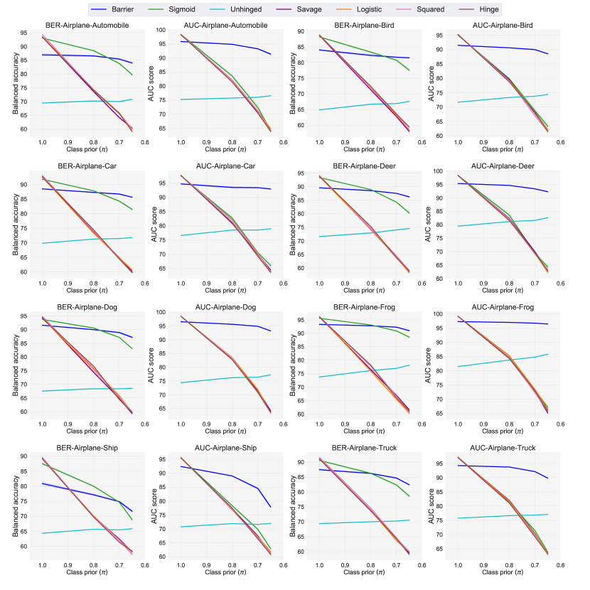
Figure 6: Mean balanced accuracy (1-BER) and AUC score using convolutional neural networks (rescaled to 0-100). The noise rate is ranged from $(\pi=1.0,\pi^{\prime}=0.0),(\pi=0.8,\pi^{\prime}=0.3),(\pi=0.7,\pi^{\prime}=0.4),(\pi=0.65,\pi^{\prime}=0.45)$.

Figure 7: Mean balanced accuracy (1-BER) and AUC score using convolutional neural networks (rescaled to 0-100). The noise rate is $\pi=0.65$ and $\pi^{\prime}=0.45$. The experiments were conducted 10 times.

References

• Aslam & Decatur (1996) Aslam, J. A. and Decatur, S. E. On the sample complexity of noise-tolerant learning. Information Processing Letters, 57(4):189–195, 1996.
• Bao et al. (2018) Bao, H., Niu, G., and Sugiyama, M. Classification from pairwise similarity and unlabeled data. In ICML, pp.  452–461, 2018.
• Bartlett & Tewari (2007) Bartlett, P. L. and Tewari, A. Sparseness vs estimating conditional probabilities: Some asymptotic results. JMLR, 8:775–790, 2007.
• Bartlett et al. (2006) Bartlett, P. L., Jordan, M. I., and McAuliffe, J. D. Convexity, classification, and risk bounds. JASA, 101(473):138–156, 2006.
• Ben-David et al. (2003) Ben-David, S., Eiron, N., and Long, P. M. On the difficulty of approximately maximizing agreements. Journal of Computer and System Sciences, 66(3):496–514, 2003.
• Biggio et al. (2011) Biggio, B., Nelson, B., and Laskov, P. Support vector machines under adversarial label noise. In ACML, pp.  97–112, 2011.
• Blanchard et al. (2010) Blanchard, G., Lee, G., and Scott, C. Semi-supervised novelty detection. JMLR, 11:2973–3009, 2010.
• Buja et al. (2005) Buja, A., Stuetzle, W., and Shen, Y. Loss functions for binary class probability estimation and classification: Structure and applications. Working draft, 2005.
• Cesa-Bianchi et al. (1999) Cesa-Bianchi, N., Dichterman, E., Fischer, P., Shamir, E., and Simon, H. U. Sample-efficient strategies for learning in the presence of noise. Journal of the ACM, 46(5):684–719, 1999.
• Chang & Lin (2011) Chang, C.-C. and Lin, C.-J. LIBSVM: a library for support vector machines. ACM Transactions on Intelligent Systems and Technology, 2(3):27, 2011.
• Cheng et al. (2002) Cheng, J., Hatzis, C., Hayashi, H., Krogel, M.-A., Morishita, S., Page, D., and Sese, J. KDD Cup 2001 report. ACM SIGKDD Explorations Newsletter, 3(2):47–64, 2002.
• Chow (1970) Chow, C. K. On optimum recognition error and reject tradeoff. IEEE Transactions on Information Theory, 16(1):41–46, 1970.
• du Plessis et al. (2014) du Plessis, M. C., Niu, G., and Sugiyama, M. Analysis of learning from positive and unlabeled data. In NeurIPS, pp.  703–711, 2014.
• du Plessis et al. (2015) du Plessis, M. C., Niu, G., and Sugiyama, M. Convex formulation for learning from positive and unlabeled data. In ICML, pp.  1386–1394, 2015.
• Feldman et al. (2012) Feldman, V., Guruswami, V., Raghavendra, P., and Wu, Y. Agnostic learning of monomials by halfspaces is hard. SIAM Journal on Computing, 41(6):1558–1590, 2012.
• Gao & Zhou (2015) Gao, W. and Zhou, Z.-H. On the consistency of auc pairwise optimization. In IJCAI, pp.  939–945, 2015.
• Ghosh et al. (2015) Ghosh, A., Manwani, N., and Sastry, P. Making risk minimization tolerant to label noise. Neurocomputing, 160:93–107, 2015.
• Ghosh et al. (2017) Ghosh, A., Kumar, H., and Sastry, P. Robust loss functions under label noise for deep neural networks. In AAAI, pp.  1919–1925, 2017.
• Guyon et al. (2005) Guyon, I., Gunn, S., Ben-Hur, A., and Dror, G. Result analysis of the NIPS 2003 feature selection challenge. In NeurIPS, pp.  545–552, 2005.
• Ishida et al. (2017) Ishida, T., Niu, G., Hu, W., and Sugiyama, M. Learning from complementary labels. In NeurIPS, pp.  5639–5649, 2017.
• Ishida et al. (2018) Ishida, T., Niu, G., and Sugiyama, M. Binary classification from positive-confidence data. In NeurIPS, pp.  5917–5928, 2018.
• Kiryo et al. (2017) Kiryo, R., Niu, G., du Plessis, M. C., and Sugiyama, M. Positive-unlabeled learning with non-negative risk estimator. In NeurIPS, pp.  1674–1684, 2017.
• Krizhevsky & Hinton (2009) Krizhevsky, A. and Hinton, G. Learning multiple layers of features from tiny images. Technical report, Citeseer, 2009.
• LeCun (1998) LeCun, Y. The mnist database of handwritten digits. http://yann. lecun. com/exdb/mnist/, 1998.
• Lichman et al. (2013) Lichman, M. et al. UCI machine learning repository, 2013.
• Long & Servedio (2010) Long, P. M. and Servedio, R. A. Random classification noise defeats all convex potential boosters. Machine learning, 78(3):287–304, 2010.
• Lu et al. (2018) Lu, N., Niu, G., Menon, A. K., and Sugiyama, M. On the minimal supervision for training any binary classifier from only unlabeled data. arXiv preprint arXiv:1808.10585, 2018.
• Manwani & Sastry (2013) Manwani, N. and Sastry, P. Noise tolerance under risk minimization. IEEE Transactions on Cybernetics, 43(3):1146–1151, 2013.
• Masnadi-Shirazi & Vasconcelos (2009) Masnadi-Shirazi, H. and Vasconcelos, N. On the design of loss functions for classification: theory, robustness to outliers, and savageboost. In NeurIPS, pp.  1049–1056, 2009.
• Menon et al. (2015) Menon, A., van Rooyen, B., Ong, C. S., and Williamson, B. Learning from corrupted binary labels via class-probability estimation. In ICML, pp.  125–134, 2015.
• Menon & Williamson (2016) Menon, A. K. and Williamson, R. C. Bipartite ranking: a risk-theoretic perspective. JMLR, 17(1):6766–6867, 2016.
• Nair & Hinton (2010) Nair, V. and Hinton, G. E. Rectified linear units improve restricted boltzmann machines. In ICML, pp.  807–814, 2010.
• Narasimhan & Agarwal (2013) Narasimhan, H. and Agarwal, S. On the relationship between binary classification, bipartite ranking, and binary class probability estimation. In NeurIPS, pp.  2913–2921, 2013.
• Natarajan et al. (2013) Natarajan, N., Dhillon, I. S., Ravikumar, P. K., and Tewari, A. Learning with noisy labels. In NeurIPS, pp.  1196–1204, 2013.
• Niu et al. (2016) Niu, G., du Plessis, M. C., Sakai, T., Ma, Y., and Sugiyama, M. Theoretical comparisons of positive-unlabeled learning against positive-negative learning. In NeurIPS, pp.  1199–1207, 2016.
• Paszke et al. (2017) Paszke, A., Gross, S., Chintala, S., Chanan, G., Yang, E., DeVito, Z., Lin, Z., Desmaison, A., Antiga, L., and Lerer, A. Automatic differentiation in pytorch. 2017.
• Reddi et al. (2018) Reddi, S. J., Kale, S., and Kumar, S. On the convergence of Adam and beyond. In ICLR, 2018.
• Reid & Williamson (2010) Reid, M. D. and Williamson, R. C. Composite binary losses. JMLR, 11:2387–2422, 2010.
• Sakai et al. (2018) Sakai, T., Niu, G., and Sugiyama, M. Semi-supervised auc optimization based on positive-unlabeled learning. Machine Learning, 107(4):767–794, 2018.
• Scott (2015) Scott, C. A rate of convergence for mixture proportion estimation, with application to learning from noisy labels. In AISTATS, pp.  838–846, 2015.
• Scott et al. (2013) Scott, C., Blanchard, G., and Handy, G. Classification with asymmetric label noise: Consistency and maximal denoising. In COLT, pp.  489–511, 2013.
• Srivastava et al. (2014) Srivastava, N., Hinton, G., Krizhevsky, A., Sutskever, I., and Salakhutdinov, R. Dropout: a simple way to prevent neural networks from overfitting. JMLR, 15(1):1929–1958, 2014.
• Tokui et al. (2015) Tokui, S., Oono, K., Hido, S., and Clayton, J. Chainer: a next-generation open source framework for deep learning. In NeurIPS Workshop, volume 5, 2015.
• van Rooyen et al. (2015a) van Rooyen, B., Menon, A., and Williamson, R. C. Learning with symmetric label noise: The importance of being unhinged. In NeurIPS, pp.  10–18, 2015a.
• van Rooyen et al. (2015b) van Rooyen, B., Menon, A. K., and Williamson, R. C. An average classification algorithm. arXiv preprint arXiv:1506.01520, 2015b.
• Yuan & Wegkamp (2010) Yuan, M. and Wegkamp, M. Classification methods with reject option based on convex risk minimization. JMLR, 11:111–130, 2010.
• Zhang (2004) Zhang, T. Statistical behavior and consistency of classification methods based on convex risk minimization. Annals of Statistics, pp.  56–85, 2004.
• Zhou (2017) Zhou, Z.-H. A brief introduction to weakly supervised learning. National Science Review, 5(1):44–53, 2017.