A Structured Approach to the Analysis of Remote Sensing Images

Abstract

The number of studies for the analysis of remote sensing images has been growing exponentially in the last decades. Many studies, however, only report results—in the form of certain performance metrics—by a few selected algorithms on a training and testing sample. While this often yields valuable insights, it tells little about some important aspects. For example, one might be interested in understanding the nature of a study by the interaction of algorithm, features, and the sample as these collectively contribute to the outcome; among these three, which would be a more productive direction in improving a study; how to assess the sample quality or the value of a set of features etc. With a focus on land-use classification, we advocate the use of a structured analysis. The output of a study is viewed as the result of the interplay among three input dimensions: feature, sample, and algorithm. Similarly, another dimension, the error, can be decomposed into error along each input dimension. Such a structural decomposition of the inputs or error could help better understand the nature of the problem and potentially suggest directions for improvement. We use the analysis of a remote sensing image at a study site in Guangzhou, China, to demonstrate how such a structured analysis could be carried out and what insights it generates. The structured analysis could be applied to a new study, or as a diagnosis to an existing one. We expect this will inform practice in the analysis of remote sensing images, and help advance the state-of-the-art of land-use classification.

1 Introduction

The number of studies for the analysis of remote sensing images has been increasing exponentially in the last decades. Many studies, however, only report results—in the form of certain performance metrics—by a few selected algorithms on a training and testing sample. While this often provides valuable insights to practitioners, it tells little about several important aspects. For example, one might be interested in understanding a study by the interaction among algorithms, features, and the sample. This is important, as these are the factors in a study that involve human decisions which collectively contribute to the outcome of the study. Also of interest is to find out a possible direction for further work in improving an existing study—will it be more productive to work really hard on the algorithm, or just focus on finding better features, or simply increase the sample size? How much value will it add to increase the sample size? This last question arises increasingly often as, after years of practice, the accumulated sample may already be fairly large and it is interesting to know if further data collection is worthwhile. Additionally, one might be interested in assessing the value of features to decide which features to pursue in a future study, or the sample quality to see if the collection procedure needs to be improved.

To shed lights into various important aspects of a study, we advocate the use of a structured analysis. We will introduce our approach, particularly, for the land-use classification problem. Our idea was inspired by regression diagnosis in statistics [2, 9]. Regression diagnosis refers to the assessment of regression analysis, including the validation of various statistical assumptions made in regression analysis, the evaluation of variables used in the model, and an examination of the influence of individual data points to the model. To better align with the particular goals of land-use classification, we re-orient the focus of our structured analysis. While regression diagnosis seeks to validate and understand regression results, we aim at a better understanding of studies in land-use classification and to identify potential spots for further improvement.

We take a structured approach. This is to overcome the complexity of the land-use classification problem—a number of factors contribute to the outcome and some may interact with others in a complicated way. We start by treating the land-use classification as a system with inputs and output. The output is the outcome under some metrics, for example the error rate. The inputs are factors that contribute to the outcome, which we identify as three interplaying entities: feature, sample, and algorithm. We term these three entities as the three degrees of freedom (or dimension) of a study. Here, feature refers to the set of features (variables) included in a study, such as vegetation index, quantities describing the texture pattern in a remote sensing image, values on some spectral bands etc. Sample are collected instances of the tuple, in the form of $(x_{1},x_{2},...,x_{p},y)$, where $x_{i}$ is the value of the i-th feature, $i=1,2,...,p$, and $y$ is the land-use type. Algorithm is the type of classifiers or models one chooses to use, such as linear models or decision trees etc.

We view the error as the fourth dimension of a study. Error can happen to any of the other three dimensions (i.e., feature, sample, and algorithm). Distinguishing those can help better understand the study, and to trace the contributing source to the outcome. Now that we have identified individual components in a study, how to put those together to form a system and to interpret the outcome? That is our structured analysis model, to be discussed in detail in Section 2.

A structured analysis will help understand studies in land-use classification. It would yield information that connects the dimensions of a study and the observed outcome. Such information could help us better understand the results, and potentially suggest directions on how to improve the study of land classification. We will use the analysis of a remote sensing image about a study site in Guangzhou, China, to demonstrate how a structured analysis could be carried out. We expect this will inform practice in the analysis of remote sensing images, and help advance the state-of-the-art of study on the land classification problem.

It is worthwhile to mention [27], a compressive study involving over a dozen of different classification algorithms with varying sample sizes. This work gives valuable insights to the practice of land classification, including the the importance of sufficient training samples and sample quality etc. In contrast, our approach was inspired by regression diagnosis and builds on the theory of pattern classification. It can be used as a general framework for the analysis of a particular study site, or to understand, evaluate, or improve various aspects of an existing analysis (thus could be viewed as a meta analysis). Our approach considers all important aspects in a land-use classification analysis, including their interactions and tradeoff etc, and gives methodological guideline to practice. While there are common elements with [27] on the assessment of training samples and algorithms, we delve further and towards broader issues. Our approach helps to decide if the training samples are sufficient, if the algorithms used are rich enough to capture the patterns in the particular land-use problem, how to assess or compare the importance of features, what are the difficult land-use types to classify, what are the possible, or most profitable, directions (among sample, feature, or algorithm) to work on for further improvement of a study etc.

2 A model for structured analysis

In this section, we will introduce our model for structured analysis. To make the model more interpretable, we include ground truth, and two additional ‘virtual’ entities: the probability distribution and the Bayes rule. By ‘virtual’ we mean entities not observable, but are fundamental in land-use classification. Figure 1 is an illustration of our model. Note that the three rectangles indicate entities that involve one’s choices and decisions, while entities enclosed by a dashed oval are virtual entities. For the rest of this section, we will explain individual entities in the model.

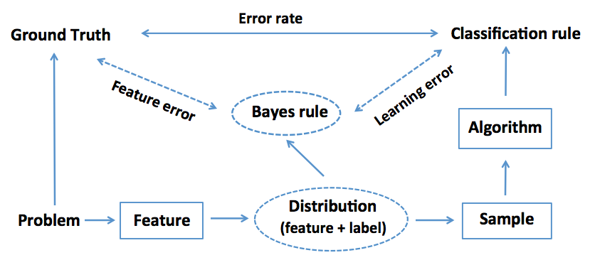
Figure 1: A model for structured analysis.

The probability distribution tells how the values of the (feature, label) pair, denoted by $({\bm{X}},Y)$, look like in the data space. It is decided by the features (i.e., variables) used in the study and the nature of the given land-use classification problem. The distribution determines the actual classification problem we work with, and, consequently, the lowest possible error rate achievable by any classifiers, i.e., the Bayes rate. The classifier that achieves the Bayes rate is called a Bayes rule. Once the set of features is chosen, the Bayes rate is the theoretical lowest possible error rate one can achieve, regardless of how hard one works on improving the classification algorithm or how big the training sample is.

For every land-use classification problem, there is a ground truth, which always tells the correct label. When one chooses to use a particular set of features in a study, there is often a loss of information (since there are other features potentially informative but not used). This would cause a gap between the Bayes rule and ground truth. We call this feature error. To reduce the gap, one needs to improve on feature selection.

The idea of classification is to find a mapping $f$ between the feature $\bm{X}$ and the label $Y$. This requires knowledge about the probability distribution, which is generally unknown; what we have is a sample collected from this distribution. We wish to use the sample to estimate the mapping $f$; the estimated mapping $\hat{f}$ is called a classification rule. The sample size can be changed, depending on the availability. Often, a large sample is desired. However, after certain point, the gain in performance diminishes when further increasing the sample size.

Now given a collected sample, we need an algorithm to fit a classification rule (i.e., to find the estimated mapping $\hat{f}$). By algorithm we mean the type of classifiers or models, such as linear models or decision trees etc, used to fit the classification rule. Different choices of algorithms lead to different types of classification rules. The fitted classification rule will be used for classification on the test sample. With reference to the ground truth, one can calculate the error rate, which is the proportion of the test sample that receives a wrong label.

2.1 The errors in the structured analysis model

The errors play an important role in our model of structured analysis. While the classification error rate measures the final outcome, it is a little crude. It will be helpful to decompose the classification error according to the error sources. There are three sources of errors, corresponding to feature error, sample error, and learning error, respectively. We have discussed the feature error, next we will discuss sample error and learning error.

The learning error results from the training of the classifier. In practice, we know neither $f$ nor the probability distribution. We wish to use a training sample collected from the unknown distribution to learn the classification rule with some algorithm. There are two potential errors. One is the approximation error due to the inappropriate choice of the type of algorithms. For example, for a particular problem, a boosting [16] type of algorithms work the best but support vector machine [10] or a simple linear model is used. Another is called the convergence error, due to the insufficient size of the training sample. One could lower the convergence error by increasing the sample size, while the approximate error could be reduced by increasing the richness of the family of classification rules in model fitting (one could try different algorithms when there is not much information about the problem structure).

The sample error refers to the discrepancy between the true probability distribution of $({\bm{X}},Y)$ and that of the collected sample. It is related to the data quality or whether the sample is representative of the true probability distribution. The representativeness of the sample is related to the study design. Usually the principle of random sampling [32] is followed. There are generally two types of errors related to data quality, namely, data perturbation [46, 25, 30] and data contamination [38, 46, 40]. Data perturbation is often caused by additive noise and would affect a large proportion of the data, typically at a small amount. Data contamination substitutes a random subset of the data by a different distribution. Both will impact the accuracy of the land classification.

On an orthogonal direction, one may decompose the error according to the land types. Which land-use types are frequently misclassified? Or misclassified into which land-use types? This could be done with a confusion matrix to be discussed in Section 4.2. Such information would become useful clues in the search of better algorithms or new features.

3 Study site and the data

Our study site is located in the Pearl River Delta, or more specifically, the region spanning 23°2’-23°25’N, 113°8’-113°35’E, in Guangdong Province of South China. The study site contains the central part of Guangzhou and its rural-urban fringe. Figure 2 is a Landsat Thematic Mapper (TM) image for the study site. As Guangzhou has undergone rapid urban development in the last two decades, it has been studied extensively for land use, land cover mapping and change detection; see, for example, [33, 14, 13, 27].

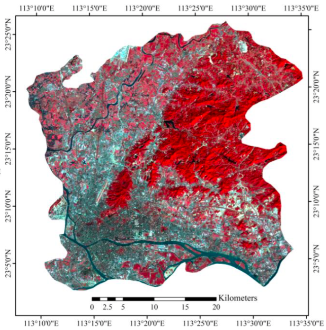
Figure 2: The study area. The image displays the green, red and near infrared band of the TM data with blue, green, and red colour guns.

The Landsat TM image for the study site was acquired on 2 January 2009, in the dry season of this area. The raw imagery was geo-referenced in 2005 with a root mean squared error of 0.44 pixels. A 6-band set of the TM data was used (excluding the thermal band due to its coarse resolution).

With reference to some popular land cover and land-use classification systems [19, 20, 21, 27], 7 different land-use types (a.k.a. classes) are used in our study. A brief description of the land-use types is given in Table 1.

Land-use type	Description
Water	Water bodies such as reservoirs, ponds and river
Residential area	Areas where driveways and roof tops dominate
Natural forest	Large area of trees
Orchard	Large area of fruit trees
Industrial/commercial	Lands where roof tops of large buildings dominate
Idle land	Lands where no vigorous vegetation grows
Bareland	Lands where vegetation is denuded or where the
	construction is underway

Table 1: A description of 7 different land-use types.

The training and test samples are adopted from a recent study [27]. The training sample size is 2880, and the number of instances are $240,240,480,240,960,240,480$, respectively, for the 7 land-use types in the order listed in Table 1. The test sample has a size of 423, with a class distribution of

$$(9.69\%,21.51\%,19.62\%,11.35\%,16.78\%,10.64\%,10.40\%).$$

We use the classification error as the evaluation metric as this is common in the data mining and also the remote sensing literature (note another popular metric is the Kappa statistic); also we will use a quantity, the distance of separation to be discussed in Section 4 to assess the relative strength of different features.

We use a total of 56 features. There are 6 spectral features corresponding to the 6 TM bands, including blue, green, red, near infrared, shortwave infrared 1, and shortwave infrared 2, respectively. Each TM band corresponds to 8 texture features, including mean, variance, homogeneity, contrast, dissimilarity, entropy, second moment, correlation; this gives a total of 48 texture features. Additionally, there are two location features, the latitude and longitude of the ground position associated with each data instance. Table 2 is a summary of the features.

Feature code	Description
Lat, Lon	Latitude, longitude
B1, B2, …, B6	Spectral features for the 6 TM bands
B7, B8, …, B54	Texture features. Each of the 6 TM bands
	corresponds to 8 texture features

Table 2: A list of all features used (totally 56). The texture features for each of the 6 bands are listed in the order of mean, variance, homogeneity, contrast, dissimilarity, entropy, second moment, and correlation.

4 Tools for structured analysis

In a land-use classification study, we are often interested in several important questions. How good is a particular set of features? What might be the contribution of individual features? Will it add value, or how much value would it be, by adding another set of new features? What would one expect on the predictive accuracy from the ‘best’ algorithm if he has ‘enough’ computing power and sample? Which land-use types are more prune to classification errors? To gain insights into these questions, we propose to study several quantities, including the covariance matrix of the features, the confusion matrix of errors, and the distance of separation of the data (under a given set of features). For the rest of this section, we will introduce these along with a characterization on when combining two sets of features may be beneficial.

4.1 The covariance matrix

For a given set of features, a central quantity in characterizing the data distribution is the covariance structure of the features. This is described by the covariance matrix, denoted by $\bm{\Sigma}$, with its $(i,j)$-position defining the covariance between the $i^{th}$ and $j^{th}$ feature. That is,

$$\bm{\Sigma}_{i,j}=\mathbb{E}(X^{i}-{\mu}^{i})(X^{j}-\mu^{j}),$$ (1)

where $\mathbb{E}$ indicates expectation, $\mu^{i}$ and $\mu^{j}$ are the mean of the $i^{th}$ and $j^{th}$ feature which are denoted by $X^{i}$ and $X^{j}$, respectively. In practice, one often scale each feature to have a variance 1 and this leads to the correlation matrix. To abuse the notation a bit, we still use $\bm{\Sigma}$ for the correlation matrix. All entries of the correlation matrix are in the range $[-1,1]$. A small $|\bm{\Sigma}_{i,j}|$ indicates a low correlation between the $i^{th}$ and $j^{th}$ feature; otherwise there would be a collinearity among features and special cares (e.g., regularization) are needed in model fitting. If the features jointly follow a normal distribution, then $|\bm{\Sigma}_{i,j}|=0$ is equivalent to the independence of the two features.

4.2 The confusion matrix

The confusion matrix [37] is a two-way table that summarizes the test instances according to their actual class and predicted class. It has the following form:

	1	…	j	…	C	Total
1	$n_{11}$	…	$n_{1j}$	…	$n_{1C}$	$n_{1.}$
…	…	…	…	…	…	…
i	$n_{i1}$	…	$n_{ij}$	…	$n_{iC}$	$n_{i.}$
…	…	…	…	…	…	…
C	$n_{C1}$	…	$n_{Cj}$	…	$n_{CC}$	$n_{C.}$
Total	$n_{.1}$	…	$n_{.j}$	…	$n_{.C}$	n

where the columns indicate the true land-use types (classes) and the rows predicted ones, C is the number of different classes, $n_{ij}$ is the number of instances from class $i$ but classified as being from class $j$, $n_{i.}$’s are the row sums and $n_{.j}$’s are the column sums of the table, and $n$ is the size of the test sample. The numbers on the diagonal are the instances correctly classified while off-diagonals are misclassified. The confusion matrix allows one to see where the errors are by classes. This will help narrow down the focus to a few hard to classify land-use types, and suggest directions for further study.

4.3 The distance of separation

The distance of separation was studied by [42] as an indication of the strength of a set of features. The associated theoretical model is the Gaussian mixture, due to it versatility in modeling the real data [29]. For simplicity, we consider the 2-component Gaussian mixture specified as

$$\Theta\mathcal{N}(\bm{\mu},\bm{\Sigma})+(1-\Theta)\mathcal{N}(-\bm{\mu},\bm{\Sigma}),$$ (2)

where $\Theta\in\{0,1\}$ indicates the label of an observation such that $\mathbb{P}(\Theta=1)=\theta$, and $\mathcal{N}(\bm{\mu},\bm{\Sigma})$ stands for Gaussian distribution with mean $\bm{\mu}\in\mathbb{R}^{p}$ and covariance matrix $\bm{\Sigma}$. Here W.L.O.G., we assume the center of the mixture components are $\pm\bm{\mu}$. This can be achieved by shifting the data without changing the nature of the problem. For simplicity, we consider $\theta=\frac{1}{2}$ and the 0-1 loss.

The distance of separation is defined as

$$d_{\bm{\mathcal{F}}}=\bm{\mu}_{\bm{\mathcal{F}}}^{T}\bm{\Sigma}^{-1}\bm{\mu}_{\bm{\mathcal{F}}},$$ (3)

where $\bm{\mathcal{F}}$ indicates a set of features, $\bm{\Sigma}$ and $\pm\bm{\mu}$ are as defined in (2). At an intuitive level, one can view $d_{\bm{\mathcal{F}}}$ as indicating how far apart the data is between different classes—the larger this distance is, the data are further apart thus easier for a classification algorithm to locate the class boundary. It is related to the Bayes error of classification for which there is a well-known result.

Lemma 4.1 ([1, 12]).

For Gaussian mixture (2) and 0-1 loss, the Bayes error rate is given by $\Phi(-\frac{1}{2}(\bm{\mu}_{\bm{\mathcal{F}}}^{T}\bm{\Sigma}^{-1}\bm{\mu}_{\bm{\mathcal{F}}})^{1/2})$ where $\Phi(\cdot)$ is defined as $=\int_{-\infty}^{x}\frac{1}{\sqrt{2\pi}}e^{-\frac{z^{2}}{2}}dz$.

To better appreciate the role played by the distance of separation in Bayes error, we plot in Figure 3 the Bayes error as a function of the distance of separation. It can be seen that the Bayes error decreases exponentially fast as the distance of separation increases.

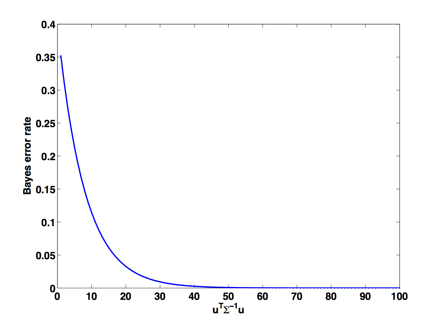
Figure 3: Bayes error rate as a function of the distance of separation.

The connection between the distance of separation and Bayes error allows us to quantify the ‘strength’ of a feature set. The larger the distance of separation, the smaller the Bayes error (by Lemma 4.1), and consequently, the smaller the feature error (as the ground truth is always correct) by Figure 1. It should be noted, however, that to translate the strength of a feature set to empirical performance, the training sample size needs to grow proportionally and the classifier is rich enough to match the complexity of the problem.

Additionally, when using the empirical distance of separation, one should keep in mind that such an estimate would only serve the purpose of giving a qualitative characterization rather than quantifying the actual Bayes error. The is because it involves the estimation of the covariance matrix which is notoriously difficult when the number of features is large [3, 15].

4.4 The marginal benefit

One can also use the distance of separation to study the marginal benefit of one set of features w.r.t. another. If new features cause the distance of separation to increase thus a smaller Bayes error, then it is beneficial to add such new features. Again, a sufficiently large training sample size is required for the reduced Bayes error to materialize; otherwise, it may be harmful to the empirical performance due to a potential overfit caused by the small sample size.

In this section, we will characterize a situation where the inclusion of a set of new features will be marginally beneficial. Roughly, we require the set of new features to posses discriminative power and that the two sets of features have ‘low’ dependence. The discriminative power is equivalent to a positive distance of separation, as a 0 distance of separation would result in a random guess, i.e., 50% Bayes error for a two-class classification problem.

Let the covariance matrix $\bm{\Sigma}$ be written as

$$\bm{\Sigma}=\left[\begin{array}[]{cc}\bm{A}_{11}&\bm{A}_{12}\\ \bm{A}_{12}^{T}&\bm{A}_{22}\\ \end{array}\right]$$

where we assume block $\bm{A}_{11}$ and $\bm{A}_{22}$ correspond to two sets of features, respectively, after a permutation of rows and columns of $\bm{\Sigma}$. Correspondingly, write $\bm{u}_{\bm{\mathcal{F}}}=[\bm{u}_{1},\bm{u}_{2}]^{T}$ and $\bm{\mathcal{F}}=[\bm{\mathcal{F}}_{1},\bm{\mathcal{F}}_{2}]^{T}$. We assume $||\bm{A}_{12}||_{F}=o(1)$ for a ‘low’ dependence between two sets of features $\bm{\mathcal{F}}_{1}$ and $\bm{\mathcal{F}}_{2}$; here $||.||_{F}$ denotes the Frobenius norm [18] and $o(1)$ is the little-o notation indicating that the quantity is small compared to 1. Our main result can be stated as the following theorem.

Theorem 4.2.

Suppose the data is generated according to (2). Assume $\bm{u}_{2}^{T}\bm{A}_{22}^{-1}\bm{u}_{2}>c>0$, $||\bm{A}_{12}||_{F}=o(1)$, $||\bm{u}||_{F}\leq C$ for some positive constants $c$ and $C$, and that the eigenvalues of both $\bm{A}_{11}$ and $\bm{A}_{22}$ are bounded away from $0$ and $\infty$. Then

$$\bm{u}_{\bm{\mathcal{F}}}^{T}\bm{\Sigma}^{-1}\bm{u}_{\bm{\mathcal{F}}}>\bm{u}_{1}^{T}\bm{A}_{11}^{-1}\bm{u}_{1}.$$ (4)

The proof of Theorem 4.2 follows a similar line of arguments as [42], and is given in the appendix. Rather than discussing the technical details, we will give here a few remarks on the interpretation and implication of Theorem 4.2.

Remarks. 1). It is beneficial to combine two sets of features with low correlation (provided that the training sample is sufficiently large and the family of classifiers is rich enough). The theorem states that this would lead to a larger distance of separation thus a decreased Bayes error.
2). Setting $||\bm{A}_{12}||_{F}=0$ recovers the independence case. So the independence case is a special case of Theorem 4.2.
3). Extra features will not help much if the existing features are already good enough, i.e., $\bm{u}_{1}^{T}\bm{A}_{11}^{-1}\bm{u}_{1}$ is big. In such a case, the Bayes error under the existing features is already very small, and there is not much room for improvement.

5 Methods

Our implementation of a structured analysis focus on the four dimensions of a study, including sample, algorithm, feature, and the error, as well as a decomposition of the error by the confusion matrix. We will discuss each in this section.

5.1 Sample

The sample is an important dimension in a study. While we have decoupled the feature aspect from the data (c.f. Section 2), there remain several aspects of importance (assuming the data has been properly cleaned and pre-processed). These include the size, quality, and representativeness of the data.

The size of the sample is related to the convergence error in model fitting. Typically, a larger sample would improve the predictive accuracy, but often that is not feasible in practice. Also, one may wish to know how much improvement to expect when there is a larger sample. We propose to subsample the training set at varying sizes to see the trend of the error rate vs the training sample size. This will help probe the convergence error, and to see if a larger sample will likely lead to a notable improvement in the performance.

Additionally, when inspecting the confusion matrix, we suggest subsample the training set to extrapolate how the confusion matrix will change when the sample size increases. Of particular interests are those cells, or rows, in the confusion matrix indicating a substantially higher error rate than others. These will allow us to focus on those challenging land-types, and we can then examine if the algorithm or the features are adequate for those land-types.

To assess the data quality or representativeness of the sample is a hard problem, as the true probability distribution is unknown. For the particular sample used in this study, it is possible to carry out hypothesis testing according to the ground position (latitude and longitude) associated with a pixel. That is, to test whether the set of (latitude, longitude) pairs from the sample have a uniform distribution over the study region. However, that would require the (latitude, longitude) information, and that the study region has a regular shape (so that it would be easy to do computation), which are typically not applicable in other studies, we omit the discussion here.

For land classification problems, feature noises are mainly caused by noises to the remote sensing images. Fortunately, the advance in remote sensing technology has now made it much less of a concern than the label noise. So here we focus on the label noise and its potential impact. It is in general hard to estimate the amount of label noise, we suggest the following procedure to probe it. Randomly select a proportion, $\epsilon\in[0,1]$, of data and then flip the labels uniformly at random to a different label. The prediction error on the clean (uncontaminated) test set for each $\epsilon$ form a curve of test errors vs $\epsilon$. This curve allows us to extrapolate the amount of label noise in the original sample or its impact. $\epsilon$ is estimated to be smaller than 10% in many applications according to [23]. We recommend trying several different classification algorithms, particularly Random Forests (RF, [4]) which has a reputation of strong noise resistance. If the curves by different classifiers are all steep, that is an indication of potentially non-negligible label noise; if at least one curve is relatively flat, then either the label noise is small or its impact can be safely ignored.

5.2 Algorithms

The algorithm is another dimension of a study. It is related mainly to the approximation error in model fitting. The richness of the family of classifiers is required to ‘match’ the complexity of the classification problem in order to have a small approximation error. The complexity of the problem is determined by the distribution of $({\bm{X}},Y)$, which is often unknown. To probe this, we recommend trying several different types of algorithms, hoping that some would have a matching richness. A number of existing studies [43, 27] are actually along this line. Of course, different types of algorithms may have a different convergence rate (faster convergence implies a smaller convergence error for a given sample size). Here convergence indicates that the classification algorithm has reached a state that further increasing the sampling size will no longer cause much changes to the classification rule. When the sample size is ‘small’, it is highly desirable to explore a range of different types of algorithms.

Since many different algorithms have already been explored in [27], we choose to use two of best performing ones, RF and $L_{1}$-regularized logistic regression [17]. RF is widely acknowledged as one of the most powerful tools in statistics and machine learning according to some empirical studies [4, 7, 6]. Regularized logistic regression is a popular algorithm that combines a superior predictive performance with a strong variable selection capability.

RF is an ensemble of decision trees. Each tree is built by recursively partitioning the data. At each node (the root node corresponds to the bootstrap sample), RF randomly samples (with replacement) a number of features and then select one for an ‘optimal’ partition of that node. This process continues recursively until the tree is fully grown, that is, only one data point is left at each leaf node. RF often has superior empirical performance, is very easy to use (e.g., very few tuning parameters) and show a remarkable built-in ability for feature selection. We will use the R package randomForest.

Logistic regression models the log odds ratio of the posterior probability as a linear function of the co-variates (i.e., features):

$$log\frac{P(Y=1|\bm{X}=\bm{x})}{1-P(Y=1|\bm{X}=\bm{x})}=\sum_{i=1}^{p}\beta_{i}x_{i},$$ (5)

where $\bm{x}=(x_{1},...,x_{p})$. When there is a potential high collinearity among the features, and, especially when the number of features is large w.r.t. the sample size, typically regularization is used. Regularization [36] is the idea of injecting external knowledge, e.g., smoothness [26, 39] or sparsity [8, 11, 35] etc, into model fitting. A popular form of regularization is to enforce an $L_{1}$-penalty on the coefficients [35, 31, 17]. This leads to the following $L_{1}$-regularized logistic regression:

$$\arg\max_{\beta=(\beta_{1},...\beta_{p})}L(\beta)=\Pi_{i=1}^{n}\left[p(\bm{X}_{i})\right]^{Y_{i}}\left[1-p(\bm{X}_{i})\right]^{1-Y_{i}}+\lambda\sum_{i=1}^{p}|\beta_{i}|,$$ (6)

where $\lambda$ is a regularization parameter. Often (6) leads to a compact model with a ‘good’ predictive accuracy. We will use the R package glmnet [17].

5.3 Features

Perhaps the most important dimension of a study is the feature, as it determines the classification problem for subsequent analysis. In our structured analysis model, the features are related to the feature error. A careful examination of the features can help gauge its strength, thus give insights on whether it is worthwhile to work further on feature extraction, or to improve the algorithm, or simply try to get a larger sample. It would also help in comparing two sets of features, or to give clues on the marginal benefit of a set of new features. Among our tools for examining the features are the covariance matrix, the distance of separation, and feature importance profiling etc.

Our assessment of the features consists of an inspection on the covariance matrices, the computation of the distance of separation for relevant features, the generation of a feature importance profile, and, possibly, feature selection. As we have discussed the covariance matrix and the distance of separation in Section 4, here we only discuss feature importance while omitting feature selection as it is too big a topic (readers can refer to [28, 22, 34] and references therein).

We recommend the use of RF to produce a feature importance profile. There are two feature importance metrics in RF, one based on the Gini index and the other permutation accuracy [5, 4]. We consider the later here, as it is often considered superior. The idea is as follows. Randomly permute the values of a feature, say, the $i^{th}$ feature, then its association with the response $Y$ is broken. When this feature, along with those un-permuted features, is used for prediction, the accuracy tends to decrease. The difference in the prediction accuracy before and after permuting the $i^{th}$ feature can then be used as a measure of its importance.

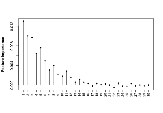
Figure 4: Feature importance by RF for the given example.

In the following, we use a two-component Gaussian mixture as an example to demonstrate the use of RF for feature importance profiling. The Gaussian mixture is defined as in (2) with

$$\bm{\mu}=(0.2,0.19,0.18,...,0.01,0,0,...0)\in\mathbb{R}^{30},\bm{\Sigma}_{i,j}=0.1^{|i-j|}.$$

Thus the importance of features decreases with their feature index, with the last 10 features being purely noise features. Figure 4 shows the importance of features, ordered by their indices. It can be seen the feature importance as produced by RF agrees fairly well with the generating model.

6 Results

In our experiments, we study the land-use classification using a study site in the Pearl River Delta region. Our experiments center around the four dimensions of a study. We explore a number of important aspects of land-use classification with structured analysis. This includes a study on the predictive accuracy of a classifier with varying sample sizes, marginal benefits of spectral, textural or location features, feature importance profiling, which land-use types are more difficult to classify than others, and predictive performance under ‘small’ sample size. This is different from usual studies in remote sensing which usually focus on the prediction accuracy.

Experiments	Results	Dimension of relevance
Sample size and performance	Figure 5	Sample, algorithm, features
Label noise	Figure 6	Error, sample, algorithm
Small sample performance	Figure 9	Sample, algorithm, features
Marginal benefits	Figure 7	Features
	Figure 5	Features
Distance of separation	Figure 7	Features
Covariance matrix	Figure 8	Features
Feature importance	Figure 10	Features, algorithm
Confusion matrix	Table 4	Error, algorithm, features
Difficult land-types	Figure 11	Error, sample, features
	Figure 12	Error, sample, features
	Figure 13	Error, sample, algorithm

Table 3: A summary of experiments and their relevance to our structure analysis.

Table 3 summarizes the experiments we conduct, and their relevance to the four dimensions of a study. It should be noted that any experimental result is related to all the four dimensions, the table lists those dimensions that we view as the most relevant. Also note that, as many studies have mostly dealt with the algorithms dimension, we focus less on the algorithms in our study. For the rest of this section, we present details of our experiments and results.

6.1 Sample size and performance

Labeling in remote sensing studies is expensive, as it requires a verification to ground truth for which often a field trip is required. It is important to assess the effect of the sample size to the error rate. We explore the predictive accuracy of RF and $L_{1}$ logistic regression with different sample sizes.

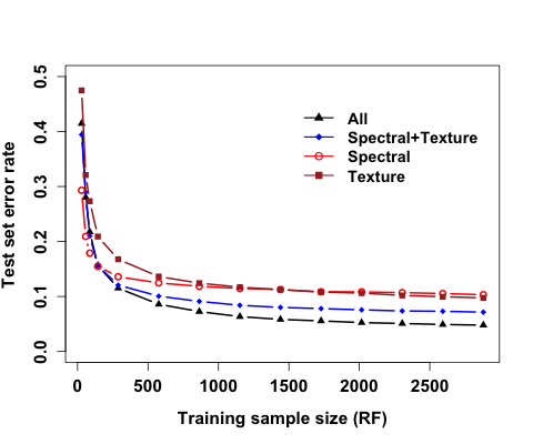
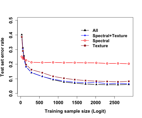
Figure 5: Error rates for spectral features, texture features, spectral and texture combined, and with additional location features when the sample size varies. The two panels correspond to RF and $L_{1}$ logistic regression, respectively. ‘Logit’ is short for logistic regression.

Figure 5 shows the error rates for varying sample sizes when using 4 different sets of features, including: 1) spectral features alone; 2) texture features alone; 3) combination of the two; 4) the combination with additional location features (latitude and longitude). In all 4 cases, there is an overall decreasing trend in the error rates when increasing the sample size. The two plots show very similar patterns except that the error rate curve with spectral features alone quickly levels off for $L_{1}$ logistic regression.

This implies that even if further enlarging the training sample, there would still be a gap between the empirical and the Bayes error when using only the spectral features (totally 6). Clearly a logistic regression model, as a linear model, would converge very quickly on 6 variables. Thus such a gap is likely caused by the fact that the richness of the logistic regression models (using only the 6 spectral features) is not sufficient to match the complexity of the problem thus a non-vanishing approximation error.

Figure 5 suggests that, in all cases, further increasing the sample size may not gain much in reducing the overall error. This is bacause the convergence error is close to 0 since the curves already level off. As many different algorithms have been tried [27], the approximation error should be very small for the best performing algorithm (see also the discussion on results by confusion matrix in Section 6.6). Thus it may be more worthwhile to explore the features dimension than the algorithms dimension. This is an insight we arrive at by exploring the sample and the algorithms dimensions. Later in Section 6.6, we will give clues on what kind of new features are likely worthwhile to further explore.

6.2 Error rates under label noise

As mentioned in Section 5.1, we will evaluate error rates under varying degrees of label noises. An $\epsilon$ proportion of the training sample is randomly selected, and then their labels are flipped uniformly at random to a different label. The resulting sample is a contaminated version of the original one. The classifier will then be trained on the contaminated sample, and predictive accuracy evaluated on the clean (uncontaminated) test sample.

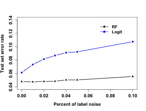
Figure 6: Error rates under label noises. The proportion of training sample with label noise is taken from {0.01, 0.02, 0.03, 0.04, 0.05, 0.10}.

Figure 6 shows error rates as $\epsilon$ varies over the set $\{0.01,0.02,0.03,0.04,0.05,0.10\}$. The error rate for $L_{1}$ logistic regression increases notably as $\epsilon$ increases from 0.01 to 0.10. However, the error curve for RF remains fairly flat. This indicates that RF is more resistant to label noise than $L_{1}$ logistic regression. The almost flat trend of the error curve for RF would allow us to confidently conclude that either the original label noise (extrapolated from the curve) is very small or its impact is negligible when using RF.

6.3 Marginal benefit of spectral, texture and location features

Many existing studies suggest that considering multiple features from different domains may be helpful to land classification [45, 44]. So it is natural to expect that combing the texture features and spectral features would do better than using either alone. As shown in Figure 5, this is the case when the sample size is not ‘small’. Here, by ‘small’ we mean a sample size less than about 20 instances per land-use type. Such a cutoff is consistent with recommendations made in [27]. This could be explained by the distance of separation.

Figure 7 shows the distance of separation for all pairs of land-use types (the distance of separation is only defined for a two-class classification problem in this work, and extension to multiple-class will be studied in our future work). It can be seen that for all pairs of land-use types, the distance of separation increases substantially when combining the spectral and texture features. Thus, as long as the training sample is large enough and the family of classifiers is rich enough, we will see reduced empirical error rates.

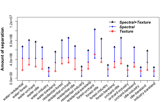
Figure 7: Distance of separation of all pairs of land types.

However, the improvement with RF when combining spectral and texture features (or adding spectral features in $L_{1}$ logistic regression when there are already texture features), which is about 2-3%, is far less than expected. In other words, the marginal benefits of spectral or texture features are small w.r.t. the other. This again could be understood from Figure 7 where the distance of separation between any pair is already big using either the spectral features or the texture features alone. A big distance of separation implies a small Bayes error. Thus, the room for improvement is small, and the marginal benefit of either the texture features or the spectral features w.r.t. the other is small.

Another observation from Figure 5 is that the spectral features and the texture features lead to similar empirical error rates (for RF only) when the sample size is not small. This can also be explained by Figure 7 where all the distances of separation for the spectral and texture features are large and of a similar magnitude thus the Bayes error for both cases would be close to 0. Regarding the Bayes error of this land classification problem with all features, we expect it be fairly close to 0 (the error rate when using RF is about 4.79%). The empirical error we get is a little upper-biased, due possibly to the discrepancy in class distribution between the test and the training sample according to discussions in Section 3. This is further confirmed by Figure 13.

In Figure 5, we also observe that adding location features (i.e., latitude and longitude) leads to noticeable reduction in the error rates when the sample size is large. In the case of RF, the error rate reduces by about 2%. This may be a little surprising, but could be understood by Theorem 4.2. A low ‘dependence’ between the location and other features can be seen clearly in Figure 8 (indicated by the bright colour in the first two rows and columns). Thus, by Theorem 4.2, we would expect an increased distance of separation when adding the location features thus a lower Bayes error. With a large sample size, this translates to a reduced error rate. In other words, the location features have a positive marginal benefit w.r.t. the spectral and texture features. Note that we cannot use Theorem 4.2 to explain the positive marginal benefits of either the spectral or the texture features w.r.t. the other, as clearly these features are highly correlated by Figure 8 (indicated by dark colour).

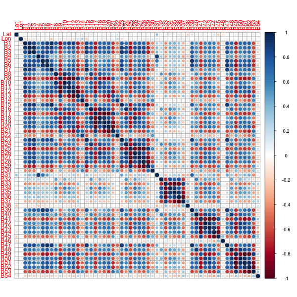
Figure 8: Heatmap of the covariance matrix.

6.4 Performance under small sample sizes

As mentioned before, it is often not feasible to obtain a large sample, especially for a new study. Here, we explore small training sample with sizes ranging from 28 to 140, or about 4 to 20 observations per land-use type. We observe that in such cases, combining spectral and texture features is no longer beneficial. Instead using spectral features alone actually outperforms the combination of both. This can be seen from Figure 9 which is a closeup-view of Figure 5. For such small sample sizes, combining the spectral and texture features would increase the data dimension to 54 (6 spectral features and 48 texture features) thus the curse of dimensionality [24] phenomenon occurs and the performance of the classifier deteriorates. This reaffirms that the usual recommendation [27] of having at least 20 observations per land-use type is reasonable.

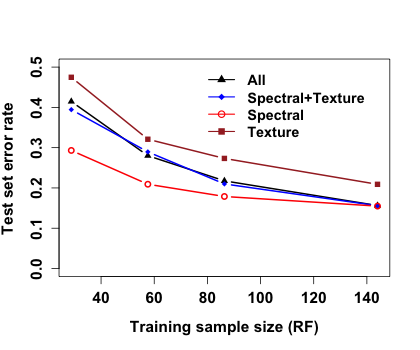
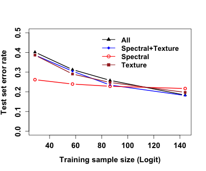
Figure 9: Error rates for spectral features, texture features, spectral and texture combined, and with additional location features under small sample sizes. The two panels correspond to RF and logistic regression, respectively.

Additionally, we observe that, when the sample is ‘small’, the spectral features are more ‘efficient’ than the texture features. This is again the result of sample size and model richness tradeoff as the number of spectral features and texture features are 6 and 48, respectively thus much smaller convergence error while not substantially higher approximation error when using spectral features alone. Also, Figure 7 shows that, in many cases (almost all but those involving the ‘Industry’ class), the spectral features have a larger distance of separation (thus smaller feature error). We view this as an implication of the strength of the spectral features.

6.5 Important features

Figure 5 and Figure 9 suggest that when the training sample is small, feature selection may be desirable during model fitting. Both RF and $L_{1}$ logistic regression have feature selection capability. In the following, we only report results obtained by RF as it has a built-in tool in producing feature importance.

Figure 10 shows the feature importance profile by RF. The top 10 most important features are B1-7, B31, B39, B14. Surprisingly, there is a major overlap with the spectral features B1-6. But this is consistent with our previous statements (c.f. Section 6.4) that the spectral features are ‘strong’ features. Additional important features are B7, B31, B39, B14, which—except B14 the correlation texture feature for TM band 1—are the mean of texture feature values for TM band 1, 4, and 5, respectively (the next three important features are B15, B47 and B23, which are the mean of texture features for TM band 2, 6 and 3, respectively). This is because the mean values carry a lot of information.

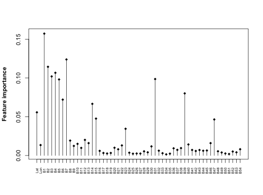
Figure 10: Variable importance produced by RF.

Additionally, ‘Latitude’ is an important feature (and ‘Longitude’, which is more important than many texture features). This makes sense, as there is a high correlation between neighboring pixels in the image, and the land-use information of an image pixel has a strong predictive ability about that of its neighbors.

6.6 Which land-use types are harder to classify?

As a matter of fact, the classification of different land-use types involves a varying level of difficulty. It will be helpful to figure out those land-use types that are harder than others, and a further study of which will likely reduce the overall error rate. The confusion matrix is an ideal tool for this purpose. We will use the confusion matrix produced by RF for the sake of convenience (logistic regression has comparable predictive accuracy as RF when using the texture features or all the features, but inferior with spectral features alone).

Table 4 shows the confusion matrices. There are three numbers in each cell, indicating results produced with all features, spectral features only, and texture features only, respectively. We have several observations

• Between many pairs of land-use types, there is a zero classification error. This can be explained by their large distance of separation as shown in Figure 7 and that the training sample size (which is 2880) is sufficiently large (error curves level off in Figure 5) thus small convergence errors. We hypothesize that the approximation error (not observable from experiments) resulting from using the RF classifiers is also ‘small’.

• The major misclassification occurs between two cases, ‘Forest’ vs Orchard’, and ‘Residential’ vs ‘Industry’. These two cases may be of a different nature though; see detailed discussions later.

• Overall, ‘Industry’ is a land-use type that is difficult to classify. It is often mis-classified as other types, or other types classified as ‘Industry’. This may be explained by the relatively smaller distance of separation between ‘Industry’ and other land-use types, as shown in Figure 7.

• Combining spectral and texture features helps the most in distinguishing ‘Forest’ vs ’Orchard’, and ‘Residential’ vs ‘Industry’. This is also true for varying sample sizes and more pronounced for larger sample sizes, according to Figure 11 and Figure 12. This later observation is expected as the convergence error would be smaller for larger sample sizes.

	Bareland	Forest	Idle	Industry	Orchard	Residential	Water
Bareland	42	0	0	2	0	0	0
	42/41	0/0	0/0	2/2	0/0	0/1	0/0
Forest	0	73	1	0	9	0	0
	0/0	63/69	3/0	0/0	16/13	0/0	1/1
Idle	0	1	44	0	0	0	0
	0/1	0/1	44/41	0/0	1/0	0/2	0/0
Industry	2	0	1	66	0	2	0
	2/3	0/0	1/2	65/64	0/0	3/2	0/0
Orchard	0	0	0	0	48	0	0
	0/0	2/0	0/2	0/0	46/45	0/0	0/1
Residential	0	0	0	1	0	89	1
	0/0	0/0	0/2	11/5	0/0	79/82	1/2
Water	0	0	0	0	0	0	41
	0/0	0/0	0/0	0/0	0/0	0/0	41/41

Table 4: Confusion matrix produced by RF. In each cell, there are three numbers for results using all features, spectral features or texture features alone, respectively.

Figure 7 shows a relatively small distance of separation for ‘Residential’ vs ‘Industry’. This implies that it may be more productive to add additional informative features to reduce the feature error. The later is consistent with our understanding—the difficulty in distinguishing ‘Residential’ vs ‘Industry’ lies in the fact that both land-use types are highly heterogeneous, and these two are similar in many aspects.

How to further reduce the error in ‘Residential’ vs ‘Industry’? One idea is to over-represent the ‘Industry’ class in the training sample as in [27, 16]. In the training sample, the land type ‘Industry’ already has 960 instances, much larger than other land types so it is already over-represented. To see the effect of over-representation, as we do not have a larger sample, we downsample the ‘Industry’ class and use the trend to infer the effect of overrepresentation.

Figure 13 shows the error rate and the number of misclassified test instances involving ‘Industry’ (i.e., all instances with a land-use type ‘Industry’ or been classified as ‘Industry’) with different down-sampling ratios for the ‘Industry’ land-use type. It can be seen that the smallest error rate for both are achieved at roughly a sampling ratio of 0.6 (to match the class distribution in the test sample, the sampling ratio should be around 0.4). So overrepresentation helps a little bit, but further overrepresentation will not help. This is likely due to the fact that further increasing the sampling ratio would cause more discrepancy between the training and the test sample thus a larger error rate. As the convergence error is already small (level-off on various error curves) and the approximation error with RF is hypothesized to be small, a possible future direction is to try reducing the feature error, i.e., look for features that would better distinguish ‘Residential’ vs ‘Industry’.

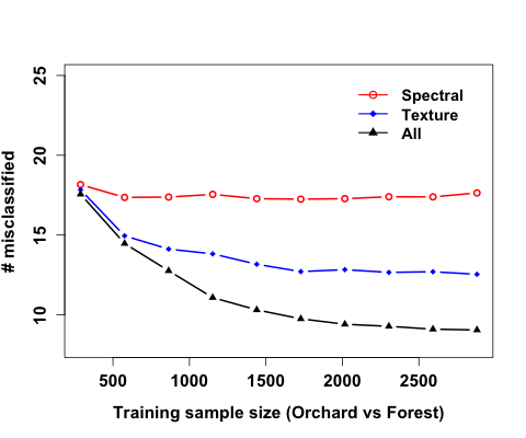
Figure 11: Number of misclassified instances in distinguishing ‘Orchard’ from ‘Forest’ as sample size increases. The three curve correspond to using spectral feature, texture features, and the two combined, respectively.

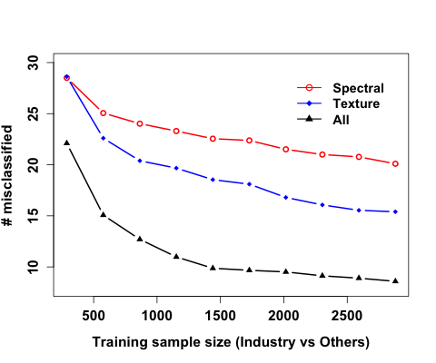
Figure 12: Number of misclassified instances in distinguishing ‘Industry’ from other land-use types as sample size increases. The three curve correspond to using spectral feature, texture features, and the two combined, respectively.

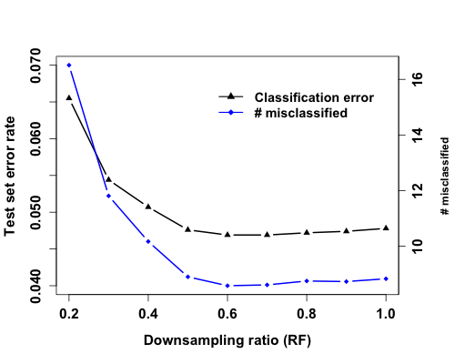
Figure 13: Error rate and the number of misclassified instances involving ‘Industry’ when downsampling the ‘Industry’ class in the training sample.

7 Conclusions

In this paper, we propose a structured approach for the analysis of a land-use classification study. Under our model for structured analysis, we view the outputs (e.g., error), one dimension of a study, as a result of the interplay of other three dimensions, including feature, sample, and algorithms. Moreover, the land-use classification error can be further decomposed into error components according to these three dimensions. Such a structural decomposition of entities involved in land-use classification would help us better understand the nature of a land classification study, and potentially allow better trace of the merits or difficulty of a study to a more concrete source entity, or a more refined characterization of the difficulty of the problem. The analysis of a remote sensing image about a study site in Guangzhou, China, is used to demonstrate how a structured analysis could be carried out. We are able to identify a few possible directions for future studies that would potentially further reduce the land-use classification error; such information are typically beyond a usual land-use classification study. We expect the structured analysis as we have proposed will inform practices in the analysis of remote sensing images, and help advance the state-of-the-art of study on the land-use classification problem.

8 Proof of Theorem 4.2

Proof.

The proof uses perturbation analysis [25, 41, 42], and follows a similar line of arguments as [42].

To simplify notations, write

$$\bm{A}=\left[\begin{array}[]{cc}\bm{A}_{11}&\bm{0}\\ \bm{0}&\bm{A}_{22}\\ \end{array}\right]$$

and

$$\bm{E}=\left[\begin{array}[]{cc}\bm{0}&\bm{E}_{12}\\ \bm{E}_{12}^{T}&\bm{0}\\ \end{array}\right]$$

where $\bm{0}$’s denote null matrices with appropriate dimensions and $\bm{E}_{12}=\bm{A}_{12}$. Thus $\bm{\Sigma}=\bm{A}+\bm{E}$. To facilitate the calculation of $\bm{u}_{\bm{\mathcal{F}}}^{T}\bm{\Sigma}^{-1}\bm{u}_{\bm{\mathcal{F}}}$, we will first derive a Taylor’s series expansion result. Since

$$||\bm{E}||_{F}^{2}=2||\bm{E}_{12}||_{F}^{2}=2||\bm{A}_{12}||_{F}^{2}$$ (7)

and $||\bm{A}^{-1}\bm{E}||_{F}\leq||\bm{A}^{-1}||_{F}||\bm{E}||_{F}\leq\sqrt{\mbox{rank}(\bm{A}^{-1})}||\bm{A}^{-1}||_{2}||\bm{E}||_{F}$ (by the sub-multiplicative property of the Frobenius norm [18] and the boundedness of the eigenvalues of $\bm{A}^{-1}$), the following Taylor’s series expansion is valid

$$(\bm{I}+\bm{A}^{-1}\bm{E})^{-1}=\bm{I}-\bm{A}^{-1}\bm{E}+O[(\bm{A}^{-1}\bm{E})^{2}],$$ (8)

where $O$ in the above is the big-O notation. It follows that

$$\bm{u}_{\bm{\mathcal{F}}}^{T}\bm{\Sigma}^{-1}\bm{u}_{\bm{\mathcal{F}}} = [\bm{u}_{1},\bm{u}_{2}]^{T}(\bm{A}+\bm{E})^{-1}[\bm{u}_{1},\bm{u}_{2}]$$ (9)

$$= [\bm{u}_{1},\bm{u}_{2}]^{T}(I-\bm{A}^{-1}\bm{E}+O[(\bm{A}^{-1}\bm{E})^{2}])\bm{A}^{-1}[\bm{u}_{1},\bm{u}_{2}]$$

$$= [\bm{u}_{1},\bm{u}_{2}]^{T}(\bm{A}^{-1}-\bm{A}^{-1}\bm{E}\bm{A}^{-1}+O[(\bm{A}^{-1}\bm{E})^{2}]\bm{A}^{-1})[\bm{u}_{1},\bm{u}_{2}]$$

$$= [\bm{u}_{1},\bm{u}_{2}]^{T}\bm{A}^{-1}[\bm{u}_{1},\bm{u}_{2}]-[\bm{u}_{1},\bm{u}_{2}]^{T}\bm{A}^{-1}\bm{E}\bm{A}^{-1}[\bm{u}_{1},\bm{u}_{2}]$$

$$+[\bm{u}_{1},\bm{u}_{2}]^{T}O[(\bm{A}^{-1}\bm{E})^{2}]\bm{A}^{-1}[\bm{u}_{1},\bm{u}_{2}]$$

$$= \mathcal{S}_{1}+\mathcal{S}_{2}+\mathcal{S}_{3}.$$

$\mathcal{S}_{1}$ can be calculated as

$$\mathcal{S}_{1}=[\bm{u}_{1},\bm{u}_{2}]^{T}\left[\begin{array}[]{cc}\bm{A}_{11}&\bm{0}\\ \bm{0}&\bm{A}_{22}\\ \end{array}\right]^{-1}[\bm{u}_{1},\bm{u}_{2}]=\bm{u}_{1}^{T}\bm{A}_{11}^{-1}\bm{u}_{1}+\bm{u}_{2}^{T}\bm{A}_{22}^{-1}\bm{u}_{2}.$$ (10)

We have

$$||\mathcal{S}_{2}||_{F}\leq||\bm{u}||_{F}^{2}.||\bm{A}^{-1}||_{F}^{2}||\bm{E}||_{F}\leq C^{2}||\bm{A}^{-1}||_{F}^{2}||\bm{E}||_{F}=o(1)$$ (11)

since $||\bm{A}||_{F}\leq\sqrt{\mbox{rank}(\bm{A})}||\bm{A}||_{2}$ and $||\bm{A}^{-1}||_{F}\leq\sqrt{\mbox{rank}(\bm{A}^{-1})}||\bm{A}^{-1}||_{2}$ (where $||.||_{2}$ denote the 2-norm of a matrix) and by the boundedness of the eigenvalues of $\bm{A}$ and $\bm{A}^{-1}$. Similarly, we have

$$||\mathcal{S}_{3}||_{F}\leq||\bm{u}||_{F}^{2}||\bm{A}^{-1}||_{F}^{3}||\bm{E}||_{F}^{2}=o(1).$$ (12)

Combining equations (10), (11) and (12) yields

$$\bm{u}_{\bm{\mathcal{F}}}^{T}\bm{\Sigma}^{-1}\bm{u}_{\bm{\mathcal{F}}}=\bm{u}_{1}^{T}\bm{A}_{11}^{-1}\bm{u}_{1}+\bm{u}_{2}^{T}\bm{A}_{22}^{-1}\bm{u}_{2}+o(1).$$ (13)

Since both $\bm{u}_{1}^{T}\bm{A}_{11}^{-1}\bm{u}_{1}$ and $\bm{u}_{2}^{T}\bm{A}_{22}^{-1}\bm{u}_{2}$ are nonnegative, the claim of the theorem has been proved. ∎

References

- [1] T. W. Anderson. An Introduction to Multivariate Statistical Analysis. John Wiley & Sons, 1958.
- [2] D. A. Belsley, E. Kuh, and R. E. Welsch. Regression diagnostics : identifying influential data and sources of collinearity. Wiley., New York, NY, USA, 1980.
- [3] P. J. Bickel and E. Levina. Regularized estimation of large covariance matrices. The Annals of Statistics, 36(1):199–227, 2008.
- [4] L. Breiman. Random Forests. Machine Learning, 45(1):5–32, 2001.
- [5] L. Breiman, J. Friedman, C. J. Stone, and R. A. Olshen. Classification and Regression Trees. Chapman and Hall/CRC, 1984.
- [6] R. Caruana, N. Karampatziakis, and A. Yessenalina. An empirical evaluation of supervised learning in high dimensions. In Proceedings of the Twenty-Fifth International Conference on Machine Learning (ICML), pages 96–103, 2008.
- [7] R. Caruana and A. Niculescu-Mizil. An empirical comparison of supervised learning algorithms. In Proceedings of the 23rd International Conference on Machine Learning (ICML), 2006.
- [8] S. Chen and D. L. Donoho. Basis pursuit. In 28th Asilomar Conference on Signals, Systems and Computers, pages 41–44, 1994.
- [9] R. D. Cook and S. Weisberg. Diagnostics for heteroscedasticity in regression. Biometrika, 70(1):1–10, 1983.
- [10] C. Cortes and V. N. Vapnik. Support-vector networks. Machine Learning, 20(3):273–297, 1995.
- [11] D. L. Donoho and I. M. Johnstone. Ideal spatial adaption by wavelet shrinkage. Biometrika, 81:425–455, 1994.
- [12] R. O. Duda and P. E. Hart. Pattern Classification and Scene Analysis. Wiley, 1973.
- [13] F. L. Fan, Y. P. Wang, M. H. Qiu, and Z. S. Wang. Evaluating the temporal and spatial urban expansion patterns of Guangzhou from 1979 to 2003 by remote sensing and GIS methods. International Journal of Geographical Information Science, 23(11):1371–1388, 2009.
- [14] F. L. Fan, Q. H. Weng, and Y. P. Wang. Land use and land cover change in Guangzhou, China, from 1998 to 2003, based on Landsat TM/ETM+ imagery. Sensors, 7(7):1323–1342, 2007.
- [15] J. Fan, Y. Liao, and H. Liu. An overview of the estimation of large covariance and precision matrices. The Econometrics Journal, 19(1):C1–C32, 2016.
- [16] Y. Freund and R. Schapire. Experiments with a new boosting algorithm. In International Conference on Machine Learning (ICML), 1996.
- [17] J. Friedman, T. Hastie, and R. Tibshirani. Regulzrization paths for generalized linear models via coordinate descent. Journal of Statistical Software, 33(1):1–22, 2010.
- [18] G. H. Golub and C. F. Van Loan. Matrix Computations. Johns Hopkins, 1989.
- [19] P. Gong and P. J. Howarth. Land-use classification of SPOT HRV data using a cover-frequency method. International Journal of Remote Sensing, 24(21):4137–4160, 2003.
- [20] P. Gong, D. Marceau, and P. J. Howarth. A comparison of spatial feature extraction algorithms for land-use classification with SPOT HRV data. Remote Sensing of Environment, 40:137–151, 1992.
- [21] P. Gong, J. Wang, L. Yu, Y. Zhao, Y. Zhao, L. Liang, Z. Niu, X. Huang, H. Fu, S. Liu, C. Li, X. Li, W. Fu, C. Liu, Y. Xu, X. Wang, Q. Cheng, L. Hu, W. Yao, H. Zhang, P. Zhu, Z. Zhao, H. Zhang, Y. Zheng, Luyan Ji, Y. Zhang, H. Cheng, A. Yang, J. Guo, L. Yu, L. Wang, X. Liu, T. Shi, M. Zhu, Y. Chen, G. Yang, P. Tang, B. Xu, C. Giri, N. Clinton, Z. Zhu, J. Chen, and J. Chen. Finer resolution observation and monitoring of global land cover: first mapping results with Landsat TM and ETM+ data. International Journal of Remote Sensing, 34(7):2607–2654, 2013.
- [22] I. Guyon and A. Elisseeff. An introduction to variable and feature selection. Journal of Machine Learning Research, 3:1157–1182, 2003.
- [23] F. R. Hampel. The influence curve and its role in robust estimation. Journal of the American Statistical Association, 69(346):383–393, 1974.
- [24] T. Hastie, R. Tibshirani, and J. Friedman. The Elements of Statistical Learning: Data Mining, Inference, and Prediction. Springer, 2001.
- [25] L. Huang, D. Yan, M. I. Jordan, and N. Taft. Spectral clustering with perturbed data. In Advances in Neural Information Processing Systems (NIPS), volume 21, 2009.
- [26] G. S. Kimeldorf and G. Wahba. Correspondence between Bayesian estimation on stochastic processes and smoothing by splines. Annals of Mathematical Statistics, 41:495–502, 1970.
- [27] C. Li, J. Wang, L. Wang, L. Hu, and P. Gong. Comparison of classification algorithms and training sample sizes in urban land classification with Landsat thematic mapper imagery. Remote Sensing, 6(2):964–983, 2014.
- [28] H. Liu and H. Motoda. Feature Selection for Knowledge Discovery and Data Mining. Springer, 1998.
- [29] G. J. McLachlan and D. Peel. Finite Mixture Models. Wiley, 2000.
- [30] X. Nguyen, L. Huang, and A. D. Joseph. Support vector machines, data reduction and approximate kernel matrices. In Proceedings of European Conference on Machine Learning (ECML), 2008.
- [31] M. Park and T. Hastie. L1-regularization path algorithm for generalized linear models. Journal of the Royal Statistical Society (B), 69(4):659–677, 2007.
- [32] J. A. Rice. Mathematical Statistics and Data Analysis. Duxbury Press, 1995.
- [33] K. C. Seto, C. Woodcock, C. Song, X. Huang, J. Lu, and R. Kaufmann. Monitoring land-use change in the Pearl River Delta using Landsat TM. International Journal of Remote Sensing, 10:1985–2004, 2002.
- [34] J. Tang, S. Alelyani, and H. Liu. Feature selection for classification: A review. In C. C. Aggarwal, editor, Data Classification: Algorithms and Applications. Chapman and Hall/CRC, 2014.
- [35] R. Tibshirani. Regression shrinkage and selection via the lasso. Journal of Royal Statistics Society (Series B), 58(1):267–288, 1996.
- [36] A. N. Tikhonov. On solving ill-posed problem and method of regularization. Doklady Akademii Nauk USSR, 153:501–504, 1963.
- [37] K. M. Ting. Encyclopedia of machine learning. Springer, 2011.
- [38] J. W. Tukey. A survey of sampling from contaminated distributions. In I. Olkin, editor, Contributions to Probability and Statistics, pages 448–485. Standford University Press, 1960.
- [39] G. Wahba. Spline Models for Observational Data. SIAM, Philadelphia, PA, 1990.
- [40] D. Yan, P. Gong, A. Chen, and L. Zhong. Classification under data contamination with application to remote sensing image mis-registration. arXiv:1101.3594, 2011.
- [41] D. Yan, L. Huang, and M. I. Jordan. Fast approximate spectral clustering. In Proceedings of the 15th ACM SIGKDD, pages 907–916, 2009.
- [42] D. Yan, P. Wang, B. S. Knudsen, M. Linden, and T. W. Randolph. Statistical methods for tissue microarray images–algorithmic scoring and co-training. The Annals of Applied Statistics, 6(3):1280–1305, 2012.
- [43] L. Yu, L. Liang, J. Wang, Y. Zhao, Q. Cheng, L. Hu, S. Liu, L. Yu, X. Wang, P. Zhu, X. Li, Y. Xu, C. Li, W. Fu, X. Li, W. Li, C. Liu, N. Cong, H. Zhang, F. Sun, X. Bi, Q. Xin, D. Li, D. Yan, Z. Zhu, M. Goodchild, and P. Gong. Meta-discoveries from a synthesis of satellite-based land-cover mapping research. International Journal of Remote Sensing, 35(13):4573–4588, 2014.
- [44] L. Zhang, Q. Zhang, B. Du, X. Huang, Y. Y. Tang, and D. Tao. Simultaneous spectral-spatial feature selection and extraction for hyperspectral images. IEEE Transactions on Cybernetics, 48(1):16–28, 2018.
- [45] L. Zhang, Q. Zhang, L. Zhang, D. Tao, X. Huang, and B. Du. Ensemble manifold regularized sparse low-rank approximation for multiview feature embedding. Pattern Recognition, 48(10):3102–3112, 2015.
- [46] X. Zhu and X. Wu. Class noise vs. attribute noise: a quantitative study of their impacts. Artificial Intelligence Review, 22(3):177–210, 2004.