3.5cm2.5cm1cm1cm 2021

Selected Chapters on
Active Galactic Nuclei as Relativistic Systems

Astrophysical black holes in nuclei of galaxies are of indisputable relevance to the current research. These extreme objects are of immense interest to pure relativists as well as observational astronomers. This diversification is reflected in varied approaches that people adopt to the problem. Mathematically minded theorists take more interest in analytical solutions to Einstein’s equations and idealized systems where the role of strong gravity can be exposed. Observers want to actually see the gas flows swirling in the form of an accretion disk or a torus. Astronomers often invoke disk-type accretion to explain spectral features observed in galactic nuclei, although the detailed physics of accretion flows still remains incomplete.  
Despite that the processes in strong gravity govern only the innermost regions of accretion disks, their role is quickly diminished with the distance from the source. Non-gravitational physics plays a crucial role and it often dominates the acceleration and emission processes. In order to see where the limitations of our models are, it is useful to discuss simplified and general analytical models along with particular astronomical objects.  
These lecture notes present an overview of selected aspects of physical processes occurring in the inner regions of Active Galactic Nuclei (AGN). Observational evidence strongly suggests that strong gravitational fields play a significant role in governing the energy output of AGN and their influence on the surrounding medium due to the presence of a supermassive black hole (SMBH) or a system of SMBHs undergoing a merger. We begin by an account of observational properties of AGN, their basic structural components and unification scenarios, and the arguments for the presence of SMBHs in their cores. Subsequently, in more detail, we discuss selected phenomena that are related to black-hole accretion and relevant for the emerging radiation signal and the acceleration of matter in AGN cores.  
In order to reduce an unnecessary overlap with numerous reviews and textbook chapters on the similar subject, we focus on just a few topics, such as the launching scenarios of nuclear outflows and jets that start and pre-collimate in the immediate vicinity of black holes, at distance of only a few gravitational radii, and then can reach spectacular length-scales of $\sim$Mpc, extending far beyond the host galaxy. We also discuss the interaction between magnetic and gravitational fields in the strong-gravity regime of General Relativity. Some more recent aspects of the AGN unification scheme are included and quite a large number of references are provided to relevant papers and textbooks at the end of the volume. The interested reader is invited to consult the original works, which can provide an exciting context to the lively research on Active Galactic Nuclei.  

Cover photo: Cygnus A active galaxy is shown on a collage across the electromagnetic spectrum: the X-ray signal (blue) from the Chandra Observatory have been superimposed over the radio emission (red), which extends to nearly 300,000 light-years. Jets of relativistic particles emanate to either side from the galaxy’s central supermassive black hole and mark the hot spots at both ends at the impact onto the surrounding material. Optical data (yellow) from Hubble Space Telescope and the Digital Sky Survey complete the multi-wavelength view.

Keywords: galaxies: active; black holes: supermassive; relativistic physics

1 Defining properties of Active Galactic Nuclei

“Do not undertake a scientific career in quest of fame or money. There are easier and better ways to reach them. Undertake it only if nothing else will satisfy you; for nothing else is probably what you will receive. Your reward will be the widening of the horizon as you climb. And if you achieve that reward you will ask no other."

— Cecilia Payne-Gaposchkin

Active galactic nuclei (AGN) are compact cores of a special category of galaxies that are characterized by high luminosity of non-stellar origin. They are distinguished also by the spectral energy distribution (SED) of the emerging radiation which spans a wide range of electromagnetic spectrum – from low-frequency radio waves across millimeter, infrared, and optical light, and further up to X-rays and high-energy gamma-rays. Most AGN are characterized by a strong emission in UV, known as the Big Blue Bump, and emission in X-rays much exceeding the typical X-ray luminosity of normal, non-active, galaxies. Some AGN exhibit powerful jets, collimated to a very narrow cone and moving by strongly relativistic velocities up to the intergalactic space. There is a plenty of different observational evidence of the nuclear activity in various sources that lead to classification of several different kinds of AGN (occasionally referred to as an AGN zoology). This various appearance strongly depends on the orientation of the AGN with respect to the observer (as we will more discuss in sect. 1.3). Our aim is not to fully describe all observed kinds of AGN, but rather introduce the main characteristic features.

Based on a broad spectrum of observational evidence it has been generally accepted that the common denominator for AGN activity is the presence of at least one supermassive black hole (SMBH) that accretes the surrounding matter. A variety of physical processes must operate and a wide range of physical conditions must occur, namely, density, pressure and temperature of the diluted environment, and intensity of the magnetic field and of the radiation field pervading the SMBH neighborhood. Accretion rate and the spin of the black hole appear to be the main parameters influencing the intrinsic properties of active nuclei. Whereas numerical simulations are necessary to model the evolution of the system, it turns out that idealized scenarios can reflect underlying physical mechanisms in their mutual interplay. We will attempt to supplement the vast literature that deals with the subject of AGN by the context of simplified toy-model approaches, where the number of degrees of freedom are reduced and only selected ingredients are taken into account.

Let us mention a subtle mystery that governs seemingly different and unrelated objects: the mass scaling and the corresponding length scales. An appropriate change of the scale by many orders of magnitude can bring us from one type of object to another, from SMBH in the cores of galaxies to their bulges and even beyond. This fact has been extensively investigated in the context of feedback mechanisms and even the impact on the large-scale structure of the Universe.

We will summarize arguments for the presence of such a giant black hole in AGN. The multiple convincing evidence has also been found in our own Galaxy. Unlike the cores of active galaxies, the $10^{6}$ solar mass black hole in the center of the Milky Way (Sagittarius A*) is, however, currently inactive; we will discuss this in section 1.5. In the following chapters, we will review the main radiation processes relevant for black-hole accretion (Chapt. 2) and jet-launching mechanisms (Chapt. 3). Finally, in Chapter 4, we will compare accretion on SMBH in AGN with the case of stellar-mass black holes in X-ray binaries. Readers are referred to numerous monographs and review articles [e.g., 365, 505, 586, 482] for further information about physics, observational properties and rich phenomenology of different kinds of AGN. A very recent exposition can be found in [513]. The importance of coevolution of SMBHs and their host galaxies, processes of SMBH growth and the resulting relation between the black hole mass and the bulge mass in AGN have been reviewed by Kormendy and Ho, [358].

1.1 AGN across wavelengths

The subject of AGN has grown enormously over recent three decades of intense investigation. Nowadays, it is an arena of a far too vast and interconnected observational and theoretical research to be covered in a single review. Even if we concentrate our attention on a restricted volume of the inner regions near SMBH, we have to omit many topics, including those ones that are of immense importance. We will attempt to formulate a compromise and provide a very limited introductory overview supplemented by several less-discussed aspects of current interest.

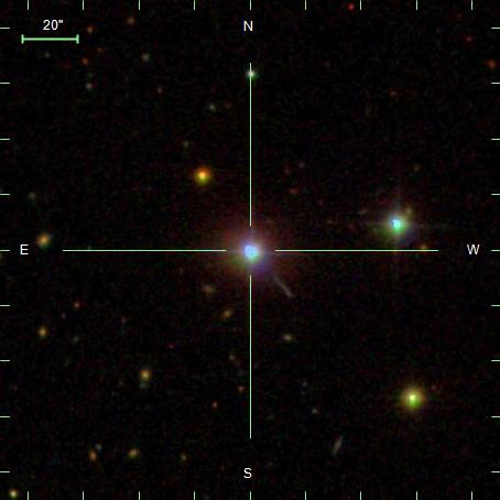
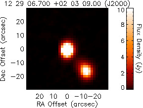
Figure 1: Left panel: Optical image of quasar 3C 273 adopted from SDSS optical survey [619]. Right panel: The radio counterpart of 3C 273 at the frequency of $1.4\,{\rm GHz}$. Figure from the FIRST survey [50].

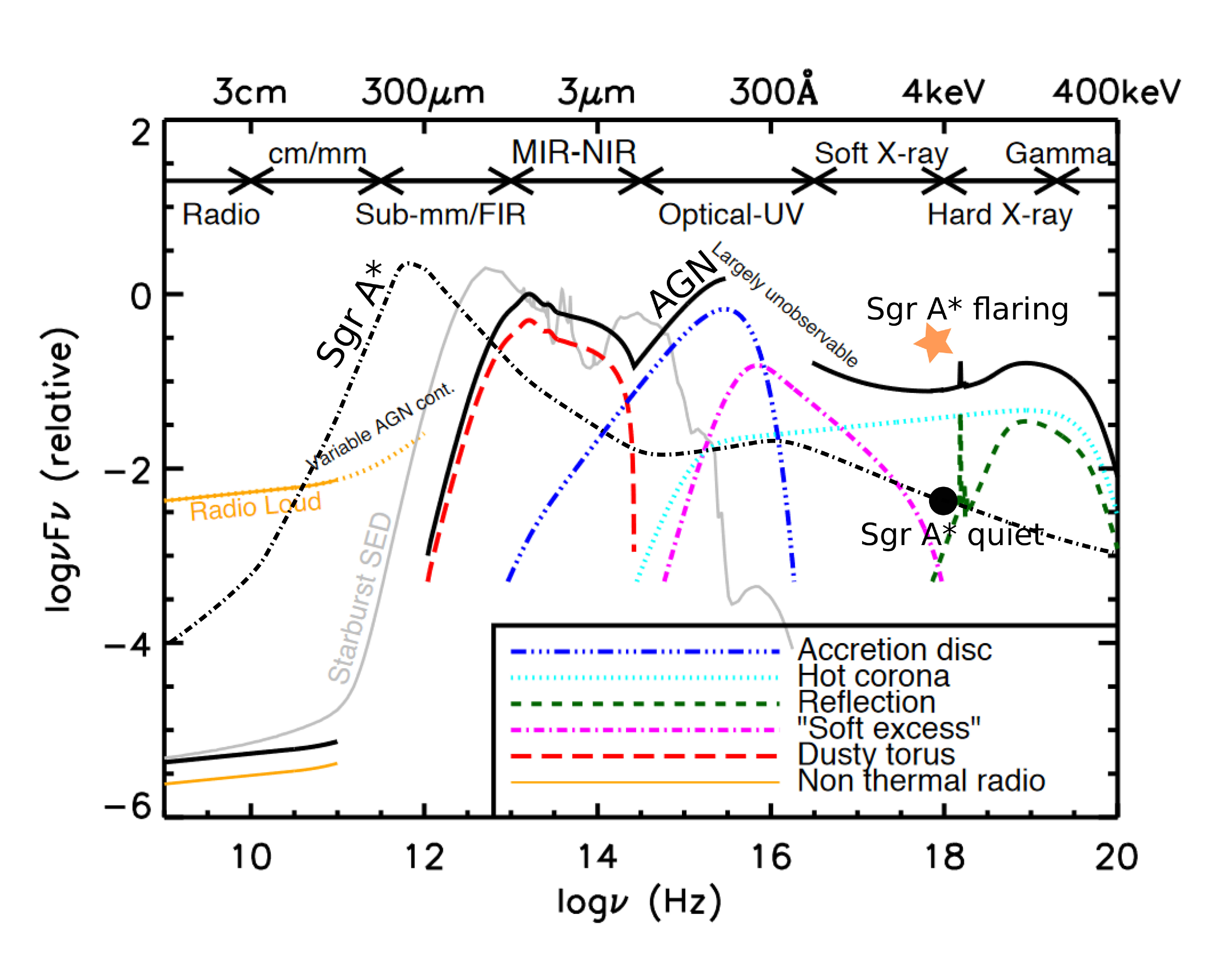
Figure 2: An illustrative view of the AGN spectral energy distribution (SED) based on the actual observational data of radio-quiet AGN [see references 211, 567, for more details]. The total AGN SED is depicted with a solid black line, while individual components (accretion disc, hot corona, reflection component, soft excess, dusty torus, and non-thermal radio component) are coloured. Towards sub-mm/FIR and radio domains, the non-thermal radio component depends on the jet activity (radio-loud vs. radio-quiet). For comparison, the SED of an extremely low-luminous AGN, represented by Sgr A*, is shown using a dot-dashed line. Sgr A* exhibits flares in the NIR/X-ray domains, which can increase the X-ray flux density by as much as several orders of magnitude. The solid grey line depicts the SED of a starburst galaxy, which peaks in the sub-mm/FIR domain [based on the SED of M82 adopted from the GRASIL library; 609]. The image was adopted from Harrison, [282] and modified to add the SED of Sgr A* according to Yuan and Narayan, [694].

Active galaxies differ from normal, inactive galaxies, such as our Milky Way, by significantly broader wavelength range of their electromagnetic spectrum, which can extend over the entire observable interval from radio wavelengths, through infrared, optical, UV, X-ray, up to gamma-ray wavelengths. Each wavelength puts a different piece into the mosaic. An example of an AGN is quasar 3C 273, whose image in optical and radio is shown in Fig. 1. While the optical image reveals bright emission from a point-like source (nucleus of the galaxy), the radio image reveals two spatially separated knots of the relativistic jet. However, the jet as a thin faint line can also be identified in the optical image, which is due to the broad-band synchrotron emission that can also extend from the radio to the optical domain. Multi-frequency observations are therefore necessary to fully understand the AGN structure and physics.

The SED of normal galaxies can be understood as the superposition of thermal spectra produced by stars of different surface temperature. Since the range of the stellar temperature is rather narrow, $T_{\rm eff}\gtrsim 3000\,{\rm K}$ and $T_{\rm eff}\lesssim 40\,000\,{\rm K}$, most of the bolometric luminosity of normal galaxies is emitted in the infrared, optical, and ultraviolet parts of the electromagnetic spectrum. AGN therefore require a different mechanism from the stellar thermal emission to explain their prominent radio, X-ray, and even gamma-ray emission. Furthermore, the enormous radiation output of AGN cannot often be detected directly; instead it is obscured by a lot of gas and dust that absorbs, modifies and reemits much of the characteristic observational signatures [289]. This reprocessing challenges observational methods to uncover the complete population and understand the evolution of SMBHs.

Within a limited energy range, the AGN SED can often be described as a power-law function,

$$L_{\nu}\propto\nu^{-\alpha},$$ (1)

where $\alpha$ is the spectral index. A schematic view of an AGN SED is shown in Fig. 2. Different physical components and mechanisms contribute to the SED and produce a more complicated spectrum, namely, a broken power-law with multiple values of the spectral index, or even a superposition with additional components and cut-off at a certain maximum energy. Thermal emission from the accretion disk, non-thermal emission from the hot corona, X-ray reflection, and reprocessed emission by the dusty torus, they all contribute to the SED. When the jet is present, the AGN SED extends to radio and gamma-rays and the jet contribution can even dominate the signal when pointing along the line of sight towards us (the case of so-called blazars). The AGN SED often peaks in the ultraviolet domain due to the multi-temperature thermal emission of an accretion disc, which is referred to as the big blue bump. In contrast, the spectrum of starburst galaxies (shown by a grey curve in Fig. 2) is limited mainly to the infrared and optical frequency bands, and peaks in the sub-mm/FIR domain. For comparison, in Fig. 2, we also show the SED of Sgr A*, the compact radio source in the center of the Milky Way. Sgr A* is a typical representative of extremely low-luminous galactic nuclei that accrete several orders of magnitude below the Eddington limit, see Eq. (22) for the definition. Low-luminous, quiescent galaxies are typically powered by optically thin and geometrically thick hot accretion flows [694] that are in contrast to optically thick and geometrically thin accretion discs that are present for highly-accreting AGN. The result is that for Sgr A*, the peak of its SED shifts towards longer wavelengths to the sub-mm/mm domain. In comparison with the thermal big blue bump, the sub-mm/mm peak arises due to the synchrotron emission of thermalized electrons of the magnetized hot flow.

Radio band

The radio band was the first band to discover AGN and quasars. The normal stars are very weak in radio band. Thus, the discoveries of optical point sources that have also strong radio emission led to the first identification of quasars. The quasar discovery was made by Schmidt, [585] who noticed a very large redshift ($z=0.158$) of emission lines in a star-like source from the 3C (The Cambridge 178 MHz radio survey) sample [201].

The AGN radio luminosity can enormously span the range over several orders of magnitude, and therefore, AGN are distinguished into radio-loud vs. radio-quiet sources. The majority of AGN are radio-quiet, while only about 10$\%$ are radio-loud [339, 40]. The reason for this dichotomy is the presence or absence of the strong relativistic jet launched by the SMBH. However, the radio-loud/quiet distinction and the reason behind it is not yet a settled problem. Different ideas were proposed to explain this dichotomy, including the spin paradigm [455, 606], observational selection effects [677, 133] or evolution of the spectral states [349, 630]. In the study of radio dichotomy, it is also important whether the total radio luminosity or only the core radio luminosity is taken into account [101]. This distinction is obviously possible only for local AGN but not for unresolved distant quasars.

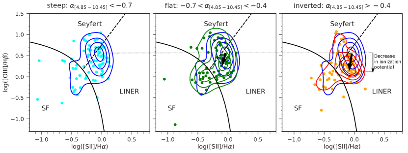
Figure 3: Distribution of sources with different radio spectral index in the narrow emission-line diagnostic diagram, also known as the Baldwin–Phillips–Terlevich (BPT) plot [39], where three spectral classes of galaxies are denoted: star-forming (SF), Seyfert, and LINER. From the left to the right, we see that steep sources have a tendency to group towards the Seyfert sources, i.e. a higher ionization potential, while inverted sources peak in the LINER region, i.e. towards a lower ionization potential. Figure adopted from Zajaček et al., 2020d [705]; see also Zajaček et al., 2019a [701] for a detailed analysis and a discussion.

The radio luminosity, spectrum and morphological classification depends on how bright the jet core is versus extended radio lobes created by the jet dissipation into the intergalactic matter. The original morphological classification by Fanaroff and Riley, [224] distinguishes between the radio-core (FR type I) and radio-lobes (FR type II) dominated sources. Later on, radio point sources were categorized as FR type 0. The radio spectral slope differs accordingly. The core-dominated spectra are typically radio-flat with $\alpha=0\pm 0.5$, while the radio lobe-dominated spectra are steep with $\alpha<-0.5$. A special class of inverted radio spectra was established for indices $\alpha>0.5$. Many more classes were introduced based on the radio spectral slope, e.g., Compact Steep Sources [225], Giga-Hertz Peak Sources [498], etc. The spectral index distribution is also correlated with the optical properties of host galaxies, specifically their ionizing potential traced by narrow emission-line ratios. In particular low-ionization narrow emission region (LINER) sources have a tendency for a flatter spectral index and a lower ionization potential expressed by the narrow emission-line ratio [OIII]/H$\beta$, while Seyfert sources have a steeper spectral index and a larger ionization potential, see Fig. 3 for the graphical representation in the optical diagnostic diagram and Zajaček et al., 2019a [701] for a detailed analysis. This distinction could be related to the duty cycle of the sources [160, 633], with Seyfert galaxies being active long enough to develop radio lobes, while LINER sources lack large radio lobes due to their old age or because of just recently restarted activity. In both cases, a compact self-absorbed radio core with a compact jet would dominate the total radio output, which would result in a flat or a potentially inverted radio spectral index due to the self absorption of the synchrotron emission.

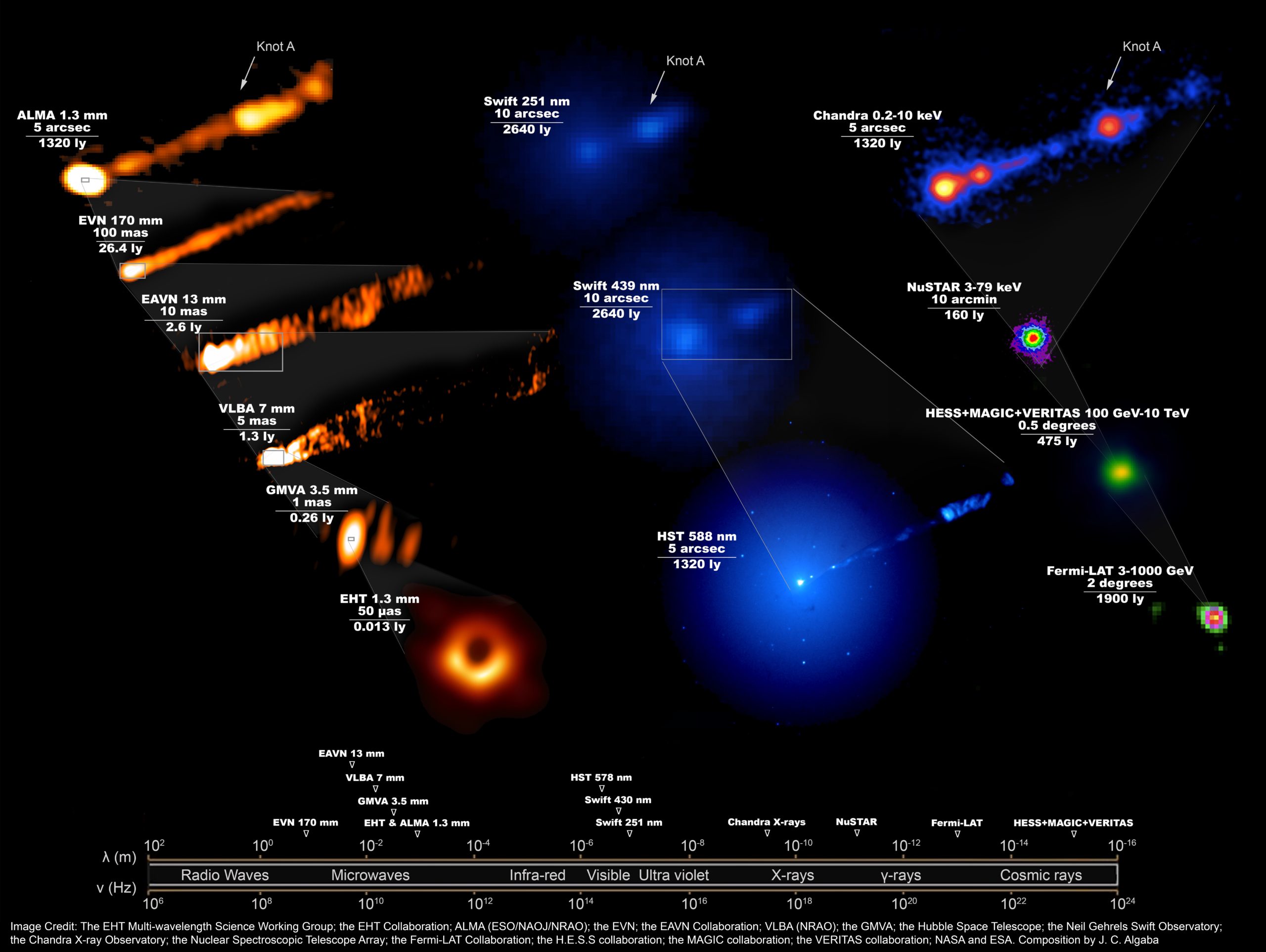
Figure 4: A collage of multi-wavelength images during the 2017 observing campaign of M87. 19 different instruments on the ground and in space had to be used to obtain the presented images. In the upper left corner, the ALMA image at 1.3 mm (orange) shows a large-scale jet structure, with a clear core region and knot A. This is comparable in projected scale to the optical HST image in the center as well as to the X-ray Chandra image in the upper right corner. Image credits: The EHT Multi-wavelength science working group; the EHT Collaboration; ALMA (ESO/NAOJ/NRAO); the EVN; the EAVN Collaboration; VLBA (NRAO); the GMVA; the Hubble Space Telescope; the Neil Gehrels Swift Observatory; the Chandra X-ray Observatory; the Nuclear Spectroscopic Telescope Array; the Fermi-LAT collaboration; the H.E.S.S. collaboration; the MAGIC collaboration; the VERITAS collaboration; NASA and ESA. The multi-wavelength composition by J. C. Algaba. (Based on the M87 multi-wavelength analysis by EHT MWL Science Working Group et al., [204].)

The high-resolution radio observations using very-long-baseline interferometry (VLBI) have played a major role in understanding the jet kinematics, collimation, and the launching mechanism [see 87, for a review]. Starting initially at centimeter wavelengths, the VLBI technology made it possible to resolve out the jet kinematics on parsec scales. The launching mechanism and initial plasma flow acceleration remained largely unresolved, since at longer wavelengths (smaller frequencies), the plasma is optically thick for non-thermal synchrotron radiation due to self-absorption. The onset of mm-VLBI observations mitigated this problem and the high-resolution VLBI studies at mm wavelengths has brought unprecedented view into the inner portions of jets, including the black hole shadow of M87* [203], which is at the center of the giant elliptical galaxy M87 (Virgo A, NGC4486) at the center of the Virgo cluster of galaxies, having a distance of $\sim 16.4$ million parsecs. Combining eight radio telescopes all around the world (Arizona, Hawai’i, Mexico, Chile, Spain, and the South Pole) that observed M87 simultaneously in 2017 at the wavelength of 1.3 mm as a part of the Event Horizon Telescope (EHT), the angular resolution of a few 10 $\mu{\rm as}$ was reached as well as a sufficient coverage of the observer’s uv plane in the Fourier space [203]. This enabled the astronomers to make use of Van Cittert–Zernike theorem to produce the intensity distribution in the source/sky plane out of the visibility distribution, or rather a mutual coherence function, in the observer’s plane, or the uv plane, which is defined by the telescope baselines. Mathematically, van Cittert–Zernike theorem can be formulated as,

$$\Gamma_{12}(u,v,0)=\iint I(l,m)\,\exp{\big{[}-2\pi\Im(ul+vm)\big{]}}\mathrm{d}l\,\mathrm{d}m\,,$$ (2)

where $I(l,m)$ is the intensity distribution as a function of direction cosines, $l$ and $m$, in the source plane, and $\Gamma_{12}(u,v,0)$ is a mutual coherence function between two observing stations as a function of $u$ and $v$ coordinates (in units of the observing wavelength), or $x$- and $y$-direction, in the observer’s plane. At these scales, the dominantly elongated morphology of a collimated jet changes into the ring-like feature with an asymmetric surface-brightness distribution due to an emitting plasma orbiting at the fraction of a light speed around the supermassive black hole of $(6.5\pm 0.7)\times 10^{9}\,M_{\odot}$, which results in a mild Doppler beaming in the observer’s frame [203]. Combining the cm- and mm-VLBI, it is thus possible for M87 to connect the small-scale acceleration region with the large-scale jet structures. In Fig. 4, we show the multi-wavelength image of M87 during the observational campaign in 2017, combining images at mm wavelengths, UV/Optical, X-ray as well as $\gamma$-ray domains. In this sense, M87 serves as a unique example of an active galactic nucleus, which plays a crucial role in terms of comparing the results of general relativistic magnetohydrodynamics and general relativistic ray-tracing models with observational data.

Infrared band

Most AGN emission in the infrared band is not a direct emission of the accreting black hole, but a reprocessed emission in the dusty environment. Because of the strong photoionizing effects of AGN emission, the dust can hardly survive in the innermost region. Instead, a large reservoir of dust occurs at a distance $\gtrsim 1\,{\rm pc}$ from the black hole. This dust structure is not spherically symmetric, but in overall shape it concentrates around the equatorial plane and creates a toroidal structure with an opening angle of $\approx 30-60$ degrees, the so-called dusty molecular torus.

The inner radius of the dusty torus is set by the dust sublimation temperature $T_{\rm sub}$. According to Barvainis, [47], the dust sublimation radius depends primarily on the dust sublimation temperature (here scaled to $1\,500\,K$), the AGN UV luminosity (scaled to $10^{45}\,{\rm erg\,s^{-1}}$), and the UV optical depth, which is generally set to zero in the first-order estimates,

$$R_{\rm sub}=0.37\,\left(\frac{T_{\rm sub}}{1\,500\,{\rm K}}\right)^{-2.8}\left(\frac{L_{\rm AGN}}{10^{45}\,{\rm erg\,s^{-1}}}\right)^{1/2}\left(\frac{a_{\rm dust}}{0.05\,{\rm\mu m}}\right)^{-1/2}\exp{(-\tau_{\rm UV}/2)}\,{\rm pc}.$$ (3)

The sublimation temperature depends on the composition, we mainly distinguish silicate and graphite grains, with graphite grains having a larger sublimation temperature in the range $\sim 1500-1900\,K$, while the silicate grains sublime at $\sim 1000-1400\,{\rm K}$. Kishimoto et al., [348] also explicitly add the grain size in Eq. (3), which can be of relevance. The dependency on the grain size arises due to the grain absorption efficiency, which is proportional to the dust grain size in the near-infrared domain. The outer radius of the torus is expected to be located at $R_{\rm torus}\sim YR_{\rm sub}$, where $Y\sim 5-10$ [206, 480].

The contribution of the infrared emission is particularly large for the type-II AGN, a class of AGN that are heavily obscured in the optical emission by the dusty torus. The absorbed radiation heats the dust whose reprocessed emission appears in the mid-IR band. There are some AGN classified solely based on their excess in this mid-IR band, while their optical and X-ray emission would not distinguish them from normal galaxies.

The infrared emission is essential to understand the nature and geometry of the torus. Based on the infrared observations, it is now getting more and more evident that the torus is composed of many individual clouds and is clumpy rather than having a homogeneous structure [479, 300, 555], as originally proposed by Krolik and Begelman, [366]. It was also realized that the inner radius of the torus as well as its opening angle depends on the AGN luminosity [see, e.g., 644, 645]. For a recent review on AGN torus physics and structure, see, e.g., Netzer, [483], or an overview by Burtscher et al., 2016b [109] of the results achieved by recent most-advanced infrared-interferometry measurements.

Optical/UV

The optical spectrum of AGN is distinguishable from normal galaxies mainly due to their strong broad-band continuum and strong emission lines often with large line widths that can be explained by the Doppler broadening due to the motion of the gas around the centre with a supermassive black hole. Not all AGN have similar properties of their emission lines, and according to the width of the lines, AGN have been classified into two main types: type-I with very broad lines and type-II with only narrow lines. Several intermediate types (such as type-I.2, type-I.5, I.9) were also identified [see, e.g., 504].

The explanation of the absence of the broad lines in type-II galaxies is due to the obscurer along the line-of-sight. Most of the AGN emission is absorbed in these galaxies, and the observer only sees very dimmed continuum, the reprocessed emission and the narrow emission lines from the polar regions, i.e. a narrow-line region on the scale of $\sim 100\,{\rm pc}$. The broad line wings appear only in the polarized emission. The first type II source where the broad lines represented by the Balmer lines and the permitted FeII line are revealed in the polarized light was NGC 1068 using spectropolarimetric measurements, see Antonucci and Miller, [25] for details. This discovery led to the so-called AGN unification scheme, i.e. that AGN have the similar emission components and the morphology with a various detected strength because of being viewed at different viewing angles [23, 648].

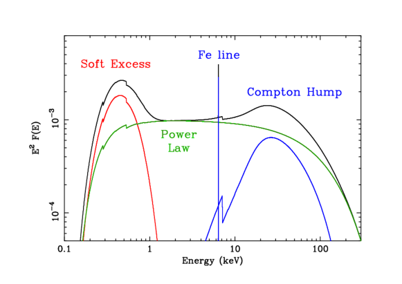
Figure 5: Schematic view of AGN X-ray spectrum in the energy range 0.1 keV $<E<$ 300 keV [216, 217]. Customarily, the ordinate shows the radiation flux scaled by $E^{2}$, so that the central part of the power-law component (see the green line) becomes approximately horizontal.

The AGN SED peaks in the UV band (near 10 eV or 1240 Å). This peak, known as the big blue bump, is traditionally associated with the expected peak of the accretion-disk thermal emission [154]. In some quasar spectra, the big blue bump was indeed well modelled by the Shakura–Sunyaev accretion disk model [156]. However, for most AGN and quasars, the peak in the SED is not as sharp as would be predicted by an accretion-disk thermal emission, and other model components are needed to explain SED towards infrared and X-ray band. The observational obstacle is the fact that at the energy range of 13.6 eV – 0.1 keV, the emission is so obscured by the Galactic interstellar gas.

X-rays and $\gamma$-rays

The AGN X-ray emission comes from the closest neighborhood of the supermassive black hole and possesses the most relevant evidence about the central source. The primary X-ray emission has a power-law like shape and it is dominated by the inverse Compton scattering of accretion-disk thermal photons in radio-quiet AGN, while the boosted jet emission prevails the spectrum in radio-loud sources (see Sec. 2.2). The X-ray power-law radiation is partly reprocessed at the accretion disk surface. The main imprints of such X-ray reflection are the iron line and the Compton hump, for a review, see e.g., Reynolds and Nowak, [563], Turner and Miller, [646]. A schematic figure of the typical AGN X-ray spectrum is shown in Figure 5.

The soft X-ray part of the AGN spectrum often exhibits an excess that can be due to ionized reflection [148] or due to Comptonization of thermal photons in a warm corona in contrast to the hot corona that creates power-law going to harder X-rays [181]. The soft X-ray emission is very often subjected to a mildly ionized absorption due to the so-called warm absorber. The absorption lines are often observed blueshifted, indicating an outflow of the warm absorber. In the most extreme cases, the outflow reaches $v_{\rm outflow}\approx 0.3$ c [643]. Such outflows are referred to as UFOs (ultra-fast outflows).

The very hard X-ray emission of radio-quiet AGN is very weak. The primary X-ray power-law is diminished by an exponential decrease of the flux around the so-called cutoff energy, as predicted by the Comptonization models. The first measurements of the cutoff energy suggest it to differ from source to source, usually it is over 100 keV [218].

AGN with significant $\gamma$-ray emission are typically radio-loud objects, indicating the origin of the $\gamma$-rays in relativistic jets. The mechanism producing $\gamma$-rays is most likely the inverse Compton upscattering of either low-frequency synchrotron photons of the jet emission or thermal photons of an accretion disc. The most luminous $\gamma$-ray sources are blazars. These sources have their collimated jets pointed towards us and the emission is strongly boosted by the Doppler beaming effect. Depending on the strength of broad emission lines, blazars can further be distinguished into BL Lac sources that lack optical emission lines (or they are only very weak) and flat-spectrum radio quasars (FSRQ) that exhibit prominent broad emission lines in their optical spectra. The $\gamma$-ray emission of blazars is variable on short timescales of the order of days and even hours, which suggests the compact size of $\gamma$-ray emitting zones, see e.g. Britzen et al., [98]. In addition, several sources exhibit a significant correlation between the radio and the $\gamma$-ray emission, with the radio emission lagging behind the high-energy emission, suggesting a spatial separation of $\gamma$-ray and radio-emission unit opacity zones as disturbances propagate downflow the jet [418], but also vice versa in some cases [97, 547], which implies the existence of two separate emission zones for the low- and high-energy radiation production.

1.2 AGN variability

AGN were found variable across all wavelengths with different amplitudes [651, 653, 655]. In general, when the source is observed in a certain waveband over time, the simplest way to represent its variability is to show its light curve, i.e. display $N$ flux densities $f_{i}$ at specific times $t_{i}$.

The variability is mainly related to primary sources of the radiation, in particular, the thermal emission of the accretion disk or the non-thermal emission of the jet. In addition, there is also variability of secondary emission sources that are powered by the emission of primary sources, for instance, the free-free emission of photo- or collisionally ionized broad-line region clouds (see Subsection 1.4). In that case, the light curve of the secondary emission is significantly correlated with the primary emission light curve, and can be used to derive the scales of the emission regions, such as the extent of broad line region. The method is known as the reverberation mapping ans is discussed in more detail in Subsection 1.4.

The AGN variability can be studied using different formalisms, each of which has its strengths as well as weaknesses. One of them is the structure function (SF), which transforms the light curve to the variability amplitude-timescale space and SF can be constructed in the following way. For each flux density $f_{i}$ at time $t_{i}$, we calculate the difference of logarithms for each flux $f_{j}$ at later times $t_{j}$, $\delta\log{F}(\delta t)=\log{(F_{j}/F_{i})}$ where $\delta t=t_{j}-t_{i}$. The structure function is then defined as the mean absolute value of $2.5\delta\log{F(\delta t)}$, in other words the mean absolute value of the magnitude difference over different time intervals. A more precise definition of the structure function is based on the decomposition of the flux into the signal and noise components, $f_{i}=s_{i}+n_{i}$, with the corresponding variances $\sigma_{s}^{2}$ and $\sigma_{n}^{2}$. The definition stems from the covariance $\mathrm{cov}(s_{i},s_{j})$ of the light curve with its time-shifted copy by time $\Delta t=t_{i}-t_{j}$ (in the rest frame of the source). In particular [360],

$$\mathrm{SF_{1}}(\Delta t)^{2}=2[\sigma_{s}^{2}-\mathrm{cov}(s_{i},s_{j})]+2\sigma_{n}^{2}\,.$$ (4)

Using the measured light curves, the structure function is commonly estimated as,

$$\mathrm{SF_{2}}(\Delta t)^{2}=\frac{1}{N_{\Delta t\text{pairs}}}\sum_{i=1}^{N_{\Delta t\text{pairs}}}(f_{i}-f_{j})^{2}\,,$$ (5)

where $\mathrm{SF_{1}}(\Delta t)^{2}=\mathrm{SF_{2}}(\Delta t)^{2}-2\sigma_{n}^{2}$, i.e. one needs to subtract correctly the noise variance $\sigma_{n}^{2}$. If this is not done properly, the structure-function slope may be flatter than it should be from basic theoretical and modelling principles, see Kozłowski, [360] for details.

The variability level can also be characterized using the mean fractional variance, which is defined as,

$$F_{\rm var}=\frac{\sqrt{\sigma^{2}-\delta^{2}}}{\langle f\rangle}\,,$$ (6)

where $\langle f\rangle$ is the mean flux density of $N$ measurements,

$$\langle f\rangle=\frac{1}{N}\sum_{i=1}^{N}f_{i}\,.$$ (7)

The flux density variance $\sigma^{2}$ can then be calculated as,

$$\sigma^{2}=\frac{1}{N}\sum_{i=1}^{N}(f_{i}-\langle f\rangle)^{2}\,,$$ (8)

while the mean square flux uncertainty is simply expressed as,

$$\delta^{2}=\frac{1}{N}\sum_{i=1}^{N}\delta_{i}^{2}\,.$$ (9)

The mean fractional variance expressed by Eq. (6) corrects for the flux measurement uncertainties, and in this sense, it estimates the true intrinsic AGN variability. It is also referred to as the excess variance.

The AGN variability is aperiodic and driven by a stochastic process in most cases [655]. However, there are a few cases when on top of the stochastic variability, one can also detect a quasi-periodic flux density changes. Such a periodic process can be driven by the accretion-flow perturbations due to a bound perturber, in particular a secondary supermassive or an intermediate-mass black hole, a neutron star, or even a wind-blowing main-sequence star. Suková et al., [622] present a general relativistic magnetohydrodynamic model for the accretion-disc perturbations driven by a bound companion and discuss the connection to several observed sources, both active galactic nuclei and quiescent SMBH, such as Sgr A*, where stars with pericenter distances of a few 100 gravitational are already detected [526, 527].

The power spectral density (PSD) allows one to study the nature of the stochastic mechanism as well as on which timescales most of the variability occurs. To construct the PSD, we need to obtain the Fourier transform of the light curve $C(t)$, which is by default in the time domain. $\tilde{C}(\nu)$ in the frequency domain is:

$$\tilde{C}(\nu)=\int_{-\infty}^{+\infty}C(t)\exp{(-i2\pi\nu t)}\mathrm{d}t\,.$$ (10)

The PSD is then obtained by the multiplication of $\tilde{C}(\nu)$ by its complex conjugate $\tilde{C}^{*}(\nu)$. Over a certain temporal frequency range ($\nu$ is expressed in Hz or day^-1), the PSD can be well fitted by a single power-law function, i.e.,

$$\text{PSD}\propto\nu^{\alpha}\,,$$ (11)

where $\alpha\leq 0$. Over a broader frequency range, from the smallest frequencies (longest timescales) to the highest frequencies (shortest timescales), PSD is generally described as a broken power-law function with one or two break frequencies. This stems from the fact that the total power is obtained by integrating over all frequencies and it needs to be finite. In particular, by integrating from a fixed frequency to the highest frequencies, it is required to have $\alpha<-1$ for convergence, while integrating towards the smallest frequencies, the power-law slope needs to increase, i.e. $\alpha>-1$. Hence, at least two power-law frequency breaks are expected. The general PSD shape is sketched in Figure 6. From the general shape, $\text{PSD}\propto 1/f^{1-2}$, it is evident that most of the variability occurs on longer timescales (small temporal frequencies). At intermediate frequencies, between the PSD frequency breaks at $\nu_{\rm b1}$ and $\nu_{\rm b2}$, the PSD shape is mostly driven by the “red-noise” process with the PSD slope of $-1$, while at higher frequencies, it gets steeper with the slope of $-2$, which is described well by the damped random walk process [DRW; 340, 400]. At low frequencies, the PSD is nearly independent of the frequency, which is typical of the “white noise". Mock light curves can be generated from the assumed PSD broken power-law shape using the Timmer–Koenig algorithm (see Timmer and Koenig, [640] for details).

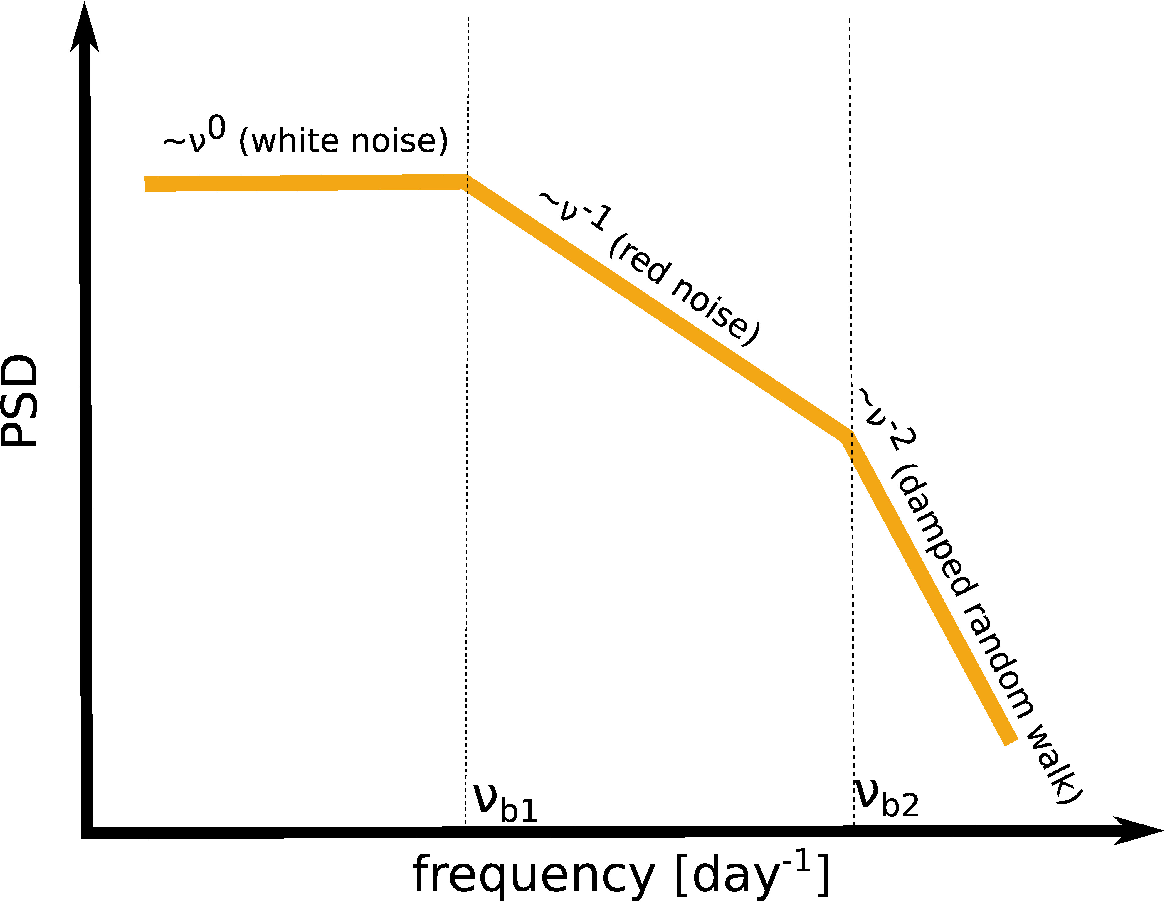
Figure 6: An illustrative power spectral density (PSD) shape described as a broken power-law function with two spectral breaks, $\nu_{\rm b1}$ and $\nu_{\rm b2}$. At low frequencies, the PSD is dominated by the flat “white”-noise process, while at the highest frequencies, the slope steepens to $-2$ and the PSD is modelled well by the damped random walk (DRW) process. At intermediate frequencies, between $\nu_{\rm b1}$ and $\nu_{\rm b2}$, the PSD is dominated by the “red” noise process with the slope close to $-1$.

The two PSD breaks are difficult to capture observationally, as at low frequencies, the timescales are too long, which requires a long monitoring program. On the other hand, at high frequencies, the short timescales are difficult to capture because of the constraints on the signal-to-noise ratio, i.e. the shorter the timescale is, the larger the observational noise. The break frequency between $\sim\nu^{-1}$ and $\sim\nu^{-2}$ is generally observed for both AGN and stellar-mass black holes, with the typical characteristic timescale of $T_{\rm B}=1/\nu_{\rm B}$ of days for SMBHs and seconds for stellar-mass black holes. The second break indicated in Figure 6 between $\sim\nu^{-1}$ and $\sim\nu^{0}$ has been mainly confirmed for stellar-mass black holes at low frequencies (long timescales).

The characteristic variability timescale $T_{\rm B}$ has empirically been determined to be proportional to the black hole mass and indirectly proportional to the accretion rate [650, 422],

$$T_{\rm B}\propto\frac{M_{\rm BH}^{1.12}}{\lambda_{\rm Edd}^{0.98}}\,,$$ (12)

where $\lambda_{\rm Edd}=L_{\rm bol}/L_{\rm Edd}$ is an Eddington ratio, i.e. the ratio between the bolometric luminosity $L_{\rm bol}=\eta\dot{M}c^{2}$ and the Eddington accretion rate $L_{\rm Edd}=4\pi GM_{\rm BH}m_{\rm p}c/\sigma_{\rm T}$, see also Eq. (22) and the related text for the derivation. The Eddington ratio can then be expressed $\lambda_{\rm Edd}\propto\dot{M}/M_{\rm BH}$, which leads to the relation between the characteristic variability timescale $T_{\rm B}$, the black hole mass $M_{\rm BH}$, and the accretion rate $\dot{M}$,

$$T_{\rm B}\propto\frac{M_{\rm BH}^{2.1}}{\dot{M}^{0.98}}\sim\frac{M_{\rm BH}^{2}}{\dot{M}}\,,$$ (13)

which is valid for accreting SMBHs as well as quiescent stellar binaries [650, 422] and can be referred to as “variability fundamental plane”.

Since $T_{\rm B}\propto M_{\rm BH}$ the variability timescale (break frequency) has been associated with the standard timescales of an accretion disc. However, the orbital dynamical timescale $t_{\rm dyn}$ is too short for AGN, of the order of hours, while the viscous timescale $t_{\rm vis}$ for an efficient accretion tends to be too long, of the order of years given $H/R\ll 1$. The association of the break frequency with the thermal instability timescale is more promising [422]. In addition, radial accretion flow fluctuations propagating from outer radii inwards have also been successful in interpreting the PSD frequency break [398, 132]. Another interpretation is the association of the characteristic variability timescale with the viscous timescale at the truncation radius, $t_{\rm vis}\sim t_{\rm dyn}\alpha_{\rm ss}^{-1}(H/R)^{-2}$, where $\alpha_{\rm ss}$ is the $\alpha$-viscosity parameter of the geometrically thin, optically thick Shakura–Sunyaev disc [599]. At the truncation radius, the optically thick disc transitions into geometrically thick and optically thin adiabatically dominated accretion flow [710]. The viscous timescale depends on the accretion rate, which determines the position of the truncation radius and in this sense the dynamical timescale. The height-to-thickness ratio $(H/R)$ also depends on the accretion rate, in particular, for accretion rates close to and exceeding the Eddington rate, the flow is geometrically puffed up and transitions into the slim disc solution with $H/R\sim 1$ [421, 374]. In this way, the viscous timescale can be altered by the accretion state. Finally, the characteristic variability timescale could be determined by the characteristic timescale of the production of hard X-rays, specifically, by the cooling timescale of electrons in the Comptonization radiation process that is responsible for the production of the hard X-ray power-law spectral distribution. According to the derivation by Ishibashi and Courvoisier, [309] based on the first principles, the cooling timescale of hot-corona electrons that are responsible for the upscattering of soft seed photons follows the same dependency as indicated by Eq. (13).

1.3 AGN structure and the unification scenarios

A large and stable luminosity that is comparable and often outshines the whole galaxy is best explained by an infall of matter – gas and dust – through the potential well of a very compact concentration of matter. For an object with mass $M$ and radius $R$, on which a matter of mass $m$ falls from infinity onto its surface, the released gravitational potential energy is,

$$\Delta E_{\rm grav}=G\,\frac{Mm}{R}\,.$$ (14)

This energy source can be compared to other relevant source of energy – the thermonuclear fusion. For the conversion of hydrogen of mass $m$ into helium, the released energy would be

$$\Delta E_{\rm nuc}\simeq 0.007mc^{2}\,.$$ (15)

The ratio of the gravitational and nuclear energies is essentially the function of the dimensionless mass-to-radius ratio $GM/Rc^{2}$, which is also denoted as compactness parameter, defined by

$$\epsilon\,\equiv\,\frac{GM}{Rc^{2}},$$ (16)

where $R$ is a typical length-scale of the system. This compactness parameter can be expressed also as

$$\frac{\Delta E_{\rm grav}}{\Delta E_{\rm nuc}}\simeq 143\,\epsilon.$$ (17)

For black holes, the typical length-scale is given by the gravitational radius,

$$R_{\rm g}=\frac{GM}{c^{2}}\simeq 1.5\times 10^{13}\,M_{8}\,\rm{cm}$$ (18)

($M_{8}{\equiv}{M}/10^{8}M_{\odot}$). For high compactness, the release of gravitational potential energy can be even two orders of magnitude larger than the energy available via thermonuclear fusion. For black holes, the compactness ratio is naturally the largest. For neutron stars with the mass of $M\approx 1\,M_{\odot}$ and radius of $R\approx 10\,{\rm km}$, the compactness parameter is $\epsilon=GM_{\rm NS}/(R_{\rm NS}c^{2})\approx 0.1$, which yields $\Delta E_{\rm grav}/\Delta E_{\rm nuc}$ of the order of 10. In case we fix the mass of the gravitating object to one solar mass, $M=1\,M_{\odot}$, the ratio $\Delta E_{\rm grav}/\Delta E_{\rm nuc}$ is equal to unity for the radius of $R=200\,{\rm km}$, i.e. for all other stable astrophysical objects the thermonuclear fusion is more efficient source than the release of the gravitational potential energy . For sun-like stars, the ratio $\Delta E_{\rm grav}/\Delta E_{\rm nuc}\simeq 10^{-4}$, i.e. the accretion yield is several thousand times smaller than the thermonuclear yield. Nevertheless, even for main-sequence stars the accretion can be of importance in symbiotic systems where the matter is transferred from one star to the other.

On the other hand, in binary stellar systems that contain a white dwarf, a fast thermonuclear fusion on the surface can be visible as a bright nova and generally outshine the luminosity due to the accretion. The important quantity for all energy-generation processes is the timescale $\tau$, on which the energy $\Delta E$ is released. The total bolometric luminosity across the whole electromagnetic spectrum can then be defined as,

$$L=\frac{\Delta E}{\tau}$$ (19)

Let us note that another dimensionless quantity can also be denoted as the compactness parameter in the theory of accretion onto compact objects [120],

$$\tilde{\varepsilon}\equiv\frac{L\,\sigma_{\rm T}}{Rm_{\rm e}c^{3}}$$ (20)

with Thomson cross-section for electrons is $\sigma_{\rm T}=6.65\,246\times 10^{-25}\;{\rm cm}^{2}$; $\tilde{\varepsilon}$ has an advantage of taking the effects of radiation pressure into account.

Considering the symmetric stationary accretion on a compact object – assuming a supermassive black hole (hereafter SMBH) of mass $M_{\bullet}$ – it is possible to derive a useful analytic expression for the maximum accretion luminosity, for which the stationary symmetric accretion stops to proceed. Let us assume that the black hole is surrounded by the ionized hydrogen gas. In that case the radiation pressure force mainly acts on electrons via the Thomson scattering, since for protons the scattering is smaller by a factor of $(m_{\rm e}/m_{\rm p})^{2}$. Since the electron and the proton are bound by a Coulomb force, the radial outward radiation force acting on the whole pair can be calculated as $F_{\rm rad}=\sigma_{\rm T}S/c$ (rate of momentum absorption), where $S$ is the bolometric radiation flux, $S=L/(4\pi r^{2})$, and $c$ is the speed of light. The Coulomb pair is attracted inwards mainly due to the proton-black hole gravitational interaction $F_{\rm grav}=GM_{\bullet}(m_{\rm p}+m_{\rm e})/r^{2}\simeq GM_{\bullet}m_{\rm p}/r^{2}$. Finally, the total inward force acting on the electron-proton pair can be calculated as,

$$F_{\rm tot}\simeq\frac{1}{r^{2}}\left(GM_{\bullet}m_{\rm p}-\frac{\sigma_{\rm T}L}{4\pi c}\right)\,.$$ (21)

The total force is zero when the term in parentheses disappears, which is for the luminosity,

$$L_{\rm Edd}=\frac{4\pi GM_{\bullet}m_{\rm p}c}{\sigma_{\rm T}}=1.3\times 10^{46}\left(\frac{M_{\bullet}}{10^{8}\,M_{\odot}}\right)\,{\rm erg\,s^{-1}}\,.$$ (22)

Expression given by Eq. (22) is referred to as the Eddington luminosity, a.k.a. the Eddington limit. This limit was derived under the assumption of the steady spherical accretion, which is in real systems quite unrealistic since the accretion proceeds in the axially symmetric disks in the first approximation as will be discussed in Section 2 in more detail.

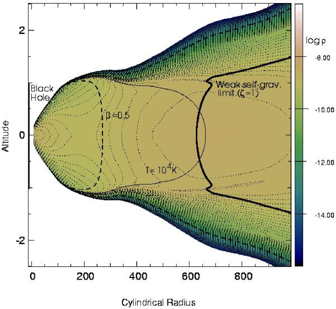
Figure 7: The geometrical profile in the azimuthal ($\phi={\rm const}$) section and the distribution o density (color coded in arbitrary units) within the accretion torus feeding a $M_{\bullet}=10^{8}M_{\odot}$ SMBH [figure adapted from 305]. The black hole is located in the center of the matter distribution. The gaseous environment becomes weakly self-gravitating beyond the radius $\approx 6\times 10^{2}\,GM_{\bullet}/c^{2}$, as characterized by the Toomre criterion and indicated by the numerically constructed $\zeta=1$ contour [for further details, see ref. 323].

However, the Eddington limit still serves as a useful value with which the observed bolometric luminosity $L_{\rm bol}$ is compared. The ratio of the observed luminosity to the Eddington luminosity is called the Eddington ratio, $\lambda_{\rm Edd}\equiv L_{\rm bol}/L_{\rm Edd}$. In order to calculate the Eddington ratio, one first needs to convert the luminosity in a given wavelength (frequency band) to the bolometric luminosity, using the SED of a given AGN spectral class, see also Fig. 2. The calculation of the Eddington ratio also requires the determination of the supermassive black hole mass $M_{\bullet}$, for which more methods can be employed, depending on the AGN host type and the redshift of the source. These methods will be summarized later in this Subsection.

In general, the observations show that the AGN luminosity in most galaxies is sub-Eddington, $\lambda_{\rm Edd}<1$. For low Eddington ratios, $\lambda_{\rm Edd}\leq 0.3$, the optically thick and geometrically thin accretion disks provide good fits to the SED of the AGN [356, 79, 169]. For higher accretion rates, the disk turns into the geometrically thick or “slim” mode, with the effects of photon trapping and advection becoming relevant [see Fig. 7; 3, 579, 187, 671]. The slim accretion disks with super-Eddington luminosities, $\lambda_{\rm Edd}\geq 1$, have different SED properties than standard thin disk, mainly the high-energy cut-off and the strong anisotropy in the emitted radiation, which is expected to arise due to the self-shadowing of the inner parts of slim disks [673].

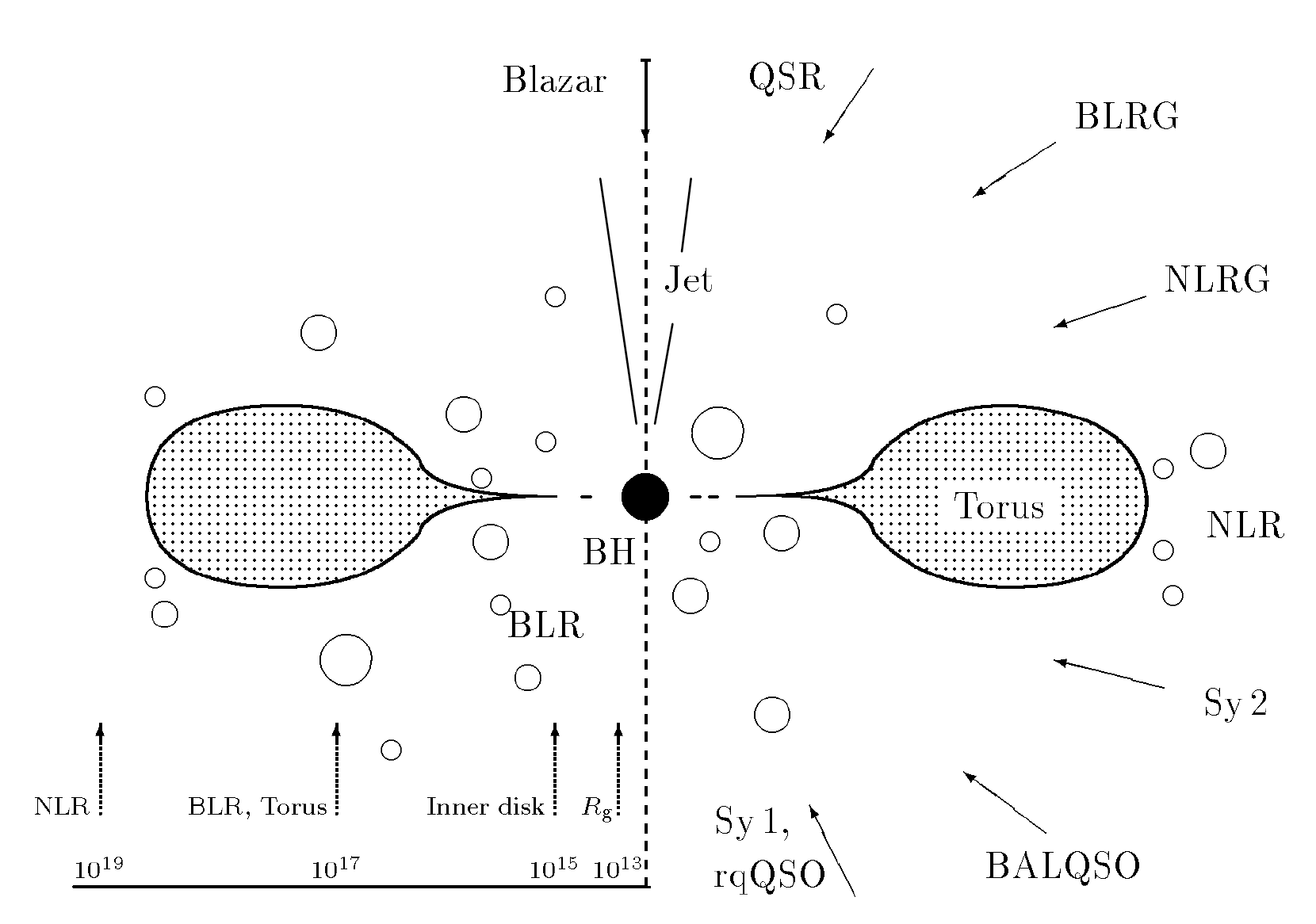
Figure 8: A schematic picture of AGN unification. Radio-quiet sources are divided into two groups of Seyfert 1 (a.k.a. Sy1) and Seyfert 2 (Sy2) types, as shown at the bottom, while radio-loud galaxies (shown in the top) are distinguished also according to the kinetic power of the jet and its orientation with respect to the observer. Notes: FR I and II are radio galaxies with the morphology according to the Fanaroff–Riley classification. NLRG are Narrow-Line Radio Galaxies, BLRG are Broad-Line Radio Galaxies, and FSRQ are Flat-Spectrum Radio Quasars.

AGN have various appearances of their electromagnetic spectrum. The most prominent distinction among different AGN kinds is at the radio band, where the flux of radio-loud and radio-quiet AGN differs by several orders of magnitude. The radio-loud AGN are associated with sources launching a powerful and collimated relativistic jet from the close vicinity to the supermassive black hole (see Section 3). The other major distinction of different AGN kinds is the presence/absence of the broad emission lines and suppressed continuum of the obscured sources. The suppressed continuum and the absence of broad emission lines are related and caused by a large obscuration of the central region by a dusty circumnuclear structure, called torus.

The optical polarization measurements reveal that the broad wings of the lines are not completely absent in type-II objects. The broad lines that are otherwise hidden in the total spectra have appeared in the polarized spectra because the polarized emission originates by the scattering of the central-region photons at the polar region. The polarization thus served as a tool to view the central region of type-II AGN like via a periscope. These measurements proved that the obscured type-II sources have also the same central region as unobscured type-I AGN, which led to the first AGN unification explaining the difference between different kinds of AGN based on the various viewing angle [23, 648]. Type-I AGN are viewed from “above”, while type-II AGN are viewed from the edge and thus with the line-of-sight intercepting the torus.

Figure 8, adopted from Beckmann and Shrader, [52], schematically shows the unification scenario for radio-quiet (bottom) as well as radio-loud AGN (top). The figure displays the main constituents of AGN. There is a supermassive black hole in the centre surrounded by an accretion disk and electron plasma. About 10% of the sources also have a strong relativistic jet and are radio-loud sources. The emission lines originate in the broad-line and narrow-line regions. The narrow-line region is more distant and is always visible. However, the broad-line region can be hidden at some high-inclined orientations. The direct emission from the central region is visible in type-I objects, while this radiation is absorbed and only partly transmitted through a torus in type-II objects. The dominant emission in type-II sources might be the reflected emission at the torus and the scattered emission in the narrow-line region. The broad-line region is thus well visible only for low-inclined sources.

A special class of AGN are blazars that are pointing their jets directly towards the observer. Due to the strong relativistic beaming, the whole SED of blazars is dominated by the emission from the jet. The blazars can be divided into two groups – BL Lac and FSRQ (Flat-Spectrum Radio Quasars). The difference between these two classes is in radio properties (FSRQ having a flat spectral index), but mainly in the presence of the prominent broad optical emission lines in FSRQs, while they are missing in BL Lac sources. The most accepted explanation for the difference between these two classes is the difference between their accretion rates. While BL Lac sources are supposed to be in an inefficient accretion mode with not enough radiation to photoionize and create the broad-line region clouds, FSRQs are highly-accreting luminous sources with a significant thermal emission from accretion disks sufficient to create and photoionize the broad-line region [234, 407].

The accretion rate is clearly another factor playing a significant role in the AGN classification. Similarly to the absence of the broad emission lines in BL Lac sources, also some Seyferts show the lack of the broad emission lines in their spectra, while they do not show any evidence of obscuration due to the torus blocking the view to the central region. Such sources are known as true-type-II Seyferts [518, 68], and may represent low-accreting AGN with absent or not sufficiently illuminated broad-line region clouds.

Let us note that the radio-loud AGN can be divided according to their jet power. Their morphological classification was proposed to correspond to FR-I type according to Fanaroff–Riley when the radio emission arises from a compact region. Oppositely, the high-power sources were proposed to correspond to FR-II type, where the most radio emission origintace from extended radio lobes. Alternatively, it hes been proposed that the FR classification might be related to the properties of the intergalactic medium rather than the intrinsic properties of the jet.

The circumnuclear obscurer is not a homogeneous body (as was already discussed in previous Section reviewing the infrared observations of AGN), but is rather formed by individual clumps. Therefore, it can happen that a clear view of the central region is possible in some sources also from a relatively high inclination, depending on the actual distribution of the obscuring clouds. And because the whole structure is dynamic (the clouds are in a motion), AGN types can vary from one type to the other. The change of the spectral type of an AGN was indeed observed several times, most prominently by sources called changing-look AGN [372, 401]. However, it was argued that variable absorption due to passing clouds can hardly explain variability seen in the large extended optical region of AGN emission and the intrinsic changes of the accretion flow were suggested to be more credible interpretation [372, 492].

The basic AGN classification on type-I and type-II sources is not ubiquitous at any wavelength. Although the obscuration in the optical and X-ray energy domain was found to be related [261, 108], it was shown by Merloni et al., [431] on a large AGN sample that only about 70% AGN in fact agree on the optical and X-ray classification. The rest 30% can be divided in two sub-groups: (i) to low-luminosity objects that are X-ray unobscured but lack the broad lines, and (ii) luminous AGN with the broad lines but with prominent X-ray absorption.

The presence of the supermassive black hole in AGN cores was historically proposed to explain large megaparsec scales of jets in quasi-stellar objects (QSOs) as well as the measured emitted large energies and the variability on very short-timescales. Let us briefly summarize here the main arguments:

• For several radio sources, the measured jet sizes reach several megaparsecs, $L\approx 10^{6}\,{\rm pc}$. Taking the upper limit of the expansion speed as the speed of light $c$, we obtain the lower limit for the age of the central engine, $\tau>L/c\approx 10^{6}\,{\rm pc}/3\times 10^{8}\,{\rm m\,s^{-1}}\approx 3\times 10^{6}\,{\rm yr}$.

• Luminous quasars can reach bolometric luminosities of $L_{\rm QSO}\approx 10^{47}\,{\rm erg\,s^{-1}}$. Then the minimum emitted energy over the engine lifetime is, $E_{\rm QSO}\approx L_{\rm QSO}\tau\approx 10^{61}\,{\rm erg}$.

• Typical AGN are variable sources on all timescales, even as short as one day and less; $\tau_{\rm{var}}\approx 1\,{\rm day}$. This timescale sets an upper limit on the emitting region since the maximum velocity with which the changes can take place is the speed of light $c$ in order for the whole emitting region to be causally connected. Then the maximum length-scale can be inferred from a light travel time of the order of a few days, $R_{\rm emit}\lesssim\tau_{\rm var}c\approx 1\,{\rm day}\times 3\times 10^{8}\,{\rm m\,s^{-1}}\approx 2.6\times 10^{13}\,{\rm m}\approx 1{\rm mpc}=170\,{\rm AU}$.

Hence, the central engine has the length-scale of the Solar System and needs to be stable enough for at least millions of years and be able to produce luminosities of the order of $10^{13}\,L_{\odot}$. However, the mechanism of transferring the gas from the outer parts of the galaxy towards the nucleus and then feeding the central black hole remains the subject of many debates [618]. It appears that the estimated rate of mass inflow, about 0.01 to a few solar masses per year, is often higher by three orders of magnitude than the mass accretion rate onto the central SMBH. A question arises what the actual mass of such a compact and energetic system is. The mass estimates may be derived from the assumption of the virial theorem that should hold for the self-gravitating systems of gas, dust and stars in hydrostatic equilibrium. i.e. those that neither contract nor expand.

The virial theorem may simply be derived for bound orbits of gas and stars that orbit black holes in the centre of galaxies. The characteristic Keplerian velocity is given from the Newtonian theory by setting the centripetal force ($mv^{2}/r$) acting on an object equal to the gravitational force ($GM_{\bullet}m/r^{2}$):

$$v_{\rm K}=\sqrt{GM_{\bullet}/r}\,.$$ (23)

Accreting matter forms a disk-like structure, which consists essentially of many individual elements; we can imagine them as discrete blobs of plasma, each one moving along an (approximately) Keplerian orbit with the characteristic velocity $v(R)=v_{\rm K}$. Due to the viscosity of the disk, blobs gradually lose the angular momentum and the gravitational potential energy while gaining the kinetic energy:

$$E_{\rm K}=\textstyle{\frac{1}{2}}mv_{\rm K}^{2}=\textstyle{\frac{1}{2}}GM_{\bullet}m/r\,.$$ (24)

The gravitational potential energy of the blob is $E_{\rm P}=-GM_{\bullet}m/r$ and the corresponding kinetic energy during the accretion process is equal to

$$E_{\rm K}=\textstyle{\frac{1}{2}}\frac{GM_{\bullet}m}{r}=-\textstyle{\frac{1}{2}}E_{\rm P}\,.$$ (25)

The total mechanical energy reads

$$E_{\rm tot}=E_{\rm K}+E_{\rm P}=\textstyle{\frac{1}{2}}E_{\rm P}\,.$$ (26)

Finally, the virial theorem for the self-gravitating system in hydrostatic equilibrium (without taking time-dependency into account),

$$2\langle E_{\rm K}\rangle_{\rm R}+\langle E_{\rm P}\rangle_{R}=0\,,$$ (27)

where the brackets $\langle...\rangle_{\rm R}$ denote the averaging over the whole dynamical system of the length-scale $R$.

The importance of the virial-theorem for the accretion onto black holes is that one-half of the loss of the potential energy is converted into the gas kinetic energy while the other half is available for the gas heating, which leads to the emission of electromagnetic radiation in the X-ray, ultraviolet, and visible domains.

The Keplerian velocity profile of the emitting material bound to the central supermassive black hole directly implies that the emission lines of the hot gas should be significantly Doppler-broadened. The observed line profile is given by the summing of the flux of all orbiting blobs or clouds around the central black hole. For some AGN, not all, very broad lines with the line widths corresponding to $<v>=10^{3}$–$10^{4}\,{\rm km\,s^{-1}}$ have been detected – these are AGN of type 1. Given the compactness of the emitting region obtained from the variability timescale, we can infer the total mass in this region from Eq. (23),

$$M_{\rm center}=\frac{\langle v\rangle\;^{2}R}{G}\approx 10^{5}\mbox{--}10^{7}\,M_{\odot}\,.$$ (28)

Based on the virial theorem, Eq. (27), the accretion luminosity can be expressed as,

$$L_{\rm acc}=\frac{1}{2}\frac{GM_{\bullet}\dot{M}_{\rm acc}}{R_{0}}\,$$ (29)

where $R_{0}$ is the initial radius, from which the matter falls onto the compact object. In case of black holes, naturally infalling matter does not hit any surface but passes through the event horizon. In accretion disks around black holes, hot gas spirals in due to the extraction of the angular momentum, until it reaches the innermost stable circular orbit (ISCO). Subsequently, the matter falls into the black hole since no stable orbit exists inside the ISCO. Therefore, we can set $R_{0}=R_{\rm ISCO}$. For a non-rotating black hole, we have $R_{0}=6GM_{\bullet}/c^{2}$ and the accretion luminosity becomes,

$$L_{\rm acc}=\eta\dot{M}_{\rm acc}c^{2}\,,$$ (30)

where $\eta=1/12$, i.e. the efficiency for a non-rotating black hole is $8.3\%$ and the correct relativistic calculation would give $\sim 5.7\%$ for an accretion from a thin accretion disk. For a maximally rotating black hole, $R_{\rm ISCO}=GM_{\bullet}/c^{2}$, which yields $\eta=1/2$, however the general relativistic calculation again gives a smaller value of $\sim 29\%$. We see that the accretion efficiency $\eta$ can reach values as large as $\sim 10\%$, which is one order of magnitude larger than the efficiency of the energy release via the thermonuclear fusion, $\epsilon\lesssim 0.8\%$, where the uppermost limit corresponds to the the conversion of hydrogen into iron. In other words, the energy released through the thermonuclear fusion of hydrogen is $\sim 6\times 10^{6}\,{\rm eV}$ per hydrogen atom, while the accretion from a thin disk on a non-rotating black hole yields the energy rate larger by one order of magnitude.

If we take $\eta=0.1$, then the accretion rate for typical quasar luminosities of $L_{\rm acc}\approx 10^{46}\,{\rm erg\,s^{-1}}$ is,

$$\dot{M}_{\rm acc}=1.8\left(\frac{L_{\rm acc}}{10^{46}\,{\rm erg\,s^{-1}}}\right)\left(\frac{\eta}{0.1}\right)^{-1}\,M_{\odot}{\rm yr^{-1}}\,.$$ (31)

This means that quasars must accrete close to the Eddington limit $L_{\rm Edd}$, see Eq. (22), when considering black holes of mass $M_{\bullet}=10^{8}\,M_{\odot}$. The Eddington accretion rate is derived by setting the accretion luminosity, Eq. (30), equal to the Eddington luminosity, Eq. (22),

$$\dot{M}_{\rm Edd} =\frac{4\pi GM_{\bullet}m_{\rm p}}{\eta\sigma_{\rm T}c}\,$$

$$\approx 2.6\left(\frac{\eta}{0.1}\right)^{-1}\left(\frac{M_{\bullet}}{10^{8}\,M_{\odot}}\right)\,M_{\odot}\,{\rm yr^{-1}}\,.$$ (32)

The stable and very compact configuration of the order of million Solar masses can be explained by the presence of supermassive black hole. Other compact objects, white dwarfs and neutron stars, are too light – white dwarfs, which are prevented from further gravitational collapse by the pressure of degenerate electrons, have the upper mass limit given by the Chandrasekhar limit,

$$M_{\rm Ch}\approx m_{\rm B}[\hbar c/(Gm_{\rm B}^{2})]^{3/2}\approx 1.4\,M_{\odot}\,$$ (33)

and neutron stars have a slightly larger, but still too small upper limit given by the Tolman–Oppenheimer–Volkoff limit, $M_{\rm TOV}\leq 3\,M_{\odot}$.

Main-sequence stars can theoretically reach the masses of the order of $100\,M_{\odot}$ when they consist purely of hydrogen and helium plasma, but they are too short-lived, less than million years. Hence, classical relativistic theories of stellar structure and evolution allow only one stable configuration to explain the characteristics of the AGN – supermassive black holes. However, quantum theories of gravity could explain the compact large concentrations using models of quantum nature (boson stars, macroquantumness). In general, the presence of the event horizon is difficult to prove by observations of the emerging electromagnetic waves [6].

The reader may consider it as strange and mysterious that black holes of $10^{6}$–$10^{10}\,M_{\odot}$ reside in the cores of luminous quasars and following the Soltan argument [614], in the nuclei of most nearby galaxies. The classical stellar theories and numerical studies show that stellar black holes are the final end-states of the stellar collapse with the remnant mass of $>3\,M_{\odot}$. The initial stellar masses have to be in excess of $45\,M_{\odot}$  depending on the stellar metallicity. Numerical studies that employ Cold Dark Matter (CDM) models show that the first stars in the early Universe were very massive, $\gtrsim 100\,M_{\odot}$, with very low metallicities [391]. The first baryonic structures started to form at the redshift of $z\sim 30$ based on the principle of the Jeans gravitational instability and they started to reionize the neutral hydrogen in their surroundings. This so-called reionization era finished at $z\sim 6$, i.e. the Universe was fully ionized at that redshift based on the quasar observations and the detection of the so-called Ly$\alpha$ forest in their spectra. The formation of first baryonic structures, such as stars and black holes, provides a transition from a rather simple, smooth state of the Universe with small, primordial density fluctuations to the current, coarse state that is full of different structures and large differences in the mass density. Necessary tools to study this transition include computationally demanding cosmological hydrodynamic simulations [102, 2] as well as the observations in the mid-infrared bands, in particular by the James Webb Space Telescope [391].

The Ly$\alpha$ forest is a set of absorption lines in the spectra of distant quasars short of the Ly$\alpha$ line at the corresponding redshift. Due to the presence of a small amount of neutral hydrogen along the line of sight, Ly$\alpha$ photons are effectively scattered and suppressed, which yields a set of absorption lines at the blueshifted part of the actual Ly$\alpha$ line. In case the ratio of neutral to ionized hydrogen in the intergalactic medium reaches larger values than $10^{-3}$, the absorption lines become largely blended and a so-called Gunn–Peterson through is formed. The Gunn–Peterson through was detected for a quasar at $z\approx 6.28$, but not for quasars at smaller redshifts [49]. This indicates that at redshift $z\sim 6$ the reionization of the Universe by the radiation of first stars and the activity of first black holes is largely completed.

So far two basic channels of the formation of black hole seeds have been investigated. One includes very massive hydrogen-helium stars (Population III) that started to form after the recombination epoch ($\sim 380\,000$ years after the Big Bang, which corresponds to the redshift $z=1100$) during the first hundred million years after the Big Bang. These very massive stars of $\sim 100$ Solar masses produced seed black holes of $10-100$ Solar masses that accreted from the local environment. The first stars formed in gaseous molecular disks that cooled mostly via $H_{2}$ cooling and fragmented subsequently and formed stars. The second scenario starts with a gaseous disk again, but instead of cooling through molecular hydrogen, it contains mainly atomic hydrogen, which is not such an efficient coolant. This scenario also includes external irradiation, which prevents molecular hydrogen from forming. The gaseous disk then becomes gravitationally unstable as a whole and the matter is channeled into the centre where the black hole is formed directly – a so-called direct collapse black hole [see also 475, for an overview and a popular account]. Natarajan, [475] describes the two scenarios, (i) on one side the formation of seed black holes from Population III stars, and (ii) the direct collapse of an externally illuminated gaseous disk on the other side. The problem of the scenario that involves Population III stars as the origin of black-hole seeds is that the black holes are not massive enough at $\sim 770$ million years after the big bang when the first quasars are expected to appear. This “under-weight” problem is solved by the model of the direct collapse of a gaseous disk, which can lead to the much faster growth of the first black holes. We illustrate both scenarios in Figure 9.

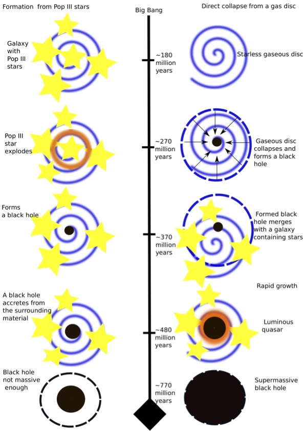
Figure 9: Two formation channels of the first massive black holes residing at the cores of the first quasars at $\sim 770$ Myr after the Big Bang: (i) the first scenario, depicted on the left, shows the formation of seed stellar black holes from Population III (Pop III) stars; (ii) the second scenario shown on the right involves a neutral, irradiated disk of hydrogen that collapses directly into a more massive black hole seed. This larger seed then merges with a cluster of Population III stars and gets quickly more massive by a rapid accretion. The second scenario is more consistent with the occurrence of the first quasars $\sim$ 770 Myr after the Big Bang. This visualisation was adapted from an inspiring article on the feedback processes by Natarajan, [475].

The basic model of the black hole growth by accretion can be constructed from the first principles. Let us assume that the black hole accretes with the efficiency of $\epsilon$ and the rate of $\dot{M}_{\rm acc}$, which yields the accretion luminosity of

$$L_{\rm acc}=\epsilon\dot{M}_{\rm acc}c^{2}\,.$$ (34)

The complementary fraction of the accretion rate contributes to the black hole mass increase,

$$\dot{M}_{\bullet}=(1-\epsilon)\dot{M}_{\rm acc}\,.$$ (35)

which can be rewritten in terms of the Eddington luminosity and the Eddington ratio using Eqs. (29), (34)

$$\dot{M}_{\bullet}=\frac{1-\epsilon}{\epsilon}\frac{L_{\rm Edd}}{c^{2}}\lambda_{\rm Edd}\,.$$ (36)

Using the Eddington luminosity, the relation (36) can be rewritten in such a way so that the mass is on the left side and the time on the other in a differential form. Subsequently, one can integrate the left side with the limits $(M_{\bullet}(0),M_{\bullet})$ and the right side with the limits $(0,t)$,

$$\int_{M_{\bullet}(0)}^{M_{\bullet}}\frac{\mathrm{d}M_{\bullet}^{\prime}}{M_{\bullet}^{\prime}}=\int_{0}^{t}\frac{1-\epsilon}{\epsilon}\lambda_{\rm Edd}\frac{4\pi Gm_{\rm p}c}{\sigma_{\rm T}c^{2}}\mathrm{d}t^{\prime}\,,$$ (37)

which after the integration yields an exponential growth model,

$$M_{\bullet}(t)=M_{\bullet}(0)\exp{\left(\frac{1-\epsilon}{\epsilon}\lambda_{\rm Edd}\frac{t}{\tau_{\rm Sal}}\right)}\,.$$ (38)

Hence the black hole mass grows exponentially with time, $M_{\bullet}\propto\exp{(t/\tau_{\rm Sal})}$, where the $e$-folding timescale $\tau_{\rm Sal}$ is the Salpeter time,

$$\tau_{\rm Sal}=\frac{M_{\bullet}c^{2}}{L_{\rm Edd}}=\frac{\sigma_{\rm T}c}{4\pi Gm_{\rm p}}\simeq 4.5\times 10^{8}\,{\rm yr}\,.$$ (39)

Apparently, $\tau_{\rm Sal}$ depends on the fundamental constants only.

The black hole growth via the accretion close to the Eddington limit, i.e. the quasar stage, is not a continuous process. This is mainly due to the feedback process, which we understand here as depositing the momentum onto the surrounding cold gas as well as its heating and ionization by intense radiation. This leads to the decrease of the amount of dense cold gas, which is needed for both the accretion as well as star-formation. This is a so-called negative feedback. Occasionally, the propagating jet leads to the shocks and the compression of the ambient gas, which can trigger star-formation (positive feedback). This complicated interplay among the cold gas reservoir, accretion/jet activity, and star-formation is illustrated in Figure 10. The negative feedback on the cold-gas reservoir can be in the form of radiative mode (wind or quasar), where the gas is expelled due to quasar winds, jet and radiation and this mode is typical of luminous AGN, or in the form of kinetic mode (radio or jet), where the cold gas is heated up and this mode occurs for low-excitation radio-loud AGN [14].

The star-formation rate is globally related to the density of gas in galaxies via the Kennicutt–Schmidt law, which expresses the star-formation rate surface density, expressed in ${\rm M_{\odot}\,yr^{-1}\,pc^{-2}}$, as a power-law function of the gas surface-density, expressed in ${\rm g\,pc^{-2}}$ [584],

$$\Sigma_{\rm SFR}=A\Sigma_{\rm gas}^{n}\,,$$ (40)

where $A$ is an absolute star-formation efficiency. Initially, according to the analysis of Schmidt, [584], $n$ was found to be $\approx 2$ close to the Solar neighbourhood based on the abundance of helium and the occurrence of white dwarfs. Using the sample of HI, CO, $H\alpha$ spiral galaxies and CO and far-infrared starburst galaxies, Kennicutt, [341] demonstrated that the Schmidt law expressed by Eq. (40) applies globally for one-zone models of galaxies, i.e. for a disk-averaged star-formation rate, and the power-law index was constrained to be $n=1.4\pm 0.15$.

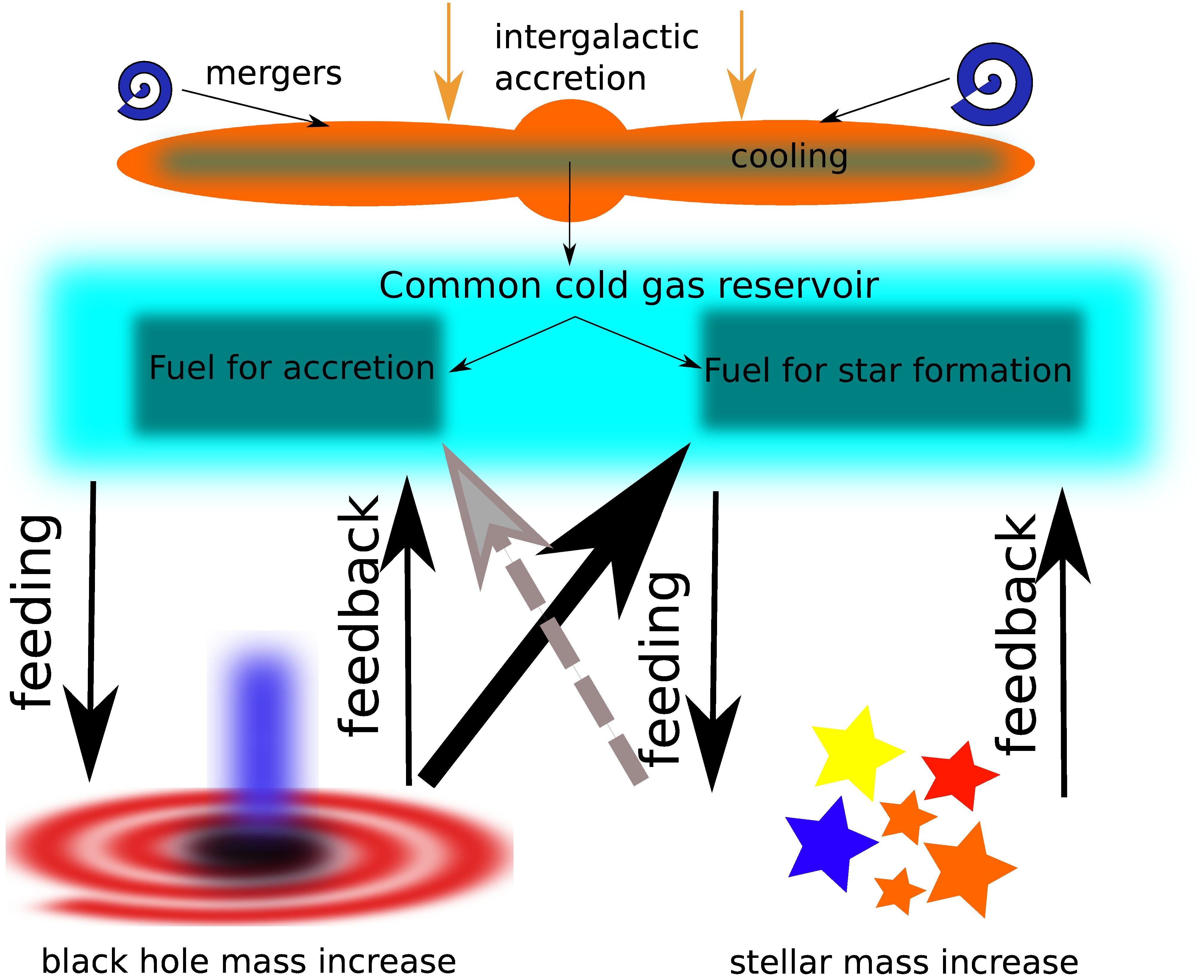
Figure 10: Illustration of the AGN feeding and feedback processes. From the top, we show the main sources of gas in an AGN host – intergalactic accretion, gas-rich mergers, and galactic sources (supernovae, stellar winds). The cold gas is formed via the radiative and the adiabatic cooling. Subsequently, it fuels the black hole accretion as well as star-formation. Both processes lead to the mechanical and radiation feedback, which both remove the cold gas and cause the drop in the accretion and the star-formation rate. This illustration was inspired by Harrison, [283] and adapted from Zajaček et al., 2020d [705]. .

1.4 AGN circumnuclear medium: the interplay of gas and stars

In this subsection, we focus on the interstellar medium in the central parts of active galactic nuclei in the context of the mutual interaction among gas, stars, and the supermassive black hole. The motion of the gaseous-dusty circumnuclear medium in the potential dominated by the central supermassive black hole (SMBH) is necessary to account for broad emission lines with line widths of the order of several $1000\,{\rm km\,s^{-1}}$. Such large line widths arise due to the Doppler-broadening of the ionized gas emission due to the dominantly orbital motion of cloudlets around the SMBH. The gas can flow in towards the SMBH inside the Bondi radius, where its gravitational potential prevails over that of the thermal gas pressure of temperature $T_{\rm g}$,

$$r_{\rm Bondi}\approx\frac{GM_{\bullet}}{c_{\rm s}^{2}}=1\,\left(\frac{M_{\bullet}}{2\times 10^{8}\,M_{\odot}}\right)\left(\frac{T_{\rm g}}{10^{8}\,{\rm K}}\right)^{-1}\,{\rm pc}\,,$$ (41)

which eventually sets the basic length-scale of the region of our interest. Whether in free-fall as in the spherical Bondi accretion, for which the matter has lost its angular momentum, or already circularized gas with the initial angular momentum, the velocities of the order of $\sim 1000\,{\rm km\,s^{-1}}$ are reached already well before reaching the innermost stable circular orbit (ISCO) of the central black hole,

$$r_{\rm BL,kin}=f\frac{GM_{\bullet}}{v_{\rm K}^{2}}=0.86f\left(\frac{M_{\bullet}}{2\times 10^{8}\,M_{\odot}}\right)\left(\frac{v_{\rm K}}{1000\,{\rm km\,s^{-1}}}\right)^{-2}\,{\rm pc}\sim 45\,000f\,R_{\rm s}\,,$$ (42)

where $f$ is the kinematical/geometrical factor of the accreting gas and $R_{\rm s}$ represents the Schwarzschild radius of the SMBH, $R_{\rm s}=2GM_{\bullet}/c^{2}=1.9\times 10^{-5}(M_{\bullet}/2\times 10^{8}\,M_{\odot})\,{\rm pc}$. This gives a basic estimate of the mean kinematic radius of the broad-line region, which is comparable to the Bondi radius in Eq. (41).

We will refer in the following analysis to both the interstellar and the circumnuclear medium of active galactic nuclei (AGN) interchangeably. This stems from the fact that stars as members of dense nuclear star clusters (NSCs) typically do not appear as one of the components in the unified AGN models [24, 648]. However, they are expected to be present and can actually provide a fraction to both the accreted matter and the outflow [60, 689] or at least they are expected to influence hydrodynamics in the central regions of galaxies. In fact, nuclear star clusters have been detected at the photometric as well as dynamical centers of a significant fraction (60$\%$-75$\%$) of both early-type and late-type galaxies in the local Universe [118, 89, 145, 486]. In general, they are thought to co-evolve with massive black holes at galactic centers, where they mutually influence their growth [485]. Having typical effective radii of a few parsecs and the total masses of a few $10^{5}$–$10^{8}\,M_{\odot}$, NSCs are one of the densest stellar systems in galaxies [90, 666, 587] with the mean surface densities up to $\sim 10^{5}\,M_{\odot}\,{\rm pc^{-2}}$, similar to globular clusters and other compact stellar systems, but brighter. In addition, there is an evidence of co-existence with active massive black holes at their centers [597, 263, 485]. Also, kinematically resolved NSCs show a Keplerian rise in velocities in their inner portions, $\sigma_{\star}\propto r^{-1/2}$. The influence radius of SMBHs $R_{\rm inf}$ is often estimated by the radius at which the Keplerian circular velocity of stars around the SMBH is equal to their one-dimensional (line-of-sight) stellar velocity dispersion,

$$R_{\rm inf}=\frac{GM_{\bullet}}{\sigma_{\star}^{2}}\approx 86\left(\frac{M_{\bullet}}{2\times 10^{8}\,M_{\odot}}\right)\left(\frac{\sigma_{\star}}{100\,{\rm km\,s^{-1}}}\right)^{-2}\,{\rm pc}\,$$ (43)

which can be larger than the NSC effective radius for massive black holes, but only as small as $\sim 2\,{\rm pc}$ for the Galactic centre black hole of $M_{SgrA*}\simeq 4\times 10^{6}\,M_{\odot}$ [587].

To what extent the NSC as a whole influences the standard parameters of AGN (black hole mass, accretion rate, accretion disc structure, broad- and narrow-line region clouds) is still not known. A self-consistent treatment of the influence of stars on the accretion disc was done by Wang et al. [672, 670], who build on the earlier models of [532, 658]. They show that stars that form beyond the self-gravitation radius in the accretion disc drive outflows of hot gas beyond the disc plane through supernova explosions. This hot gas leads to the cyclic production of broad-line region clouds as well as the metallicity gradient in the accretion disc. The general picture is more complex as the NSCs themselves experience recurrent in-situ star-formation [570], possibly depending on the cycles of cold gas inflows from larger scales. Although NSCs are spheroidal, Seth et al. [598] show that for some galaxies there are younger flattened subsystems embedded within the older spheroidal structure. Subsequent dynamical mechanisms [resonant and non-resonant relaxation processes; 434] are required to turn young stellar disks/rings into spheroidal stellar systems. Seth et al. [598] estimate the timescale of $\sim 0.5\,{\rm Gyr}$ between individual star-formation episodes.

The prominent broad emission lines associated with the broad line region (hereafter BLR) are generally observed in AGN [337, 534, 64, 274], i.e. about $\sim 10\%$ of galactic nuclei with the high accretion rate of the order of $1\,M_{\odot}\,{\rm yr^{-1}}$ in comparison with the majority of quiescent sources, such as our Galactic centre. The strength of BLR lines implies the high covering fraction, up to $\sim 30-50\%$ [357], of the AGN disc continuum emission. On the other hand the BLR absorption lines are rare, which points towards the generally flattened structure, potentially linked to the disc, but not entirely in the disc plane as this would lead to the lower covering fraction, see general BLR reviews by Krolik, [365], Netzer, [482]. We illustrate the flattened BLR geometry in Fig. 11, in which the spatial scale at the bottom is based on the reverberation-mapping program that monitored the broad MgII line for the luminous quasar HE 0413-4031 [703]

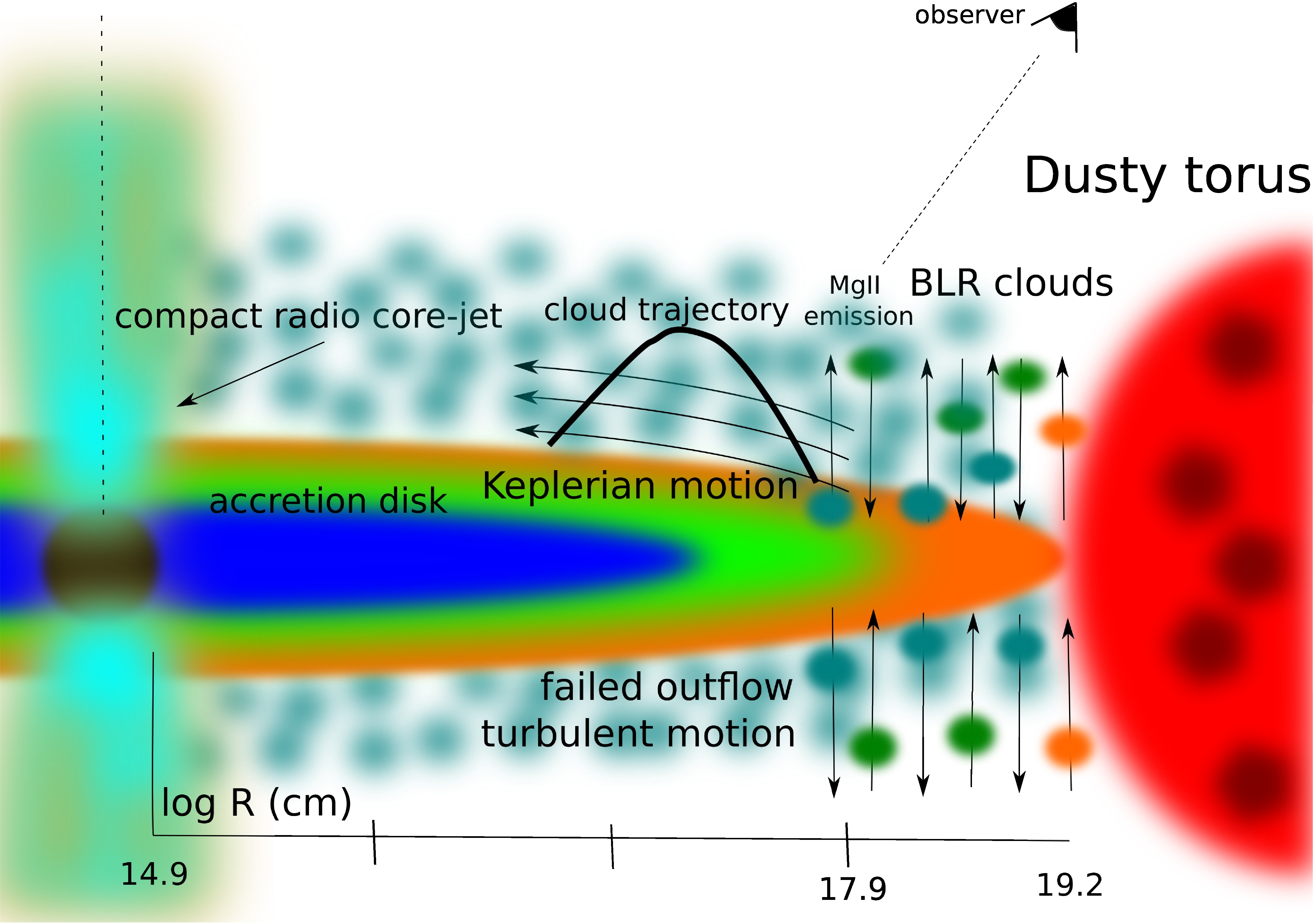
Figure 11: Illustration of the flattened distribution of the broad-line region clouds based on the MgII reverberation-mapping of the luminous intermediate-redshift quasar HE 0413-4031 ($z=1.38$). Adopted from Zajaček et al., 2020c [703].

The basic length-scale of the BLR region is given by Eq. (42), and it was only recently kinematically resolved out on sub-parsec scales using the Very Large Telescope Interferometer (VLTI) GRAVITY in the quasar 3C273 [272]. They reported a spatial offset of $0.03\,{\rm pc}$ between the red-shifted and blue-shifted photocenters of the broad Pa$\alpha$ emission line along the direction perpendicular to the jet. The detected velocity gradient implies the Keplerian rotation of the emitting gaseous material. The data are well-fitted by a thick disc of BLR cloudlets, which is in a Keplerian rotation around the black hole of $M_{\rm 3C273}\approx 3\times 10^{8}\,M_{\odot}$. The inferred BLR radius is 150 light days $\sim 0.126\,{\rm pc}$, which is consistent with the general Keplerian estimate for the comparable black hole mass in Eq. (42).

It was shown that the size of the BLR region is linked to the monochromatic luminosity and the BLR flux from a given emission line is mainly produced at a region with a specific combination of the gas density and the density of ionizing photons [38]. This locally optimally emitting cloud model (LOC) explains the observed variation of the BLR size with the monochromatic luminosity, which is also known as the BLR “breathing". The BLR “breathing" has been apparent from early reverberation mapping studies of broad Balmer emission lines [mainly H$\beta$ line centered at 4861Å ; 255, 357, 111, 174, 520, 44, 574, ; see the details below] that belong to recombination lines. The basic feature of the BLR breathing can observationally be described as follows. As the central ionizing luminosity increases, so does the BLR radius approximately as $R_{\rm BLR}\propto L^{1/2}$, since more distant BLR clouds are photoionized and produce a given BLR line. In relation to that, the width of the broad line decreases approximately as $\Delta v_{\rm BLR}\propto R_{\rm BLR}^{-1/2}\propto L^{-1/4}$, which holds under the assumption that the corresponding BLR emitting material is virialized. The LOC model is physically motivated in a sense that the line emission is given by the sum of the emission from individual clouds with different densities and distances from the central source of ionizing continuum. The whole system has an axisymmetric geometry [38]. The clouds are characterized by the distance distribution $f(r)\propto r^{\Gamma_{\rm r}}$ and the density distribution $g(n)\propto n^{\gamma_{\rm n}}$, where $\Gamma_{\rm r}\approx-1$ and $\gamma_{\rm n}\approx-1$ [38]. Then the line luminosity is given by,

$$L_{\rm line}\propto\iint_{R_{\rm in}}^{R_{\rm out}}\,r^{2}\,F(r)f(r)\,g(n)\,\mathrm{d}r\,\mathrm{d}n\,,$$ (44)

where $F(r)$ is an emission-line flux of a single cloud at the distance $r$. Using the integration scheme according to Eq. (44), the largest contribution comes from the clouds with the most efficient response to the continuum, i.e. clouds of a certain density range and at a distance where the ionizing photon flux reaches an optimum value. The LOC model implies that the overall BLR region is in fact much larger than the most emitting region that is observed.

The standard, powerful method to infer the length-scale of the BLR for a given source is the measurement of the time-delay between the observed variable continuum emission and the emission of one of the broad lines, typically Balmer lines (H$\alpha$, H$\beta$) or lines of some ions (MgII, CIV, CIII], FeII). This so-called reverberation mapping is possible since the variable continuum and line emission are significantly correlated, which in other words means that the ionizing continuum powered by the accretion disc is the main driver of the BLR variability and the BLR emission revealed in the form of emission lines is just the reprocessed UV/optical emission of the disc [83]. Mathematically, the reprocessing of the continuum flux by the BLR material located further away can be expressed via the so-called transfer function $\psi(\tau)$ [83, 534], which is a function of the rest-frame time-delay that depends on the distance of reprocessing clouds from the source $r$ as well as on the polar angle $\theta$ with respect to the line of sight,

$$\tau=\frac{r}{c}(1+\cos{\theta})\,.$$ (45)

The observer then sees the delayed line emission originating in all the clouds that are intersected by the iso-delay surface given by Eq. (45).

The transfer function $\psi(\tau)$ can then be determined as follows. Let $j_{\rm l}(t)$ be the emissivity of a broad line. In general, it responds in a non-linear way to the continuum flux changes $F_{\rm c}-\langle F_{\rm c}\rangle$ with respect to the mean value. If we approximate the line emissivity as a function of the continuum flux via the Taylor expansion around the mean value $\langle F_{\rm c}\rangle$, assuming the small changes of $F_{\rm c}$ above the mean value, we obtain,

$$j_{\rm l}(F_{\rm c})=j_{\rm l}(\langle F_{\rm c}\rangle)+\frac{\partial j_{\rm l}}{\partial F_{\rm c}}(F_{\rm c}-\langle F_{\rm c}\rangle)+\ldots\,.$$ (46)

The change in the line luminosity $\delta L_{\rm l}(t)$ can then be expressed as the convolution of the transfer function with the continuum line curve,

$$\delta L_{\rm l}(t)=\int_{0}^{\infty}\psi(\tau)\big{[}L_{\rm c}(t-\tau)-\langle L_{\rm c}\rangle\big{]}\mathrm{d}\tau\,,$$ (47)

where the transfer (or response) function is defined via the relation,

$$\psi(\tau)=c\int_{S}\frac{f(\mathbf{r})}{4\pi r^{2}}\frac{\partial j_{\rm l}}{\partial F_{\rm c}}\mathrm{d}A\,,$$ (48)

where the surface of integration is the isodelay surface for the time-delay $\tau$, as given by Eq. (45) and $f(\mathbf{r})$ is the local volume filling factor at the position $\mathbf{r}$ from the source. The determination of the transfer function $\psi(\tau)$, which is centered at the mean time-delay $\tau$, is generally time-consuming. This is related to the fact that to obtain $\psi(\tau)$ one needs to make an inversion of the convolution in Eq. (47), i.e. to perform the following Fourier transform

$$\psi(\tau)=\int e^{-i2\pi\nu\tau}\frac{\hat{L}_{\rm l}(\nu)}{\hat{L}_{\rm c}(\nu)}\mathrm{d}\nu\,,$$ (49)

where $\hat{L}_{\rm l}(\nu)$ and $\hat{L}_{\rm c}(\nu)$ are Fourier transforms of the line-emission and continuum light curves. To map out $\psi(\tau)$ with a sufficient precision, the Fourier-transforms of the light curves that are functions of $\propto\tau^{-1}$ need to be determined using the time-step smaller than $\Delta t<\tau/2$. In case the broad line is divided into several wavelength bins, in particular the line center and at least two line-wing regions, which correspond to different line-of-sight velocities $v_{\rm LOS}=v_{\rm orb}\sin{\theta}$ of the emitting gas, one can determine the transfer function $\psi(v_{\rm LOS},\tau)$ as a function of the line-of-sight velocity and the time delay, which is also referred to as the wavelength-resolved reverberation mapping.

The observed time-delay can be determined using the interpolated cross-correlation function (ICCF), its discrete version (DCF), $z$-transformed DCF (zDCF), damped random-walk modelling of the continuum emission using the JAVELIN module, the $\chi^{2}$ method, data regularity/randomness estimators (von Neuman, Bartels), see e.g. Zajaček et al., 2019b [702], Zajaček et al., 2020c [703], Rakshit, [554], Zajaček et al., [704] for the application of several methods and references therein. Once the time-delay was determined in the observer’s frame, it is straightforward to obtain the estimate of the rest-frame time-delay using the source redshift, $\tau_{\rm rest}=\tau_{\rm obs}/(1+z)$. For the mean distance of the BLR line-emitting material, we can simply use $R_{\rm BLR}=c\tau_{\rm rest}$.

From the series of spectra, one can obtain the length-scale of the BLR $R_{\rm BLR}$ as well as the line width, which serves as a proxy for the gas orbital velocity in type I AGN. Using the full width at half maximum (FWHM) of the broad line expressed in km/s, one can obtain the gas orbital velocity as $v_{\rm BLR}=f_{\rm c}v_{\rm FWHM}$, where the factor $f_{\rm c}$ depends on the BLR viewing angle, geometry, and the kinematics. Assuming that the BLR cloud motion is virialized, we can use the virial theorem given in Eq. (27) to obtain the virial black hole mass,

$$M_{\rm vir} =\frac{R_{\rm BLR}v_{\rm BLR}^{2}}{G}\,,\,$$

$$=f_{\rm c}^{2}\frac{c\tau_{\rm rest}v_{\rm FWHM}^{2}}{G}\,,$$

$$=f_{\rm vir}\frac{c\tau_{\rm rest}v_{\rm FWHM}^{2}}{G}\,,$$ (50)

where we have denoted $f_{\rm vir}=f_{\rm c}^{2}$, which is a so-called virial factor. It depends on the BLR geometry, kinematics as well as the viewing angle approximately in the following form [138, 426],

$$f_{\rm vir}=[4(\sin^{2}{\iota}+(H_{\rm BLR}/R_{\rm BLR})^{2})]^{-1}\,,$$ (51)

where $\iota$ is the viewing angle of the BLR plane with respect to the line of sight. In case $f_{\rm vir}$ depends only on the viewing angle, $f_{\rm vir}\approx(4\sin^{2}{\iota})^{-1}$, $f_{\rm vir}\approx 1$ for $\iota\approx 30^{\circ}$. However, fixing the virial factor to a single value of the order of unity, which is usually done in single-epoch spectroscopic mass determination [688], can introduce an error by a factor of $\sim 2-3$ in the virial black hole mass determination measurements [426]. By comparing the SMBH mass inferred from the spectral energy distribution fitting and the reverberation mapping Mejía-Restrepo et al., [426] found out that the virial factor is inversely proportional to the FWHM of broad lines, $f_{\rm vir}\propto\mathrm{FWHM}^{-1}$, which reflects the dependence on the BLR viewing angle or the effect of the radiation pressure on the BLR geometrical distribution.

Furthermore, it was found out that the size of the BLR or the rest-frame time delay are correlated with the monochromatic optical/UV continuum luminosity of the AGN [337, 336, 63, 158, 704, 693]. For instance, the H$\beta$ time delay is proportional to the $\sim 5000$ Å  luminosity, while MgII time lag is larger for larger $3000\,$Å  luminosity. This is a so-called radius-luminosity relation (RL), which has a simple power-law form, $\tau_{\rm rest}\propto L^{\alpha}$, where $\alpha\approx 0.5$ based on the simple photoionization theory. The power-law slope of $0.5$ stems from the definition of the ionization parameter of BLR clouds,

$$U=\frac{Q(H)}{4\pi R_{\rm BLR}^{2}cn(H)}\,,$$ (52)

where $R_{\rm BLR}$ is the cloud distance from the source of ionizing continuum, $n(H)$ is the cloud hydrogen density, and $Q(H)=\int_{\nu_{\rm i}}^{\infty}L_{\nu}/(h\nu)\mathrm{d}\nu$ is the hydrogen-ionizing photon flux in ${\rm cm^{-2}s^{-1}}$, where $\nu_{\rm i}$ is the lowest frequency of photons that can ionize the hydrogen atom. Under the assumption that $Un(H)$ is approximately constant for BLR clouds across different sources, we obtain $R_{\rm BLR}\propto Q^{1/2}(H)\propto L^{1/2}$.

In low-luminosity AGN, specifically the extremely low-luminous Galactic centre, $\sim$ 200 massive OB stars [523, 46] can provide essentially all the material that is partially accreted at the corresponding Bondi radius of $M_{\bullet}\simeq 4\times 10^{6}\,M_{\odot}$, but $>99\%$ forms an outflow that flattens the density profile of the accretion flow, $n\propto r^{-3/2+p}$, where $p\approx 1$ [674]. The mass-loading by stellar winds supplied by point sources or a spherical matter distribution was dealt in both semi-analytical and numerical approaches [553, 149, 245, 689, 562]. Steady-state 1D inflow-outflow solutions of the mass-loaded accretion flows contain a stagnation radius where the bulk velocity of the flow goes through zero Generozov et al., [see e.g. 245]. Inside the stagnation radius, inflow takes place, while outside it, the gas escapes the system. Under certain circumstances, both the inflow and the outflow reach supersonic velocities [689]. The stagnation radius is proportional to the gravitational parameter of the SMBH as for the Bondi radius, but it is inversely proportional to the square of the terminal wind velocity instead of the sound speed, under the assumption that stellar winds are faster than the stellar velocity dispersion, $v_{\rm w}>\sigma_{\star}$. Depending on the power-law slope $\Gamma$ of the stellar brightness profile, the stagnation radius can be expressed as [245],

$$R_{\rm stag} \approx\left(\frac{13+8\Gamma}{4+2\Gamma}-\frac{3\nu}{2+\Gamma}\right)\frac{GM_{\bullet}}{\nu v_{\rm w}^{2}}\,$$

$$\approx\begin{cases}15\,\left(\frac{M_{\bullet}}{2\times 10^{8}\,M_{\odot}}\right)\left(\frac{v_{\rm w}}{500\,{\rm km\,s^{-1}}}\right)^{-2}\,{\rm pc}&,\text{core\, ($\Gamma=0.1$)}\,,\\ 8\,\left(\frac{M_{\bullet}}{2\times 10^{8}\,M_{\odot}}\right)\left(\frac{v_{\rm w}}{500\,{\rm km\,s^{-1}}}\right)^{-2}\,{\rm pc}&,\text{cusp\, ($\Gamma=0.8$)}\,,\end{cases}$$ (53)

where we considered the core and the cusp stellar brightness distributions for the power-law slope $\Gamma$. The gas density slope $\nu\equiv-\mathrm{d}\rho/\mathrm{d}r|_{R_{\rm stag}}$ at the stagnation radius can be approximated using the stellar brightness slope $\nu\approx 1/6(4\Gamma+3)$. In general, the ratio of the stagnation radius to the Bondi radius is of the order of unity,

$$\frac{R_{\rm Stag}}{R_{\rm B}}\approx\frac{13+8\Gamma}{(2+\Gamma)(3+4\Gamma)}\,.$$ (54)

The basic length-scales inside the sphere of influence of the SMBH are depicted in Figure 12, where we assumed quasi-spherical distribution of stellar sources sources as well as the spherical distribution of hot plasma.

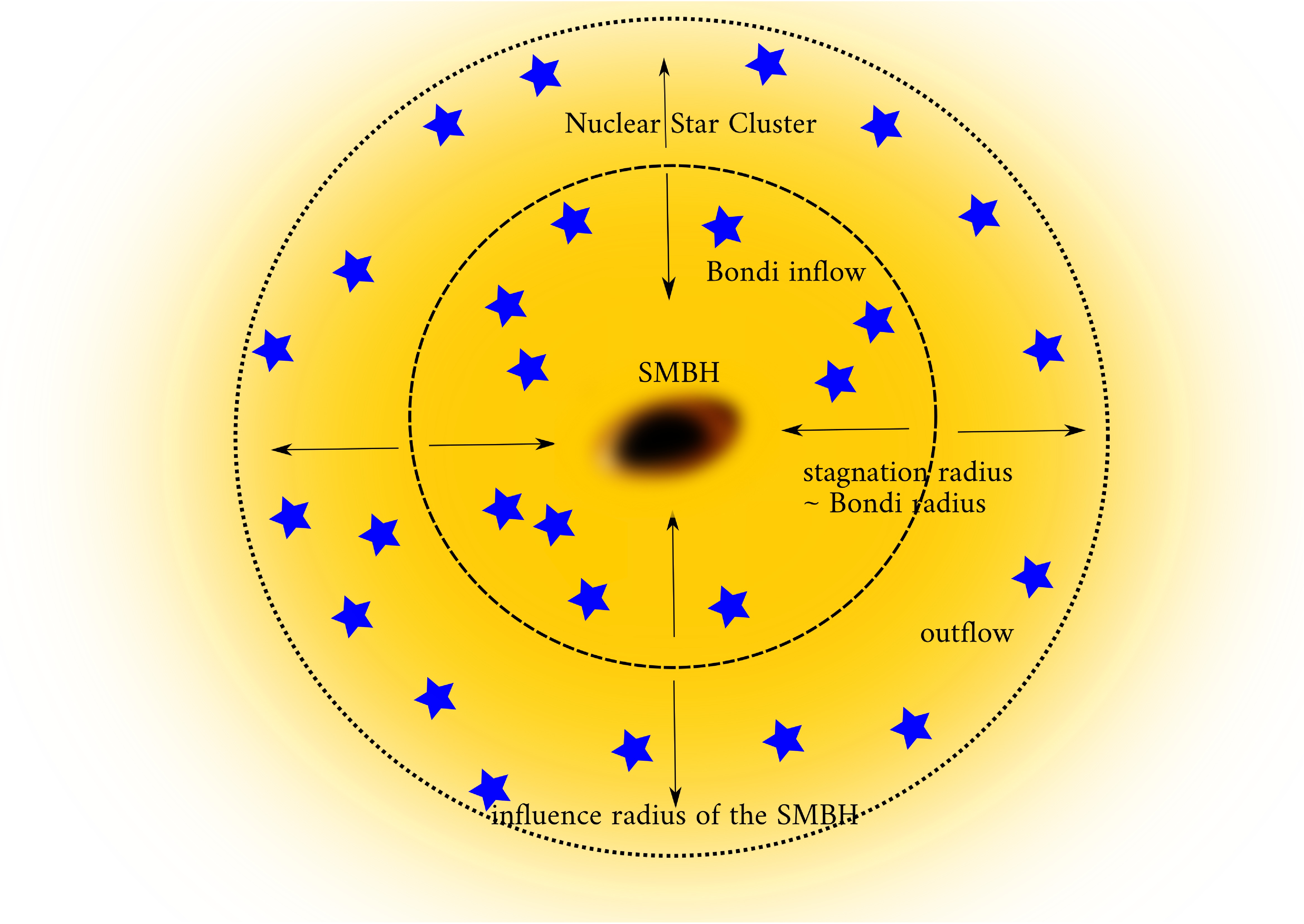
Figure 12: Illustration of the basic scales in the quasispherical Nuclear Star Cluster (NSC), inside the sphere of influence of the SMBH. Stellar outflows influence the hydrodynamics in such a way so that the hot flow develops a stagnation radius where its radial velocity reaches zero. Inside the stagnation radius, nearly radial Bondi flow can develop and power the accretion on the low-luminous SMBH, such as Sgr A*. Drawn not to the scale.

Extending the analysis above for AGN would require certain modifications, namely the extra radiation field (non-thermal continuum from the very centre and the thermal disk emission) and the gravitational influence of the disk and the dusty torus. In the AGN, there needs to be extra material available for the accretion apart from the stellar wind supply. For quasars, the accretion rate is of the order of $\dot{M}_{\rm acc}\approx 1\,M_{\odot}\,{\rm yr^{-1}}$, for Seyfert galaxies it is about two orders of magnitude smaller. In comparison, in the Galactic centre, based on the polarization measurements of sub-mm emission, the accretion rate is much smaller, $\dot{M}_{\rm acc}\approx 10^{-7}-10^{-9}\,M_{\odot}{\rm yr^{-1}}$ [412]. In general, the structure of the central parts of galaxies differs quite significantly between quasars and low-luminosity nuclei, depending thus on the accretion rate and thus the overall supply of the material.

Nevertheless, stars, stellar clusters and supernovae are expected to influence the circumnuclear medium in AGN and stars have been employed to explain some of the observables in the broad line region [532, 658].

Observational signatures of the broad line region

AGN show prominent emission lines in the UV as well as the optical part of the electromagnetic spectrum on the top of UV and optical non-stellar continuum. According to the full width at half maximum (FWHM), these lines are generally classified as broad (FWHM$\approx 1000-25000\,{\rm km\,s^{-1}}$) and narrow (FWHM$\approx 200-1000\,{\rm km\,s^{-1}}$), but there are AGN sources that do not exhibit any emission lines or only during a low-state of the central variable continuum source (in particular blazars, [624]). The unified model of AGN can generally explain the presence and the absence of broad emission lines in their spectra for type I and II AGN, respectively, depending on the inclination of the system with respect to the observer and hence the blocking of UV/optical photons by an optically and geometrically thick dusty torus that is clumpy, which leads to the disappearance of broad lines for type II AGN when observed in the total, unpolarized intensity (see e.g. [25, 24, 648]). Narrow-line components are mostly due to forbidden transitions, they are emitted by a low-density gas ($n\sim 10^{3}\,\rm cm^{-3}$), which is spatially extended and partially resolved for nearby AGN [62]. While the broad lines are dominantly caused by permitted transitions in the denser medium with the number density of $n>10^{8}\,{\rm cm^{-3}}$. Furthermore, narrow lines are often superposed on the broader component, which resulted in the subclassification of Seyfert galaxies into intermediate classes depending on the relative strength of the broad and narrow components (hereafter BC and NC, respectively; [506, 502, 503, 683]). BC emission lines respond to the continuum variation, but with a shorter time delay, which indicates that broad-line emitting region is photoionized and optically thick to ionizing continuum. On the other hand, NC emission lines do not show a correlated variation since they are emitted by a spatially extended region where the ionizing continuum is geometrically diluted and the recombination time scale is very long.

Broad lines led to the identification of quasars [585] and remain essential in studying accretion processes, outflows from the nuclear region as well as the effect of the central variable continuum source on the circumnuclear medium as well as the host galaxy as a whole. The AGN cover a large redshift range from the local sources such as M81 at $d=3.2\,{\rm Mpc}$ or the brightest AGN in the X-ray domain Cen-A [468] at $d=4.4\,{\rm Mpc}$ up to $z\approx 7.1$ (ULAS J1120+0641; [460]), at which the first quasars started to contribute to the reionization of the intergalactic medium. Therefore different broad lines from the rest-frame optical and UV part of the spectrum are suited for their monitoring in the observer-frame optical domain depending on the source redshift: HI H$\alpha$, $z=0.0-0.5$; H$\beta$, $z=0.0-1.0$; MgII$\lambda 2800$, $z=0.3-2.6$; CIII] $\lambda 1909$, $z=0.8-4.2$ (semi-forbidden line); CIV$\lambda 1549$, $z=1.2-5.4$; HI Ly$\alpha$, $z=1.9-7.2$ [624].

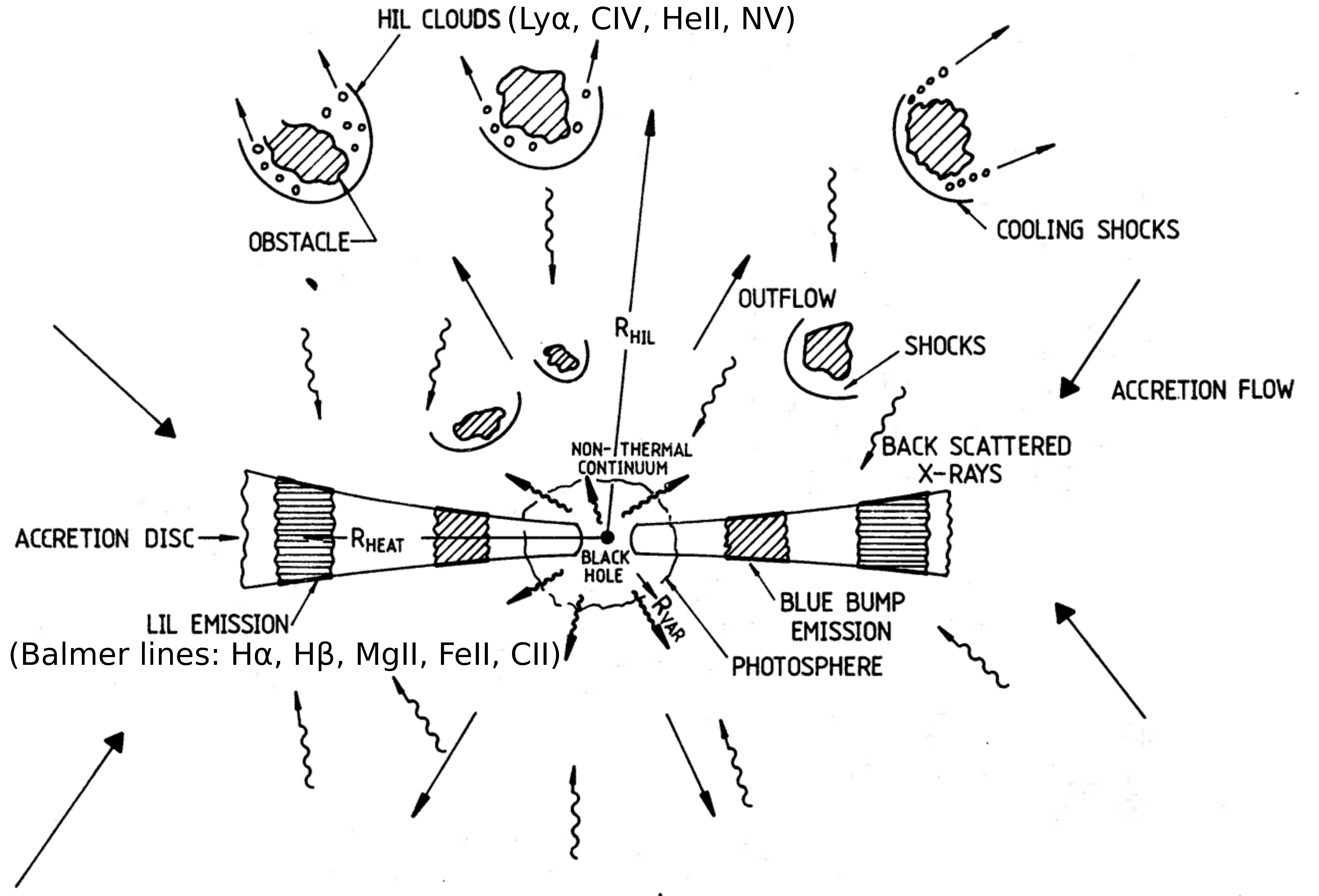
Figure 13: An illustration of the low- and high-ionization components of the Broad Line Region (BLR) in AGN (denoted as LIL and HIL). While the LIL component is mostly virialized and positioned close to the disc plane, the HIL part is associated with the nuclear outflows. The original illustration is from Collin-Souffrin et al., [141], where we added examples of both low-ionization lines used for the reverberation-mapping and high-ionization lines.

A two-component model was proposed for the BLR region [141] that consists of low- and high-ionization lines, see Figure 13 for the illustration. The emission lines that belong to the low-ionization lines (LIL, with an ionization potential $\lesssim$20 eV), such as most of Balmer lines as $H\beta$, CII $\lambda 1336$, and MgII$\lambda 2800$ and the pseudo-continuum of FeII, form in the mildly ionized, higher density regions $(n>10^{11}\,{\rm cm^{-3}})$ close to or directly in the extended parts of the accretion disc with no inflow/outflow signatures. However, when the accretion rate is close to the Eddington limit, low ionization lines show the presence of outflows (e.g. [478]). The high-ionization lines (HIL, with an ionization potential $\gtrsim$40 eV), such as Ly$\alpha$, CIV $\lambda 1549$, HeII $\lambda 1640$, and NV $\lambda 1240$, form in the highly ionized, lower density regions $(n<10^{10}\,{\rm cm^{-3}})$ associated with an outflow beyond the disc, but still close to the central black hole, as inferred from the reverberation mapping studies. Blueward asymmetries and blueshifted peaks with respect to the rest-frame of the HIL indicate the existence of disk winds in AGN [467, 243, 623]. Considering the general behavior of the LIL, observations indicate the coexistence of virial and radiation forces in the BLR. The disk wind model also supports the existence of the broad absorption outflows in the UV and X-ray domain of the AGN spectra, which are generally blueshifted [549, 610].

Around $1\%$ of the type-1 AGN show a double-peak profile mainly in the Balmer lines. Due to the variation in the peak profiles of months to years, this effect is due to a rotating disk [213], where the line-emission of the disk has a small optical depth and/or the line-emitting annulus of the disk is narrow [251, 233].

Formation and stability of BLR clouds

The BLR is generally envisaged as a collection of clouds with a certain geometrical distribution and a velocity field, which is determined mainly by the potential of the SMBH since the BLR clouds are located well inside its sphere of gravitational influence, see Eq. (43), as well as by radiation pressure of an accretion disc and potentially other effects, such as gas pressure gradient and magnetic field. Already early models of the BLR propose that its dynamics and ionized emission correspond to that of the clumpy, cloudy medium (see e.g. Netzer, [481]). The intercloud medium is of a lower density and higher ionization and therefore does not contribute significantly. The photoionization equilibrium is attained when the photoionization rate is balanced by the recombination rate, which can be expressed by an ionization parameter $U_{\rm ion}$,

$$U_{\rm ion}=\frac{Q_{\rm ion}(H)}{4\pi r^{2}cn_{\rm e}}\,,$$ (55)

which reflects the ratio of the density of hydrogen-ionizing photons and the electron density that stands for the recombination rate. The number of ionizing photons $Q_{\rm ion}(H)=\int_{\nu_{\rm i}}^{+\infty}(L_{\nu}/h\nu)\mathrm{d}\nu$ is obtained by integrating the ratio $L_{\nu}/h\nu$ over the photon spectrum that can ionize hydrogen and $L_{\nu}$ is the ionizing luminosity of the AGN. The BLR emission line strengths require the photoionization equilibrium at the temperature of $T\sim 10^{4}\,{\rm K}$ similar to plasma in HII regions and planetary nebulae [481, 624].

It has been recognized early on that the BLR region consists of two distinct components with a likely different origin [141]:

• the low-ionization line (LIL) component, revealed by lines with a low ionization potential (<20 eV), such as H$\beta$, MgII, and FeII, which does not reveal a significant inflow-outflow motion, and that likely forms in the denser region closer to the accretion disc,

• the high-ionization line (HIL) component, whose lines (e.g. Ly$\alpha$, HeII, CIV) with a higher ionization potential (>40 eV) exhibit an outflow motion revealed via blueward asymmetries and blueshifted line peaks, that forms in the lower-density, outflowing gas, but still close to the SMBH as revealed via the measured time-lags of HIL lines.

For an illustration of the LIL and HIL components of the BLR, see Fig. 13 and the corresponding more detailed discussion. In the following text, we focus on the formation mechanisms and the stability of the LIL component.

Rare detection of broad absorption features in type-I AGN (AGN with broad emission lines) suggests a flattened structure of the BLR. On the other hand, the clouds cannot be too close to the disc or within the disk since the covering factor of the irradiating continuum flux needs to be $\sim 30-50\%$ [357] to account for the observed significant correlation between the continuum and the broad-line emission. Therefore, the BLR clouds are more likely distributed in a torus-like or a ring-like geometry.

The BLR inner radius is set up by a specific formation mechanism, such as the dust formation within the disk that can lead to a dust-driven wind [155]. When such a wind gets high enough above the equatorial plane, the dust is exposed to intensive UV irradiation from the AGN and eventually destroyed. The dust-driven wind fails to further expand and the gas cloud drops back to the disk plane. This mechanism can well explain the appearance of the BLR clouds at the distance of roughly the same temperature around 1000 K in the accretion disk, as well as the turbulent velocity field due to the mixture of inflowing and outflowing components. The accretion disk self-shielding or the inner accretion disk wind can provide more shielding from the central irradiation, allowing the gas clouds to get further above the equatorial plane. This can explain the observed X-ray absorption by BLR clouds observed in intermediate AGN types [628].

The BLR outer radius can be considered to coincide with the inner radius of the dusty molecular torus – i.e. the dust sublimation radius, which can be estimated based on Nenkova et al., [480],

$$R_{\rm d}\simeq 0.4\left(\frac{L}{10^{45}\,{\rm erg\,s^{-1}}}\right)^{1/2}\left(\frac{T_{\rm sub}}{1500\,{\rm K}}\right)^{-2.6}\,{\rm pc}\,,$$ (56)

which is almost identical to Eq. (3) in terms of the normalization, but with a small difference of the power of the dust sublimation temperature $T_{\rm sub}$, i.e. $2.6$ instead of $2.8$, which stems from more detailed radiative transfer calculations of Nenkova et al., [480]. The mean rest-frame distance of the BLR is given by the measured time-delay between the continuum and the specific line-emission light curves, $R_{\rm BLR}\sim c\tau_{\rm BLR}$, where $\tau_{\rm BLR}$ depends on the specific line emission. It was revealed that there is a power-law relation between $\tau_{\rm BLR}$ and the monochromatic luminosity of the accretion disc, $L_{\rm mon}$, with the expected dependence $\tau_{\rm BLR}\propto L_{\rm mon}^{1/2}$ based on the constant photoionization parameter and the cloud density as we discussed in Subsection 1.4, see Eq. (52). This is a so-called radius-luminosity (RL) relation. For the broad H$\beta$ line, the RL relation is consistent with the square-root law with a scatter of $0.13$ dex for the initial sample, see Bentz et al., [63],

$$\log{\left(\frac{\tau_{H\beta}}{1\,{\rm lt-day}}\right)}=1.527^{+0.031}_{-0.031}+0.533^{+0.035}_{-0.033}\log{\left(\frac{L_{5100}}{10^{44}\,{\rm erg\,s^{-1}}}\right)}\,.$$ (57)

As the number of sources increased, especially including less variable and highly accreting sources, the scatter along the RL relation became more prominent. It was shown that the departure from the best-fit RL relation is correlated with the accretion rate, i.e. it tends to be larger for the high-accretion rate sources, see Martínez-Aldama et al., [413] and references therein. One of possible interpretations is that at higher accretion rates, the disc becomes geometrically thicker, i.e. it is a slim disc instead of a thin Shakura–Sunyaev type, and shields the radiation from its inner parts [673]. In this sense, the radiation field that the BLR clouds see is modified and generally anisotropic. In particular, the measured time-delay corresponds to a smaller luminosity and is thus effectively shorter [673].

The relevance of the RL relation lies in the fact that it is essential as a secondary black hole mass estimator using just a single spectrum, without the necessity to measure the BLR time delay for each source [376, 669, 424, 656], which is challenging to determine for fainter AGN towards higher redshifts. From Eq. 57, it is possible to determine the rest-frame time delay from the monochromatic luminosity and the line FWHM can be obtained from the same spectrum. The virial black hole mass can then be calculated from Eq. (50) under the assumption of a virial factor. In this way, the RL relation is crucial for studying black-hole mass evolution across the cosmic history [424]. While the RL relation for H$\beta$ line has been verified for $\sim 100$ sources [413], it is essential to test the dependency $\tau_{\rm BLR}\propto L_{\rm mon}^{\alpha}$ for other lines for which the correlation and the time delay is detected. In particular, it is of interest to compare the best-fit slopes $\alpha$ between different broad emission lines. Towards higher redshifts, MgII line moves into the optical bands and the reverberation mapping using MgII can be performed with optical monitoring telescopes. Czerny et al., [158] showed the RL relation also exists for MgII line, with the further confirmation by Zajaček et al., 2020c [703] using eleven sources, who showed that the scatter and the time-delay shortening for high-accreting sources is also present in the MgII RL relation. Using in total 69 sources, including the Sloan Digital Sky Survey Reverberation Mapping data [SDSS-RM; 299], Zajaček et al., [704] determined the intercept of $1.67\pm 0.05$ and the slope of $0.30\pm 0.05$ for the MgII RL relation, i.e. smaller than the canonical value, but with a large scatter of $\sim 0.30$ dex. In summary, the RL relation can be used for estimating the characteristic length-scale of the BLR region once the luminosity of the source is known.

The direct confirmation of the flattened structure of the BLR was provided by the first images of the BLR obtained using broad infrared lines resolved by the infrared Very Large Telescope Interferometer GRAVITY [265]. The flattened geometry and the velocity field is consistent with an orbiting gas bound to the central black hole, see in particular observations of 3C273 using broad Pa$\alpha$ line by Gravity Collaboration et al., 2018c [272], NGC3783 using broad Br$\gamma$ line by Gravity Collaboration et al., 2021b [270], and IRAS 09149-6206 analyzed using broad Br$\gamma$ line by Gravity Collaboration et al., 2020b [271]. For NGC3783, observations are consistent with the thick, rotating ring of clouds, whose radial distribution peaks close to the inner edge. The temperature of the BLR clouds is kept at $\sim 10\,000-20\,000\,{\rm K}$ due to the atomic-transition, radiative heating/cooling in the partially ionized plasma, independent of the ionizing flux across different sources. The very intense irradiation by a hard ionizing continuum of the AGN leads to the complete ionization and the heating/cooling balance is established at $\sim 10^{7}\,{\rm K}$ due to Compton heating/cooling. In the plasma irradiated by an AGN, thermal instability is expected to develop and the partially ionized clouds having $\sim 10^{4}\,{\rm K}$ are in an approximate pressure equilibrium with the hot and diluted phase at $\sim 10^{7}\,{\rm K}$ [367], i.e. the clouds are confined by a hot intercloud medium. At this two-phase balance, the evaporation timescale of the colder plasma due to thermal conduction is comparable to the timescale, during which the hot phase cools down and condenses onto clouds, see also the discussion and the estimates of the evaporation/condensation timescales below. Hence, the lifetime and the stability of BLR clouds is difficult to determine, but supposedly it is of the order of the orbital timescale or its fraction as we will demonstrate based on the evaporation/condensation as well as tidal timescales.

For the estimate of the basic timescales, we assume the column density of the BLR gas of $N_{\rm cl}\sim 10^{24}\,{\rm cm^{-2}}$ and the volume number density of $n_{\rm cl}\sim 10^{12}\,{\rm cm^{-3}}$, from which the basic length-scale or a cloud radius can be estimated as $R_{\rm cl}\sim N_{\rm cl}/n_{\rm cl}\sim 10^{12}\,{\rm cm}$ [see e.g. 153, 10]. The average mass of BLR clouds is thus of the order of $M_{\rm cl}\sim 4/3\pi R_{\rm cl}^{3}m_{\rm p}n_{\rm cl}\sim 7.0\times 10^{24}\,{\rm g}\sim 7.5\,M_{\rm Ceres}$, which is comparable to the mass of a large asteroid (a few times of the mass of Ceres). The basic intrinsic dynamical timescale of BLR clouds is given by the perturbation propagation timescale, which can be estimated as the ratio of the cloud radius to the sound speed inside the cloud, where we assume the isothermal sound speed for $T_{\rm cl}\sim 10^{4}\,{\rm K}$,

$$\tau_{\rm dyn} =\frac{R_{\rm cl}}{c_{\rm cl}}\,$$

$$\simeq 13\,\left(\frac{R_{\rm cl}}{10^{12}\,{\rm cm}}\right)\left(\frac{T_{\rm cl}}{10^{4}\,{\rm K}}\right)^{-1/2}\text{days}\,.$$ (58)

Due to the coexistence of two fluids with different densities in the BLR region (hot diluted intercloud medium and colder, denser BLR clouds) as well as the likely existence of the velocity shear $v_{\rm shear}$ between the two phases, the BLR cloud will be significantly perturbed or disrupting on a crushing timescale that is equal to a shock-propagating timescale [see e.g. 419],

$$\tau_{\rm crush} =\frac{R_{\rm cl}}{v_{\rm shear}}\sqrt{r_{\rho}}\,$$

$$=3.7\,\left(\frac{R_{\rm cl}}{10^{12}\,{\rm cm}}\right)\left(\frac{v_{\rm shear}}{1000\,{\rm km\,s^{-1}}}\right)^{-1}\left(\frac{r_{\rho}}{10^{3}}\right)^{1/2}\text{days}\,,$$ (59)

where $r_{\rho}=n_{\rm cl}/n_{\rm h}$ denotes the density ratio between the cloud and the hot intercloud medium. Assuming the pressure equilibrium and the confinement of the BLR clouds by hot diluted intercloud medium, we obtain $r_{\rho}\sim n_{\rm cl}/n_{\rm h}=T_{\rm h}/T_{\rm cl}\sim 10^{3}$. The development of the Kelvin-Helmholtz instability due to the velocity shear as well as the Rayleigh-Taylor instability due to the centrifugal acceleration in the shock propagating through the cloud occurs on timescales comparable to the crushing timescale expressed by Eq. (59). This timescale related to the hydrodynamical instabilities would imply the BLR cloud lifetime of at least a few days.

However, the lifetime of clouds is plausibly longer than indicated by Eq. (59) due to stabilisation mechanisms that prevent the quick development of large-scale hydrodynamical instabilities. In the BLR region, these mechanisms contribute:

• slow cooling or warm circumnuclear medium, see e.g. discussion in Decin et al., [173],

• ionizing radiation from external sources, in particular X-ray/UV emission of the inner accretion disc [277], which heats up the surrounding gas content, which is linked to point (i),

• circumnuclear magnetic field [652].

In the BLR region, all the conditions (i), (ii), and (iii) are present to a smaller or a larger extent. The ionizing radiation, which keeps the circumnuclear medium warm, increases the thermal gas pressure that suppresses the growth of Rayleigh-Taylor fingers and other instabilities in BLR clouds. This is confirmed by numerical hydrodynamical simulations. In Vieser and Hensler, [657], authors present dynamical models of cold clouds moving through the hot interstellar medium. Such a set-up is common in several astrophysical settings, including cooling flows in galactic halos, star-forming regions where cold molecular clouds are surrounded by young massive stars, and it is also applicable to the BLR region in the gravitational influence of the SMBH. They demonstrate that heat conduction smooths steep temperature as well as density gradients at the cloud boundary since the heat conduction timescale is shorter than the cooling timescale. As a result, there is a decrease in the shearing velocity between the cloud surface and the hot medium. According to Eq. (59), this results in the prolongation of the crushing timescale as well as the timescale for the development of the Kelvin-Helmholtz instability and colder BLR clouds can survive the passage through the hot intercloud medium, at least for a significant fraction of their orbital period.

The BLR region, as described earlier, can be envisaged as a multiphase medium similar to other astrophysical set-ups [423]. It consists of at least two phases – cold, dense BLR clouds and hot, diluted intercloud medium – that are approximately in pressure equilibrium since the circumnuclear medium is externally heated by an AGN. The BLR clouds cool down radiatively via atomic transitions in the partially ionized plasma, while the hot, diluted intercloud medium that is fully ionized cools down via Compton cooling. This way the two phases can stay in pressure equilibrium with BLR clouds having $\sim(10-20)\times 10^{3}\,{\rm K}$ and the intercloud medium with $\sim 10^{7}\,K$ [367]. The BLR region is certainly not stationary but dynamic. There is a certain velocity shear between the clouds and the hot intercloud medium. The basic estimate of the velocity difference is given by the broad line FWHM of a few $1000\,{\rm km\,s^{-1}}$. If we consider the value of $v_{\rm FWHM}=5000\,{\rm km\,s^{-1}}$ for a circular velocity, this is associated with the characteristic BLR radius of

$$r_{\rm BLR} =\frac{GM_{\bullet}}{f_{\rm vir}v_{\rm FWHM}^{2}}\,$$

$$=0.017\left(\frac{M_{\bullet}}{10^{8}\,M_{\odot}}\right)\left(\frac{v_{\rm FWHM}}{5000\,{\rm km\,s^{-1}}}\right)^{-2}\left(\frac{f_{\rm vir}}{1}\right)^{-1}\,{\rm pc}\,.$$ (60)

The BLR distance can also be expressed in terms of gravitational radii,

$$\frac{r_{\rm BLR}}{r_{\rm g}} =f_{\rm vir}^{-1}\left(\frac{c}{v_{\rm FWHM}}\right)^{2}\,$$

$$=3600f_{\rm vir}^{-1}\left(\frac{v_{\rm FWHM}}{5000\,{\rm km\,s^{-1}}}\right)^{-2}\,.$$ (61)

Since according to Mejía-Restrepo et al., [426] the virial factor $f_{\rm vir}$ is inversely proportional to the line FWHM, the dependence of $r_{\rm BLR}/r_{\rm g}$ on $v_{\rm FWHM}$ is expected to be formally weaker. However, for the broad component of H$\beta$ line, the virial factor dependency on the line FWHM is [426],

$$f_{\rm vir}^{H\beta}=\left(\frac{v_{\rm FWHM}}{4550\pm 1000\,{\rm km\,s^{-1}}}\right)^{-1.17\pm 0.11}\,,$$ (62)

which for FWHM close to $5000\,{\rm km\,s^{-1}}$ yields $f_{\rm vir}\approx 1$. We note that the typical BLR region length-scale given by Eqs. (60) and (61) is comparable to the S cluster size in the Galactic center [194, 195], see also Subsection 1.5 for further details.

The orbital timescale can be expressed as, under the assumption of a circular motion,

$$\tau_{\rm orb} =\frac{2\pi GM_{\bullet}}{v_{\rm FWHM}^{3}}\,$$

$$=21.1\left(\frac{M_{\bullet}}{10^{8}\,M_{\odot}}\right)\left(\frac{v_{\rm FWHM}}{5000\,{\rm km\,s^{-1}}}\right)^{-3}\,{\rm yr}\,.$$ (63)

The relative velocity of BLR clouds with respect to the intercloud medium $v_{\rm rel}$ is essentially between zero (clouds comoving with the dynamical hot medium) and $v_{\rm FWHM}$ (the hot medium is stationary). In case we assume the stationary hot medium, the BLR clouds move supersonically, i.e. $M=v_{\rm rel}/c_{\rm s}>1$, within the radius,

$$r_{M>1} <\frac{GM_{\bullet}\mu m_{\rm H}}{k_{\rm B}T_{\rm h}}\,$$

$$<2.6\,\left(\frac{M_{\bullet}}{10^{8}\,M_{\odot}}\right)\left(\frac{T_{\rm h}}{10^{7}\,{\rm K}}\right)^{-1}{\rm pc}\,,$$ (64)

which is essentially the whole BLR region, since the light-travel time in the rest frame for the maximum $r_{M>1}$ is $\tau_{c}=r_{M>1}/c\sim 3100$ days, which according to the radius-luminosity relation for the broad H$\beta$ line [63] would correspond to the very large monochromatic luminosity at 5100Å,.

$$\log\left(\frac{\tau}{1\,\text{lt-day}}\right) =1.527^{+0.031}_{-0.031}+0.533^{+0.035}_{-0.033}\log{\left(\frac{L_{5100}}{10^{44}\,{\rm erg\,s^{-1}}}\right)}\,$$

$$L_{5100} =10^{44+(\log{\tau_{\rm BLR}}-1.527)/0.533}\,{\rm erg\,s^{-1}}=10^{47.69\,{\rm erg\,s^{-1}}}\,.$$ (65)

The bolometric luminosity can be estimated from $L_{5100}$ using the bolometric correction, $L_{\rm bol}=\text{BC}\times L_{5100}$. According to Netzer, [484], the bolometric correction factor is a power-law function of the observed luminosity based on thin-disk calculations and X-ray properties of AGN,

$$\text{BC}=40\times\left(\frac{L_{5100}}{10^{42}\,{\rm erg\,s^{-1}}}\right)^{-0.2}\approx 2.9\,,$$ (66)

which is estimated for $L_{5100}=10^{47.69}\,{\rm erg\,s^{-1}}$. The bolometric luminosity then is $L_{\rm bol}=2.9\times 10^{47.69}\,{\rm erg\,s^{-1}}=10^{48.15}\,{\rm erg\,s^{-1}}$. The Eddington ratio can be estimated using Eq. (22),

$$\lambda_{\rm Edd}=\frac{L_{\rm bol}}{L_{\rm Edd}}\approx 112\,,$$ (67)

which is two orders of magnitude above the Eddington limit. In this sense, the limitation for the supersonic motion of BLR clouds, expressed by the relation (64), is met by a majority of AGN unless the hot intercloud is dynamic and partially comoving with the BLR clouds.

The shock propagates through the BLR cloud on the dynamical timescale, see Eq. (58), which is much shorter than the orbital timescale. Therefore the BLR cloud is shaped by stripping off the material that is located at the cloud-medium border, which results in the formation of the tail behind the denser head. This is also consistent with the detection of comet-shaped absorbers of the X-ray emission along the line of sight [403].

Since BLR clouds are confined by the hot intercloud medium, their evolution is affected strongly by the heat conduction. One can adopt in the first approximation the results of Cowie and McKee, [146], who studied the effect of heat conduction on spherical clouds embedded in hot plasma. In the diffusion approximation, the heat flux due to the heat conduction can be expressed as [657],

$$\mathbf{q_{diff}}=-\kappa_{\rm h}\mathbf{\nabla T}\,,$$ (68)

where the conductivity of the hot phase can be calculated as

$$\kappa_{\rm h}=\frac{1.84\times 10^{-5}T_{\rm h}^{5/2}}{\ln{\Psi}}\,{\rm erg\,s^{-1}K^{-1}cm^{-1}}\,,$$ (69)

where the Coulomb logarithm can be estimated as follows,

$$\ln{\Psi}=29.7+\ln{\left(\frac{T_{\rm e,6}}{\sqrt{n_{\rm e}}}\right)}\,,$$ (70)

where the electron density $n_{\rm e}$ is expressed in ${\rm cm^{-3}}$ and the electron temperature $T_{\rm e,6}$ is scaled to $10^{6}\,{\rm K}$.

Cowie and McKee, [146] derive a classical mass-loss rate due to heat conduction, in other words the evaporation rate,

$$\dot{m}_{\rm evap}=-\frac{16\pi\mu m_{\rm p}\kappa_{\rm h}R_{\rm cl}}{25k_{\rm B}}\,,$$ (71)

from which we can derive the evaporation timescale under the assumption of a constant cloud density, $m_{\rm cl}=4/3\pi R_{\rm cl}^{3}\rho_{\rm cl}$. Then the evaporation rate can also be expressed as $\dot{m}_{\rm evap}=4\pi R_{\rm cl}^{2}\dot{R}_{\rm cl}\mu n_{\rm cl}m_{\rm p}$. After plugging in Eq. (71), specifically on the left side, we obtain the expression for the evaporation timescale,

$$\tau_{\rm evap}=\frac{25k_{\rm B}n_{\rm cl}R_{\rm cl}^{2}}{8\kappa_{\rm h}}\,,$$ (72)

which depends on the cloud density, a square of its radius, and the temperature as well as the density of the surrounding hot medium. The conductivity for the hot medium is $\kappa_{\rm h}\approx 2.69\times 10^{11}\,{\rm erg\,s^{-1}\,K^{-1}\,cm^{-1}}$ under the assumption of the pressure equilibrium. Then the evaporation timescale of the BLR clouds can be estimated as follows,

$$\tau_{\rm evap}\simeq 51\,\left(\frac{n_{\rm cl}}{10^{12}\,{\rm cm^{-3}}}\right)\left(\frac{R_{\rm cl}}{10^{12}\,{\rm cm}}\right)^{2}\left(\frac{\kappa_{\rm h}}{2.69\times 10^{11}\,{\rm erg\,s^{-1}\,K^{-1}\,cm^{-1}}}\right)^{-1}\,{\rm yr}\,,$$ (73)

which is significantly larger than the hydrodynamical crushing timescale that is of the order of days, see Eq. (59).

The quasi-Keplerian motion of clouds in the potential of the SMBH can lead to the formation of broad emission lines with the FWHM of a few $1000\,{\rm km\,s^{-1}}$. The smooth line profile implies the high abundance of such dense clouds. The physical origin of the BLR line-emitting gas has remained largely unknown despite a large number of theoretical, observational, and computational studies. The BLR clumps may generally be formed in the inflow, in-situ in the disc via the gravitational instability, as a part of the irradiated accretion disk surface, or in the outflow. Reverberation mapping measurements imply that the Keplerian motion dominates but inflow or outflow signatures are also seen [275]. A more complicated picture involving all of these processes is also plausible [672, 670]. These scenarios are separately discussed below:

• Inflow models. Accretion onto the central black hole can, perhaps partially, proceed in the form of the BLR infall. Circumnuclear material/interstellar medium contains colder clouds embedded in a hotter intercloud medium. Colder material is more likely to accrete since its thermal velocity of gas particles is much lower that the escape velocity, and the infall will happen in the absence of the angular momentum barrier. Numerical simulations of the multi-phase medium show the infall of the cold clouds and the outflow of the hot X-ray emitting gas in the gravitational field [42, 209]. Convincing observational arguments for the inflow has been found by Hu et al., [304], and the consequences of this discovery to the BLR structure were discussed by Ferland et al., [230]. Since the force multiplier in the Fe II emitting region is very large, the infall is possible only if most of the clouds are actually shielded from the central source. We thus observe predominantly non-irradiated faces of the optically thick clouds, and this solves the long-standing problem of modelling Fe II to H$\beta$ ratio. On the other hand, observational determination of Fe II shifts is very complex and the shift claim might still be the artefact of the data analysis method [92]. The analysis of CIV line emission in NGC 5548 has indicated a large 2D or 3D random motion on the top of the radial infall, see [182]. In the context of inflow models, Elvis, 2017b [210] presented the model of the “quasar rain”, which involves a hot disk outflow, from which colder clumps can condense via the thermal instability [367]. These heavier and cold clumps than fall back towards the disk since they are not supported enough by the radiation pressure.

• In-situ cloud formation via gravitational instability – affect of the nuclear star cluster. AGN typically host massive and extended accretion disks that at larger distances are gravitational unstable due to the decreasing temperature and the increasing surface density. Hence, eventually the Toomre stability criterion drops below one and the disk fragments. At intermediate scales it can be supported against fragmentation by the turbulence, spiral waves or the magnetic field. The fragmenting self-gravitating disks have extensively been studied by several authors, see Collin and Zahn, [139], Collin and Zahn, [140] and references therein. More recently, Wang et al., [672] studied the complex processes taking place in the fragmenting star-forming AGN disks. In particular, supernova explosions lead to the ejection of gas above the disk plane. They can also contribute to the high, supersolar metallicity observed in quasars. There can generally be several cycles of BLR formation depending on starburst phases [670]. In the broader text, once the nuclear star cluster has formed and a fraction of stars has evolved over the billions of years, the stars as such could give rise to the BLR clouds. Alexander and Netzer, [16] and Alexander, [15] proposed the “bloated-stars” model where the broad lines could be produced by the collective emission of the extended envelopes of several $10^{4}$ stars located deep inside the sphere of influence of the SMBH. This model has, however, failed to explain some of the BLR characteristics, e.g. line profiles and the flattened geometry now detected by the GRAVITY instrument. For the evolved stellar population, we expect the orbital randomization by stellar resonant and non-resonant relaxation processes over the course of billions of years.

• Irradiated disk surface. In the context of the HIL and LIL components of the BLR [141], some LILs could be formed within the accretion disk on its surface since their velocity field is mainly given by the orbital Keplerian component. This is mainly the case of double-peak low-ionization lines [67, 212]. The velocity field of BLR clouds has the orbital Keplerian component as well as the turbulent component [353], which becomes more prominent for high-Eddington sources. The double-peak sources are generally associated with lower Eddington sources, where the orbital velocity component is dominant. From stationary models of the BLR associated with the accretion disk, Baskin and Laor, [48] showed the formation of the puffed-up stationary dusty atmosphere or rather “dust-inflated accretion disk" within the range where the dust opacity dominates. Nayakshin, [477] proposed that the accretion disc warping and precession due to an axisymmetric potential created by the previously formed stellar disk can be held responsible for lifting off some material above the original disk plane. This material can then obscure the AGN and contribute to the inclination-dependent emission of AGN.

• Outflow models. Outflow scenario is the most frequently adopted hypothesis, since a strong blueshift seen in high ionization UV lines, like for example CIV, is observed in numerous quasars [e.g. 103]. This outflow has been interpreted as an accretion disk wind Murray et al., [467], or bi-conical ejection along the symmetry axis [718]. The bi-conical structure was motivated by observations of the elongated Narrow Line Region (NLR), well seen for example in [OIII] emission, and the NLR has been hypothesized to be the extension of the outflowing BLR, see e.g. [98].

  The common prediction of the outflow models of the BLR is that the broad lines are present only as long as the classical cold accretion disk extends all the way to the BLR launching radius or rather the range of radii. In other words, the BLR lines are present only as long as the Big Blue Bump is present. For sources with the low Eddington ratio, such as also true Seyfert 2 galaxies (no broad lines, no obscuration), the broad lines disappear. This is also the case of low-luminosity Sgr A* and M87 where the accretion flow is represented by hot Advection-Dominated Accretion Flow or ADAF, see Yuan and Narayan, [694] for a review. Hot flows are accompanied by radially dependent outflows but these are fully ionized and not capable of producing broad lines. However, for at least one candidate true Seyfert 2 (NGC3147) with a low accretion rate of $\lambda_{\rm Edd}\sim 10^{-4}$, a double peak broad H$\alpha$ with the base width of as much as $\sim 27\,000\,{\rm km\,s^{-1}}$ was detected, see Bianchi et al., [67]. This finding to some extent questions the existence of true Seyfert 2 sources and the presence of the classical cold disc below $\sim 100$ gravitation radii for such low accretion rates is also beyond theoretical expectations. Below we list basic outflow models that are distinguished based on the driving force of the outflow: magnetically driven, thermally driven, and radiation-pressure driven winds. For a general overview of the disc-outflow mechanisms, see also Proga, [548] and Czerny, [153]. The formation, structure, and the evolution of the outflow is generally given by the equation of radiation magnetohydrodynamics [548]

  $$\rho\frac{\mathrm{D\mathbf{v}}}{\mathrm{D}t}+\rho\Phi=-\nabla P+\frac{1}{4\pi}(\nabla\times\mathbf{B})\times\mathbf{B}+\rho\mathbf{F}_{\rm rad}\,,$$ (74)

  where $\rho$, $\mathbf{v}$, and $P$ are the fluid density, velocity, and pressure. Furthermore, $\Phi$ denotes the gravitational potential, $\mathbf{B}$ stands for the magnetic field, and $\mathbf{F}_{\rm rad}$ is the radiation force per unit mass. To generate outflow, at least some of the terms on the right need to overcome the gravitational force, which can lead to the true outflow (escaping gas) or also a failed wind, for which some of the material returns back to the accretion disk. The mechanisms to generate the outflow are represented on the right-hand side: (a) the gas pressure gradient, (b) Lorentz force, and (c) the radiation-pressure force due to the radiation-pressure gradient. We discuss these mechanisms in more detail below.

  1. Thermally driven winds. Spontaneous thermal outflows can be initiated when the outer parts of the disk are heated to approximately the virial temperature. The virial temperature can be derived assuming the virial equilibrium, see Eq. (27), for the rotating gas with the thermal kinetic energy of $K_{\rm therm}=3/2Nk_{\rm B}T_{\rm vir}$, where we assumed the ideal monoatomic gas with $N=M_{\rm gas}/(\mu m_{\rm p})$ particles. Then the virial temperature can be approximated as,

     $$T_{\rm vir}\approx\frac{GM_{\bullet}\mu m_{\rm p}}{3k_{\rm B}r}=\frac{\mu m_{\rm p}}{3k_{\rm B}}v_{\rm gas}^{2}=\frac{\mu m_{\rm p}c^{2}}{3k_{\rm B}\hat{r}}\,,$$ (75)

     where $\hat{r}$ is expressed in gravitational radii. For $\hat{r}=10^{4}$, we obtain $T_{\rm vir}\sim 1.8\times 10^{8}\,{\rm K}$ or $k_{\rm B}T_{\rm vir}\sim 16\,{\rm keV}$, which corresponds to X-ray emitting plasma. The colder outer parts are heated by the warmer inner parts of the disc, mainly by X-ray irradiation. Specifically the Compton heating can bring the diluted cooler gas in the upper parts of the disc to the inverse Compton limit of $\sim 10^{8}\,{\rm K}$, see Begelman et al., [56] and Begelman and McKee, [55] for details. This balance is achieved by the Compton heating by hard photons and inverse Compton cooling by softer photons. In addition to the inverse Compton heating/cooling balance, a viscous dissipation close to the disk surface could be another source of heating [161]. Depending on whether the gas thermal speed exceeds the local escape speed from the disc, which is a function of radius, two solutions are possible – in case the escape speed is not exceeded, which is more likely in the inner disk parts with large escape velocities, a stationary puffed-up hot atmosphere forms above the disc (corona). In the opposite case, a thermally-driven wind is launched when the thermal gas speed exceeds the escape velocity, which is more likely in the outer disk parts. This wind is almost fully ionized and hence it is not efficient in producing lines. In some cases, if launched from the outer BLR or the dusty torus, it could be responsible for the observed low-velocity intervening warm absorbers, see Chelouche and Netzer, [127]. Thermally driven winds operate at high temperatures of $\sim 10^{7}-10^{8}\,{\rm K}$; for lower temperatures, the other terms in Eq. (74) dominate.

  2. Magnetically driven winds. In case the accretion disc is threaded by a large scale magnetic field with a significant poloidal component, a magnetically-driven wind can be launched via the magneto-centrifugal force [84]. For this model to work, the magnetic field needs to be transported inwards from the circumnuclear medium further out. Models of magnetically-driven winds predict the concave shape of flow lines and the gas escape speeds can achieve large velocities. The magnetically driven wind is also employed to explain the high-ionization UltraFast Outflows (UFOs) that are detected as absorption features in the X-ray spectra [238]. Fukumura et al., [238] constrain from the X-ray spectra the launching radius of UFOs at $\sim 200\,r_{\rm ISCO}$, where $r_{\rm ISCO}$ is the innermost stable circular orbit.

  3. Radiation-pressure driven winds. There are two potential sources of the opacity that we discuss further below – (i) absorption lines of various ionized species in the gas, for which the force multiplier $M$ that is introduced as the ratio of the total radiation pressure to the radiation pressure attributed to the Thomson scattering, can reach values of a few hundred, and (ii) the dust opacity, which is relevant for the distance where the disk temperature drops below the dust sublimation temperature and the dust can coexist with the gas. Case (i) – line-driven wind– is also responsible for driving fast and diluted stellar winds of hot OB stars, which is also known as the CAK theory or Castor–Abbott–Klein, see Castor et al., [119], while case (ii) – dust-driven wind– is relevant for slower and more massive outflows of late-type evolved stars, see Sedlmayr and Dominik, [592] for a review.

     

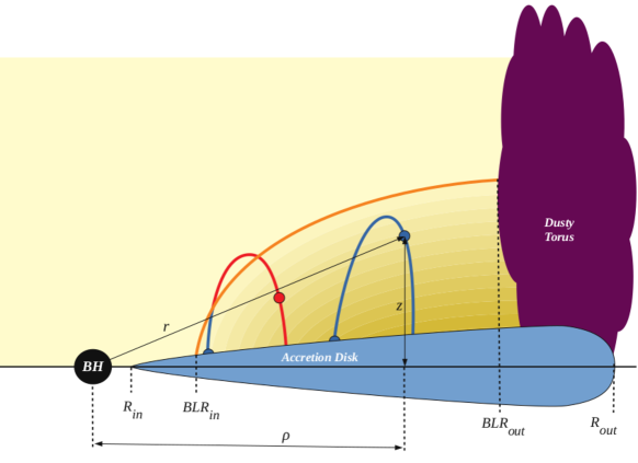
     Figure 14: The illustration of the Failed Radiatively Driven Dusty Outflow or FRADO model. In the disk zone where dust can form, i.e. where the effective disk temperature drops below the dust sublimation temperature, the dust opacity is high enough so that gaseous-dusty clumps are lifted off the disk plane due to the scattering of disk photons on dust grains. Once these BLR clouds are directly irradiated by external UV and X-ray photons, dust evaporates and clouds fall back to the disk since they are not supported by radiation pressure anymore. The dominant velocity component of the FRADO clouds is still orbital, i.e. Keplerian, but there is also an extra turbulent component due to the outflow-inflow of the BLR clouds. See also Czerny and Hryniewicz, [155] and Naddaf et al., [470] for details.

     

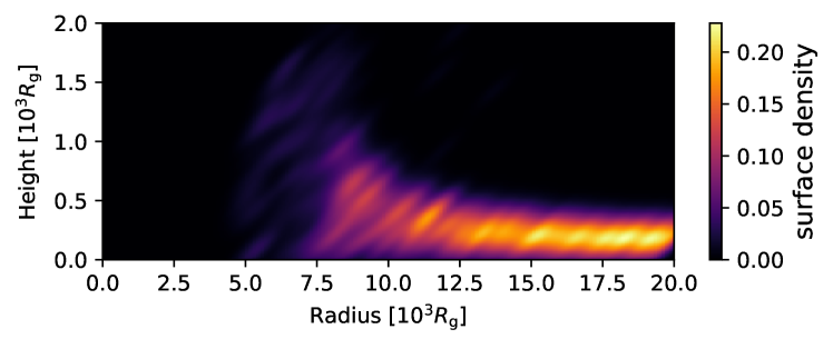
     Figure 15: The instantaneous surface-density distribution of the BLR clouds based on the dynamical calculations of the FRADO model, see Naddaf et al., [470] for details.

     Line-driven winds. The CAK-like mechanism was first applied to the AGN winds by Murray et al., [467]. In the follow-up paper by Chiang and Murray, [128], line profiles were calculated – both double-peak and single-peak lines could be produced by line-driven disk outflows. The inclusion of the large radial shear in the line-driven wind was necessary to reproduce the single-peak line-profile as well as the response (transfer) function of lines consistent with observations, including their red- and blue-wing responses, see also Murray and Chiang, [466]. Murray and Chiang, [465] also applied the disk wind driven by UV resonance lines to interpret broad absorption features in spectra. In recent years, there has been a large progress in hydrodynamical models of AGN winds. Waters et al., [675] used these simulations to calculate echo images, line profiles and response functions of BLR lines for different viewing angles. The wind hydrodynamics and the ionization state were not calculated simultaneously, instead the radiative transfer was performed a posteriori. A general consistency is found with observations as well as previous BLR model calculations. Previously, Proga et al., [550] and Proga and Kallman, [549] found from hydrodynamical simulations of AGN winds that the outflowing gas is virialized across a large range of radii, which allows to reliably measure black-hole masses using the reverberation mapping. In addition, the outflowing gas can shield itself from the central X-ray irradiation and it can be pushed up and accelerated above the disc plane just by the photons from the disk photosphere. Two wind modes are found – a fast narrow-angle outflow closer to the SMBH and a slower wind close to the disk plane at larger radii.

     Dust-driven winds. A dust-driven outflow as an origin for the BLR was proposed later than line-driven winds, specifically in the letter by Czerny and Hryniewicz, [155]. The basic set-up is similar, i.e. the disk radiation field is capable of pushing off some gas above its plane. However, in case of dust-driven winds, the scattering of disk photons on dust grains is the main source of opacity. The gaseous-dusty clumps are accelerated upwards where they are exposed to harder UV and X-ray photons from the inner parts of the disk. The dust in the clumps evaporates and since the radiation force is diminished, the clouds fall back onto the disk surface. For this reason, the dust-driven wind as the origin for the BLR is also referred to as Failed Radiatively Accelerated Dusty Outflow or FRADO for short, see also Czerny et al., [157] and Naddaf et al., [470] for details. In this model, the inner radius of the BLR coincides with the thin disk radius, where the effective temperature drops below the dust sublimation temperature, which is in the range of $\sim 1000-1500\,{\rm K}$. For different sources, this radius is a function of monochromatic luminosity only, and does not depend on the SMBH mass or the accretion rate, which provides an elegant qualitative and quantitative explanation for the RL relation. The radius where the dust can form within the disk is still closer than the inner radius of the dusty molecular torus, which is set up by the direct illumination by UV photons, see Eq. (3). The illustration of the FRADO model is in Fig. 14. The dominant velocity component of the FRADO clouds is still orbital, i.e. Keplerian, following the disk rotation, but there is an extra turbulent component due to the outflow-inflow of clouds, see also Fig. 11 for a spatial 3D view of the model. Here we draw the attention to the predicted appearance of the BLR, which is strikingly different from the usually assumed appearance of a quasi-spherical structure of cloudlets or a flattened system of orbiting gas clouds. As calculated by Naddaf et al., [470], the instantaneous structure of the BLR towards the inner radius is thicker due to a reached higher altitude of the clouds, with some of them forming an outflow. Towards a larger distance, the BLR vertical profile is progressively narrower since the clouds reach only a relatively small altitude above the disk surface before falling back onto the disk at roughly the same radius. This is captured by the Gaussian-smoothed surface distribution of the BLR clouds in Fig. 15.

1.5 AGN vs. inactive galaxies: the context of Milky Way’s center

About $2.5$ billions of years after the Big Bang (redshift $\sim 2-3$), the Universe went through the period of ‘quasar era’, when most large galaxies were accreting at rates close to the Eddington limit, see Eq. (22). Quasars were 10 000 times more common than in the nearby Universe. In other words, only about 1 quasar in 500 galaxies can be detected today. In the local Universe, quasars and even medium-luminosity Seyfert-like sources are rare and $\gtrsim 90\%$ of galaxies are inactive or show only little activity. Since massive black holes cannot be destroyed or evaporate during the Universe lifetime, the argument is that massive black holes of $\sim 10^{6}-10^{10}\,M_{\odot}$ powering quasars are inactive or dormant in nuclei of most current galaxies, mainly massive ones [‘Soltan argument’, 614].

The pioneering works of Lynden-Bell, [395] and Lynden-Bell and Rees, [397] attributed large quasar luminosities to the conversion of the potential energy of infalling material into radiation – they pointed out the large efficiency of the accretion mechanism in producing thermal and radiative energy. The inclusion of the SMBHs into the centre of most large galaxies led to solving many questions related to the quasar activity, mainly they could explain large luminosities and the jet generation. However, a more direct dynamical evidence for the presence of massive black holes was still missing. For such an experiment, nearby nuclei are much better suited because of instrumental resolution limits. In other words, it was necessary to look for the evidence in ‘dead quasars’ of the local Universe where the activity of black holes is none or little at best. Therefore the previous discussion concerning the accretion in AGN manifested by the accretion disk and the jet and their radiative signatures has little relevance for inactive galaxies. In addition, broad-line region clouds disappear for low-luminous galactic nuclei with the bolometric luminosity of $L_{\rm bol}\leq 5\times 10^{39}\,(M_{\bullet}/10^{7}\,M_{\odot})^{2/3}\,{\rm erg\,s^{-1}}$ [205] as expected based on the disc-wind scenario of the BLR formation. With the Eddington ratio $\lambda_{\rm Edd}\sim 4\times 10^{-6}$, the accretion flow is hot, advection-dominated and radiatively inefficient [694]. Therefore the reverberation-mapping technique and the associated virial-mass determination is not feasible for quiescent galaxies. This is also the case of both Sgr A* and M87.

Massive black holes in galaxies are not isolated. Like observed for the center of the Milky Way, SMBHs are embedded in the dense stellar cluster, see Lauer et al., [379], Schödel et al., [587], Fritz et al., [236]. The cusp-like stellar cluster surrounding the SMBH is also expected from a pure theoretical treatment, see Bahcall and Wolf, [33, 34] and Young, [692]. Therefore, the best dynamical probe of the black hole presence are bound stellar orbits inside the sphere of gravitational influence of SMBHs. Stars have significantly larger ratios of their mass to their cross-section than orbiting gas clouds. Therefore they are not sensitive to non-gravitational forces, which makes the potential mass determination reliable. However, the length-scale on which the potential of the SMBH prevails over the stellar cluster potential is rather small in comparison with the typical galaxy size. One can derive the radius of the influence of the SMBH in a galactic bulge by considering a typical Keplerian velocity at the distance $r$ from the SMBH of mass $M_{\bullet}$, $v_{\rm K}=\sqrt{GM_{\bullet}/r}$. By comparing the Keplerian velocity to the average one-of-sight velocity dispersion of stars $\sigma_{\star}$, one arrives to the critical length-scale, below which the gravitational potential is dominated by the point mass of $M_{\bullet}$,

$$r\lesssim R_{\rm inf}\approx\frac{GM_{\bullet}}{\sigma_{\star}^{2}}\,.$$ (76)

If we consider for the numerical evaluation the black hole mass of $M_{\bullet}=10^{7}\,M_{\odot}$ and the average velocity dispersion of stars in the bulge (on large scales), $\sigma_{\star}=100\,{\rm km\,s^{-1}}$, the influence radius typically extends on the scales from a fraction of a parsec to several parsecs,

$$r\lesssim R_{\rm inf}\approx 4.3\left(\frac{M_{\bullet}}{10^{7}\,M_{\odot}}\right)\left(\frac{\sigma_{\star}}{100\,{\rm km\,s^{-1}}}\right)^{-2}\,{\rm pc}\,.$$ (77)

Therefore it depends on the angular resolution of instruments in order to resolve the sphere of influence in our Galaxy as well as in other galaxies. Considering the eight-meter class telescopes in the infrared bands, which are frequently used for the imaging of the Galactic centre, a typical angular resolution given by the diffraction limit is $\theta\approx\lambda/D\approx 57\,{\rm mas}$, which was evaluated for the wavelength of $\lambda=2.2\,{\rm\mu m}$ (infrared $K$ band) and the telescope aperture of $D=8\,{\rm m}$, such as the aperture of unit telescopes at the European Southern Observatory in Chile.

The angular size of the influence radius, when scaled to the distance of $1\,{\rm Mpc}$, reads

$$\theta_{\rm inf}=887.2\,\left(\frac{M_{\bullet}}{10^{7}\,M_{\odot}}\right)\left(\frac{\sigma_{\star}}{100\,{\rm km\,s^{-1}}}\right)^{-2}\left(\frac{D}{1\,{\rm Mpc}}\right)^{-1}\,{\rm mas}\,,$$ (78)

which implies that the Keplerian rise inside nuclear star clusters can be resolved to the distance of $D<17\,{\rm Mpc}$ for the SMBH mass of $10^{7}\,M_{\odot}$. This corresponds to the redshift range of $z\lesssim 0.004$. This limits the studies of the sphere of influence of the SMBH to nearby galaxies depending also on the mass of the SMBH, which directly influences the length-scale of the sphere of influence. For the most massive black holes of $M_{\bullet}\sim 10^{10}\,M_{\odot}$, the maximum distance, for which the influence radius can be resolved out, is $D\lesssim 15.6\,{\rm Gpc}$ that corresponds to the redshift of $z\lesssim 2$.

For the Galactic centre SMBH and the averaged one-dimensional stellar velocity dispersion of $\sigma_{\star}\approx 100\,{\rm km\,s^{-1}}$, we get [see e.g. 434, 245],

$$R_{\rm inf}\simeq GM_{\bullet}/\sigma_{\star}^{2}=1.7\left(\frac{M_{\bullet}}{4\times 10^{6}\,M_{\odot}}\right)\left(\frac{\sigma_{\star}}{100\,{\rm km\,s^{-1}}}\right)^{-2}\,{\rm pc}\,,$$ (79)

which corresponds to the angular scale of $\theta_{\rm inf}\approx 44^{\prime\prime}$. With eight-meter class telescopes in the NIR-bands, one can thus map the potential up to as small scales as of $\sim 52\,{\rm mas}\approx 2.1\,{\rm mpc}$ or $\sim 11\,000$ gravitational radii. With the mass of $\sim 4\times 10^{6}\,M_{\odot}$, the compact radio source Sgr A* is at the lower end of the observed black-hole mass spectrum [358]. This is in agreement with the $M_{\bullet}$–$\sigma_{\star}$ relation, where the SMBH mass is related to the bulge stellar velocity dispersion via the power-law relation, $M_{\bullet}\propto\sigma_{\star}^{\beta}$ where $\beta\sim 4-5$ [231]. In addition, the bulge mass of the Milky Way is lower, which is in line with the SMBH mass–bulge mass “Magorrian” relation $M_{\bullet}=\epsilon_{\bullet}M_{\rm bulge}$, where $\epsilon_{\bullet}=(1-2)\times 10^{-3}$ [402]. For an overview of the SMBH mass – the bulge characteristics correlations, see Graham, [262] and Busch, [110] for reviews. The Galactic center SMBH is clearly the nearest SMBH, closer by a factor of $\sim 100$ than the SMBH in the Andromeda galaxy M31 and closer by a factor of $\sim 2000$ than SMBHs in the nearest galaxy cluster in the Virgo constellation. Therefore, Sgr A* has played an irreplaceable role in mapping out the gravitational potential as well as in studying mutual interactions among different components (stars, molecular, neutral, ionized gas, dust, SMBH) in the vicinity of the SMBH.

It is only inside $R_{\rm inf}$ that one can expect to measure the Keplerian rise in orbital velocities of stars, $v_{\star}\propto r^{-1/2}$. The Galactic centre played a key role in confirming the presence of the black hole since the Keplerian rise was not only detected but for several closest stars their orbits were determined. The first proper motions of stars were detected by Eckart and Genzel, [194, 195], Ghez et al., [252], who also introduced the notation of fastest stars closest to the compact radio source Sgr A* beginning with “S” (representing the infrared point source). Subsequently, the measured proper motions and relative velocities have been used to derive accelerations and stellar orbits for several S stars [196, 590, 253, 256, 88, 257]. In the future, this will allow to test the General Theory of Relativity based on the determined orbits of S stars (mainly using the brightest S star S2) and potentially stars that will be found on even tighter orbits [197, 522, 665, 707]. In fact, the NIR-observations of the S2 star moving around Sgr A* on a highly elliptical orbit with the period of $\sim 16\,{\rm yr}$ led to the successful measurements of two relativistic effects – the combined gravitational redshift and special relativistic transverse Doppler shift of $\sim 200\,{\rm km\,s^{-1}}$ [266] based on the measurement of stellar absorption lines as well as the prograde Schwarzschild precession consistent with the general relativistic prediction of $\sim 12^{\prime}$ per period [268], which can simply be estimated using the relation,

$$\Delta\phi=\frac{6\pi GM_{\bullet}}{a_{\rm S2}(1-e_{\rm S2}^{2})c^{2}}+\mathcal{O}(v^{4}/c^{4})\approx 11.6^{\prime}\,\text{per orbital period}\,,$$ (80)

where the semi-major axis $a_{\rm S2}$ and the orbital eccentricity $e_{\rm S2}$ for the S2 star were adopted from Gravity Collaboration et al., 2018a [266].

An indication of the prograde general relativistic periastron shift for the S2 star was determined earlier [522], being consistent with the predictions. The detection of the prograde relativistic periastron shift of the S2 star implies the negligible extended mass inside its orbit in comparison with the point-source mass of Sgr A*. This allows to place an upper limit on the extended mass, at most $\sim 0.1\%$ of the Sgr A* mass inside the S2 orbit, as well as on the potential second massive source within the inner arcsecond, $m_{2}\lesssim 1000\,M_{\odot}$, such as an intermediate-mass black hole [268].

The observational and technical effort that resulted in the confirmation of the compactness of the central massive object of $4$ million Solar masses based on the monitoring of orbiting stars was distinguished with the Nobel Prize in Physics in 2020, whose one half was awarded jointly to Reinhard Genzel and Andrea Ghez (the other half was awarded to Roger Penrose “for the discovery that black hole formation is a robust prediction of the general theory of relativity"). The concise summary of the development of the Galactic center high-precision observations with the focus on the near-infrared domain can be found in Genzel, [246].

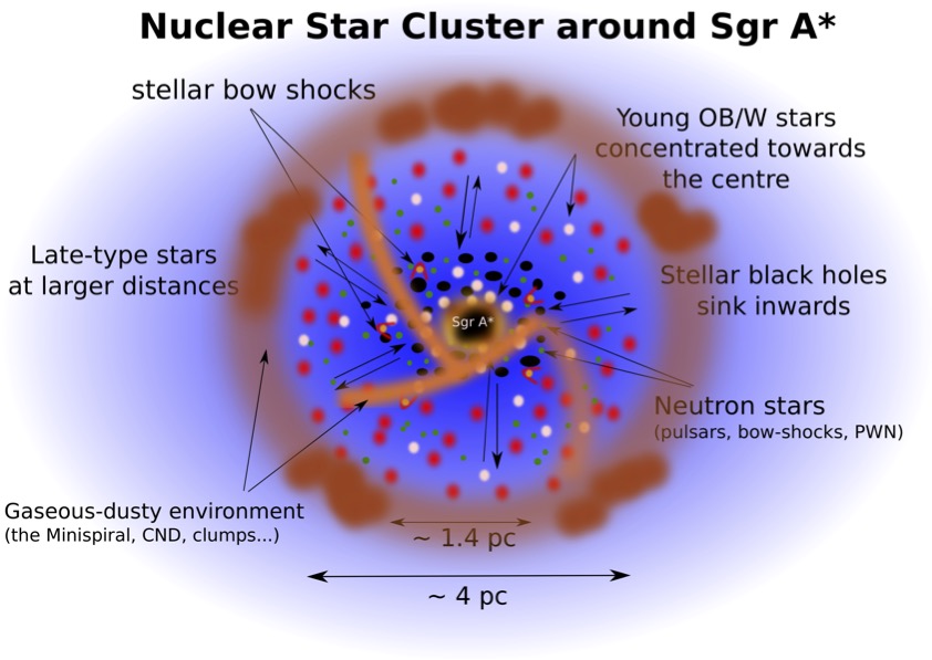
Figure 16: An illustration of the multi-component stellar and gaseous-dusty environment around the compact radio source Sgr A*. The stellar population consists of older, late-type stars whose density appears to decrease towards the centre, at least for bright red giants, forming a distinct flat core. The density of young, massive OB/Wolf-Rayet stars, on the other hand, increases towards Sgr A*, creating a cusp. In the same region, where the Nuclear Star Cluster is located, the interstellar medium is filled with hot, ambient plasma. Denser and partially neutral minispiral arms orbit around Sgr A*, while some of the wind-blowing stars move supersonically through them and form extended bow shocks that are more prominent at longer infrared wavelengths. The population of compact remnants is observationally unexplored in general. Its presence is, however, expected based on the history of massive star-formation in the Galactic centre [458]. The heaviest members – stellar black holes – are expected to sink towards the very centre due to the dynamical friction and kinetic energy equipartition, where they might have formed a steep cusp-like dark cluster.

Although the number density of stars towards the Galactic centre increases as $n_{\star}=n_{0}(r/r_{0})^{-\delta}$ for $\delta>0$, the total number of stars inside the radius $r$, $N_{\star}(<r)$, falls off with the deprojected radius for $0<\delta<3$ since the volume shrinks with $r^{3}$. The observationally determined value of the power-law slope of the stellar density is $\delta<3$, see e.g. Schödel et al., [588] or Genzel et al., [247], with bright late-type stars forming a flat core and early-type stars forming a steeper cusp towards the centre, see Fig. 16 for an illustration. The number of stars can thus fall below one at a certain radius, which marks the volume which lacks stars or one can refer to it as a sparse region, see also Zajaček and Tursunov, [707] for a detailed discussion. As a consequence, it is quite implausible to detect a cluster of stars in the strong-gravity regime, i.e. below 100 Schwarzschild radii. To quantify the length-scale, on which the number of stars is expected to fall below one for a certain stellar type $T$, it is straightforward to calculate the radius $r_{1T}$ at which this is expected to happen. One can obtain the radius $r_{1T}$ from the integral $N_{\star}(<r)=\int_{0}^{r}4\pi r^{2}n_{\star}(r)\mathrm{d}r$ by setting $N_{\star}(<r)=1$ [see also 301, 707],

$$r_{1T}=R_{\rm inf}(C_{\rm T}N_{\rm inf})^{-1/(3-\delta_{\rm T})}\,,$$ (81)

where $R_{\rm inf}$ is the radius of gravitational influence, see Eqs. (43), (79), $N_{\rm inf}$ is the total number of main-sequence stars inside $R_{\rm inf}$, $C_{\rm T}N_{\rm inf}$ is the total number of stars of type $T$ inside $R_{\rm inf}$ and $\delta_{\rm T}$ is the power-law slope of the stellar population of type $T$. Hopman and Alexander, [301] analyzed the inner radius of the stellar cluster for different types of objects, namely main-sequence stars (MSs), white dwarfs (WDs), neutron stars (NSs), and stellar black holes (BHs). They analyzed the properties of the nuclear star cluster and determined that there are in total $N_{\rm inf}\approx 3.4\times 10^{6}$ main-sequence stars inside the influence radius. In Table 1, we list the inner radii of other stellar components of the cluster as calculated by Hopman and Alexander, [301]. According to Table 1, below a few 100 Schwarzschild radii, it is quite unlikely to detect a star that can be used for high-precision tests of general theory of relativity in the highly relativistic regime. This is in particular bad news for the chance of detecting a pulsar around the supermassive black hole in the Galactic center, since it could be used as a precise clock for probing the space-time metric around Sgr A* as first put forward by Paczynski and Trimble, [511]. However, the inner radii listed in Table 1 refer to the stellar cusp in a statistical sense – there could still be a pulsar approaching Sgr A* on the scale of $\sim 10-100$ gravitational radii that was deflected into a highly eccentric orbit due to e.g. dynamical scattering on a massive perturber [531], a binary-star disruption close to the SMBH [706], or a natal velocity kick during the supernova type II explosion in the clockwise stellar disk containing massive OB stars [700, 95].

Table 1: An overview of inner radii of the nuclear stellar cluster for different stellar types $T$ calculated according to Eq. (81) using the dynamical model of Hopman and Alexander, [301].

Population $T$	$C_{\rm T}$	$\delta_{\rm T}$	$r_{1T}\,[\rm pc]$	$r_{1T}\,[r_{\rm S}]$
MS	$1$	$1.4$	$2\times 10^{-4}$	$523$
WD	$10^{-1}$	$1.4$	$7\times 10^{-4}$	$1831$
NS	$10^{-2}$	$1.5$	$2\times 10^{-3}$	$5231$
BH	$10^{-3}$	$2$	$6\times 10^{-4}$	$1569$

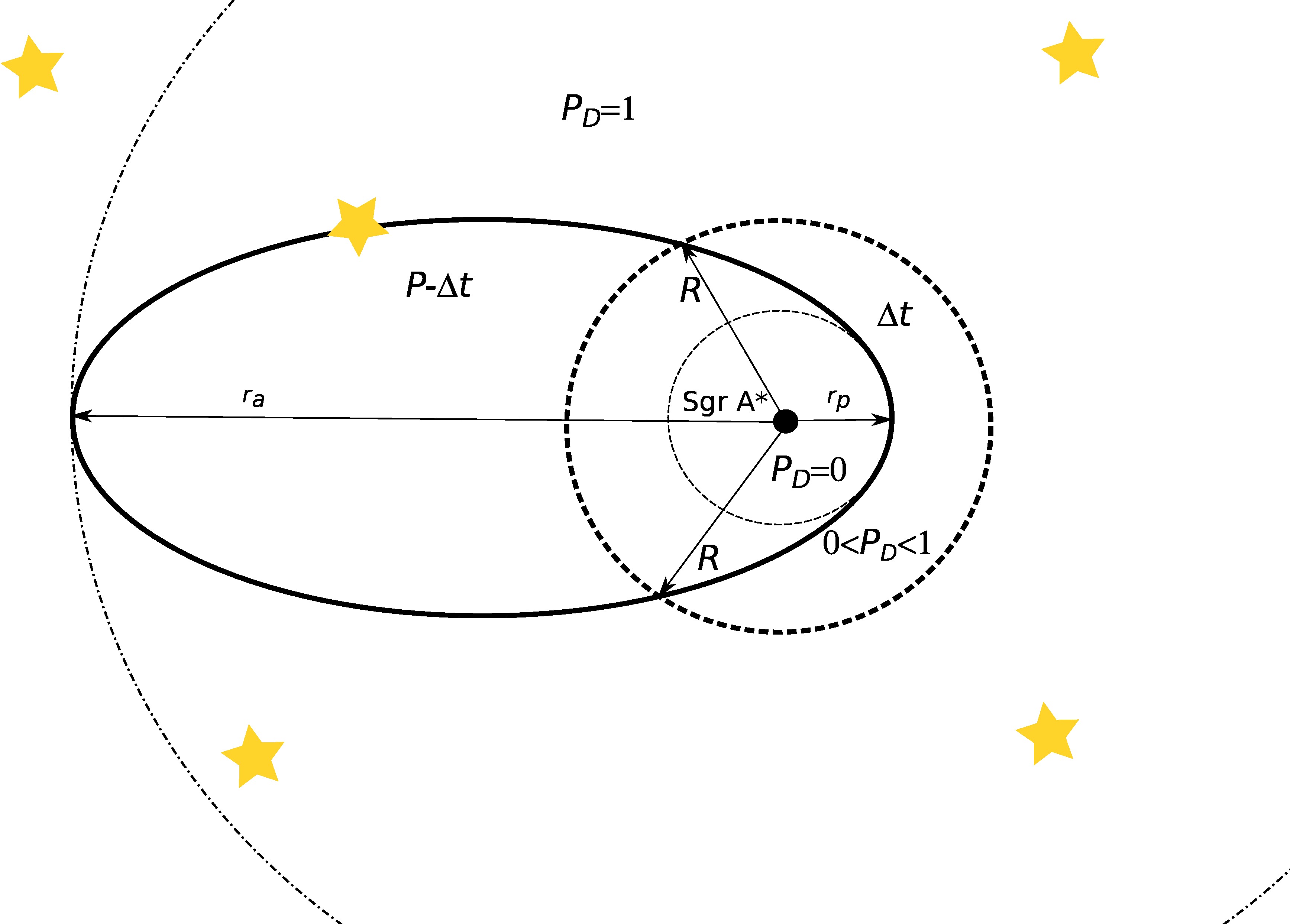
Figure 17: An illustration of the sparse region according to Zajaček and Tursunov, [707]. The star on an eccentric orbit spends the time $\Delta t$ inside a certain region around Sgr A*. The probability of the detection $P_{\rm D}$ can be estimated according to Zajaček and Tursunov, [707]. Adopted from [707].

The set-up of the sparse region is illustrated in Fig. 17. Since inside the S cluster with the radius of 1 arcsecond ($\sim 0.04\,{\rm pc}$) the gravitational potential is dominated by Sgr A*, stellar orbits can be approximated with an ellipse as shown in Fig. 17. Although statistically stars are not expected in this region, they can be scattered into high-eccentric orbits by gravitational encounters with massive perturbers, such as molecular clouds or stellar clusters on the scale of a few parsecs from Sgr A* [531]. The filling of the inner arcsecond by stars via the dynamical scattering on massive perturbers is faster by a factor of $10$–$10^{7}$ in comparison with the classical two-body dynamical relaxation, which takes place on the timescales of a few billion years [434],

$$t_{\rm r} =\frac{0.34\sigma_{\star}^{3}}{G^{2}\rho_{\star}m_{\star}\log{\Lambda}}\,$$

$$=0.95\times 10^{10}\left(\frac{\sigma_{\star}}{200\,{\rm km\,s^{-1}}}\right)^{3}\left(\frac{\rho_{\star}}{10^{6}\,M_{\odot}{\rm pc^{-3}}}\right)^{-1}\left(\frac{m_{\star}}{1\,M_{\odot}}\right)^{-1}\left(\frac{\log{\Lambda}}{15}\right)^{-1}\,{\rm yr}\,$$ (82)

where $\rho_{\star}$ is the stellar mass density, $m_{\star}$ is the mean mass of a single star, and $\log{\Lambda}$ is the Coulomb logarithm, which can be estimated as $\log{\Lambda}\approx\log{(M_{\bullet}/m_{\star})}\sim 15$ for $M_{\bullet}=4\times 10^{6}\,M_{\odot}$ and $m_{\star}=1\,M_{\odot}$.

The non-resonant two-body relaxation normally proceeds slowly and after $\sim 10$ Gyr, the relaxed, steady-state star cluster around a massive black hole is characterized by a cusp-like number density distribution with the slope of $n_{\rm BW}\propto r^{-7/4}$ for equal stellar masses, see Bahcall and Wolf, [33], and $n_{\rm BW}\propto r^{-3/2}$ for unequal stellar masses Bahcall and Wolf, [34]. In the Galactic center, the cusp-like relaxed distribution appears to be the case for faint late-type stars, while bright late-type stars have a flatter core-like distribution [589], which was first recognized based on the drop in the CO bandhead absorption feature inside $\sim 0.5$ pc from Sgr A*, see also Sellgren et al., [593]. This can be attributed to various depletion mechanisms of red giant envelopes that will be described later on.

However, there are faster dynamical processes which can induce plunging, highly-eccentric stellar orbits that refill the “sparse” or “loss-cone” region. First, the non-resonant two-body relaxation timescale expressed by Eq. (82) can be shortened, for the fixed stellar density, by either (i) increasing the perturber mass $m_{\star}$ (molecular clouds, stellar cluster), see the scattering by massive perturbers analyzed by Perets et al., [531], or (ii) decreasing the 1D velocity dispersion $\sigma_{\star}$. The second scenario occurs in stellar disks where the velocity dispersion is small due to nearly corotating orbits in a certain radial bin, see Šubr and Haas, [663]. For instance, in the clockwise disk of young OB/Wolf-Rayet stars having the estimated age of $\sim 6$ Myr [523, 45, 393, 46], the two-body relaxation could have already affected the radial power-law density distribution, and hence the relaxation time is effectively shortened by two-three orders of magnitude in comparison with the spherical cluster of late-type stars.

Once on a tight eccentric orbit, the star gradually descends down the potential well due to gravitational radiation [extreme-mass ratio inspirals – EMRIs; see 19, for a review]. Due to the loss of the orbital energy, the semi-major axis decreases - its time derivative is negative. In addition, the gravitational radiation from the system decreases the eccentricity of an inspiralling star, making the orbit more circular [533]. The characteristic timescale for an EMRI inspiral, given the initial semi-major axis $a_{0}$ and the eccentricity $e_{0}$, is given by the Peters’s relation [533],

$$\tau_{\rm GW}(a_{0},e_{0})\simeq\frac{5}{256}\frac{c^{5}(1+q)^{2}}{G^{3}qM_{\bullet}^{3}}\frac{a_{0}^{4}}{f(e_{0})}\,,$$ (83)

where $q=m_{\star}/M_{\bullet}$ is the mass ratio that we set to $q=2.5\times 10^{-6}$ for $m_{\star}=10\,M_{\odot}$. For the initial distance of $a_{0}=1000\,r_{\rm g}$ and zero eccentricity, we get $\tau_{\rm GW}(1000\,r_{\rm g},0)\simeq 5$ Gyr. The non-zero eccentricity can significantly shorten the inspiral time, e.g. for $e_{0}\sim 0.9$, we obtain $\tau_{\rm GW}(1000\,r_{\rm g},0.9)\sim 4$ Myr, i.e. three orders of magnitude shorter inspiral time. The eccentricity evolution during the gravitational-wave inspiral can be quite complex in realistic scenarios. There are two competing effects as analyzed by Cardoso et al., [117]: (i) due to the gravitational-wave radiation and other vector or scalar backreaction effects, the eccentricity decreases, i.e. the orbit becomes more circular; (ii) the environmental effects, in particular the accretion onto the star or the dynamical friction, lead to the eccentricity increase. The incorporation of these effects is necessary to correctly estimate the EMRI rate for different types of galaxies, in particular the AGN and the quiescent black holes are expected to differ in this regard, and the redshift-dependency of the EMRI rate is also anticipated.

On the scale of a few 10 Schwarzschild radii, the presence of stars and compact objects can be revealed by a quasi-periodic variability due to the regular perturbations of the accretion flow [381, 622]. Quasi-periodic eruptions (QPEs) in the X-ray domain that are present in both AGN as well as quiescent sources [29] are potentially caused by either a matter Roche-lobe overflow from a stellar companion [346, 436] or by the regular passages of a perturber and the associated induced density waves [622]. The inspiral timescale due to the gravitational radiation given by Eq. (83) indicates that two EMRIs can in principle approach each other since for e.g. a twice heavier star the inspiral timescale is shorter by a factor of approximately two. This can lead to gravitationally and even physically interacting pairs of EMRIs of uneven masses, which could be detected via the quasi-periodic pattern in the X-ray light curves, similar to the detected QPEs [435, 436].

Recently, fast-moving stars were also detected with either orbital periods or pericenter distances smaller than the archetypal S2 star. In terms of the orbital period, Meyer et al., [439] identified S0-102/S55 star using W. M. Keck telescope ($K$-band magnitude of $17.1$) with the orbital period of $\sim 11.5$ years, see Fig. 18 for the best-fit orbits, including radial velocities that are colour-coded according to the colour bar on the right. More recently, S62 ($K\sim 16.1$ mag) with the orbital period of $\sim 9.9$ years was identified by Peißker et al., 2020a [526]; see also Gravity Collaboration et al., 2021a [269] and Peißker et al., 2021b [525] for updated analyses. Peißker et al., 2020b [527] discovered so far the shortest-period star S4711 ($K\sim 18.4$ mag) with the orbital period of only $\sim 7.6$ years. In addition to S62 and S4711, several other faint S stars were identified, whose orbital fractions are at least partially inside the S2 orbit. We compare the orbital solutions of these fainter stars, including S62, S4711, and S4712-S4715, with the orbits of S2 and S55/S0-102 in Fig. 18. The most promising candidates for studying relativistic effects are S62 and S4714, which have the smallest pericenter distances of only $\sim 17.8\,{\rm AU}$ ($\sim 450.5$ gravitational radii) and $\sim 12.6\,{\rm AU}$ ($\sim 320.1$ gravitational radii), respectively. This results in the highest potential pericenter orbital velocities of $\sim 20\,000\,{\rm km\,s^{-1}}$ ($\sim 6.7\%$ of the light speed) and $\sim 24\,000\,{\rm km\,s^{-1}}$ ($\sim 8\%$ of the light speed) for S62 and S4714, respectively. These pericenter velocities are at least a factor of two larger than the pericenter velocity of the S2 star, which amounts to $\sim 7600\,{\rm km\,s^{-1}}$ or $\sim 2.5\%$ of the light speed.

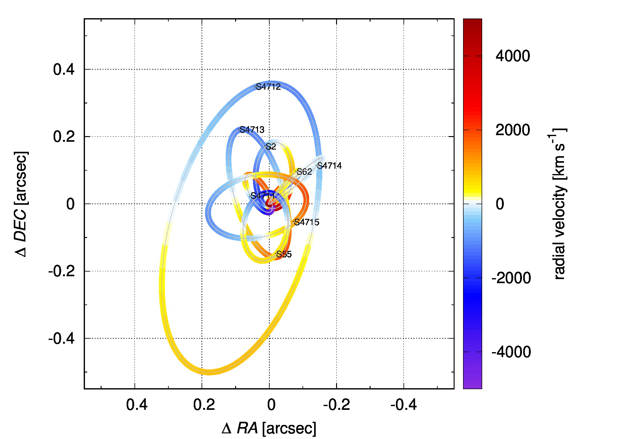
Figure 18: Best-fit orbital solutions of short-period S stars in the Galactic center, including S2 [266], S0-102/S55 [439], and new faint S stars S62 and S4711-S4715 [526, 527]. The sky plane is represented by the right ascension and the declination offsets from Sgr A* in arcseconds. The colour axis on the right represents radial velocities in ${\rm km\,s^{-1}}$. The positions next to text labels depicting individual fast-moving stars correspond to the epoch of $1990.0$.

The lack of stars on the scales of 10 Schwarzschild radii is, however, complemented by orbiting hot spots that orbit Sgr A* close to the innermost stable prograde circular orbit (ISCO) of a nearly Schwarzschild black hole or alternatively, at the retrograde ISCO of a highly-rotating Kerr black hole [267]. These observations were performed by the near-infrared GRAVITY@ESO interferometer, which can resolve out the offset of an emission centroid from Sgr A* with an angular resolution of $\sim 20$–$70\,{\rm\mu as}$. The instrument detected the continuous shift of the centroid position on the length-scales of $150\,{\rm\mu as}$ with the periodicity of $10-30$ minutes. The detected clockwise shift of the emission centroid is consistent with the nearly face-on orbital motion of a denser blob of relativistic electrons that emit non-thermal synchrotron NIR emission. According to the detected positions of the blob, the motion takes place on the scale of $6-10$ gravitational radii $(GM_{\bullet}/c^{2})$. In general, due to uncertainties, the observations suffer from a spin-degeneracy, hence the hot spot orbits Sgr A* close to the prograde ISCO of a nearly Schwarzschild black hole (low-rotating Kerr black hole) or close to the retrograde ISCO of a highly-rotating Kerr black hole. Based on the modulated light curves, flares of Sgr A* modelled by an orbiting hot-spot model can be employed to probe the potential of Sgr A* in a strong-gravity regime, which is currently inaccessible for stars. Light curves of X-ray flares were used to obtain an independent estimate of the mass of Sgr A* [335], which is consistent with the mass determined from stellar astrometry.

The connection between the multi-wavelength variability of Sgr A* and blobs or hot spots orbiting on ISCO scales was already proposed and studied more than a decade before the actual detection of an orbital motion by the GRAVITY experiment [99, 100, 438]. The orbiting hot-spot may result from shocks or magnetic reconnection events in the innermost parts of the hot, magnetized accretion flow [198, 696, 708, 382]. These plasma instabilities can produce a blob of relativistic electrons with the Lorentz factor of $\gamma\sim 10^{3}-10^{6}$, which can explain the multi-wavelength variability of Sgr A* that occurs on hourly timescales. The flares also exhibit the time lags of about one hour between the NIR/X-ray domain and flares at lower frequencies (submillimeter and radio domains), which can be explained by cooling via an adiabatic expansion [198, 696]. In addition, some NIR flares have simultaneous X-ray counterparts which implies the synchrotron-self-Compton (SSC) or inverse Compton process to explain the NIR/X-ray connection [191, 192, 199].

The NIR flares exhibit a correlation between flux modulations and changes in the polarization angle and degree [708]. Zamaninasab et al., [708] showed that the changes in the polarization angle during flares are consistent with the orbital motion of a compact hot spot rather than with the extended emission. This was also confirmed by the GRAVITY experiment [267], which detected a continuous swing of the polarization angle connected with the centroid shift with the same periodicity of $45\pm 15$ minutes as that of the orbital motion. Such a gradual change in the polarization angle may be explained by the hot spot motion in the poloidal magnetic field, i.e. which is perpendicular to the orbital plane.

There are several indications that the magnetic field in the Galactic center is dynamically relevant and ordered on both large and small scales [459, 267]. Concerning the larger scales, the Faraday rotation measurements of the radio emission of the magnetar PSR J1745–2900 [190] put a lower limit on the line-of-sight component of the magnetic field, $B\gtrsim 8\,{\rm mG}$, which is at a deprojected distance of $\gtrsim 0.12\,{\rm pc}$. Eatough et al., [190] also confirmed the ordered structure of the magnetic field at the scale of $0.1\,{\rm pc}$ that is at the intermediate distance between the ordered magnetized filaments in the Central Molecular Zone [459] and the ordered, poloidal magnetic field close to the innermost stable circular orbit of Sgr A* [313, 267]. Since the hot plasma is magnetized and its fraction accretes towards Sgr A*, it is expected to lead to the accumulation of the magnetic flux as the magnetic field lines are dragged inwards by the flow. At a certain distance, at the so-called magnetospheric radius $R_{\rm MAD}$, the accretion flow becomes unstable and fragments since the gravitational potential energy of the flow is comparable to the electromagnetic pressure [471]. Following the energy equipartition, we can approximately derive $R_{\rm MAD}$ based on the equality for the axisymmetric flow [471, 647],

$$\frac{GM_{\bullet}\Sigma}{R_{\rm MAD}^{2}} \approx 2\frac{B_{R}B_{z}}{4\pi}\,\,,$$ (84)

$$R_{\rm MAD} \sim\left(\frac{\sqrt{GM_{\bullet}}\dot{M}}{\sqrt{2}\epsilon B_{\rm pol}^{2}}\right)^{2/5}\,,$$ (85)

$$\sim 68\,\left(\frac{M_{\bullet}}{4\times 10^{6}\,M_{\odot}}\right)^{1/5}\left(\frac{\dot{M}}{10^{-8}\,{\rm M_{\odot}\,yr^{-1}}}\right)^{2/5}\left(\frac{\epsilon}{10^{-2}}\right)^{-2/5}\left(\frac{B_{\rm pol}}{10\,{\rm G}}\right)^{-4/5}\,R_{\rm g}\,,$$ (86)

where $\Sigma=\dot{M}/(2\pi R\epsilon v_{\rm ff})$ is the surface density of the flow, which depends on the accretion rate $\dot{M}$ and the radial velocity $v_{\rm R}=\epsilon v_{\rm ff}$ that is smaller than the free-fall velocity and their ratio is expressed by the parameter $\epsilon\sim 0.01-0.001$ [471]. While deriving Eq. (85), we assumed $B_{R}\sim B_{z}\approx B_{\rm pol}$. Below $R_{\rm MAD}$ the accretion proceeds discretely and diffusely through the poloidal magnetic field, which is refereed to as the magnetically arrested accretion disc [MAD; 76, 77, 471]. For the Galactic center, we estimated $R_{\rm MAD}\sim 68\,R_{\rm g}$ using $\dot{M}\approx 10^{-8}\,M_{\odot}\,{\rm yr^{-1}}$, which is based on the Faraday-rotation measurements [412], and $B_{\rm pol}\sim 10\,{\rm G}$ based on the near-infrared flare observations and modelling their timing and spectral properties [193, 685]. Inside the magnetospheric radius $R_{\rm MAD}$, the accretion flow fragments and proceeds at the radial velocity two to three orders of magnitude smaller than the free-fall velocity [471]. The accretion continues diffusively through the ordered, poloidal magnetic field via magnetic interchanges as well as magnetic reconnection events. The fragmented flow consists of magnetically confined islands. The released energy heats up the surrounding gas, which could observationally be detected as the hot spot orbiting Sgr A* close to the innermost stable circular orbit or just below it, when the heated and outflowing gas spirals in towards the event horizon. This is illustrated in Fig. 19, which connects larger spatial scales, where the hot plasma is fed by stellar winds of $\sim 100$ mass-losing OB/Wolf-Rayet stars, and smaller scales, where the hot flow fragments and proceeds as the clumpy MAD flow below $R_{\rm MAD}$.

The MAD flow – Magnetically Arrested Disk – has a different dynamical set-up than the so-called SANE disk (Standard and Normal Evolution). For the SANE flow, which is only weakly magnetized, the angular momentum is transported outwards via the turbulence generated by the magnetorotational instability [37]. The expected radial division between the SANE and the MAD flow for Sgr A* is given by Eq. (86). Another important length-scale for the Sgr A* accretion flow is the circularization radius $R_{\rm CIR}$, i.e. the distance where the hot flow that possesses an initial angular momentum circularizes. We assume that a circularized thick flow forms with the outer radius of $R_{\rm CIR}$ and that the initial stellar wind material was provided by a star orbiting at $r_{\star}$ with the wind total velocity of $v_{\rm g}$ (including the orbital and the terminal wind velocity). The circularized gas at the outer disk radius has the largest angular momentum, which initially corresponded to the wind material that had at most the escape velocity with respect to Sgr A* at the distance $r_{\star}$, $v_{\rm g}\lesssim(2GM_{\bullet}/r_{\star})^{1/2}$,

$$R_{\rm CIR}\left(\frac{GM_{\bullet}}{R_{\rm CIR}}\right)^{1/2} \approx\lambda r_{\star}v_{\rm g}\lesssim\lambda r_{\star}\left(\frac{2GM_{\bullet}}{r_{\star}}\right)^{1/2}\,$$

$$R_{\rm CIR} \lesssim 2\lambda^{2}r_{\star}\,,$$ (87)

where $\lambda$ is the retained fraction of the initial angular momentum of the stellar wind. The parameter $\lambda$ can be estimated from a few observational indications. Young massive OB/Wolf-Rayet stars with powerful winds are located beyond the S cluster at $r_{\star}\sim 0.1\,{\rm pc}$, i.e. the wind material is captured at the Bondi radius. The circularization radius as such is quite uncertain, however, there is an indication of the colder disk containing ionized $\sim 10^{4}\,{\rm K}$ gas orbiting around Sgr A* as revealed by Murchikova et al., [464] using the hydrogen recombination line H30$\alpha$ at $1.3$ mm. For such a disk with $R_{\rm CIR}\sim 0.004\,{\rm pc}$, the retained fraction of the angular momentum is $\lambda\geq(R_{\rm CIR}/2r_{\star})^{1/2}\sim 0.14$, i.e. at least $\sim 14\%$. In the case of the stellar winds, the angular momentum is expected to be removed by shocks, wind-wind collisions, and the magnetohydrodynamical drag.

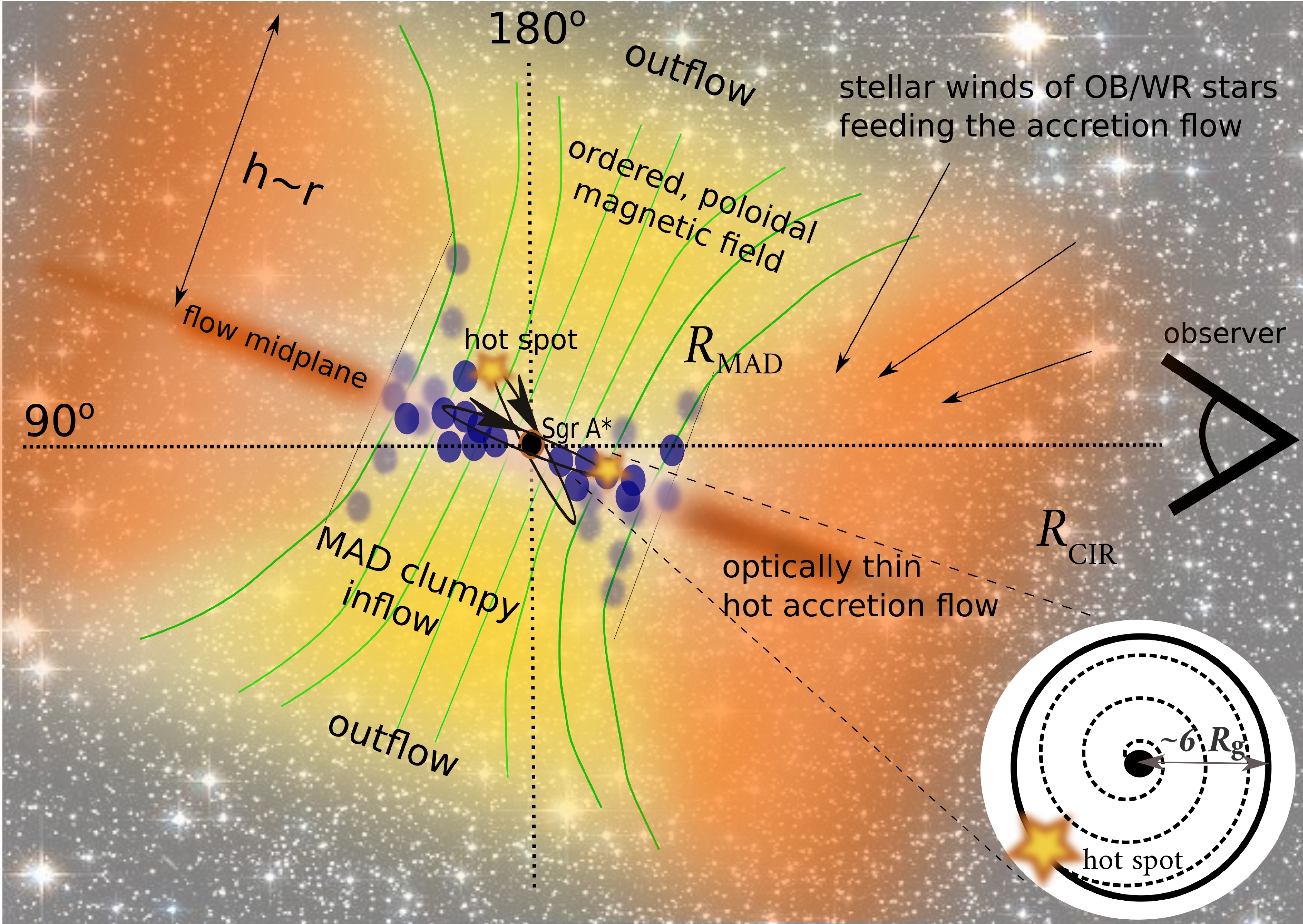
Figure 19: Illustration of the hot accretion flow feeding the variable radio, near-infrared, and X-ray source Sgr A* in the Galactic center. On the larger scales, the cusp of $\sim 100$ mass-losing OB/Wolf-Rayet stars provides the material, a fraction of which is accreted at the Bondi radius [137, 150, 602, 674, 112], $r_{\rm Bondi}\sim 0.14(M_{\bullet}/4\times 10^{6}\,M_{\odot})(T_{\rm g}/1.5\times 10^{7}\,{\rm K})^{-1}\,{\rm pc}$, see Eq. (94). The actual accretion rate of Sgr A* within 100 gravitational radii, $\dot{M}_{\rm acc}\approx 10^{-9}-10^{-7}\,M_{\odot}\,{\rm yr^{-1}}$ [412], is $\lesssim 1\%$ of the Bondi rate, $\dot{M}_{\rm Bondi}\approx 10^{-3}\,M_{\odot}{\rm yr^{-1}}$, which is supplied to a large extent by stellar winds [112]. The poloidal magnetic field frozen in the plasma is dragged inwards, which leads to the accumulation of the magnetic flux in the inner regions. This can result in the development of the magnetically arrested accretion flow [MAD; 76, 77, 471], which is characterized by a slow, diffusive accretion consisting of magnetically confined blobs accompanied by magnetic interchanges and reconnection events. Observationally, the heated expanding gas due to reconnection events could be detected as orbiting “hot spots” that are visible for about one orbital period or its fraction close to the innermost stable circular orbit (ISCO; positioned at 6 gravitational radii for a non-rotating, Schwarzschild black hole), see the figure inset in the right bottom corner. The background image portrays the globular cluster NGC 288 to represent the dense stellar field in the Galactic center; the stellar field of NGC 288 was adopted from the Hubble Space Telescope’s Wide Field Channel of the Advanced Camera for Surveys (credit: ESA/Hubble & NASA).

Localization of Sgr A and Sgr A* – the historical perspective

The first radio source ever observed was the Galactic centre by Karl G. Jansky in 1932 at the frequency of $20.5\,{\rm MHz}$ and the angular resolution of $25^{\circ}\times 35^{\circ}$ while he was working at the Bell Telephone Laboratories. Grote Reber continued in his effort and developed his own radiotelescope and receivers between 1938 and 1948, partially during WWII. He detected the emission from the plane of the Milky Way at the frequency of $160\,{\rm MHz}$ ($1.9$ m), which was peaking towards the Galactic center. Piddington and Minnett, [539] detected a prominent source of radio emission at $1.2\,{\rm GHz}$ and $3\,{\rm GHz}$. The radio emission of the source appeared to be flat between $100\,{\rm MHz}$ and $1210\,{\rm MHz}$, similar to another radio source Taurus A. They proposed that optically thin thermal gas is responsible for the emission and the source became to be known as Sagittarius A (Sgr A). In the mid-1960s Barry Clark and Dave Hogg used the two-element Green Bank interferometer in West Virginia to analyze the small-scale structure of the radio emission with the angular resolution of $10^{\prime\prime}$. They detected a smaller structure inside the Sgr A complex with the flux density of $0.3\,{\rm Jy}$ at $2.8\,{\rm GHz}$ $(11\,{\rm cm})$. However, the source was confused with the thermal emission of Sgr A West [134].

These early observations of the Galactic centre region were essentially simultaneous with the discovery of quasars by Schmidt, [585] in 1963 and the realization that they are extremely distant and luminous thanks to the identification of the redshifted Balmer series of hydrogen in the optical spectra of 3C273. The enormous energy in extragalactic sources – which amounted to $4\times 10^{12}\,L_{\odot}$ for 3C273 in the optical bands – was proposed to originate in large concentrations of mass in their centers and the proposal of ‘giant stars’ powering Seyfert galaxies and quasars, see Hoyle and Fowler, [303]. It was obvious from the first principles that the sudden collapse of mass into relativistic dimensions can yield enough energy to explain the power output of the AGN. Such a mechanism was proposed in the early 1960s by Vitaly L. Ginzburg in the context of the contraction of the central regions of galaxies and the subsequent formation of protostars [258]. Similar and other ideas and theories were presented at the First Texas Symposium on Relativistic Astrophysics in Dallas in December 1963. This event, which is often considered as the “landmark” in the rebirth of relativistic and gravitational astrophysics, brought together theorists and observers of the time. Although the Symposium did not provide final clues to the problem of quasar energetics, it triggered new enthusiasm and pointed astrophysicists in the right direction.

The first original theory of the accretion of gas and dust onto a collapsed object, which releases the thermal and radiative energy due to the conversion of the gravitational potential energy of the infalling matter, was proposed by Yakov Zel’dovich and Igor Novikov [712]. Independently, essentially the same process was described in 1964 by Edwin Salpeter at the Cornell University in the context of massive objects with the mass of $M\gtrsim 10^{6}\,M_{\odot}$ powering quasi-stellar objects [577]. Donald Lynden-Bell generalized the quasar accretion mechanism to other galactic nuclei [395]. Subsequently, Lynden-Bell and Rees, [397] discuss the Galactic centre specifically as a potential location of the “old-quasar” black hole and suggest to use the Very Long Baseline Interferometry (VLBI) to infer its flux density and the position. They also suggested to use objects in the surroundings of the black hole – specifically line-emitting gas – to determine its mass. Soon afterwards, Shakura & Sunyaev presented the solution for an accretion disc where the macroscopic turbulence is responsible for the viscosity [599]. They introduced the $\alpha$ parameter, which relates the viscosity to the sound speed and the disc scale-height, $\nu=\alpha c_{\rm s}H$, and takes values between zero (no accretion) and one. The Shakura & Sunyaev disc is in local thermal equilibrium and radiates away the accumulated viscous heat, cools down, and becomes geometrically thin and optically thick. The general relativistic solution for the thin disc was presented by Novikov and Thorne, [497]. In both works, it is assumed that the viscous torque vanishes at the innermost stable circular orbit (ISCO).

In the same year as the First Texas Symposium, Roy Kerr found the axisymmetric solution to the Einstein field equations [342]. The Kerr solution is applicable to any rotating uncharged mass, including compact objects. Two years later, Ezra Ted Newman generalized the Kerr solution to rotating charged bodies, which is nowadays referred to as Kerr-Newman solution [488], which is the most general asymptotically flat, stationary solution to Einstein-Maxwell field equations. These two solutions followed nearly 50 years after the first static solution of Karl Schwarzschild [591] and the non-rotating charged case of Reissner-Nordström [559, 494]. The overview of all fundamental solutions to Einstein field equations is in Table 2.

Table 2: Overview of fundamental black-hole solutions including the year of their discovery.

Charge/Spin	Non-rotating $(J=0)$	Rotating $(J\neq 0)$
Uncharged $(Q=0)$	Schwarzschild (1916)	Kerr (1963)
Charged $(Q\neq 0)$	Reissner-Nordström (1916,1918)	Kerr-Newman (1965)

Before the identification of the supermassive black hole in the Galactic center, other compact objects were envisaged and discovered, both theoretically and observationally, in parallel with the development of general relativity and quantum mechanics. First, these were the hot and small companions of some visible stars – such as 40 Eridani A, Sirius A, and Procyon. In 1783, William Herschel discovered the two companions of 40 Eridani A – 40 Eridani B and C, where 40 Eridani B was in 1910 spectroscopically identified to be of spectral type A by Williamina Fleming, despite being too faint for spectral type A, which indicated the size of the Earth. Sirius B, which is the nearest white dwarf to the Earth ($\sim 2.64$ pc) was discovered by Alvan Graham Clark on January 31, 1862 in Cambridgeport, Massachusetts. Sirius B as well as other similar faint objects (40 Eridani B, Van Maanen’s star) were later identified as white dwarfs (the name white dwarf was introduced by Willem Jacob Luyten in 1922.), i.e. stellar remnants of low-mass stars supported by degenerate electron pressure with the mean mass density of $\sim 10^{6}\,{\rm g\,cm^{-3}}$. The internal structure of white dwarfs, where are effectively cooling off due to the lack of any thermonuclear fusion, was investigated by Ralph H. Fowler, Edmund Clifton Stoner, Wilhelm Anderson, and Subrahmanyan Chandrasekhar at the end of 1920s and early 1930s using the non-relativistic and relativistic equations of state of degenerate Fermi gas. Solving the hydrostatic equilibrium equation for the relativistic Fermi gas, Chandrasekhar also derived the limit on the mass of stable white dwarfs, which is a function of fundamental constants only,

$$M_{\rm Ch}\approx\frac{\omega_{3}^{0}\sqrt{3\pi}}{2}\left(\frac{\hbar c}{G}\right)^{3/2}\frac{1}{(\mu_{e}m_{\rm H})^{2}}\sim 1.4\,M_{\odot}\,,$$ (88)

where $\omega_{3}^{0}\sim 2$ is the constant related to the solution of the Lane-Emden equation, $\mu_{e}$ is the average molecular weight per electron (here $\mu_{e}=2$), and $m_{\rm H}$ is the hydrogen atom mass. Since $M_{\rm Pl}=\sqrt{\hbar c/G}$ is the definition of the Planck mass, the Chandrasekhar limit can also be roughly estimated using the expression $M_{\rm Ch}\sim M_{\rm Pl}^{3}/m_{\rm H}^{2}\sim 1.9\,M_{\odot}$. Then in 1963, Allan Sandage and Thomas A. Matthews found the first optical counterpart for the bright radio source 3C48 using the 5.1-m Hale telescope atop Mount Palomar, see Matthews and Sandage, [417]. In the same year, also using the Palomar telescope, Maarten Schmidt identified the similar quasi-stellar source 3C273 [585], which is characterized by the radio-optical emission, with a distant extragalactic source with a relatively large redshift of $z=0.158$. As we mentioned, large luminosities of quasars exceeding the host luminosities by two orders of magnitude started to be interpreted by the accretion onto massive compact objects – black holes. However, many experts still considered the concept of black holes purely mathematical. When the first pulsar (PSR B1919$+$21) with the periodicity of only 1.33730 seconds was discovered on August 6, 1967 by Jocelyn Bell [288], it was clear that even more compact objects than white dwarfs do exist. The concept of fast-spinning neutron stars having the mean densities of $\sim 10^{14}\,{\rm g\,cm^{-3}}$ and with the radius of only $\sim 10$ km was already theoretically laid out by Baade and Zwicky, [31] and Landau, [373]. Neutron stars provided a natural explanation for periods of the order of one second since any larger object than $R_{\rm limit}\sim[GM_{\rm Ch}P_{\rm rot}^{2}/(4\pi^{2})]^{1/3}\sim 1700\,{\rm km}$ would be unstable and break up at the rotational periods of $P_{\rm rot}\sim 1\,{\rm s}$. Later discovered millisecond pulsars, the first of which with the period of $1.558\,{\rm ms}$ (PSR B1937$+$21) was discovered by Backer et al., [32], constrained the radius to less than $\sim 170\,{\rm km}$. Hence, the concept of the continuing collapse, or rather of the inevitable formation of space-time singularities beyond certain threshold, later called the event horizon, see Penrose, [530], and hence the concept of black holes became rather realistic after the consecutive discoveries of white dwarfs, the first quasars, and pulsars. The mass limit for the formation of neutron stars during the stellar collapse is given by the Chandrasekhar limit, see Eq. (88), i.e. stellar end-products heavier than the Chandrasekhar mass will end up as neutron stars supported by the pressure of degenerate neutrons. The mass limit separating neutron stars from black holes is less clear but it has followed from the work of Richard C. Tolman, who developed the method for solving nonlinear Einstein’s field equations for static spheres filled with fluid [642]. Shortly before the WWII, in 1939, J. Robert Oppenheimer and George Volkoff derived the equation describing the static state of spherically symmetric spacetimes filled with fluid with pressure $P(r)$, now known as the Tolman-Oppenheimer-Volkoff (TOV) equation, which is essentially the general relativistic equation of hydrostatic equilibrium,

$$\frac{\mathrm{d}P}{\mathrm{d}r}=-\frac{G}{r^{2}}\left[\rho+\frac{P(r)}{c^{2}}\right]\left[m(r)+\frac{4\pi r^{3}P(r)}{c^{2}}\right]\left[1-\frac{2Gm(r)}{c^{2}}\right]^{-1}\,,$$ (89)

where $m(r)$ is an enclosed mass within the distance $r$, $P(r)$ is the pressure, and $\rho(r)$ is density. When relativistic corrections are too small, the terms with $1/c^{2}$ can be neglected, which leads to the Newtonian equation of hydrostatic equilibrium describing static, spherically symmetric structure of matter, $\mathrm{d}P/\mathrm{d}r=-Gm(r)\rho(r)/r^{2}$. In the paper from 1939 titled “On Massive Neutron Cores" [500], J. Robert Oppenheimer and George Volkoff derived the maximum mass of a neutron star, using the TOV equation and an equation of state of a degenerate Fermi gas of neutrons. They arrived at the value of $0.7\,M_{\odot}$, too low given the current values for the maximum or the TOV mass limit, which is in the range of $M_{\rm TOV}\approx 1.5-3\,M_{\odot}$ [601, 91]. Kalogera and Baym, [315] found a slightly smaller range towards larger masses, $M_{\rm TOV}\approx 2.2-2.9\,M_{\odot}$. This discrepancy can be explained by the usage of an inadequate equation of state by Oppenheimer and Volkoff, which neglected the short-range nuclear repulsive force among neutrons. The value of the TOV limit was recently constrained based on the gravitational-wave detections of neutron star-neutron star mergers as well as based on the follow-up electromagnetic detections, mainly associated with the first such detection GW170817 [1]. The analysis of GW170817 data constrained the TOV limit to $M_{\rm TOV}\lesssim 2.3\,M_{\odot}$ [604] for cold spherical neutron stars. Hence, the existence of the Chandrasekhar and TOV limits implies the three stable end-states of the stellar matter – white dwarfs, neutron stars, and black holes. Black holes as such occupy the largest mass range from $M_{\rm TOV}$ up to essentially $\sim 10^{10}\,M_{\odot}$. In general, the division into stellar, intermediate-mass, and supermassive black holes is often introduced depending on the mass. These three classes of black holes likely have the common origin in stars or cosmologically in collapsing gas clouds and the further increment in mass depends on the dynamical and magnetohydrodynamic state of the surrounding medium where the black hole is located.

Finally, a compact radio source later denoted as Sgr A* was discovered by Bruce Balick and Robert Brown on February 13 and 15, 1974, which showed a brightness temperature in excess of $\sim 10^{7}\,{\rm K}$ and was unresolved at $<0.1^{\prime\prime}$. To resolve such a compact object among the extended radio emission of the angular size of $\lesssim 20^{\prime\prime}$ was made possible thanks to the newly commissioned interferometer Green Bank – Huntersville (National Radio Astronomy Observatory – NRAO) with the longest baseline of $35$ km. It consisted of three $26$-meter telescopes in Green Bank, which were separated by $\lesssim 2.7\,{\rm km}$ and the newly-installed $14$-meter radio telescope on the mountaintop in Huntersville separated by $35\,{\rm km}$ from Green Bank. The Green Bank–Huntersville interferometer could observe at $11\,{\rm cm}$ and $3.7\,{\rm cm}$ simultaneously.

The compactness of the source, its high brightness temperature, and the association of the radio source with the Galactic center made Sgr A* a suitable candidate for the Milky Way supermassive black hole as hypothesized by Lynden-Bell and Rees [397]. The basic properties were confirmed by higher-resolution Very Long Baseline Interferometry (VLBI) radio observations at $3.7$ cm by Lo et al., [390], who resolved out Sgr A* down to $\lesssim 0.02^{\prime\prime}$ using the $242\,{\rm km}$ baseline. The measured flux density of $F_{3.7}=0.6\pm 0.1\,{\rm Jy}$ implied the brightness temperature of

$$T_{\rm B} =\frac{F_{\nu}c^{2}}{2\nu^{2}k_{\rm B}\pi\theta^{2}}\,$$

$$\sim 10^{7}\left(\frac{F_{\nu}}{0.6\,{\rm Jy}}\right)\left(\frac{\nu}{8\,{\rm GHz}}\right)^{-2}\left(\frac{\theta}{0.02^{\prime\prime}}\right)^{-2}\,{\rm K}\,,$$ (90)

that is based on the Rayleigh-Jeans approximation, $h\nu\ll k_{\rm B}T_{\rm B}$, which is certainly valid in the radio domain ($h\nu\sim 5.4\times 10^{-17}\,{\rm erg}$ while $k_{\rm B}T_{\rm B}\sim 1.38\times 10^{-9}\,{\rm erg}$, i.e. thermal energy per particle is 8 orders of magnitude larger). In addition, based on the comparison with the previous radio data, they inferred that the source is variable.

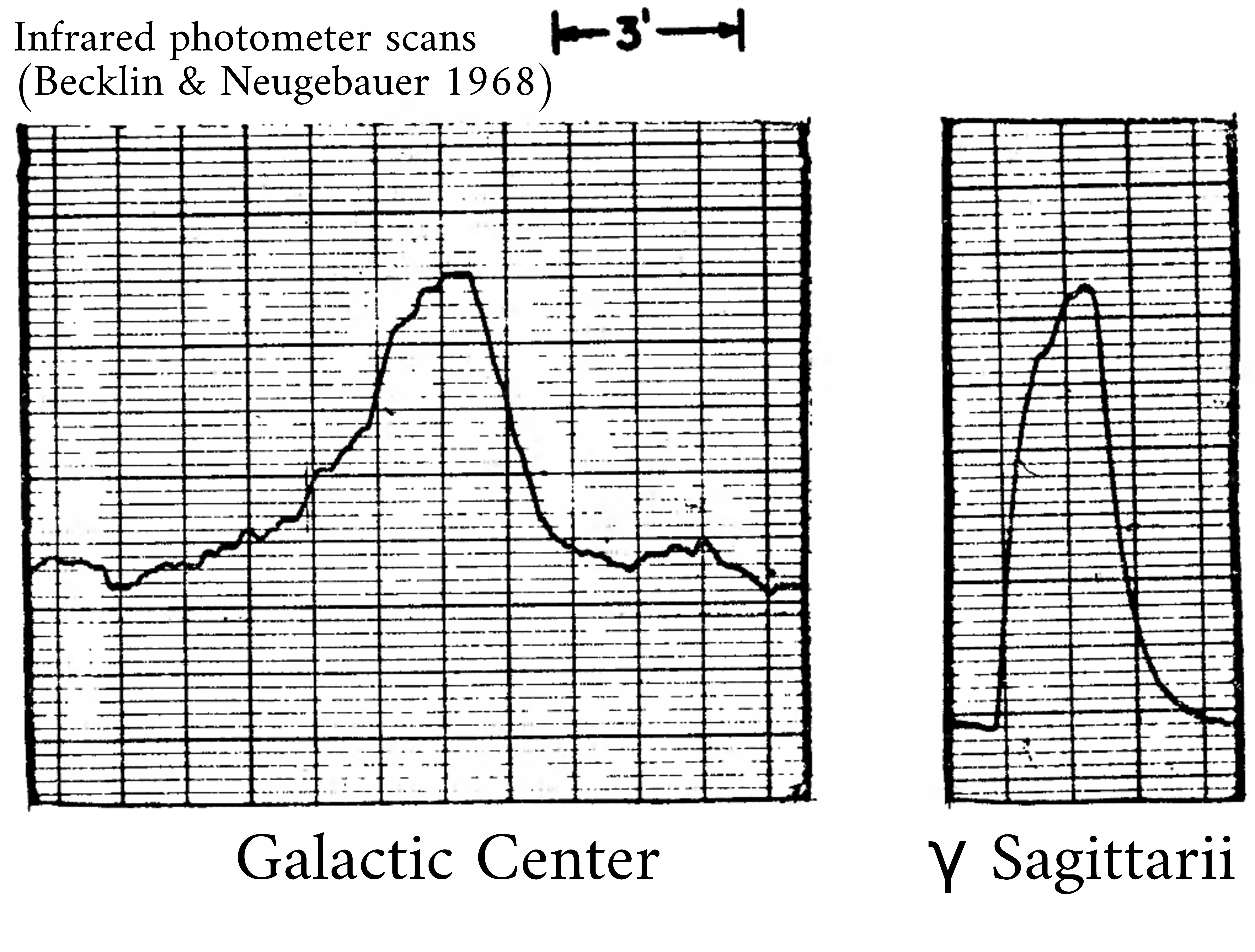
Figure 20: The infrared photometer scan along the right ascension at the wavelength of $2.2\,{\rm\mu m}$. To the left, the Galactic center brightness profile is shown, while to the right, the star $\gamma$ Sagitarii is shown for comparison. The strip-chart image was taken from Becklin and Neugebauer, [51].

In parallel to the first radio observations of the Galactic center, there had also been the first attempts to detect Sgr A* and its surroundings in the infrared domain. Infrared light can penetrate through the dust along the line of sight much better than the optical or the UV radiation that is either absorbed or scattered. The first attempts to detect the Galactic center in the infrared domain were performed in 1945, but due to a lack of sensitivity as well as a coarse sampling , these observations conducted at 1 micrometer were not successful in detecting the Galactic center complex without confusion [615]; see also Moroz, [457]. However, Stebbins and Whitford, [615] found an indication for the infrared source behind the dust clouds and suggest to perform observations at $2\,{\rm\mu m}$. This was followed up by Eric Becklin and Gerry Neugebauer [51], who used the military infrared photometer with the PbS detector mounted at the Mount Wilson and the Palomar observatories with the angular resolution between $1.8^{\prime}$ and $0.08^{\prime}$ that corresponds to the linear scales of $4.2$ and $0.2$ parsecs, respectively, at the distance of the Galactic center. They managed to resolve out the nuclear star cluster that was characterized by a sharp symmetric peak in the $2.2\,{\rm\mu m}$ flux density along the Galactic plane, see Fig. 20. In addition, they also resolved out individual stellar complexes within the cluster using individual bolometer scans. They interpret the central emission seen in the right-ascension scan as a stellar emission of the central cluster with the effective photosphere temperature exceeding $\sim 4000\,{\rm K}$. However, a non-thermal contribution to the thermal stellar emission cannot be excluded, especially in the central part.

The infrared observations using the fine-structure NeII line at $12.8\,{\rm\mu m}$ detected in emission revealed the supersonic and ordered motion of the ionized gas, with the centroid of the NeII line of $+75\pm 20\,{\rm km\,s^{-1}}$ and the velocity dispersion of $200\,{\rm km\,s^{-1}}$ [686]. In particular, Wollman et al., [687] detected the preferentially redshifted neon-emitting gas in the eastern part of Sgr A West that could have been separated from the blueshifted gas in the western part. Based on the Doppler velocities in the range from $+250\,{\rm km\,s^{-1}}$ to $-350\,{\rm km\,s^{-1}}$, the total enclosed mass within $1\,{\rm pc}$ was estimated to $\sim 4\times 10^{6}\,M_{\odot}$. A more detailed spatial distribution as well as the dynamics of Sgr A West inferred from the NeII line were presented by Lacy et al., [370] and Lacy et al., [371]. They revealed that the gas is kept ionized by stars with $T_{\rm eff}\lesssim 35\,000\,{\rm K}$ and that Sgr A West or minispiral clouds are transient in nature with the lifetime of $1\,000-10\,000$ years. With the inauguration of the Very Large Array in 1980, it was possible to produce the 5 GHz radio map of Sgr A West with the comparable angular resolution of $2^{\prime\prime}\times 8^{\prime\prime}$ as that of the infrared images at $10\,{\rm\mu m}$ [105]. Both the radio and the infrared images exhibited the similar structures, in particular the infrared thermal emission peaks corresponded to the peaks in the radio continuum. The ratio of the flux densities of the discrete sources between the infrared and the radio domains was high, $\sim 100-1000$, which indicated the ionization by the soft thermal spectral energy distribution corresponding to $\sim 25\,000\,{\rm K}$, i.e. by the OB stars in the central stellar cluster.

The designation Sgr A* was adopted for the first time by Robert Brown [104] to distinguish the variable non-thermal compact source from the more extended thermal region Sgr A West.

Sgr A* and the environment of its SMBH

The detection of stellar proper motions, the measurement of radial velocities and mainly the fitted quasi-Keplerian orbits of stars in the innermost arcsecond from the compact radio source Sgr A* led to the very reliable determination of the mass of the central dark object, $M_{\bullet}\simeq 4\times 10^{6}\,{M_{\odot}}$ [194, 195, 252, 590, 256, 88, 522, 257].

Under the assumption that Sgr A* is a black hole, the corresponding Schwarzschild radius is $R_{\rm Schw}=1.2\times 10^{12}\,{\rm cm}(M_{\bullet}/4\times 10^{6}\,M_{\odot})$ and the expected mean density is,

$$\rho_{\bullet}=1.7\times 10^{25}\left(\frac{M_{\bullet}}{4\times 10^{6}\,M_{\odot}}\right)\left(\frac{R_{\rm Schw}}{3.9\times 10^{-7}\,{\rm pc}}\right)^{-3}\,M_{\odot}{\rm pc^{-3}}\,.$$ (91)

If the measurements of the orbiting matter (stars and hot gas) approach this value, we can consider Sgr A* to be a black hole in a classical relativistic sense for simplicity, excluding extended configurations such as a cluster of old compact remnants. On the other hand, it is experimentally very difficult to distinguish a black hole from other very compact configurations of matter that lack an event horizon, such as boson stars, fermion balls, and other options [for a general discussion and the notion of “macroquantumness”, read more in 197].

Among the determined stellar orbits in the innermost stellar cluster [so-called S cluster; see the pioneering works by 194, 195, 252], the tightest constraint for the density of the dark mass comes from the monitoring of B-type star S2 (or S0-2) with the pericentre distance of $r_{\rm P}\simeq 5.8\times 10^{-4}\,{\rm pc}$ [522, 590, 256, 257]

$$\rho_{\rm S2}=5.2\times 10^{15}\left(\frac{M_{\bullet}}{4.3\times 10^{6}\,M_{\odot}}\right)\left(\frac{r_{\rm P}}{5.8\times 10^{-4}\,{\rm pc}}\right)^{-3}\,M_{\odot}{\rm pc^{-3}}\,.$$ (92)

The largest density constraint is given by 3$\sigma$ Very Long Baseline Interferometry (VLBI)measured source size of $\sim 37\mu{\rm as}$ [178], which in combination with the lower mass limit of $M_{\rm SgrA*}\gtrsim 4\times 10^{5}\,M_{\odot}$ based on the proper motion measurements [558], yields the density lower limit of $\rho_{\rm SgrA*}\geq 9.3\times 10^{22}\,M_{\odot}\;{\rm pc^{-3}}$. This is only about two orders of magnitude less than the density expected for a black hole of $\sim 4\times 10^{6}\,M_{\odot}$, see Eq. (91). When taking into account the overall stability of this dark concentration of mass over the Galaxy lifetime of $\sim 10^{10}\,{\rm yr}$, the most plausible stable configuration that can explain such a large concentration of mass within a small volume emerges within the framework of general relativity: a singularity surrounded by an event horizon – a black hole, ruling out most of the unstable alternatives [197], such as dense stellar clusters and boson stars.

From multi-wavelength observations over the past fifty years, ranging from radio, millimeter, sub-millimeter, through infrared, X-ray, up to gamma-ray wavelengths, see Genzel et al., [247] for a review, it has become clear that the supermassive black hole associated with the compact radio source Sgr A* is not surrounded by vacuum. Instead, it is embedded in the Nuclear Star Cluster (NSC), which is one of the densest stellar clusters in the Galaxy [587], as well as in the multi-phase gas and dust environment [461].

In Fig. 16, we illustrate different components of the inner portions of the Galaxy. The figure captures the clumpy Circum-Nuclear Disk (CND), which is mostly composed of warm $(\sim 100\,{\rm K})$ neutral and molecular gas of the total mass of $M_{\rm CND}\approx 10^{5}\,M_{\odot}$ and the number densities of $n_{\rm CND}\approx 10^{4}-10^{7}\,{\rm cm^{-3}}$ [249, 596, 276, 443, 131, 561, 447]. The peak of the molecular emission is at $\sim 1.6\,{\rm pc}$ from Sgr A*. However, the outer edge of the CND at $\sim 4-7\,{\rm pc}$ approximately coincides with the outer edge of the Nuclear Star Cluster. The inner edge of the CND is rather sharp at $\sim 1.5\,{\rm pc}$, where the gas density drops below $\sim 10^{4}\,{\rm cm^{-3}}$ [86]. This inner part is also denoted as the central cavity, which is composed mostly of rarefied gas ionized by hot massive OB stars in this region, see Blank et al., [86] and references therein. The central cavity is considered to be refilled with the gas from the CND due to the interaction between its inner rim and an almost spherical outflow from the central stellar cluster, see Fig. 21 for an illustration.

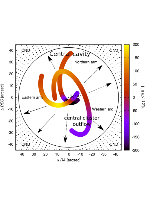
Figure 21: Projected positions of the Circum-Nuclear Disk (CND) and the Minispiral arms. The Minispiral is color-coded to express radial-velocities of the emitting ionized gas along the three arms according to the quasi-Keplerian model of Zhao et al., [716]. The inner rim of the clumpy CND is located at $\sim 1.5\,{\rm pc}$, where the region of rarefied ionized gas – the so-called Central Cavity – is located. The central outflow from the central stellar cluster centered at Sgr A* plausibly interacts with the inner rim of the CND, whose material fills the cavity. This region is, however, not quite homogeneous and spherically symmetric. Several gaseous phases – ionized, neutral, molecular – as well as dust grains are located in the central region.

However, the medium in the central cavity is in general multi-phase, with the three Minispiral arms (also denoted as thermal Sgr A West) reaching larger gas densities of a few of $\sim 10^{4}\,{\rm cm^{-3}}$ [717, 716] in comparison with the hot plasma in their surroundings. The gas in the arms is mostly ionized and has the electron temperature of $\sim 5\,000-13\,000\,{\rm K}$ [716, 369]. The Minispiral arms have a total gas mass of $\sim 100\,M_{\odot}$ and the Northern and the Western arms are considered to be ionized inner parts of the CND [131]. The dynamics of the three arms can be fitted by three bundles of quasi-Keplerian ellipses with Sgr A* at the focus [716]. Molecular gas is detected in Sgr A West as well [461], mostly outside of the Minispiral arms that are predominantly ionized. In Fig. 22, three different phases are depicted: ionized gas (blue; based on 250 GHz continuum observations with ALMA, $0.75^{\prime\prime}$ beam), molecular gas (green; CS$(5-4)$ line-emission observations with ALMA, $0.75^{\prime\prime}$ beam), stars and warm dust (red; $3.8\,{\rm\mu m}$ observations with VLT).

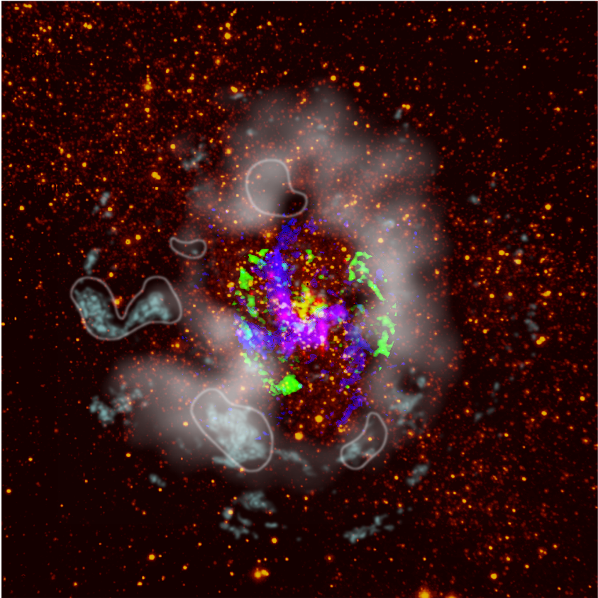
Figure 22: Combined near-infrared, sub-mm, and inverted X-ray image of the innermost 5.6 $\times$ 5.6 parsecs of the Galactic centre. Colors represent different structures and phases of matter: ionized gas (blue; based on 250 GHz continuum and H39$\alpha$ recombination line observations with ALMA, $0.75^{\prime\prime}$ beam; Moser et al., , 2017), molecular gas at the inner rim of the circumnuclear disk (green; CS$(5-4)$ line-emission observations with ALMA, $0.75^{\prime\prime}$ beam; Moser et al., , 2017), stars and warm dust (red; $3.8\,{\rm\mu m}$ L’-band observations with VLT NACO; Sabha et al., , 2012). On the larger scales, the extended white ring marks the footprint of the circumnuclear disk that is seen as a depression in the X-ray diffuse emission, see Mossoux and Eckart, [462] for the detection and the detailed analysis. The stellar background consists of yellow point sources and it is the combination of ISAAC 1.19, 1.71, and 2.25 ${\rm\mu m}$ narrow-band images, see Nishiyama and Schödel, [490] for details. The cyan patches along the circumnuclear disk stand for $N_{2}H^{+}\,(1-0)$ molecular complexes [461], the largest of which coincide with the dark extinction regions in the near-infrared domain (encircled regions). These are dense molecular clouds that are candidates for star-forming regions in the central $\sim 10\,{\rm pc}$ from Sgr A*. Figure adopted from Eckart et al., [200], courtesy of Moser et al., [461], Mossoux and Eckart, [462].

Because of the presence of other bodies in the vicinity of Sgr A*, the classical general-relativistic solutions derived for vacuum, i.e. Kerr-Newman metric in the most general form (which turns into the Kerr metric for the assumed zero electric charge and subsequently the Schwarzschild case for an uncharged non-rotating black hole), are basically not valid. However, since typical stars and gas clouds have negligible masses in comparison with Sgr A*, they can be treated as test particles in most relevant cases. In many cases, it is sufficient to treat the motion of stars in the post-Newtonian framework [573]. When necessary, the motion of test particles can be calculated for the Kerr metric with relevant perturbation effects of the stellar cluster and the gaseous-dusty structures. In particular, general-relativistic treatment of self-gravitating disks and rings made up of stars and gas was analyzed [323, 594, 595, 684]. Such structures can be detected in the standard AGN model (standard thin Shakura-Sunyaev accretion disk) as well as in the Nuclear Star Cluster around Sgr A* in the form of the Clock-Wise stellar disk [46] between $0.05$ and $0.5$ parsecs. The analysis of the 3D dynamical state of the S cluster revealed that it consists of at least two nearly perpendicular stellar disks, i.e. the stellar distribution deviates significantly from isotropy [17].

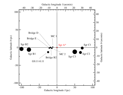
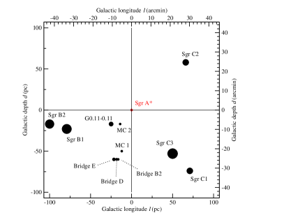
Figure 23: Positions of the molecular clouds around Sgr A* [456, 116] can be reconstructed with improved precision of future X-ray imaging polarimetry, assuming that the primary radiation signal from the SMBH accretion has been scattered towards the observer [409]. Left panel is oriented along the edge-on view (as seen from Earth), whereas the right panel shows the perpendicular view, i.e. from the perspective of the pole-on direction.

Koyama et al., [359] suggested that the X-ray emission, and in particular the intensity of 6.7 keV iron line speak in favour of presence of interstellar medium shock-heated by an energetic explosion. Although Sgr A* appears to be very quiet and underluminous in its present state, there is circumstantial evidence for much more vigorous activity in the relatively recent history over past few hundred years. The evidence has been accumulated for at least two high-luminosity phases during which the SMBH environment was illuminated by intense X-rays [625, 306, 545]. Going back in the history, the activity can be recognized in the early broadband (15 arcmin resolution) images from Granat satellite [626]. Indeed, in order to probe the enormously crowded field surrounding Sgr A*, an excellent imaging capability is essential. But in addition to it, the imaging polarimetry can constrain the physical processes with much higher confidence. Especially the scenario of centrally illuminated distribution of clouds orbiting the SMBH automatically suggests a possibility of a polarized signal (the reflection component) and the polarization angle and degree can be used to trace the 3D positions of the clouds [408].

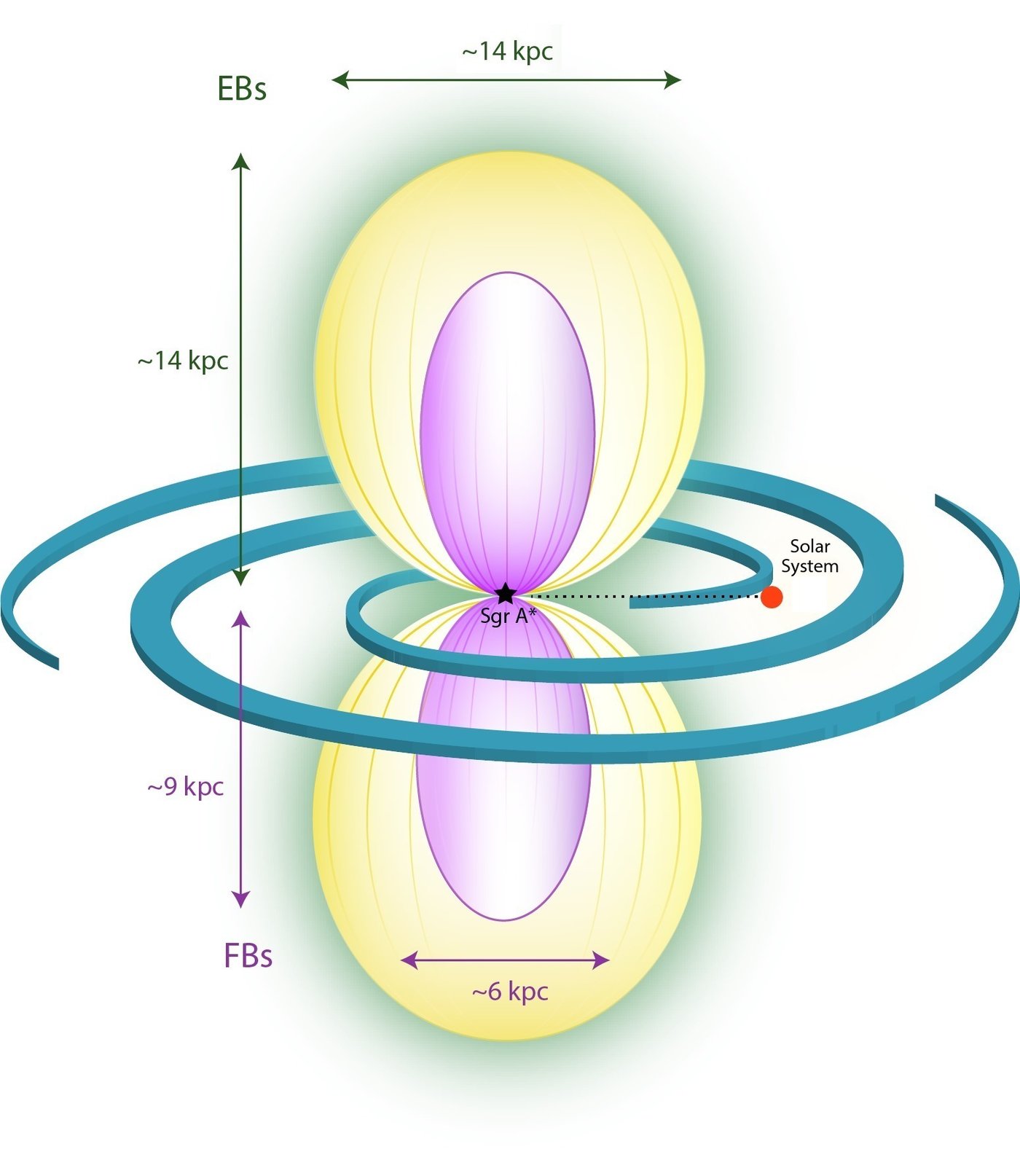
Figure 24: A schematic comparison of the size of the X-ray eROSITA bubbles (EBs) surrounding the previously discovered $\gamma$-ray Fermi bubbles (FBs) above and below the Galactic plane. The inflated bubbles seen in the X-ray domain have the length-scale comparable with the whole Galactic disk and they are clearly larger than the more compact $\gamma$-ray Fermi bubbles. For a detailed description of the observational analysis of eROSITA data; see Predehl et al., [546]. Image credit: Max Planck Institute for Extraterrestrial physics.

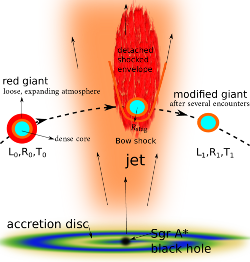
Figure 25: A scheme of the jet-ablation mechanism that likely operated in the Galactic center during the previous Seyfer-like state. As the red giant with a loose, expanding atmosphere enters the jet, its envelope is shocked and partially detached. After the interaction, the giant is truncated and has a higher effective temperature and a smaller infrared luminosity. For details, see Zajaček et al., 2020a [698]. Adopted from Zajaček et al., 2020b [699].

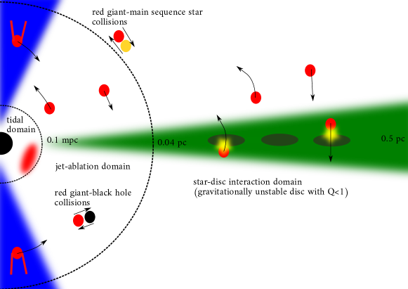
Figure 26: Illustration of different mechanisms that likely contributed to the observed dearth of bright red giants in the Galactic center. At smaller scales, the tidal disruption dominated, while further away the loose red-giant envelopes were ablated and removed via the collisions with the denser parts of the accretion disk. At intermediate scales, the jet-ablation likely contributed to the depletion of the brightest red giants. Adopted from Zajaček et al., 2020b [699].

Every few million years the Galactic center is expected to significantly increase its activity by several orders of magnitude in terms of the bolometric accretion luminosity. During this Seyfert-like stage, Sgr A* was surrounded by a dense accretion disk that could also have powered a bipolar jet with the kinetic luminosity of $10^{41}-10^{44}\,{\rm erg\,s^{-1}}$ for $\sim 0.1-1.0$ Myr, see Zajaček et al., 2020a [698] and references therein. One of the traces of such an enhanced activity could be large-scale $\gamma$-ray Fermi bubbles [621] and even more extended eRosita bubbles [546] that could have been inflated by the nuclear outflow or a collimated jet. The alternative theory of their inflation is the recent nuclear starburst accompanied by supernova explosions, but this seems to be currently ruled out based on energetic grounds [80]. The X-ray eRosita bubbles with the length-scale of $\sim 14\,{\rm kpc}$ are larger than the $\gamma$-ray Fermi bubbles ($\sim 9\,{\rm kpc}$), see Fig. 24 for the comparison of both large-scale structures. Another signature of the enhanced accretion and jet activity of Sgr A* in the past million years could be missing bright red giants. Evolved late-type stars can form CO molecules in their atmospheres and inside $\sim 0.5\,{\rm pc}$, these is a drop in the CO bandhead absorption, which indicates that there is a decrease in the number of red giants close to Sgr A* [593]. More precisely, bright red giants exhibit a flat stellar surface-density distribution while fainter late-type stars have a cuspy surface-density profile [589], which indicates that a preferential depletion of larger, brighter red giants took place. The jet activity fits into this scenario of the preferential destruction of bright red giants since it can effectively ablate the upper layers of diluted and extended red-giant envelopes [510], which would lead to its decreased infrared luminosity [698], see Fig. 25 for the illustration. The jet-ablation can complement other mechanisms of the red-giant depletion in the Galactic center: on smaller scales, the tidal disruption of red giants operates, while further away the red giants suffer ablation and mass loss while passing through the denser parts of the accretion disk. In addition, star-star and star-compact remnant collisions can contribute to the red-giant destruction, see Fig. 26 for the illustration of different mechanisms.

Sgr A* and hot accretion flows

The compact radio source Sgr A* is a very faint source in comparison with active galactic nuclei, with the bolometric (accretion) luminosity several orders of magnitude below its Eddington limit. With the measured bolometric luminosity of $L_{\rm Sgr~{}A*}\lesssim 10^{37}\,{\rm erg\,s^{-1}}$ [472, 247, 197] and the mass of $M_{\bullet}\simeq 4\times 10^{6}\,M_{\odot}$, the Eddington ratio for Sgr A* is,

$$\lambda_{\rm Edd}=\frac{L_{\rm SgrA*}}{L_{\rm Edd}}\lesssim\frac{10^{37}\,{\rm erg\,s^{-1}}}{5.2\times 10^{44}\,{\rm erg\,s^{-1}}}\approx 1.9\times 10^{-8}\,,$$ (93)

i.e., Sgr A* is eight to nine orders of magnitude below the Eddington limit for $4\times 10^{6}\,M_{\odot}$ black hole. From the Faraday rotation measurements of Sgr A*, Marrone et al., [412] inferred the upper and the lower limit of the accretion rate, $\dot{M}_{\rm acc}=2\times 10^{-7}\,{\rm M_{\odot}\,yr^{-1}}$ and $\dot{M}_{\rm acc}=2\times 10^{-9}\,{\rm M_{\odot}\,yr^{-1}}$, respectively. The source of the material are potentially the stellar winds of $\sim 100$ massive Wolf-Rayet (WR) of spectral types O and B that orbit the black hole in the innermost one parsec [393, 46]. The gas from stellar winds is captured by the gravitational pull of the black hole within the Bondi radius $r_{\rm B}$ [93], at which the gravitational potential of Sgr A* overcomes the thermal pressure of the ionized plasma,

$$r_{\rm B}\simeq\frac{2GM_{\bullet}}{c_{\rm s}^{2}}\approx 0.15\left(\frac{M_{\bullet}}{4\times 10^{6}\,M_{\odot}}\right)\left(\frac{\mu_{\rm HII}}{0.5}\right)\left(\frac{\gamma}{1.4}\right)^{-1}\left(\frac{T_{\rm p}}{10^{7}\,{\rm K}}\right)^{-1}\,{\rm pc}\,,$$ (94)

where the mean atomic weight is set to $\mu_{\rm HII}=0.5$, which corresponds to the fully ionized plasma or HII region.

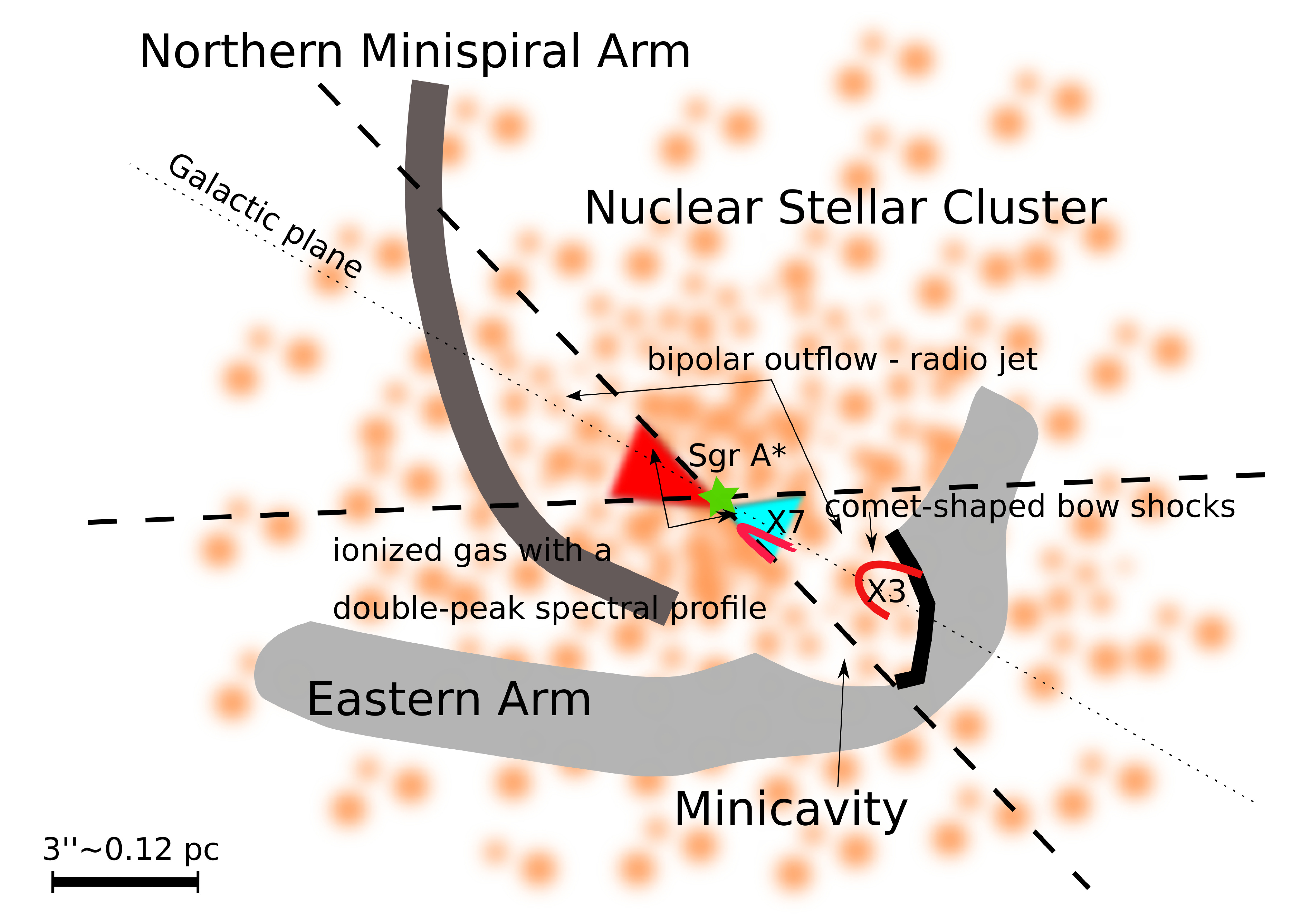
Figure 27: An illustration of the orientation of a bipolar outflow – a radio jet with respect to the Galactic plane and other structures in the Galactic center according to Yusef-Zadeh et al., [695]. In particular, we depict the parallel orientation of two prominent bow-shock sources X7 and X3, which are located $\sim 0.8^{\prime\prime}$ and $\sim 3.4^{\prime\prime}$ from Sgr A* in projection, respectively; see also Mužić et al., [469], Peißker et al., [528], Peißker et al., 2021a [524].

Inside the Bondi radius expressed by Eq. (94), the accretion flow towards Sgr A* is currently well-explained in the framework of radiatively-inefficient accretion flows (RIAFs). One of the models of RIAFs is an optically thin advection dominated accretion flow (ADAF), which is characterized by advective cooling in comparison with standard accretion disks (see Chapter 2), which cool efficiently down radiatively. By advective cooling it is understood that the energy released via the flow viscosity is stored as entropy and essentially is transported inward by accretion. If we look at the flow element at the fixed radius from a rest frame, the material with larger entropy moves inward and is replaced by the lower-entropy material from an adjacent outer part of the flow. This way the ADAF flows can be become much hotter than standard thin disks, which leads to high-energy emission. The peak of the spectral energy distribution of Sgr A* hot flow is in the sub-mm/mm domain, which is in contrast with the spectrum of the thin, optically thick disks typical of AGN that peak in the UV domain, which is known as the Big Blue Bump, see also Fig. 2 for comparison. The submm/mm bump of Sgr A* spectrum divides the optically thick part of the spectrum towards lower frequencies and the optically thin part towards the higher frequencies. The optically thin part of the spectrum is characterized by order-of-magnitude flares in the near-infrared (NIR) and the X-ray domains. There are about $\sim 3-5$ flares in the NIR domain, while about one X-ray flare a day. In addition, there is a correlation between the two domains – every X-ray flare has a NIR counterpart, while the opposite is not true, see Witzel et al., [685] for a detailed analysis and multi-wavelength modelling of the flares.

Another property of hot flows is the radial dependency of the accretion rate, $\dot{M}_{\rm in}\approx\dot{M}_{\rm in}(r)$ [694]. In other words, at the Bondi radius, the accretion rate is as large as $\dot{M}_{\rm B}\approx 10^{-3}\,{\rm M_{\odot}\,yr^{-1}}$, while Sgr A* accretes less than $1\%$ of the Bondi rate as inferred from Faraday-rotation measurements [411, 412]. Hence, most of the accreted matter at the Bondi radius is lost via the outflow, which can be collimated and form a bipolar outflow or a radio jet close to the Galactic plane [695]. This outflow can interact with the minispiral streamers, and the minicavity region is speculated to have been formed by the interaction with the nuclear outflow. In addition, there are several comet-shaped stellar bow-shock sources – X7 [469, 524], X3 [469] and X8 [528] – whose axis of symmetry is oriented along the candidate collimated outflow, see also Fig. 27 for the illustration. Alternatively, this outflow could originate from the stellar cluster and not from the accretion flow. Either way, stellar bow shocks are powerful probes of the ambient circumnuclear medium in terms of the ambient-medium flow [578, 697, 302].

2 Accretion onto supermassive black holes

“The key inspiration which determined my future life came with the series of lectures by Bohdan Paczyński. His lectures showed astrophysics as a dynamically developing new branch, with plenty of things to do. This was something completely new, like opening a window and letting in fresh air."

— Bożena Czerny

2.1 Strong gravity and accretion tori

The gravitational field is described by the Kerr metric, which can be written in the well-known Boyer–Lindquist coordinate system $(t,r,\theta,\phi)$ [453, 125]. This spacetime is asymptotically flat and it obeys the axial symmetry about the rotation axis and stationarity with respect to time; the singularity is hidden below the event horizon. The mass $M$ of the black hole is concentrated in the origin of the coordinate system. The spin parameter $a$ of the Kerr metric describes its rotation; the condition about the presence of the outer event horizon at a certain radius, $r=R_{+}$ (where the horizon encompasses the singularity) leads to the maximum value of the dimensionless spin rate: $|a\leq 1|$. The solution can be then written in the form of the metric element [453, 125, 668]

$${\rm d}s^{2}=-\frac{\Delta\Sigma}{A}\,{\rm d}t^{2}+\frac{\Sigma}{\Delta}\,{\rm d}r^{2}+\Sigma\,{\rm d}\theta^{2}+\frac{A\sin^{2}\theta}{\Sigma}\;\left({\rm d}\phi-\omega\,{\rm d}t\right)^{2},$$ (95)

where $\Delta(r)=r^{2}-2r+a^{2}$, $\Sigma(r,\theta)=r^{2}+a^{2}\cos^{2}\theta$, $A(r,\theta)=(r^{2}+a^{2})^{2}-{\Delta}a^{2}\sin^{2}\theta$, $\omega(r,\theta)=2ar/A(r,\theta)$ (geometrical units are assumed with the speed of light $c$ and gravitational constant $G$ set to unity).

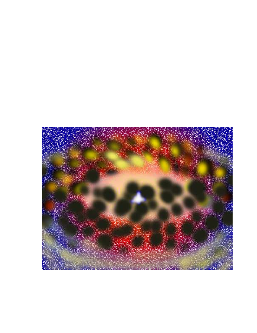
Figure 28: An illustration of an active galactic nucleus. The main components of the system are shown: the supermassive black hole is hidden within the bright accretion region in the centre, surrounded by orbiting clouds and stars. The origin of clouds is probably due to disruption of the accretion torus by instabilities; they are irradiated from the centre and the primary X-rays are reprocessed on the clouds surfaces. The intrinsic spectrum is determined mainly by the Comptonization, depending sensitively on the ionization level. An almost clean line of sight to the central source temporarily emerges. This illustration has been adapted from Karas et al., [322].

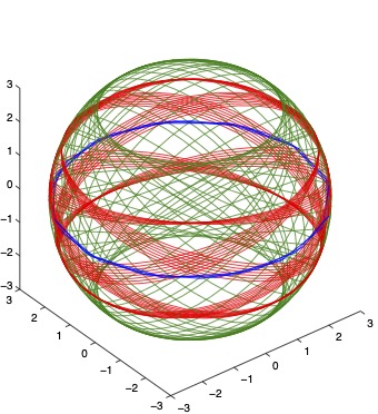
Figure 29: Example of three spherical orbits of free particles moving along different inclination angles near a rapidly spinning Kerr black hole in the center of the coordinate system. Axes are labeled with dimensionless length units of $GM/c^{2}$; the blue circular trajectory resides in the equatorial plane (the plot was drawn by Ondřej Kopáček).

Despite the fact that the Kerr metric is only axially symmetric (it does not obey spherical symmetry unless $a=0$) it is interesting to note that free spherical $R={\rm const}$ orbits are possible with the radius above the ISCO at an arbitrary inclination with respect to the equatorial plane (even residing within the polar plane) as shown in Fig. 29 [678, 637].

The plasma forms an accretion disk or a torus residing in the equatorial plane, so that the axial symmetry is maintained on the overall scale (Fig. 28). In a non-magnetized (purely hydrodynamical) limiting case one can find the classical solution for the density distribution $\rho\equiv\rho(r,z)$ and pressure $P\equiv P(r,z)$, and geometrical shape $H\equiv H(r)$ of a non-gravitating polytropic torus, $P=K\rho^{k}$ [4, 5]. Introducing enthalpy of the medium, $W(P)\equiv\int dP/\rho.$ By setting $P_{\rm in}=P_{\rm out}=0$ at the inner and the outer edges of the density distribution, Abramowicz et al., [5] find

$$W_{\rm out}-W_{\rm in}=\int_{R_{\rm in}}^{R_{\rm out}}\,\frac{l(R)^{2}-l_{\rm kep}(R)^{2}}{R^{3}}\,dR=0,$$ (96)

where $l_{\rm kep}(R)$ is the radial profile of the Keplerian angular momentum density in the equatorial plane. Several properties of this solution are worth mentioning [122, 662]: (i) The level surfaces of functions $P,$ $\rho,$ and $W$ coincide; (ii) If the torus boundary $P=0$ forms a closed surface, the torus center is defined by where $dP/dR=0,$ the pressure is maximum; (iii) The shape of the torus can be found by integrating the vertical component of the Euler equation (Fig. 30).

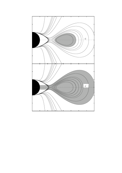
Figure 30: Schematic sketch of meridional sections across the equipotential surfaces $W={\rm const}$. Possible shapes are shown of non-magnetized polytropic tori with constant angular momentum density ($k=4/3$, $l={\rm const})$ near a black hole (denoted by black circle). The fluid can overflow over the critical, self-crossing surface C (dashed line). Top panel: all material is confined within a closed, stable configuration; bottom panel: accretion of material overflowing across the critical surface.

Above a certain critical value, $W>W_{c},$ the torus forms a stable configuration (see the shaded region), while for $W<W_{c}$ matter overflows onto the central object even if we neglect viscosity. This behaviour resembles the Roche lobe overflow in binary systems, however, here it is a consequence of the non-monotonic radial dependence of the Keplerian angular momentum in the relativistic regime near the black hole. Whereas the material inflowing from the atmosphere of a primary component of the binary system concentrates near the equatorial plane and naturally forms the torus, in the case of a single, isolated central black hole matching the inner (toroidal) structure to the outer reservoir of matter depends on many circumstances at the outer boundary region. This is also the case of supermassive black holes residing in nuclei of galaxies, which are fed by the interstellar medium from a surrounding (spheroidal) nuclear star cluster and the galaxy bulge; flattening of the structure is a parameter that can vary from disk-type equatorial inflow up to perfectly spherical (Bondi-type) solution [608] at large radius. Let us note that the assumptions about constancy of $l(R)$ (angular momentum density along von Zeipel cylinders) and vanishing magnetization in Fig. 30 are astrophysically unrealistic but they are useful to simplify calculations and allow an analytical insight.

Even in the case of a strongly magnetized environment the contribution of an astrophysically realistic magnetic energy to the space-time curvature is negligible. We can thus neglect its effect on the metric terms and assume a weak-field limit on the background of the Kerr black hole. In order to initiate the numerical code, we can employ an initially uniform magnetic field [667], which is described completely by two non-vanishing components of the four-potential,

$$A_{t} = Ba\Big{[}r\Sigma^{-1}\left(1+\cos^{2}\theta\right)-1\Big{]},$$ (97)

$$A_{\phi} = B\Big{[}{\textstyle\frac{1}{2}}\big{(}r^{2}+a^{2}\big{)}-a^{2}r\Sigma^{-1}\big{(}1+\cos^{2}\theta\big{)}\Big{]}\sin^{2}\theta,$$ (98)

in dimensionless Boyer–Lindquist coordinates and $B$ is the magnetic intensity of the uniform field far from the event horizon. The magnetic field and the associated electric component are generated by currents flowing in the accreted medium far from the black hole, as the latter does not support its own magnetic field (for further discussion, see below in the text). The set of two non-vanishing four-potential vector components defines the structure of the electromagnetic tensor, $F_{\mu\nu}\equiv A_{[\mu,\nu]}$; by projecting onto a local observer frame, one then obtains the electric and magnetic vectors. However idealized the initial configuration may be, the numerical solution rapidly evolves in a complex entangled structure, with field lines turbulent within the accreting medium and more organized in the empty funnels that develop outside the fluid structure.

2.2 Main components of the radiation spectrum from black hole accretion

The AGN SED differs from normal galaxies mainly by the large luminosity across the electromagnetic spectrum from radio to gamma-rays, both extreme long and short wavelengths being present particularly when the AGN produces significant emission from the outflowing, relativistically fast jet. The large AGN luminosity (typical AGN luminosity is by more than eight orders of magnitude larger than the luminosity of Sgr A* in our Galactic centre) can be well explained by accretion onto a supermassive black hole. Depending on the accretion mode (see the chapter 4 for more details), the total emission is either dominated by thermal emission from an accretion disk or by non-thermal emission from the accretion disk corona and/or relativistic jet.

Accretion disk thermal emission

The thermal blackbody radiation is described by the Planck radiation law. The spontaneous radiative distribution of the entropy emerges radiation with the specific intensity $B$  [W m^-2 Hz^-1 sr^-1], given by the Planck function:

$$B(\nu,T)=\frac{2h\nu^{3}}{c^{2}}\frac{1}{{\rm e}^{\frac{h\nu}{kT}}-1},$$ (99)

where $\nu$ is the emitted frequency and $T$ is the temperature of the blackbody surface. The blackbody emission is radiated by an optically thick matter, in which the thermal photons emerge multiple scattering with particles and the temperature possesses a value corresponding to the kinetic energy of the particles.

The peak frequency $\nu_{\rm peak}$ is the frequency at which $B(\nu,T)$ given by Eq. (99) reaches its maximum. It is proportional to the temperature:

$$h\nu_{\rm peak}=2.82kT,$$ (100)

which was known before the Planck’s law as the Wien displacement law. For frequencies well below the peak, its course is well described by:

$$B(\nu,T)\approx\frac{2\nu^{2}kT}{c^{2}}\quad\mbox{(Rayleigh--Jeans's law)},$$ (101)

and for frequencies well above the peak by:

$$B(\nu,T)\approx\frac{2h\nu^{3}}{c^{2}}{\rm e}^{-\frac{h\nu}{kT}}\quad\mbox{\rm(Wien's law)}.$$ (102)

It is straightforward to derive both, the Rayleigh–Jeans’s approximations from Eq. (99) by the Taylor expansion ${\rm e}^{\frac{h\nu}{kT}}=1+\frac{h\nu}{kT}+\cdots$ (and the Wien’s approximation by neglecting unity against the exponential in the denominator of Planck’s law).

The energy flux of blackbody radiation is given by

$$F=\sigma T^{4}\quad\mbox{Stefan--Boltzmann's law},$$ (103)

where $\sigma$ is the Stefan–Boltzmann constant $\sigma=\frac{2\pi^{5}k^{4}}{15c^{2}h^{3}}$.

An accretion disk does not emit blackbody radiation with a single temperature. The temperature at each position is determined by the particle’s kinetic energy. This energy decreases with the radius and thus also the temperature drops. The radial dependence of the temperature for the accretion disk surface around a black hole can be determined by Shakura and Sunyaev, [599] standard-disk scenario:

$$T(r)=\left(\frac{3GM\dot{M}}{8\pi\sigma r^{3}}\left[1-\left(\frac{r_{\rm in}}{r}\right)^{\frac{1}{2}}\right]\right)^{\frac{1}{4}},$$ (104)

where $r_{\rm in}$ is the inner edge of the disk.

The total thermal emission from an accretion disk is the composition of contribution from multiple radii with different surface temperatures, known as the multicolor blackbody emission. This multicolor blackbody was successfully applied to thermal X-ray spectra of X-ray binaries [454], confirming the general validity of the temperature radial dependence given by Eq. 104. More sensitive X-ray data have later revealed deviation from the perfect blackbody emission, mostly caused by the Comptonization of thermal photons in the upper layers of the accretion disk [154, 569, 605]. Taking into account the vertical structure of the disk leads to the spectral hardening and the local specific flux is diluted blackbody emission:

$$F_{\nu}=\frac{\pi}{f^{4}_{\rm col}}B_{\nu}(f_{\rm col},T_{\rm eff}),$$ (105)

where $B_{\nu}$ is the Planck function (Eq. 99), $T_{\rm eff}$ is the effective temperature, and $f_{\rm col}$ is the hardening factor. The value of the hardening factor is a function of the accretion rate and may vary depending on the accretion state [see, e.g. 168].

Equation (104) can be re-written to have a useful formula for estimating the temperature of accretion disks around black holes with various mass or accretion rate in terms of Eddington units:

$$T\left(\frac{r}{R_{g}}\right)\approx 6.3\times 10^{5}\,{\textnormal{K}}\left({\frac{M}{10^{8}M_{\odot}}}\right)^{-\frac{1}{4}}\left(\frac{\dot{M}}{\dot{M}_{\rm Edd}}\right)^{\frac{1}{4}}\left(\frac{r}{R_{g}}\right)^{-\frac{3}{4}}f(r),$$ (106)

where $R_{g}$ is the gravitational radius (defined by Eq. 18), and $f(r)=\left[1-\left(\frac{r_{\rm in}}{r}\right)^{\frac{1}{2}}\right]^{\frac{1}{4}}$. For the same accretion rate in Eddington units and the inner edge of the disk, the temperature scales with mass as:

$$T\propto M^{-\frac{1}{4}}.$$ (107)

Note that Eq. 107 is valid when the accretion rate is expressed in units of Eddington values, otherwise the temperature would be $T\approx M^{-\frac{1}{2}}\dot{M}^{\frac{1}{4}}$. However, for comparison of accreting black holes of different mass but with a similar Eddington ratio, Eq. 107, is the most useful and we can immediately estimate where the peak of AGN thermal emission should be based on the knowledge of measured accretion disk temperatures in X-ray spectra of XRB. The thermal emission of accretion disks in AGN thus peaks in the UV range ($T\approx 10^{5}$ K), while the temperature peak occurs at the soft X-ray band for stellar-mass black holes in X-ray binaries ($T\approx 10^{7}$ K).

The observed spectrum of AGN has indeed typically a peak in the UV band, the big blue bump [567]. Some UV spectra of quasars can be well fitted by the thermal disk emission [156], but it is not the case in general [211]. The UV and especially the range between far-UV and X-rays is heavily affected by the interstellar absorption, preventing astronomers from a detailed study of spectral properties of the thermal accretion disk emission in AGN.

Thermal bremsstrahlung radiation

Thermal bremsstrahlung is radiated in a hot plasma due to the Coulomb collisions of the ions. The electrons are accelerated by the collisions to high velocities and emit radiation that can escape the plasma if it is optically thin. Therefore, the AGN corona produces not only up-scattered emission from the accretion disk but also its own thermal emission. This is, however, very different from the thermal emission of the blackbody emission of the optically-thick accretion disk and is, therefore, sometimes not accurately referred to as a non-thermal component of AGN.

The temperature of the plasma is defined by the ion velocities, which have in thermal equilibrium the Maxwell–Boltzmann distribution. The temperature is proportional to the average kinetic energy of ions:

$$\frac{3}{2}kT=\left<\frac{1}{2}mv^{2}\right>,$$ (108)

where $m$ and $v$ are the ion mass and the thermal speed, respectively. In the thermal equilibrium, the average kinetic energy is equal for ions and electrons. Therefore, the ions can be considered stationary with respect to the fast moving electrons. Different situations can happen in the collisions. The free-free transition occurs when the electron freely passes near the ion and is not kept. Such radiation yields the continuum spectrum without lines, and is called bremsstrahlung.

The radiated power per unit photon energy and per unit volume is given by:

$$\epsilon_{\rm free-free}=2\sqrt{\frac{2}{3\pi}}\,n_{e}\,n_{i}\,\alpha\,\sigma_{T}\,c\,Z^{2}\,\Theta^{-1/2}\,g(\Theta,E)\,e^{-E/kT},$$ (109)

where $n_{i}$ is the ion density, $n_{e}$ is the electron density, $\alpha$ is the fine structure constant, $Z$ is the effective charge of the ion, $\Theta\equiv k_{B}T/m_{e}c^{2}$, and $g$ is the Gaunt factor, which is a dimensionless quantity of order of 1 and slightly changes with the spectral energy (frequency).

When the electron is captured by the ion and fills one of the ion vacancies, the transition is free-bound and the continuum emission is associated also with spectral-line emission corresponding to the transition. The process of free-bound transition is called radiative recombination. How often the ionization and recombination of atoms is happening depends mainly on the plasma density but also on the nature of equilibrium. More recombinations occur at the photoionization equilibrium than in the collisional ionization equilibrium since the temperature at the photoionization equilibrium is lower for comparable ionization.

Figure 31: Left: a schematic picture of the main radiation components of an accreting black hole: thermal radiation from the accretion disk, up-scattered in a hot corona and reflection emission. Light rays are distorted by strong gravity of the central black hole. Right: a schematic view of the inverse Compton effect in the local frame frame where electrons have energy high enough compared to the ambient light, so the mechanism up-scatters the ambient photons.

Non-thermal AGN emission

The thermal emission of AGN accretion disks contributes mainly to the UV domain, but AGN are very bright X-ray sources as well and the thermal bremsstrahlung of the corona is not sufficient to produce the observed X-ray intensity. The X-ray emission can be, therefore, best explained by scattering of the thermal emission in the corona, as illustrated in Figure 31. The very high temperature causes that the electrons in the corona possess very high velocities. Their kinetic energy is partly transported to the low-energy photons scattering on the electrons, and the photons thus gain energy and increase their frequencies. The resulting radiation dominates in X-rays, more energetic than UV. This effect is known as the inverse Compton scattering. Further, we will show that this effect can be understood in terms of the special-relativistic transformation in relations for Compton scattering.

The initial and final energy of a photon can be written in the units of electron rest energy:

$$e_{i}=\dfrac{h\nu_{i}}{m_{e}c^{2}}\;,\qquad e_{f}=\dfrac{h\nu_{f}}{m_{e}c^{2}}\;,$$ (110)

where $m_{e}$ is the mass of electron, $h$ is the Planck constant, and $\nu_{i}$, $\nu_{f}$ are the initial (before collision) and final (after collision) frequencies of photon, respectively. Based on the law of energy and momentum conservation, the final energy of the photon after the Compton scattering is:

$$e_{f}=\dfrac{e_{i}}{1+e_{i}\Lambda}\;,$$ (111)

where $\Lambda=1-\cos{\vartheta}$ and $\vartheta$ being an angle between the direction of photon before and after the collision. The final frequency of the photon can be obtained by multiplying the equation (111) by factor $m_{e}c^{2}$:

$$\nu_{f}=\dfrac{m_{e}c^{2}\nu_{i}}{m_{e}c^{2}+h\nu_{i}\Lambda}\;.$$ (112)

Equations (111) and (112) are valid in the electron rest frame. But now, let us assume that the electron is in the relativistic regime with the Lorentz factor $\gamma=\frac{1}{\sqrt{1-v^{2}/c^{2}}}=\frac{1}{\sqrt{1-\beta^{2}}}$, and rewrite the equation for Compton scattering in the laboratory frame. We further denote laboratory frame by an index "L" and the rest frame by an index "R". The final energy of the photon in the laboratory frame can be written as:

$$e^{L}_{f}=e^{R}_{f}\gamma\left(1+\beta\mu^{R}_{f}\right),$$ (113)

where $\mu=\cos{\chi}$ and $\chi$ is the angle between the direction of electron and photon before the collision. Using Eq. 111, we get:

$$e^{L}_{f}=\dfrac{e^{R}_{i}}{1+e^{R}_{i}\Lambda^{R}}\gamma\left(1+\beta\mu^{R}_{f}\right)$$ (114)

Using transformations $\dfrac{1}{\gamma}\dfrac{1}{1-\beta\mu^{L}_{f}}=\gamma\left(1+\beta\mu^{R}_{f}\right)$ and $e^{R}_{i}=e^{L}_{i}\gamma\left(1-\beta\mu^{L}_{i}\right)$, we get a formula for the final energy of the photon in the laboratory frame as:

$$e^{L}_{f}=e^{L}_{i}\,\dfrac{1-\beta\mu^{L}_{i}}{1-\beta\mu^{L}_{f}}\,\dfrac{1}{1+e^{L}_{i}\gamma\left(1-\beta\mu^{L}_{i}\right)\Lambda^{R}}\;.$$ (115)

Assuming photons with a low initial energy, so that the condition $\gamma e^{L}_{i}\ll 1$ is fulfilled, the equation can be simplified to:

$$e^{L}_{f}\approx e^{L}_{i}\,\dfrac{1-\beta\mu^{L}_{i}}{1-\beta\mu^{L}_{f}}\;,$$ (116)

which can be rewritten to:

$$e^{L}_{f}\approx e^{L}_{i}\gamma^{2}\left(1-\beta\mu^{L}_{f}\right)\left(1+\beta\mu^{R}_{f}\right).$$ (117)

From the last equation, it follows that the final energy of the photon in the laboratory frame must be larger than the initial energy and lower than the product of the initial energy and a factor of 4$\gamma^{2}$ that is larger than 1 and is the higher the higher velocity of electron is:

$$e^{L}_{i}~{}\lesssim~{}e^{L}_{f}~{}\lesssim~{}4\gamma^{2}e^{L}_{i}\;.$$ (118)

Other source of the AGN non-thermal emission is the synchrotron emission from the relativistic jets. The synchrotron emission comes from the accelerated electrons in the magnetic field. Its power (in the observer’s frame) increases with the second power of electron’s energy and magnetic-field intensity. Therefore, it is strong especially in the black-hole jets where the electrons are highly relativistic (see Chapter 3). This causes a strong beaming effect and most of the energy is radiated into a narrow beam. Therefore, the synchrotron emission is the most dominant radiation component in blazars, i.e. in AGN with strong jets pointing towards us, while it is negligible for radio-quiet AGN. We refer to standard books, Rybicki and Lightman, [e.g., 575], to read more about different mechanisms of thermal and non-thermal radiation.

Another important component of the AGN emission is reprocessing of the primary radiation. This happens very close to the black hole in the accretion disk, as it is illustrated in Fig. 31 (left panel), as well as at more distant structures, such as AGN tori. The reprocessing at tori usually produce a large fraction of infrared emission because the AGN radiation heats the dust there. The reflection at the innermost disk is particularly interesting in the X-ray domain, because the reprocessed emission there can even overcome the primary radiation that is declining at high energies. The most prominent features of the innermost X-ray reflection are the broad iron line and the Compton hump. These spectral features can be used to derive the basic parameter of the central black hole, its angular momentum (spin), as it is shown in the next chapter.

Figure 32: A computer-generated image of a black hole accretion disk, as seen by a distant observer at $\theta_{\rm inc}=80$ degree inclination view angle [107]. A black hole shadow develops in the central part of the image, surrounded by a set of narrow rings of photons encircling the black hole along indirect, highly bent rays.

Strong-gravity effects in radiation signal from accretion disk

Accretion disks may be seen as axially symmetric and stationary at the zero approximation. However, a variety of non-axisymmetric perturbations are known to develop, grow and influence their structure. This leads to the fluctuating observed signal with characteristic imprints of the black hole strong gravity in continuum and spectral-lines [235, 338]. Relativistic effects can be described within the geometrical optics, where photons follow null geodesics towards a distant observer. The radius of the emission site and the viewing angle (inclination) of the observer with respect to the disk plane are the main parameters for the signal arising near the inner edge, supplemented by the black-hole spin [217, 324]. These imprints can be characterized in several steps.

Each pixel within the detector plane corresponds to a photon ray arriving from the source, namely, the accretion disk surface $z\equiv z(R)$. Photon trajectories are not straight lines in space, leading to a distorted image (Fig. 32). Radiation intensity transforms from the local disk frame, $I^{\rm R}(R,z(R);\,$$\nu^{\rm R},\mu^{\rm R}),$ to the observer’s (laboratory) frame, $I^{\rm L}(R,z(R);\,$$\nu^{\rm L},\mu^{\rm L})$, and propagates to the detector plane (here, $\mu$ is the directional cosine of the emerging photon measured from the normal to the disk surface.).

The gravitational field of the central object and the disk modify the shape of spectral features coming from the disk [152, 151, 375]; this is apparent especially at high view angles and with fast-rotating black hole, where photons experience large line-of-sight velocity and the radiation is produced mostly at very small radii near the black hole. Finally, Laor and Netzer, [378] studied continuum spectra produced by self-gravitating disks, whereas Karas et al., [329], Schee, [582], and Usui et al., [649] calculated the predicted profiles of spectral lines within the framework of exact general-relativistic solutions. These approaches give an improved (consistent) picture where the matter of the accretion flow generates radiation and, at the same time, the accretion disk mass modifies its internal structure and acts back on the emerging photon rays as they travel toward the observer.

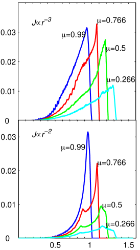
Figure 33: Left panel: contour lines of three governing functions in the equatorial disk plane $(r,\phi)$ that determine effects of strong gravity of the central black hole onto observed radiation from a Keplerian disk: (i) the overall (Doppler and gravitational) energy shift $g(R,\phi)$ (red); (ii) local emission angle (in degrees) with respect to disk, affected by the relativistic aberration (green); (iii) time-delay (in geometrized units) due to light travel time from the disk plane to the distant observer located at large radius. Parameters of the plot: view angle $\theta_{\rm inc}=60$ deg, spin $a/M=0$ (Schwarzschild black hole – the black circle). The grid extends up to $70GM_{\bullet}/c^{2}$; ISCO radius $R_{\rm ms}=6GM_{\bullet}/c^{2}$ (yellow circle). Right panel: the resulting (computed) profiles of the relativistic spectral line. Effect of the overall broadening and skewness are apparent (more profoundly for edge-on view angles). Different power-law radial profiles of the intrinsic emissivity $J(r)\propto r^{-n}$ have been laid on the accretion disk with several view angles $\mu\equiv\cos\theta_{\rm inc}$. Energy on the horizontal axis is normalized to the line intrinsic energy; the radiation flux on the vertical axis is in arbitrary units. For a direct comparison with previous papers we selected the case of a rapidly rotating Kerr black hole $a/M=0.998$ and an accretion disk extending from the innermost stable circular orbit [ISCO; other parameters as in 375].

In order to reveal the spectral profile, we calculate the total observed flux of radiation by collecting photons,

$$F^{\rm L}(\nu^{\rm L})_{\mid\theta=\theta_{\rm obs}}=\int_{\lower 3.0pt\hbox{\footnotesize(Over observer's plane)}}I^{\rm L}(\nu^{\rm L})_{\mid R\rightarrow\infty,\theta=\theta_{\rm obs}}\,dS.$$ (119)

A typical double-horn skewed profile arises in the observed spectral line [219, 415, 414].

Doppler factor, $g\equiv g(r;a/M,\theta_{\rm inc})\,\equiv\,1+z=E_{\rm obs}/E_{\rm em}$, characterizes the redshift function $z$ between the emitted (subscript “”em”) and observed (“obs”) of photons originating at different sides of the source (increase of the energy at the approaching side, and vice versa at the receding side of the disk). This relates to the change of radiation intensity by the corresponding factor $g^{3}$. The effect tends to enlarge the width of the spectral features and to enhance the observed flux at its high-energy tail. In addition to the special-relativistic effect, the overall gravitational redshift of General Relativity contributes to the $g$-factor and affects mainly photons coming from the inner parts of the source in the deep potential well. Finally, the gravitational lensing enhances the emerging flux from the far side, i.e., the section of the accretion disk at the upper conjunction with the black hole; this leads to the enhancement of the observed flux around the centroid energy (see Fig. 33).

Let us remind the reader that the central (Kerr) black hole is assumed to be the only source of gravitational field in and there are no secondary bodies influencing gravitationally the inner disk. This may not be true in the case of binary SMBHs that can warp the disk; furthermore, an alternative description of gravity, if viable, could modify the standard picture described here.

Light rays of the geometrical optics approximation are determined by Maxwell’s equations for the electromagnetic field tensor. In the vacuum we can write

$${F^{\mu\nu}}_{\!;\nu}=0,\quad{{}^{\star}F^{\mu\nu}}_{\!;\nu}=0,$$ (120)

where the asterisk denotes a dual tensor. The associated electric field components are projections onto observer’s four-velocity, $E^{\alpha}=F^{\alpha\beta}u_{\beta}$, and an electromagnetic wave is defined as a solution of the form

$$F_{\alpha\beta}=\Re e\left[u_{\alpha\beta}\;e^{\Im\psi(x)}\right].$$ (121)

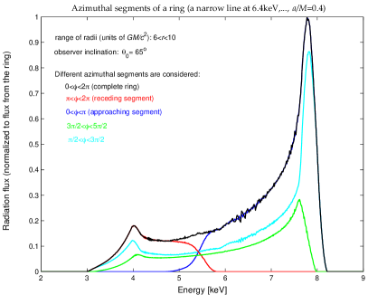
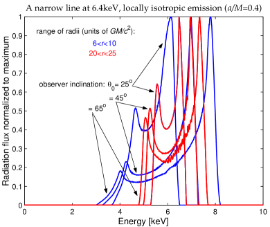
Figure 34: Explaining the formation of relativistic spectral line profiles originating from a range of radii within a geometrically thin, planar, Keplerian accretion disk that resides in the equatorial plane of a moderately spinning Kerr black hole ($a/M_{\bullet}=0.4$). Left panel: intrinsically, the line has a narrow ($\delta$-type) profile centered around the rest-frame energy $6.4$ keV. The composite profile (black) consists of contributions from four azimuthal segments in the disk, as indicated by different components and described in the figure legend. The approaching side of the disk creates the amplified high-energy wing (blue), whereas the receding part is weaker and shifted toward the less energetic part of the spectrum (red). Right panel: Examples of the line profile broadening that arises from different radii and observer inclinations, as indicated within the plot.

Two scales are introduced at this point. The phase $\psi(x)$ is a a rapidly varying function, while the amplitudes $u_{\alpha\beta}$ vary slowly. We can thus define a wave vector, $k_{\alpha}\equiv\psi_{,\alpha}$, which obeys parallel transported along the null geodesics, $k_{\alpha;\beta}\,k^{\beta}=0$, $k_{\alpha}k^{\alpha}=0$. The propagation law in the empty curved spacetime thus reads [202, 207]

$$DF_{\alpha\beta}-2\theta F_{\alpha\beta}=0,$$ (122)

where $\theta\equiv-\frac{1}{2}{k^{\alpha}}_{;\alpha}$ describes the expansion of null congruences, $D\,\equiv\,u^{\alpha}\nabla_{\alpha}$. Superposition of the above-described influences is modeled and explained with Fig. 34–35, where we show the dependence of the predicted profiles on the parameters in comparison with simulations in the original works [375, 352, 334]; we notice an excellent agreement and give the values that can be useful especially for tests of new numerical codes. Furthermore, in Figs. 36–37 we explore dynamical spectrum expected to be seen from an orbiting spot or a similar kind of a feature of enhanced emission on the accretion disk surface; time resolution offers a significant improvement to constrain the line-producing region but the observation requires much longer duration and sensitivity to capture enough photons.

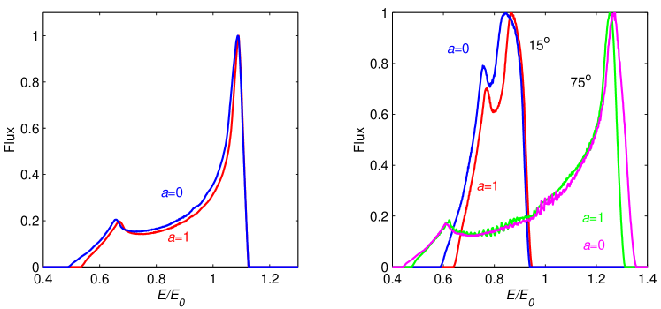
Figure 35: The dependence on the black hole spin and the inclination angle for the predicted profiles from a ring extending between ($6$–$10)\,GM/c^{2}$ [other parameters as in 352].

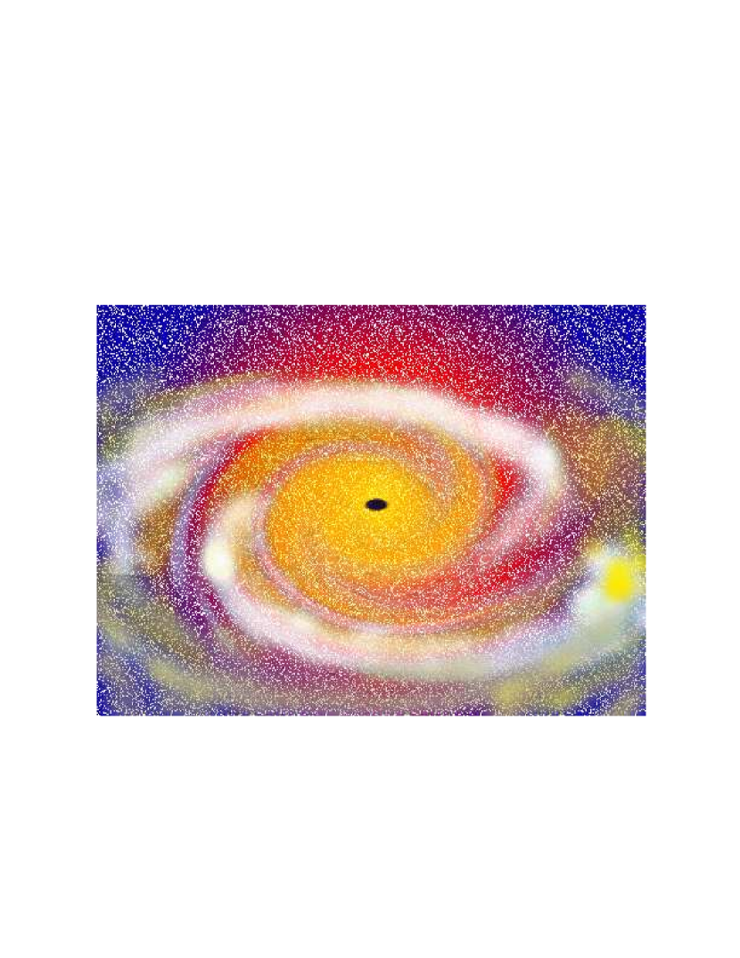
Figure 36: An artistic sketch of spiral patterns on an accretion disk as another physically motivated origin of quasi-periodic modulation of the incoming radiation signal. Spiral-wave structures produce a rich variety of spectra and light curves, broader than what we can explain with the help of strictly localized spots. This scheme is complementary to the idea of instant off-axis flares inducing the observed line variations and it enables us to restrict the geometry of the source by means of the reverberation technique. Figure adopted from Karas et al., [330].

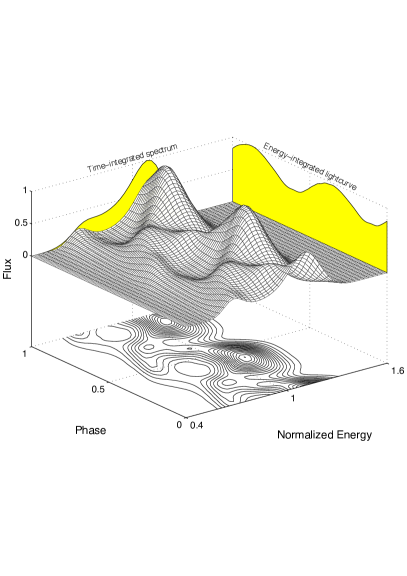
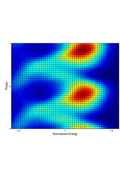
Figure 37: A time-dependent model spectrum produced by a non-axisymmetric pattern (spiral wave) orbiting within a black hole accretion disk. Left panel shows the predicted radiation as detected by a distant observer (moderate inclination angle $\theta_{\rm inc}=50$ deg). The energy-integrated light curve and time-integrated spectrum are shown as projections of the full dynamical spectrum. In a typical situation of an AGN accretion disk, and especially for small radii and intermediate to large inclination angles, most of the line emission arises from only a small fraction of the orbit. Right panel: observed energy of the spectral line vs. orbital phase of the pattern. The color scale of the diagram encodes different levels of the observed flux (red corresponding to the maximum enhancement, blue the minimum flux; Karas, 2006). This can be compared with an early evidence in Iwasawa et al., [310].

Let us make an obvious but important remark, notably, that the above-mentioned idealized scheme must become more complex in realistic astrophysical circumstances. This leads to additional degrees of freedom of the system and causes some kind of degeneracy between parameters (they cannot be constrained in a unique way, instead, the best-fit procedure can find during the minimization process different local minims). Hence, one needs more accurate observations and improved signal-to-noise resolution in order to constrain the models. This complication is demonstrated in Fig. 38, where we plot exemplary profiles of a spectral line influenced by additional diverse effects, including the self-gravity, which have been ignored in previous models [649]. Likewise, a geometrically thick (flaring) vertical profile of the accretion disk surface and/or the presence of warps need to be taken into account especially at higher luminosity [162, 636], but these have been neglected in the past mainly for the sake of simplicity of calculations.

Figure 38: Examples of synthetic emission-line profiles from an accretion disk, taking into account a variety of relativistic effects (Doppler and a gravitational shift of frequency, lensing of the observed radiation flux due to gravity of the central black hole) as well as the self-gravity of the accretion disk. The latter influence should be taken into account in realistic models of AGN spectra (in case of the fluorescent iron line in the X-ray domain) because it must inevitably be present. The disk material orbits at a speed that is different from the Keplerian velocity due to self-gravity of the disk matter. Different curves illustrate effects of the black-hole rotation $a/M_{\bullet}$, observer’s inclination $\theta_{\rm inc}$, and different disk models (typically, $M_{\rm disk}/M_{\bullet}\approx 10^{-2})$. The inclination angle varies over different panels from a small value (pole-on view – top left, narrow line) up to $\theta_{\rm inc}\simeq 80$ deg (almost edge-on view – bottom right, relativistically broadened and skewed profiles). In each panel, contributions from different radial regions of the disk are indicated by different line styles, while the total flux from the entire disk is plotted by the solid line (background subtracted and normalized to the maximum). Figure adapted from Karas et al., [329].

In the presence of a refractive and dispersive media the approach of relativistic geometric optics in curved spacetimes was extended [20, 70] and then implemented numerically for practical computations [e.g. 541]. The effects of gravitational lensing in the curved spacetimes combine with refraction as light rays propagate through the medium. Kinch et al., [345] have matched general relativistic magnetohydrodynamic (GRMHD) simulations with a Monte Carlo radiation transport code; this allows the authors to determine the X-ray flux irradiating the disk surface and the coronal electron temperature self-consistently, leading to self-consistent predictions for the relativistic Fe K$\alpha$ spectral profiles. Having in mind the applications to present-day X-ray observations, the energy shifts, gravitational lensing and time delays are the principal effects which originate from general relativity and can be currently tested with data that are in our disposal. Polarimetric information is more complete [556] and the relevant technology is available, however, it reaches beyond capabilities of present observational instruments available in the orbit [58].

The relativistic polarization tensor is defined as $J_{\alpha\beta\gamma\delta}\,\equiv\,\frac{1}{2}\langle F_{\alpha\beta}F_{\gamma\delta}\rangle$, and its projections $J_{\alpha\beta}=J_{\alpha\beta\gamma\delta}\,u^{\gamma}\,u^{\delta}=\langle E_{\alpha}\bar{E}_{\beta}\rangle$ are introduced. Four parameters $S_{A}$ are then given by $S_{\!{}_{A}}\equiv\frac{1}{2}(k_{\alpha}u^{\alpha})^{2}F_{\!{}_{A}}$, where $F_{\!{}_{A}}$ $(A=0,\,\ldots\,3)$ are constructed by projecting the polarization tensor [21]. These quantities satisfy the relations $J_{\alpha\beta}u^{\beta}=0$, $J_{\alpha\beta}k^{\beta}=0$, $\omega=u_{\alpha}k^{\alpha}$ and can be connected with the traditional definition of the Stokes parameters [94, 123].

The normalized Stokes parameters are defined $s_{1}\,\equiv\,S_{1}/S_{0}$, $s_{2}\,\equiv\,S_{2}/S_{0}$, and $s_{3}\,\equiv\,S_{3}/S_{0}$. The degree of linear and of circular polarization is $\Pi_{l}=\sqrt{s_{1}^{2}+s_{2}^{2}}$, $\Pi_{c}=|s_{3}|$, and the total degree of polarization $\Pi=\sqrt{\Pi_{l}^{2}+\Pi_{c}^{2}}$. By propagation through an arbitrary, curved (but empty) spacetime, the radiation flux obeys the relation, $F_{\!{}_{A,\,\rm em}}\,dS_{{}_{\rm em}}=F_{\!{}_{A,\,\rm obs}}\,dS_{{}_{\rm obs}}$ from which the redshift $z$ relates the photon energy at a point of emission with that at a distant observer,

$$1+z=\frac{(k_{\alpha}u_{\alpha})_{\rm em}}{(k_{\alpha}u_{\alpha})_{\rm obs}},\quad S_{\!{}_{A}}=\frac{k_{\!{}_{A}}}{(1+z)^{2}dS}.$$ (123)

For example, in the case of a thin rotating disk near Kerr black hole, the redshift factor $z$ and the local emission angle $\vartheta$ are given by

$$1+z=\frac{r^{3/2}-3r^{1/2}+2a}{r^{3/2}+{a}-\xi},\quad\cos\vartheta=\frac{g\eta^{1/2}}{r};$$ (124)

$\xi$ and $\eta$ are constants of motion.

The gravitational field of a Kerr black hole (95) can be written in the form [453]

$$ds^{2}=-\frac{\Delta}{\Sigma}\Big{(}dt-a\sin^{2}\theta\,d\phi\Big{)}^{2}+\frac{\Sigma}{\Delta}\,dr^{2}+\Sigma\;d\theta^{2}+\frac{\sin^{2}\theta}{\Sigma}\Big{[}a\,dt\!-\!\big{(}r^{2}+a^{2}\big{)}\,d\phi\Big{]}^{2}$$ (125)

in Boyer–Lindquist spheroidal coordinates, where $\Delta(r)$ and $\Sigma(r,\theta)$ are known functions. The horizon occurs at $\Delta(r)=0$. Assuming sub-maximal rotation, $|a|\leq 1$, the outer radius is found at the dimension-less radius $r=1+(1-a^{2})^{1/2}$ and it hides the singularity from a distant observer. As a purely GR effect, as soon as $a\neq 0$, all particles and photons are dragged by the rotation of the black hole (the frame-dragging effect).

Eq. (123) shows that the polarization properties of the disk emission are modified by the photon propagation. As the reflecting medium has a disk-like geometry, a substantial amount of linear polarization is expected because of Compton scattering. In order to compute the observable characteristics (i.e., different polarization modes), one has to combine the reflected component with the primary continuum. The polarization degree of the resulting signal depends on the mutual proportion of the different components. Future X-ray satellites will be essential to study GR in the neighbourhood of accreting black holes with outstanding precision, including the polarimetric information.

It is worth noting that the precise shape and variability of the spectral features reflects the intrinsic microphysics of the emitting medium and parameters of the black hole (spin), but it also depends on the gravitational theory that determines the photon propagation. Therefore, this opens a promising way to verify (or reject) the predictions of Einstein’s theory vs. alternative viable theories [for reviews, see 135, 682]. It has been proposed that the detailed features in radiation spectra from accreting black holes and the morphological features shaping the black hole shadows bear tiny signatures that could reveal departures from General Relativity [312, 35, 41, and further references cited therein], although the effects are far too small to be seen at the available resolution of present-day data. In this context an exciting new avenue has been recently opened with the prospects to apply the currently available advanced technology of X-ray polarimetry during the forthcoming decade [715, 676, 613, 364].

2.3 X-ray reprocessing in accretion disk coronae

The X-ray emission produced in AGN is widely accepted to originate via the inverse Compton scattering of thermal UV photons that are scattered in a hot plasma consisting of relativistically moving particles [600, 278, 279]. Such spectrum can be described as a power law from the range $\approx 3\,kT_{\rm bb}$ to $kT_{e}$ [627], where $kT_{\rm bb}$ is thermal black-body emission from the accretion disk and $kT_{e}$ is the electron temperature of the corona. For typical parameters of an AGN super-massive black hole, this range corresponds to energies from a few tens of eV up to a hundred of keV.

It was originally proposed that the AGN corona can originate due to vertically transported heat from the accretion disk by convection [75, 384] or in magnetically confined loop-like structures similar to the observed structure of the solar corona [240]. The major difference between the solar and AGN corona consists in the amount of power that can be released into radiation. While the solar corona contributes to the total flux by less than one percent, the contribution of the X-ray corona in AGN can be any depending on the exact physical and geometrical conditions. The fraction of the corona emission mainly depends on the accretion state that is determined by the accretion rate. Low-accreting sources are accompanied with much stronger corona than highly accreting sources, as seen mainly from the spectral-hardness changes observed in accreting stellar-mass black holes in X-ray binaries [437, 560]. But a similar trend is also observed for AGN. The ratio between the optical and X-ray flux, the $\alpha_{\rm ox}$ parameter, increases with the UV luminosity [616, 394, 442].

Nature and geometry of the X-ray corona

Despite large theoretical and observational attempts in the last decades, the basic questions about the nature and geometry of the corona still remain open. Different heating mechanisms have been proposed from convection of the heat through accretion disk surface to include magnetic reconnection and flares that instantaneously heat the corona. From different considered heating mechanisms, different geometries have been proposed. The corona might be extended, “sandwiching” the disk like its ionized plane-parallel atmosphere [384, 278, 722, 572, 571, 387, 405], or “patchy”, related with the single flares due to magnetic reconnection [240, 176, 159]. Even for the sandwich-structured (also often called as two-phase corona), the importance of the magnetic dissipation of energy as the heating mechanism was noticed [603, 177, 388].

Another often considered geometry of the corona is the so-called “lamp-post” model [416, 415, 185, 489]. This model approximates the corona to be a point-like source above a black hole on its rotational axis. The advantage of this setup is mainly the simplicity of the model that can be used for calculating the spectral shape of the primary as well as the reflected radiation from black hole accretion disk. Thus, it can be easily used for fitting the observed X-ray spectra [184, 165], on contrary to e.g. a patchy corona where many additional parameters would be present. The physical motivation of such a model is that it can well approximate a base of the jet [410] or a collision of shocks in an aborted jet [254], or simply a very compact corona.

The high compactness of the X-ray corona is suggested from X-ray observations. The first indication came from measuring steep radial-emissivity profiles of X-ray reflection spectra of several AGN, such as MCG -6-30-15 [220, 654, 449], 1H0707-495 [222, 720, 679, 167], IRAS 13224-3809 [544], and Mrk 335 [680], as well as X-ray black hole binaries, such as XTE J1650-500 [450], GX 339-4 [446], and Cyg X-1 [221]. The radial emissivity describes the function of the reflection emissivity on the radius from the centre. The measured indices reach values up to $\approx 7$ (i.e. the reflection emissivity $\approx r^{-7}$), which can be hardly explained without requiring a compact X-ray source and strong light-bending effects [629, 166, 185]. Another independent indication of high compactness of the corona comes from the gravitational microlensing of quasars. Recent results from monitoring observations of lensed quasars [126] showed that the X-ray corona can indeed be as small as $30\,R_{g}$. In some cases, such as RXJ 1131-1231, the region producing the X-ray continuum is suggested to be even smaller, about $\sim 10\,R_{g}$ [163].

Nevertheless, any realistic corona cannot be obviously just a point-like source, but has to have some spatial extension. Dovčiak and Done, [183] have investigated the minimum size of the corona to be still able to up-scatter enough photons to produce the observed level of Comptonized emission. The authors found that any plausible corona has to be at least a few gravitational radii in size and showed that some extreme cases of low height measurements, such as $h<3\,R_{g}$ in 1H0707-495 [167], would require large super-Eddington intrinsic flux. Therefore, a strict lamp-post scenario of the corona with no spatial extension needs to be considered only as an approximation that allows us to make rough ideas of the corona compactness and how important could be the relativistic effects in spectra, such as light bending, gravitational redshift and aberration [448, 185].

Moreover, if the corona represents the base of the jet, also the kinematic properties of the corona would affect the resulting X-ray spectrum including the reflection component [237, 166]. A dynamic spatially extended corona was studied by Wilkins and Gallo, [680] who reported a dynamic evolution of the corona in a Seyfert I galaxy Mrk 335. The changes in flux, power-law photon index and reflection emissivity profiles were explained by changes of an X-ray primary source from an extended flat corona to a vertically collimated structure during high-flux states and finally to a compact region (explained as a failed aborted jet) during low-flux states when the flux dropped by an order of magnitude. Such low-flux states are not explained due to a sudden decrease of seed thermal photons (e.g. by a rapid drop of the accretion rate) but rather in the context of the light-bending scenario where a large fraction of radiation is captured by a black hole or bent from the direction towards the observer when corona gets too close to a black hole [448, 164].

On the other hand, when the low-flux state is due to the low accretion rate and a lack of the thermal seed photons, a large extended corona can be built on top of the accretion disk. Such geometry is often called as a “two-phase” or a “two-temperature” accretion flow [278, 387] where the cold phase is the accretion disk and the corona represents a hot accretion flow. If the accretion rate drops below a certain value, the accretion disk may evaporate and the whole accretion flow comprises only the coronal hot flow [389]. Such an accretion flow is advection-dominated (ADAF) and radiatively inefficient [474]. Observationally, it corresponds to a low-hard state in X-ray binaries when the X-ray spectrum is hard and the thermal emission is diminished.

In the two-phase accretion flow, when the disk becomes luminous, many photons are Comptonized in the corona, which implies cooling of the hot flow and thus significant weakening of the X-ray emission from the corona [441]. Therefore, the Compton cooling prevents ADAF-like coronae to exist in high-luminosity states, which also naturally explains the observational fact that the large powerful coronae are not present in high-accreting sources [442].

The ADAF-like coronae are geometrically thick and optically thin. However, a two-temperature accretion flow may still exist when the heating mechanism is via magnetic dissipation through thin active regions on the thin disk [177]. Most of the magnetic energy is acquired by protons that transfer the energy via Coulomb collisions to electrons and compensate the energy losses due to cooling via inverse Comptonization of photons. Such model would allow the existence of a plane-parallel corona above the accretion disk in standard AGN. The Comptonizing effects of the corona do not apply only to the thermal emission but also to the X-ray reflection [681, 617].

Measurements of the X-ray corona temperature

The main physical characteristics of the corona is its temperature. From the virial theorem, the temperature of particles near black holes can be expressed as:

$$kT_{\rm vir}=\frac{GM_{\rm BH}m}{r}\approx\frac{mc^{2}}{r/R_{g}},$$ (126)

and thus it does not depend on the black hole mass but only the mass of the particles. The proton temperature is of order of a few MeV, while the electron temperature is $T_{\rm vir}\approx 25(r/10r_{g})^{-1}$ keV. The radiation is produced mainly by scattering on electrons and thus the electron temperature determines the resulting spectrum. The X-ray power law is exponentially decreasing as:

$$A(E)=KE^{-\Gamma}e^{(-E/E_{\rm cut})},$$ (127)

where $\Gamma$ is the power-law photon index and $E_{\rm cut}$ is the high-energy cutoff. The high-energy cutoff is related to the electron temperature as:

$$E_{\rm cut}\approx 2-3\,kT_{e},$$ (128)

where the lower value is appropriate for the optical depth $\tau\leq 1$, while the higher value is for $\tau\gg 1$ [536]. The optical depth can be determined from the electron temperature and the measured photon index $\Gamma$.

The advancement of hard X-ray detectors onboard NuSTAR space mission [284] lead to the first precise measurements of high-energy cutoffs in AGN [218]. The authors conclude that AGN coronae are hot and radiatively compact and the pair production and annihilation play important role in forming the spectral shape.

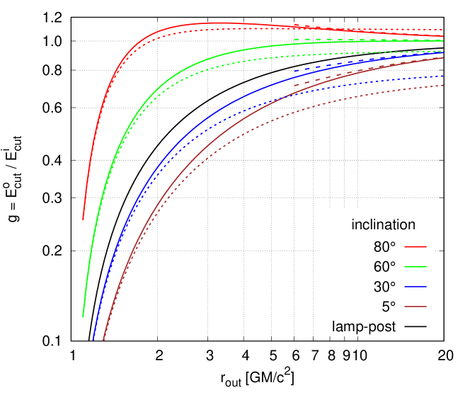
Figure 39: The energy-shift factor plotted as function of an outer radius of a flat disk-like rotating corona, emitting a cutoff-powerlaw ($\Gamma=2$) spectrum, for various inclination angles, assuming constant emissivity for extreme Kerr and Schwarzschild BH (solid and dashed lines, respectively) and a r^-3 emissivity profile for the case of the disk-corona around Kerr BH (dotted lines). The black solid line shows the energy-shift factor in the case of the lamp-post geometry (in this case, the r_out values on x-axis correspond to the height). Adapted from Tamborra et al., [635].

Relativistic effects on the cutoff energy measurements

In previous chapters, we discussed the relation between the spectral high-energy cutoff and the corona temperature. The observationally constrained cut-off energy can thus determine the physical nature of the corona. However, such measurements can be strongly affected by relativistic effects, namely by the gravitational redshift when the corona is compact, or by the Doppler shift when the corona is highly rotating, or by the combination of both.

The relativistic redshift of the high-energy cutoffs was first considered by Fabian et al., [218], who employed the geometry of the corona from the lamp-post height constrained by the reflection models of the soft excess, the iron line, and the Compton hump. The energy shift of the emission from a point on the black-hole rotational axis at a given height $h$ from the centre can be calculated as:

$$g\equiv E_{\rm observed}/E_{\rm intrinsic}=\sqrt{\dfrac{h^{2}-2h+a^{2}}{h^{2}+a^{2}}}.$$ (129)

The observed power-law emission with a high energy cutoff has the form:

$$F_{\rm obs}=NE^{-\Gamma}\exp\left(g\frac{-E}{E^{i}_{cut}}\right).$$ (130)

The lamp-post corona represent, however, a static and dimensionless model. Tamborra et al., [635] considered also the other extreme case – a flat disk co-rotating corona, and noted that a realistic corona should be something in between. In such geometry, the energy shift $g$ is not a single value but is an integrated value over the corona extent. Tamborra et al., [635] showed that the resulting profile of the corona emission can still be approximated by Eq. 130 with a $g$-factor being not a precise value but the fit of the intrinsic integrated emission by a model defined by Eq. 130. Such g-factor is shown in Figure 39 for different considered cases.

The energy shift of the cutoff energy in the disk co-rotating corona model is a function of an outer radius of such corona. If the corona is compact and the outer radius is within a few gravitational radii, then similarly to the lamp-post model, the cutoff energy is more redshifted the more compact the corona is. However, the energy shift in the disk co-rotating corona model strongly depends also on inclination, as it is shown in Figure 39. When compared to the lamp-post model (black solid line in the plot), the larger redshift is obtained for inclinations lower than 30 degrees, and vice versa for higher inclinations. The higher redshift is mainly caused by integration of the corona emission down to the innermost stable circular orbit, but also the transverse Doppler shift contributes to the total redshift in the low-inclined systems. On the other hand, the Doppler boosting of emission coming from the matter moving rapidly towards the observer dominates for highly-inclined systems. As a consequence, the measured cutoff energy may become even blueshifted for inclinations as large as 80 deg.

3 Processes relevant for outflows and jets

“Science progresses best when observations force us to alter our preconceptions."

— Vera Rubin

3.1 Strong-gravity and electromagnetic fields

The electromagnetic field is governed by Maxwell’s equations, the set of first-order differential equations for the electric and magnetic intensity vectors. When expressed in the equivalent (perhaps more elegant) four-dimensional tensorial formalism, the mutually coupled equations can be unified; the electric and the magnetic field components are then comprised in a single quantity. The latter approach is particularly useful in the framework of the Special Theory of Relativity. Whichever of the two equivalent formulations is preferred, one has to tackle differential equations and, therefore, the appropriate initial and boundary conditions must be specified in order to fully determine the structure of the field. As the original literature, review articles and textbooks are numerous on the subject of astrophysical applications of magnetized plasma embedded in combined, mutually interacting gravitational and electromagnetic fields [e.g. 428, 425] we will add to this the context of idealized analytical solutions that allow us to gain some additional insight into physical mechanisms.

The cosmic environment is often ionized and the local electric field component is thus efficiently neutralized in the frame comoving with the highly conducting medium (force-free approximation). On the other hand, magnetic fields are abundant throughout the interstellar and intergalactic space and their intensity can grow to enormous magnitude especially near rotating compact stars and pulsars [264, 65].

Maxwell’s equations are not directly coupled with Newton’s gravitational law; one could thus conclude that there is no immediate relation between the electromagnetic field of the body and its gravitational influence. Not so in General Theory of Relativity. Energy density of the electromagnetic field, as of any other field, stands explicitly in Einstein’s equations for the spacetime structure, contributing as a source of the gravitational field. Einstein’s and Maxwell’s equations must be thus considered simultaneously and this makes the whole system of equations difficult to solve in full generality. Fortunately, the energy density contained in realistic electromagnetic fields turns out to be far too low to influence the spacetime noticeably. Test-field solutions are adequate and accurate enough under such circumstances. Here, by test-field solutions one means the solution of Maxwell’s equations in a fixed (albeit generally curved) spacetime, whose structure can be pre-determined by solving Einstein’s equations with no electromagnetic terms present. Maxwell’s equations are solved afterwards and, by assumption, they have zero impact on the gravitational field. This is also an approximation which we will adopt to start our discussion, but we will abandon it later to see the difference and understand the interaction between Einstein–Maxwell fields.

We first assume the spacetime of a rotating black hole, namely, Kerr metric; see Misner et al., [453]. Different arguments can be put forward to demonstrate that magnetohydrodynamic effects often dominate the behaviour of cosmic plasma and must be taken into account even very close to the black hole event horizon. On the other hand, in the immediate vicinity of the black hole, in particular within the ergosphere of a fast rotating black hole, the gravitational effects must eventually prevail. Also near compact stars the gravitational terms cannot be ignored, and so the general-relativity MHD has to be employed. Here we will confine ourselves to the basic arguments in circumstances where gravitational effects cannot be ignored. The main intention is to describe the assumptions and to suggest selected references that would help entering the complex subject. We will start with axially symmetric and stationary flows, so that the system is further simplified by the presence of the additional symmetries.

The aim of this chapter is to outline the basic equations governing the coupled Einstein–Maxwell field and to mention different limits: the electro-vacuum case vs. MHD case with plasma connected to the evolving magnetic field; and test (weak) electromagnetic fields vs. exact solutions of the full set, where the energy density of the electromagnetic component contributes to the space-time curvature. We will also mention the generating techniques that have been developed in order to find new solutions. These approaches have been found particularly useful in adding the magnetic terms (“magnetizing”) to originally unmagnetized black-holes and to reveal the impact of mutual interaction of Einstein–Maxwell fields. Indeed, this interplay is interesting and non-trivial: asymptotic flatness is lost, singularities develop even outside the event horizon, solutions change their topological classification, etc. We will give references to selected useful works but the limited space does not allow us to present a complete overview; we do not aim to give a comprehensive list of the literature. An extensive pedagogical exposition can be found in textbooks [114, 552, 566].

Let us note that the influence of large-scale magnetic fields upon the space-time metric can be characterized by dimensionless parameter $\beta=B_{0}M$, where $B_{0}$ is the field strength and $M$ is the mass of the object in geometrized units. Considering the above-mentioned limit on the field strength near a one solar-mass compact body, we obtain $\beta\approx 10^{-5}B_{15}(M/M_{\odot})\ll 1$, where $B_{15}=B_{0}/(10^{15}{\rm{G}})$. Such magnetic terms contribute very substantially to the spacetime metric on spatial scales of $r\approx\beta^{-1}$ which in physical units, corresponds to the length-scale of $\approx 10^{5}$ km. In the case of intergalactic fields the magnetic intensity is small, typically below $1\,\mu$G, but near the supermassive black hole the fields frozen into accreting plasma become amplified by many orders. Specifying $M=10^{9}M_{\odot}$ and $B_{0}=10^{4}\,$G we have $\beta=10^{-7}$ and the critical length-scale is $r\simeq 10^{6}R_{\rm g}$. Let us note that the transformation to physical units is achieved by relations $M=GM_{\rm phys}/c^{2}$ for the mass and $B_{0}=G^{1/2}B_{\rm phys}/c^{2}$ for the magnetic field parameter.

Historically, the field of astrophysical MHD has been covered in textbooks and review articles; see, e.g., Cowling, [147]; Melrose, [428]; Zeldovich, [711]; Lynden-Bell, [396]. The applications range from solar physics to accretion disks in galactic nuclei; in our context, the original motivation comes from the studies of particle acceleration near neutron stars where strong electromagnetic fields and inertial effects are present [509, 259, 444], and where the strength of the magnetic intensity is maintained and further enhanced by accretion. Magnetic fields can be amplified by the dynamo action in the disk (Balbus and Hawley, [37]; Krause et al., [363]; Balbus, [36]).

The set of coupled Maxwell’s and Euler’s equations are the essential prerequisites to start with in the classical framework of non-vacuum equations. We can follow a highly simplified exposition with

$${\nabla\times B} = \frac{4\pi}{c}\,\mbox{\boldmath{${j}$}}+\frac{1}{c}\,\frac{\partial\mbox{\boldmath{${D}$}}}{\partial t},\qquad\mbox{\boldmath{${\nabla\cdot B}$}}\;=\;0,$$ (131)

$${\nabla\times E} = -\frac{1}{c}\frac{\partial\mbox{\boldmath{${B}$}}}{\partial t},\qquad\mbox{\boldmath{${\nabla\cdot E}$}}\;=\;4\pi\rho_{\rm e}$$ (132)

with $\rho_{\rm e}$ and ${j}$ being density of all electric charges and currents (e.g., Karas, [318]). Euler’s equation adopts the appropriate form:

$$\rho\,\frac{\partial\mbox{\boldmath$v$}}{\partial t}+\rho\,\mbox{\boldmath$v.\nabla v\;$}=-\mbox{\boldmath$\nabla$}P+\;\mbox{\boldmath$f$}$$ (133)

with

$$\mbox{\boldmath$f$}=\mbox{\boldmath$f$}_{\rm L}+\mbox{\boldmath$f$}_{\rm g}=\rho_{\rm e}\mbox{\boldmath$E$}+c^{-1}\mbox{\boldmath$j\times B$}-\rho\mbox{\boldmath$g$}$$ (134)

being the Lorentz and gravitational terms, respectively. Mainly for the sake of simplification the assumptions about axial symmetry and stationarity are imposed. Although the general relativity effects have not been taken into account, a straightforward reformulation is possible in which the form of the field equations remains almost identical even if strong gravitational fields are present [3+1 formalism; 399, 639].

The primary distinction between the models with and without a black hole consists in different boundary conditions imposed upon the electromagnetic field, which threads the black hole horizon. The relevant Maxwell equations describing the field outside the black hole horizon can be solved by introducing appropriate imaginary currents flowing on the surface of the horizon. These are defined in such a way that the boundary conditions are satisfied. Currents flowing along the field lines can thus close a circuit and the energy extraction is then described in an analogous way as in the discussion of magnetized disks or as in the theory of pulsar emission [82, 113].

Let us first employ the three-vector formalism in the classical form. The above-given equations can be simplified by assuming the force-free approximation,

$$\rho_{\rm e}\mbox{\boldmath$E$}+c^{-1}\mbox{\boldmath$j\times B$}=0.$$ (135)

The physical interpretation and consequences of the above relation require a thorough discussion. Equation (135) tells us that inertia of the material is neglected. In other words, the influence of the Lorentz force acting on plasma in the comoving frame gets neutralized immediately by induced electric currents; perfect conductivity is thus assumed. A dimension-less condition for the validity of the force-free approximation is $\rho\Gamma v^{2}/B^{2}\ll 1$. This corresponds to a similar assumption of ideal MHD,

$$\mbox{\boldmath$E^{\prime}\;$}\equiv\,\mbox{\boldmath$E\;$}+\,c^{-1}\,\mbox{\boldmath$v\times B\;$}=0;$$ (136)

where $E^{\prime}\;$ is the electric field in the local system attached to plasma, and the two forms become equivalent if the current density is proportional to the velocity of the medium, $\mbox{\boldmath{${j}$}}=\rho_{\rm e}\mbox{\boldmath{${v}$}}$. A more general formula for the current density that still satisfies the force-free assumption (135) has a form $\mbox{\boldmath{${j}$}}=\rho_{\rm{}e}\mbox{\boldmath{${v}$}}+\mu\mbox{\boldmath{${B}$}};$ $\mu$ is a scalar function to be determined. Both the force-free and the perfect MHD fields are degenerate, i.e. $E\cdot B\;$$=0$. The approximation of ideal MHD can be understood as an assumption about perfect electric conductivity of the material. Substituting

$$\mbox{\boldmath{${j}$}}=\sigma\mbox{\boldmath{${E}$}}^{\prime}$$ (137)

for the vector of electric field from Ohm’s law ($\sigma$ designates specific conductivity of the medium) and assuming perfect conductivity $(\sigma\rightarrow\infty)$, we find

$$\mbox{\boldmath$\nabla\times\,$}(\mbox{\boldmath$v\times B$})=\frac{\partial\mbox{\boldmath$B$}}{\partial t}.$$ (138)

Equation (138) expresses the freezing of the magnetic field in plasma material. The reason for this denomination is evident upon realizing that the magnetic flux across an imaginary loop ${\ell}$ flowing together with the medium can be written as a sum of two terms, the first one being determined by motion of the loop,

$$\int_{\cal S}\mbox{\boldmath$\nabla\times\,$}(\mbox{\boldmath$v\times B$})\mbox{\boldmath$\cdot$}d\mbox{\boldmath$\cal S$}=\oint_{\ell}(\mbox{\boldmath$v\times B$})\,\mbox{\boldmath$\cdot$}d\mbox{\boldmath$\ell$}=-\oint_{\ell}\mbox{\boldmath$B\cdot$}(\mbox{\boldmath$v\times$}d\mbox{\boldmath$\ell$}).$$ (139)

The term $\partial$$B$$/\partial t$ on the right-hand side of (138) corresponds to the change of the magnetic flux due to the explicit time-dependence of $B$,

$$\int_{\cal S}\frac{\partial\mbox{\boldmath$B$}}{\partial t}\,\mbox{\boldmath$\cdot\,$}d\mbox{\boldmath$S$}.$$ (140)

Equation (138) thus expresses the fact that the magnetic flux across any arbitrary closed loop remains constant. As we have seen before, one can also understand this equation as a condition for the electric field to vanish in the rest frame of plasma.

Now we can examine the basic relations valid of axially symmetric magnetohydrodynamic equilibrium configurations under forces of (weak) gravity. The relevant equations are capable of describing, for example, magnetospheres and collimated outflows from aligned rotators and magnetized accretion disks, as derived in detail by Camenzind, [113] and Lovelace et al., [392]. To remind the reader about the assumption, we adopt the axial symmetry and stationarity: we set $\partial/\partial\phi=0$, $\partial/\partial{t}=0$ in all formulae. Starting equations are the mass conservation law (the continuity equation); the momentum conservation law (Euler equation, supplemented by the relation for the external force $\mbox{\boldmath{${f}$}}=\frac{1}{c}\,\mbox{\boldmath{${j\times B}$}}-\rho\mbox{\boldmath{${g}$}}$, where we assume an electrically neutral plasma, $\rho_{\rm e}=0)$; and Maxwell’s equations with the perfect MHD constraint. The gravitational acceleration ${g}$ is linked to density via the Poisson equation, $\nabla^{2}\Phi=4\pi G\rho$, and, finally, it has to be supplemented by the first law of thermodynamics and the equation of state to close the set of equations.

It follows from Faraday’s law together with the conditions of axial symmetry and stationarity ($\mbox{\boldmath{${\nabla\times E}$}}=0$) that the toroidal part $\mbox{\boldmath{${E}$}}_{\rm T}$ of electric field vanishes,

$$E_{\phi}^{2}=\mbox{\boldmath{${E}$}}_{\rm T}\mbox{\boldmath{${\cdot E}$}}_{\rm T}=0.$$ (141)

The condition of perfect MHD implies the relation for the poloidal flow velocity

$$\mbox{\boldmath{${v}$}}_{\rm P}=\xi\mbox{\boldmath{${B}$}}_{\rm P},$$ (142)

where $\xi(R,z)$ is a (yet undetermined) scalar function. It is advantageous at this point to introduce into the Maxwell equations the vector potential ${A}$ and the scalar magnetic flux function, $\Psi(R,z)\equiv RA_{\phi}$. Components of $\mbox{\boldmath{${B}$}}_{\rm P}$ in terms of $\Psi$ read $B_{R}=-\Psi_{,z}/R$, $B_{z}=\Psi_{,R}/R,$ where the coma denotes partial differentiation. It is now evident from equation (142) that

$$4\pi\rho\xi=F_{1}(\Psi),$$ (143)

where $F_{1}(\Psi)$ is an arbitrary function to be specified by the boundary conditions and symmetries of the required solution. (We have applied the Maxwell equation $\mbox{\boldmath{${\nabla\cdot B}$}}=\mbox{\boldmath{${\nabla\cdot B}$}}_{\rm P}=0,$ and the continuity equation.) We will see that there is a set of such functions of $\Psi$ that determine a specific solution. Each function can be identified with some conserved quantity (derivation of $F_{1}$ utilizes the mass conservation equation). The existence of flux functions, which remain constant on magnetic surfaces $\Psi={\rm const}$, is crucial in investigating axisymmetric hydromagnetic flows (see Chandrasekhar, [124]).

It follows from $\mbox{\boldmath{${v}$}}_{\rm P}=\xi\mbox{\boldmath{${B}$}}_{\rm P}$ [Eq. (142)] that

$$\mbox{\boldmath{${v\times B}$}}=\mbox{\boldmath{${v_{\rm T}\times B_{\rm P}}$}}+\mbox{\boldmath{${v_{\rm P}\times B_{\rm T}}$}}=\frac{v_{\phi}-\xi B_{\phi}}{R}\,\mbox{\boldmath{${\nabla}$}}\Psi.$$ (144)

Curl of the last equation vanishes in accordance with the perfect MHD condition and Faraday’s law so that another stream function, $F_{2},$ can be introduced in the following way:

$$\frac{v_{\phi}-\xi B_{\phi}}{R}=F_{2}(\Psi),\qquad\mbox{\boldmath{${E}$}}=-c^{-1}F_{2}(\Psi)\mbox{\boldmath{${\nabla}$}}\Psi.$$ (145)

Further relations are obtained by projections of the Euler equation and can be derived via straightforward but lengthy manipulations. The toroidal part reads

$$\mbox{\boldmath{${B}$}}_{\rm P}\mbox{\boldmath{${\cdot\nabla}$}}\left(RB_{\phi}-F_{1}Rv_{\phi}\right).$$ (146)

For analogous reasons as those that have been presented with equation (142), the term in parentheses is also a function of $\Psi$ only, say $F_{3}(\Psi)$. Other two independent relations can be obtained by projecting the Euler equation into the poloidal plane. The projection along $\mbox{\boldmath{${B}$}}_{\rm P}$ yields the Bernoulli equation

$${\textstyle{\frac{1}{2}}}\,v^{2}+\int_{\Psi={\rm const}}\frac{{\rm d}P}{\rho}+\Phi-Rv_{\phi}F_{3}=F_{4}(\Psi).$$ (147)

Compared to the hydrodynamical form of the Bernoulli integral, in which electromagnetic effects are not considered, the additional term $Rv_{\phi}F_{3}$ corresponds to the electromagnetic (Poynting) energy transport. The projection of the poloidal component of the Euler equation to the direction parallel to $\mbox{\boldmath{${\nabla}$}}\Psi$ serves as a Grad–Shafranov master equation that can close the set of independent equations (for the application to black hole magnetospheres, see e.g. Blandford and Znajek, [85]; Beskin and Kuznetsova, [66]; Ioka and Sasaki, [307]; Contopoulos et al., [143]). This is a non-linear differential equation for $\Psi,$ the explicit form of which naturally depends on the equation of state and on stream functions $F_{k}$. For example, we set $F_{1}=0$ if no poloidal flow of material is required a priori (the case of disks). Force-free approximation to the Grad–Shafranov equation is equivalent to the self-consistent form of the pulsar equation from the astrophysical literature (Cohen et al., [136], Scharlemann and Wagoner, [580]). Within the general relativity framework, its applications to rotating compact stars and black holes have been examined by various authors (see e.g. Kim et al., [344]). On the other hand, laboratory plasma in tokamaks are often described within the approximation of a vanishing material flow, $F_{1}=F_{2}=0,$ and negligible gravity, $\Phi=0$.

Electromagnetic forces act on charged particles and may substantially modify the structure of accretion disks. These have been originally explored in a series of papers by Michel, [444], Michel, [445]. The inclusion of electromagnetic effects makes the disk theory much more complex. A simplified approach is possible in terms of self-similar solution of axially symmetric MHD equations [355].

Let us consider a magnetized accretion disk in the equatorial plane and assume that the magnetic field is frozen into the disk. The toroidal part of the field arises from the dragging of the magnetic field by the disk material. It follows that $\mbox{\boldmath{${B}$}}_{\rm T}=B_{\phi}\,\mbox{\boldmath{${e_{\phi}}$}},$ $\mbox{\boldmath{${B}$}}_{\rm P}=\mbox{\boldmath{${B}$}}-\mbox{\boldmath{${B}$}}_{\rm T}=B_{R}\,\mbox{\boldmath{${e_{R}}$}}+B_{z}\,\mbox{\boldmath{${e_{z}}$}}$.

Now the basic relations adopt the following form. The Maxwell equation $\mbox{\boldmath{${\nabla\cdot B}$}}=0$ together with the consequence of axial symmetry, $\mbox{\boldmath{${\nabla\cdot B_{\rm T}}$}}=0,$ yield $\mbox{\boldmath$\nabla\cdot B_{\rm P}$}=0$. This means that both the poloidal and the toroidal components can be separately associated with unending field lines. The value of $E_{\rm P}$ follows from the force-free condition,

$$0=\mbox{\boldmath{${E}$}}^{\prime}=\mbox{\boldmath{${E}$}}_{\rm P}+c^{-1}(\mbox{\boldmath{${\Omega\times r}$}})\mbox{\boldmath{${\times B}$}},$$ (148)

where $\mbox{\boldmath{${\Omega}$}}=\Omega^{\rm F}\,\mbox{\boldmath{${e_{\phi}}$}}$ means the angular velocity of each field line and $r$ is the radius vector. Charged particles move along field lines. Using $\mbox{\boldmath{${\nabla\times E_{\rm P}}$}}=0$ and $\mbox{\boldmath{${\nabla\cdot B_{\rm P}}$}}=0$ we find

$$\mbox{\boldmath{${B_{\rm P}\cdot\nabla}$}}\Omega^{\rm F}=0.$$ (149)

In other words, the angular velocity of each field line remains constant along its curve; thus $\Omega^{\rm F}$ does not change along poloidal field lines. This result is called Ferraro’s law of iso-rotation [232].

The light surface is the locus of points where the velocity of the field lines approaches the speed of light. Charged particles cannot corotate with field lines beyond the light surface; instead, they are forced to move away and this is the basis of particle acceleration around pulsars and possibly formation of jets in extragalactic sources. On the other hand, the accretion disk itself can serve as a source of particles. Assuming the perfect MHD condition inside the disk, we obtain for the particle density

$$n=\frac{1}{4\pi q_{\rm e}}\mbox{\boldmath$\nabla\cdot E$}\;=-\frac{1}{4\pi q_{\rm e}c}\;\mbox{\boldmath$\nabla\cdot$}(\mbox{\boldmath$v\times B$})=-\frac{1}{2c}\Omega B_{\phi}.$$ (150)

Non-zero charge-density generates an electric field, which pulls charged particles out of the disk.

Magnetic field lines threading the disk exert a torque on its material, $\mbox{\boldmath{${G}$}}=\mbox{\boldmath{${R\,\times}$}}\,(\mbox{\boldmath{${j\times B}$}})$, and are thus a source of effective viscosity. Such a disk does not radiate (remember that we are considering axisymmetric stationary configurations). Consider now a circle of radius $R$ centered on the symmetry axis. Ampere’s law yields $B_{\rm T}={2J}/{cR}$. We have already mentioned that in the force-free region currents flow along magnetic surfaces, but in the disk and in the far region the force-free condition is violated and dissipation occurs. The density of the electromagnetic energy flowing through the force-free region is given by $\mbox{\boldmath{${P}$}}=c\,\mbox{\boldmath{${E\times B}$}}\approx c\,\mbox{\boldmath{${E_{\rm P}\times B_{\rm T}}$}}$. Substituting for $E_{\rm P}$ from Eq. (148) we estimate the magnitude of this vector as ${\cal P}\approx\Omega RB_{\rm P}B_{\rm T}$. Finally, $B_{\rm P}$ and $B_{\rm T}$ are to be determined in accordance with the boundary conditions.

Magnetohydrodynamic equations are only applicable if the medium can be treated as a continuum. This assumption does not hold in case of highly diluted, in which case the mean free path of particles is comparable with other characteristic length-scales of the system; small-scale turbulence may save the MHD approximation even at low densities but large-scale magnetic fields break it in regions of strong magnetic dominance [311]. There are various possibilities for extending the validity of the description in terms of continuum beyond the ideal limit towards to include effects of finite resistivity. For example, unequal directional action of the magnetic field on charged particles can be accommodated by replacing the scalar conductivity $\sigma$ in Ohm’s law by a tensorial quantity. Eventually, the extreme situations of highly rarefied magnetized plasma can be adequately described only by adopting the kinetic theory.

In the guiding-center approximation one assumes that local gyrations and slow-drift motions can be neglected [380]. This restriction requires the radius of the gyrations be much less than a characteristic length-scale of the field inhomogeneities, and the period of the gyrations to be much less than a characteristic time-scale of the field evolution. If the conditions are satisfied one can average out gyrations and drifts. Instead of the exact trajectory, one follows an imagined path of the center of gyrations. Flow lines of plasma coincide with the common direction of electric and magnetic fields in the plasma co-moving frame. The equation of motion of a particle of rest mass $m_{0}$ and electric charge $q$ then reads [332]

$$\frac{d}{dt}\left(\Gamma m_{0}\mbox{\boldmath{${v}$}}\right)=\Gamma m_{0}\mbox{\boldmath{${g}$}}+\frac{q}{c}\,(\mbox{\boldmath{${E}$}}+\frac{1}{c}\mbox{\boldmath{${v\times B}$}}),$$ (151)

where $\Gamma$ is the Lorentz factor and ${g}$ is the gravitational acceleration.

3.2 General Relativity framework

Let us now generalize our discussion to the case of General Relativity (GR) framework for axially symmetric MHD flows. In this section, very naturally, we will employ the standard GR notation with geometrized units ($c=G=1$) and the signature of metric $-\mbox{+++}$. First we will still maintain the approximation of electromagnetic test fields (albeit in the curved background), so that the spacetime metric is not electromagnetically influenced. The set of equations of perfect magnetohydrodynamics can be written in the following form [22, 385].

Let us note that the environment of diluted cosmic plasma, accretion flows in particular, has been permeated by magnetic fields of diverse magnitude and topology. In the context of black-hole accretion the field lines can be either turbulent and highly entangled (on length-scales $\ell\ll R_{\rm g}$, or they can be organized on much larger scales, as various simulations indicate in the evacuated regions along the symmetry axis. Also time-scales vary wildly, from the fields that change explosively (compared to the light-crossing time across the event horizon, $\tau_{\ell}\simeq\ell/c$) to steady systems that evolve adiabatically over much longer (viscous) period. In following, to reveal effects connected with the overall geometry of the system and associated effect of gravitation, we will concentrated on large-scale, organized, slowly evolving fields.

Conservation of the particle number reads $\left(\rho_{0}u^{\alpha}\right)_{;\alpha}=0$, with $\rho_{0}=mn;$, where $m$ is the particle rest mass, $n$ numerical density, $u^{\alpha}$ four-velocity. Here we do not consider a possibility of creation of pairs, which would break this conservation law. Normalization condition for four-velocity is written $u^{\alpha}u_{\alpha}=-1$. As originally shown by Znajek, [719], by employing the explicit form of the energy-momentum conservation ${T^{\alpha\beta}}_{;\beta}=0$, and the definition of energy-momentum tensor in terms of material density $\rho$ and pressure $P$, one finds [537]

$$T^{\alpha\beta}=T^{\alpha\beta}_{\rm matter}+T^{\alpha\beta}_{\rm EMG},$$ (152)

where the right-hand side contains the source term divided in two components,

$$T^{\alpha\beta}_{\rm matter} = (\rho+p)u^{\alpha}u^{\beta}+pg^{\alpha\beta},$$ (153)

$$T^{\alpha\beta}_{\rm EMG} = \frac{1}{4\pi}\left(F^{\alpha\mu}F^{\beta}_{\mu}-\frac{1}{4}F^{\mu\nu}F_{\mu\nu}g^{\alpha\beta}\right),$$ (154)

with $F_{\mu\nu}=A_{\nu,\mu}-A_{\mu,\nu}$.

The axial symmetry and stationarity guarantee the existence of two Killing vectors, $k^{\alpha}=\delta^{\alpha}_{t}$ and $m^{\alpha}=\delta^{\alpha}_{\phi}$, which satisfy relations

$$0=k_{\alpha}{T^{\alpha\beta}}_{;\beta}=\left(k_{\alpha}T^{\alpha\beta}\right)_{;\beta},$$ (155)

$$0=m_{\alpha}{T^{\alpha\beta}}_{;\beta}=\left(m_{\alpha}T^{\alpha\beta}\right)_{;\beta}.$$ (156)

Let us note that the electromagnetic field may or may not conform to the same symmetries as the gravitational field. Naturally, the problem is greatly simplified by assuming axial symmetry and stationarity for both fields.

In the fluid rest frame, the electric field is assumed to vanish completely: $F_{\alpha\beta}u^{\beta}=0$. It follows [719, 85, 292, 343, 516]

$$\frac{A_{t,r}}{A_{\phi,r}}=\frac{A_{t,\theta}}{A_{\phi,\theta}}\equiv-\Omega^{\rm F}.$$ (157)

The latter relation implies ${\Omega^{\rm F}_{,r}}/{\Omega^{\rm F}_{,\theta}}={A_{\phi,r}}/{A_{\phi,\theta}}$. Indeed, Eq. (157) is an analogy of Eq. (148) with $\Omega^{\rm F}$ playing the role of angular velocity of magnetic field lines. A more detailed exposition and derivation of these relations can be found in Phinney, [537], where it is shown that the latter equation implies that the two Jacobian matrices

$$\frac{\partial(A_{t},A_{\phi})}{\partial(r,\theta)}=0,\qquad\qquad\frac{\partial(\Omega^{\rm F},A_{\phi})}{\partial(r,\theta)}=0$$ (158)

vanish. Therefore, the mentioned functions are not independent: $A_{t}\equiv A_{t}(A_{\phi})$ and $\Omega^{\rm F}\equiv\Omega^{\rm F}(A_{\phi})$. The flow stream-lines and the magnetic field-lines lie in the level surfaces of $A_{\phi},$ i.e. $\vec{u}\cdot\nabla A_{\phi}=\vec{B}\cdot\nabla A_{\phi}=0,$ where $\vec{B}=(^{*}{F})\cdot\vec{u}$ (the arrow denotes two-component space-like vectors defined in the $(r,\theta)$-plane).

In order to find the possible geometry of flow lines, one can introduce the stream function $k(r,\theta)$ satisfying [537, 491]

$$\frac{u^{r}}{A_{\phi,\theta}}=-\frac{u^{\theta}}{A_{\phi,r}}\equiv\frac{k(r,\theta)}{4\pi\sqrt{-g}\rho_{0}};$$ (159)

apparently, the functional dependence is constrained to $k(r,\theta)\equiv k(A_{\phi})$. Two additional stream functions can be obtained by inserting the explicit form of $T^{\alpha\beta}$ into equations (155)–(156). Finally, we are still left with the two equations, ${T^{r\beta}}_{;\beta}=0$ and ${T^{\theta\beta}}_{;\beta}=0,$ but also these relations are not independent and they can be constrained by contracting ${T^{\alpha\beta}}_{;\beta}=0$ with any poloidal four-vector which is linearly independent of poloidal projection of $u_{\alpha}$. The result is a non-linear second-order differential equation which is a generalization of the Grad–Shafranov equation within general relativity [as outlined by 344].

So far our discussion has been restricted to weak, electromagnetic test-fields in a given, fixed background spacetime; we have neglected the influence of the electromagnetic field on the spacetime metric. This approach was employed by a number of authors to address the problem of electromagnetic effects near a rotating (Kerr) black hole [639, 664, 634, 354]. The Kerr solution is a suitable and astrophysically accurate approximation of the space-time that captures cosmic environment relevant for the formation of jets [229]. On the other hand, self-consistent solutions of coupled Einstein–Maxwell equations for black holes immersed in electromagnetic fields have been studied only within stationary, axially symmetric, vacuum models [e.g., 242, 179, 241, 215, 293, 332].

It turns out that the test electromagnetic field approximation is fully adequate for modelling astrophysical sources, however, the long-term evolution of magnetospheres of rotating black holes, consequences of non-ideal MHD and the effects of oscillatory motion of the central body are still open to further work [499, 521, 565, 564, 368].

Electromagnetic fields play an important role in astrophysics. Near rotating compact bodies, such as neutron stars and black holes, the field lines are deformed by an interplay of rapidly moving plasma and strong gravitational fields. Here we will illustrate purely gravitational effects by exploring simplified vacuum solutions in which the influence of plasma is ignored but the presence of strong gravity is taken into account. In fact, we will restrict ourselves to purely electro-vacuum solutions for which we we will outline the elegant formalism of null tetrads. We do not derive new solutions or technique in these lectures, instead, we summarise useful relations with the focus towards the role of large-scale organised fields interacting with rotating black holes.

Let us note that, with exact solutions of the coupled Einstein–Maxwell electro-vacuum fields, an aligned magnetic flux becomes expelled from a rotating black hole as an interplay between the shape of magnetic lines of force (which become pushed out of the horizon) and the concentration of the magnetic flux tube toward the rotation axis (which becomes more concentrated for strong magnetic fields because of their own gravitational effect). This is, however, important only for very strong magnetic fields. In the the latter case the classical definition of the black hole [285] has to be modified by taking into account the fact the spacetime is not asymptotically flat; instead, the electromagnetic effects contribute to the gravitational field and they may even produce singularities outside the event horizon (see Ernst and Wild, [215]; Karas and Vokrouhlický, [332], and further references cited therein).

Now we are in a position to discuss weak test electromagnetic fields near black holes, which will then lead us to the methods to generate exact stationary (axially symmetric) solutions. We start with Einstein’s equations in the form of a set of coupled partial differential equations [e.g., 125],

$$R_{\mu\nu}-\textstyle{\frac{1}{2}}Rg_{\mu\nu}=8\pi T_{\mu\nu}$$ (160)

($c=G=1$), where the right-hand side (the source term $T_{\mu\nu}$) is assumed to be of purely electromagnetic origin,

$$T^{\alpha\beta}\equiv T^{\alpha\beta}_{\rm EMG}=\frac{1}{4\pi}\left(F^{\alpha\mu}F^{\beta}_{\mu}-\frac{1}{4}F^{\mu\nu}F_{\mu\nu}g^{\alpha\beta}\right).$$ (161)

The sources are constrained by the conservation relation, ${T^{\mu\nu}}_{;\nu}=-F^{\mu\alpha}j_{\alpha}$, where ${F^{\mu\nu}}_{;\nu}=4\pi j^{\mu}$, ${{}^{\star}F^{\mu\nu}}_{;\nu}=4\pi\mathcal{M}^{\mu}$, and the dual tensor is denoted by ${}^{\star}F_{\mu\nu}\equiv\frac{1}{2}{\varepsilon_{\mu\nu}}^{\rho\sigma}F_{\rho\sigma}$.

We assume that the electromagnetic test-fields reside in a curved background of a rotating black hole (Kerr metric; see Thorne et al., [639]; Gal’tsov, [241]). In other words, we study magnetised spacetimes that possess a horizon within classical General Relativity. Let us note that higher-dimensional black holes and black rings in external magnetic fields have attracted a lot of interest in recent years and they have been explored by, e.g., Ortaggio, [501] and Yazadjiev, [691]. Also an extension to the case of naked singularity has been discussed recently [8].

The presence of Killing vectors corresponds to symmetries of the spacetime [125, 668], namely, stationarity and axial symmetry. Killing vectors satisfy the relation

$$\xi_{\mu;\nu}+\xi_{\nu;\mu}=0,$$ (162)

where the coordinate system can be selected in such a way that the symmetry generating vector adopts a simple form with the only non-vanishing component: $\xi^{\mu}=\delta^{\mu}_{\rho}$. In a vacuum spacetime, Killing vectors generate a test-field solution of Maxwell equations. One can check that a sequence of relations is obeyed:

$$0=\xi_{\mu;\nu}+\xi_{\nu;\mu}=\xi_{\mu,\nu}-\Gamma^{\lambda}_{\mu\nu}\xi_{\lambda}+\xi_{\nu,\mu}-\Gamma^{\lambda}_{\mu\nu}\xi_{\lambda}=g_{\mu\nu,\rho}.$$ (163)

Eq. (163) states that the metric tensor, due to the symmetry, is independent of the selected $x^{\rho}$ coordinate. In fact, the electromagnetic field may or may not conform to the same symmetries as the gravitational field. Naturally, the problem is greatly simplified by assuming axial symmetry and stationarity for both fields.

We define the electromagnetic field by associating it with the Killing vector field, $F_{\mu\nu}=2\xi_{\mu;\nu}$. Then it turns out that $F_{\mu\nu}=2\xi_{\mu;\nu}=-2\xi_{\nu;\mu}=-F_{\nu\mu}$, and hence the symmetry vector generates the electromagnetic test field tensor in the form [668]

$$F_{\mu\nu}=\xi_{\mu;\nu}-\xi_{\nu;\mu}\equiv\xi_{[\mu;\nu]}.$$ (164)

By employing the Killing equation and the definition of Riemann tensor, i.e., the relations $\xi_{\mu;\nu;\sigma}-\xi_{\mu;\sigma;\nu}=-R_{\lambda\mu\nu\sigma}\xi^{\lambda}$, and $R_{\lambda[\mu\nu\sigma]\mathrm{cycl}}=0$, we find

$$\xi_{\mu;\nu;\sigma}=R_{\lambda\sigma\mu\nu}\xi^{\lambda},\qquad{\xi^{\mu;\nu}}_{;\nu}={R^{\mu}}_{\lambda}\xi^{\lambda}.$$ (165)

The right-hand side vanishes in vacuum, hence ${F^{\mu\nu}}_{;\nu}=0$. It follows that the well-known field invariants are given by relations

$$\mbox{\boldmath$E.B$}=\textstyle{\frac{1}{4}}\,{{}^{\star}}F_{\mu\nu}F^{\mu\nu},\qquad B^{2}-E^{2}=\textstyle{\frac{1}{2}}F_{\mu\nu}F^{\mu\nu}.$$ (166)

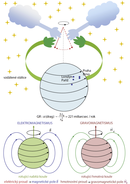
Figure 40: Artist’s conception of the Mach’s principle and its link to the frame-dragging in General Relativity. A heuristic approach pictures the averaged motions of matter in the Universe as the basis of local inertial systems. Particles as well as fields “feel” gravitational effect by matter in rotation. This is the Lense–Thirring effect that influences the motion of Foucault pendulums, which is shown at the top of the plot. In the bottom part, according to the General Relativity, in analogy with the electromagnetic field of a rotating charged sphere, a rotating body creates the gravitomagnetic field in its surroundings [43, 514]. The analogy demonstrates an inspiring role that the Mach’s principle plays in gravitational physics, even if it is only partially incorporated in GR. This drawing has been adopted from the Czech review article (J. Bičák [78]) dedicated to the centenary anniversary of Ernst Mach’s death (*1838 $\dagger$1916); figure by Jana Musilová was presented by Jiří Bičák during “Mach, Relativity and Cosmology” conference in Brno (2016). The original drawing with a Czech legend indicates distant stars (yellow), a rotating charged sphere in electromagnetism (green), and a rotating massive sphere according to gravitomagnetism (red).

We start from the axial and temporal Killing vectors, existence of which is guaranteed in any axially symmetric and stationary spacetime,

$$\xi^{\mu}=\frac{\partial}{\partial t},\qquad\tilde{\xi}^{\mu}=\frac{\partial}{\partial\phi}.$$ (167)

In the language of differential forms (e.g. Wald, [668]),

$$\underbrace{\textstyle{\frac{1}{2}}F_{\mu\nu}{\,\rm d}x^{\mu}\wedge{\,\rm d}x^{\nu}}_{\mbox{${\bf F}$}}=\underbrace{\xi_{\mu,\nu}{\,\rm d}x^{\mu}\wedge{\,\rm d}x^{\nu}}_{\mbox{${\bf d}${\boldmath$\xi$}}}.$$ (168)

The above-given equations allow us to introduce the magnetic and electric charges in the form of integrals over the horizon. Magnetic charge is defined by relation

$$4\pi\mathcal{M}=\int_{\mathcal{S}}{\bf F}=\int_{\mathcal{S}}\mbox{${\bf d}${\boldmath$\xi$}},$$ (169)

which is identical to zero as expected, while the electric charge is defined

$$4\pi Q=\int_{\mathcal{S}}\mbox{\boldmath${}^{\star}F$}=\int_{\mathcal{S}}\mbox{{\boldmath${}^{\star}$}${\bf d}${\boldmath$\xi$}},$$ (170)

which evaluates to $Q=-2M=4J$, where $M$ has a meaning of mass and $J$ is angular momentum of the source. Here, integration is supposed to be carried out far from the source, i.e. in spatial infinity of Kerr metric in our case.

In an asymptotically flat spacetime, $\partial_{\phi}$ generates a uniform magnetic field, whereas the field vanishes asymptotically for $\partial_{t}$. These two solutions are known as the Wald’s field [667, 347, 69, 476],

$$F=\textstyle{\frac{1}{2}}B_{0}\left({\,\rm d}\tilde{\xi}+\frac{2J}{M}{\,\rm d}\xi\right).$$ (171)

Magnetic flux surfaces are given by integration, $4\pi\Phi_{\mathcal{M}}=\int_{\mathcal{S}}\mbox{\boldmath$F$}=\mbox{const}$. Magnetic field lines in the axisymmetric case are then

$$\frac{{{\,\rm d}{r}}}{{{\,\rm d}\theta}}=\frac{B_{r}}{B_{\theta}}.$$ (172)

This definition is in agreement with the natural expectation that the magnetic lines should reside in the surfaces of constant magnetic flux.

This brings us to the spin-coefficient formalism [487, 250] as a special form of the tetrad formalism. Although this should be a topic of an independent text beyond the scope of the present chapter, we refer the reader to Appendix 5.1 for an introduction and the basic notation related to the highly useful method of spin coefficients.

An explicit form of the solutions can be constructed and illustrated by plotting the lines of force where the Schwarzschild case is among the simplest examples, where the effects of strong gravitational field persist [320, for further references].

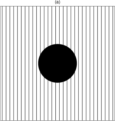
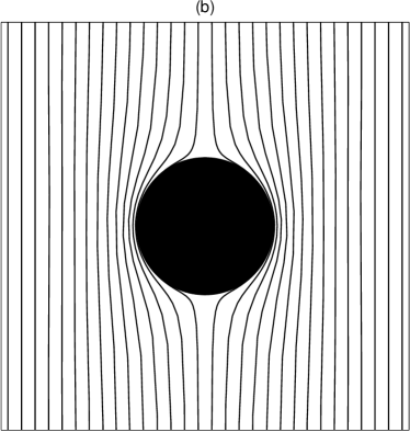
Figure 41: The poloidal ($\phi=$ const) section across a system of the black hole (black circle) embedded in an axially symmetric (weak) uniform magnetic field: (a) $a=0$ (static black hole – Schwarzschild solution for the space-time geometry) vs. (b) $a=M$ (maximally rotating Kerr black hole). In the left panel (a), magnetic lines of force are plotted for the non-rotating case in Schwarzschild coordinates, where the gravitational effects on the homogeneous field lines do not show up in the projection. On the other hand, the right panel (b) does show the effect of the expulsion due to fast rotation that influences the spacetime and the magnetic field.

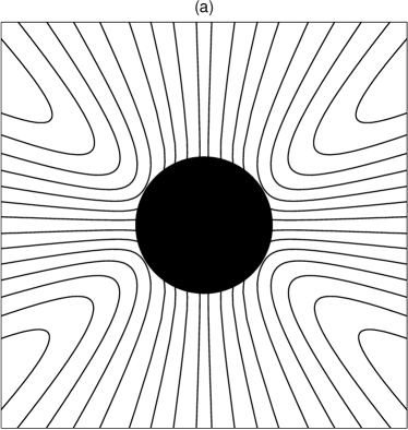
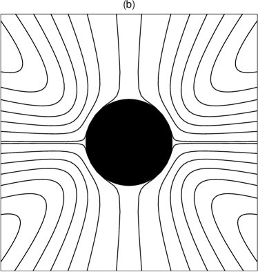
Figure 42: Field lines of the gravito-magnetically induced electric field produced by the aligned, asymptotically uniform (test) magnetic field in vacuum. (a) The case of a fast-rotating Kerr black hole ($a=0.95M$); (b) the maximally rotating black hole ($a=M$). Let us notice the specific form of the induced electric field which becomes radial at the larger distance. Figure adapted from Dovčiak et al., [186].

Lorentz force acts on electric/magnetic monopoles residing at rest with respect to a locally non-rotating frame (fig. 40),

$$\frac{{\,\rm d}u^{\mu}}{{\,\rm d}\tau}\propto\,^{\star}\!F^{\mu}_{\nu}\,u^{\nu},\qquad\frac{{\,\rm d}u^{\mu}}{{\,\rm d}\tau}\propto F^{\mu}_{\nu}\,u^{\nu}.$$ (173)

Magnetic lines are defined in the form [130]

$$\frac{{\,\rm d}r}{{\,\rm d}\theta}=-\frac{F_{\theta\phi}}{F_{r\phi}},\qquad\frac{{\,\rm d}r}{{\,\rm d}\phi}=\frac{F_{\theta\phi}}{F_{r\theta}},$$ (174)

whereas the magnetic flux (in an axially symmetric case) reads

$$\Phi_{\rm m}=\pi B_{0}\left[r^{2}-2Mr+a^{2}+\frac{2Mr}{r^{2}+a^{2}\,\cos^{2}\!\theta}\left(r^{2}-a^{2}\right)\right]\sin^{2}\!\theta=\mbox{const}.$$ (175)

The shape of field lines in the poloidal projection is associated with the coordinates, whereas the magnetic flux is an invariantly defined scalar quantity that characterizes the system. Notice: $\Phi_{\rm m}=0$ for $r=r_{+}$ and $a\rightarrow M$. The axisymmetric flux is expelled out of the horizon – a somewhat surprising but well-known effect that resembles the Meissner effect in physics of (super-)conducting magnetized bodies [72, 529, 71]. The analogy, however, is not complete. While the true Meissner effects concerns the magnetic field expulsion out of superconducting medium, its black-hole variant describes a strong gravity influence on the field lines in vacuum spacetime with a specific high degree of symmetry.

Let us note that the mechanism operates not only in case of asymptotically uniform magnetic fields but it similarly influences higher multipoles. Apparently, the effect does not operate in oblique (non-axisymmetric) or plasma filled (force-free) or non-stationary magnetospheres [515, 260, 189]. There has been a continued discussion whether the process of expulsion might operate in the case of Kerr black hole in extreme rotation ($a/M=\pm 1$); it turns out, however, that the mechanism is relevant just for electro-vacuum fields and non-ideal MHD environments. In particular, the force-free condition (typically satisfied in highly conducting cosmic environments) leads to magnetic field lines being rapidly accreted together with the infalling matter, so that the magnetic flux tubes penetrate the horizon in an almost radial direction.

On the other hand, we will demonstrate further below that the electro-vacuum case is not limited to weak magnetic fields; it can be reproduced within the exact electro-vacuum axisymmetric solutions of the coupled Einstein–Maxwell equations if the notion of the black hole is appropriately extended. This is in agreement with the view of the GR Meissner effect as a purely geometrical effect that influences the vacuum structure of the magnetic field lines around the event horizons, however, it neither enhances nor counter-acts the competition from MHD processes when a conducting (non-vacuum) environment is present.

The electric fluxes and field lines can be introduced in an analogous manner by interchanging the electromagnetic field tensor and its dual tensor, and simultaneously the magnetic charge by the electric charge, and vice versa wherever they appear in the formulae. The induced electric field vanishes in the non-rotating case. Based on analogy with a conducting sphere in rotation (within the classical electromagnetism), one could expect a quadrupole-type component, however, here the leading term of the electric field arises due to gravo-magnetic interaction, which is a purely general-relativity effect. This electric field falls off radially as $\propto r^{-2}$ (Fig. 42).

Magnetic field lines reside in surfaces of constant magnetic flux, and this way the lines of force are defined in an invariant way (see Fig. 41). An electric field is induced by the gravito-magnetic influence of the black hole. The resulting field lines are shown in Fig. 42. An asymptotic form of the electric field-lines reads

$$\frac{{\,\rm d}r}{{\,\rm d}\lambda} = \frac{B_{0}aM}{r^{2}}\left(3\cos^{2}\theta-1\right)\;+\;\frac{3B_{\perp}aM}{r^{2}}\,\sin\theta\,\cos\theta\,\cos\phi+\mathcal{O}\left(r^{-3}\right),$$ (176)

$$\frac{{\,\rm d}\theta}{{\,\rm d}\lambda} = \mathcal{O}\left(B_{\perp}r^{-3}\right),\qquad\frac{{\,\rm d}\phi}{{\,\rm d}\lambda}\;=\;\mathcal{O}\left(B_{\perp}r^{-3}\right).$$ (177)

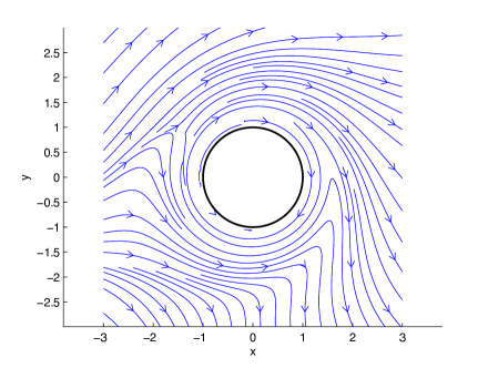
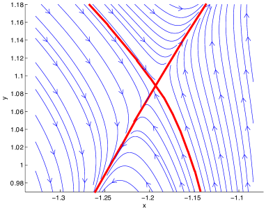
Figure 43: Magnetic field lines of an asymptotically uniform (weak electro-vacuum) magnetic field perpendicular to the black hole rotation axis [325, 328]. Left: the equatorial plane is shown ($xy$ Cartesian coordinates in units of $GM/c^{2}$, the horizon radius is indicated by circle). The magnetic intensity vanishes in two neutral X-type points near in the vicinity of a rapidly spinning Kerr black hole ($a/M=0.99$). Right: an enlarged detail of the structure around the magnetic null point.

As mentioned above, the magnetic field aligned with the rotation axis produces an asymptotically radial electric field, rather than a quadrupole field, as could be expected under similar circumstances in the classical electrodynamics. This difference is due to the combined gravito-magnetic effect of rotation and strong gravity of the black hole.

Magnetic fields misaligned with respect to the rotation axis exhibit very complex structure. Frame-dragging acts on the field lines and distorts them in the sense of black hole rotation. Non-zero magnetic flux still enters into the horizon and, naturally, the same magnetic flux has to emerge out of the black hole. Magnetic lines of an inclined (oblique) field are progressively wound up and the conditions suitable for magnetic reconnection are created [magnetic neutral points emerge in the ergosphere; cf. 327]. Let us emphasize that these effects occur due to purely geometrical action of strong (rotating) gravity, however, the presence of conducting (force-free) plasma of an accretion disk can lead to a similar structure of anti-parallel, rotationally distorted field lines [351]. The latter authors demonstrate the possibility of magnetically driven energy extraction from the black hole through the reconnection within the ergosphere.

We notice that magnetic null points emerge near the black hole, suggesting that magnetic reconnection can be initiated by the purely gravitomagnetic effect of the rotating black hole (Fig. 43). Indeed, this new mechanism has been proposed [325] in the context of particle acceleration processes in the ergosphere of rapidly rotating magnetized black holes. The induced electric component does not vanish in the magnetically neutral point, and hence it can accelerate the particles efficiently.

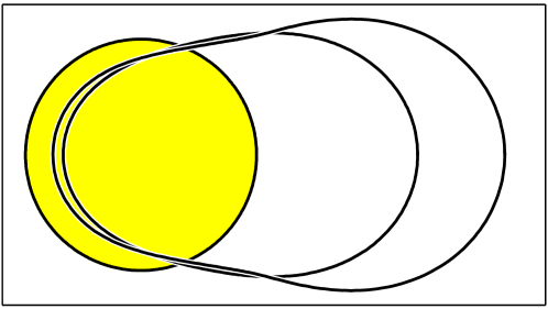
Figure 44: A cross-sectional area for the capture of magnetic flux by a rotating black hole. The three oval-shape curves correspond to different values of the black-hole angular momentum: spin $a=0$ (the cross-section has a form of circle of radius $2M$; its projection coincides with the black-hole horizon, indicated by yellow color); $a=0.95\,M$; and an extremely rotating Kerr black hole, $a=M$. The enclosed area encompasses the field lines of the asymptotically perpendicular magnetic field which eventually enters into the black hole horizon. This area grows with the black hole spin and its shape is distorted by the gravitomagnetic interaction (figure adapted from Dovčiak et al., , 2000).

As mentioned above, the magnetic field lines thread the horizon and become captured by the black hole if the orientation is mis-aligned with the rotation axis. The capture of magnetic field lines of the perpendicular field is seen in Fig. 44, where we plot the black hole effective cross-sectional area. The oval-shaped region is formed by end-points of those field lines at large spatial distance from the black hole ($r/M\rightarrow\infty$) which eventually cross the horizon and enter into the black hole. Starting from the circular shape for $a/M=0$ static case, the area in mention is increasingly deformed as the spin grows.

We can conclude that the frame/dragging effects on inclined magnetic magnetic fields lead to the emergence of magnetic neutral points and the associated reconnection. At the same time the magnetic flux is not rotationally expelled out of the black hole, so that the energy extraction via the Blandford-Znajek mechanism is possible even from a maximally rotating Kerr black hole. Finally, Fig. 45 shows the deformation imposed on the structure of the magnetic lines by the translatory boost onto the magnetic field. Again, this exhibits the purely geometrical effect which the black hole gravity has on the vacuum magnetic fields.

Surface charge can be formally defined by the radial component of electric field in non-singular coordinates [639],

$$\sigma_{\mathrm{H}} = \frac{B_{0}a}{4\pi\Sigma_{+}}\left[r_{+}\sin^{2}\theta-\frac{M}{\Sigma_{+}}\left(r_{+}^{2}-a^{2}\cos^{2}\theta\right)\left(1+\cos^{2}\theta\right)\right]$$ (179)

$$+\frac{B_{\perp}a}{4\pi\Sigma_{+}}\,\sin\theta\,\cos\theta\left[\frac{Mr_{+}}{\Sigma_{+}}+1\right]\left[a\sin\psi-r_{+}\cos\psi\right],$$

with

$$\psi=\phi+\frac{a}{r_{+}-r_{-}}\,\ln\frac{r-r_{+}}{r-r_{-}}\,\propto\ln(r-r_{+}).$$ (180)

For $a\ll M$,

$$\sigma_{\mathrm{H}}=\frac{a}{16\pi M}\left[B_{0}\left(1-3\cos^{2}\theta\right)+3B_{\perp}\sin\theta\,\cos\theta\,\cos\psi\right].$$ (181)

It should be noted that $\sigma_{\mathrm{H}}$ does not represent any kind of a real charge distribution. Instead, it is introduced by analogy with junction conditions for Maxwell’s equations in classical electrodynamics. The classical problem was treated in original works by Faraday, Lamb, Thomson and Hertz, and more recently in Bullard, [106] and Elsasser, [208]. It is quite enlightening to pursue this similarity to greater depth (see e.g. Karas and Budínová, [321], and references cited therein) despite the fact that this is purely a formal analogy, as pointed out by Punsly, [552].

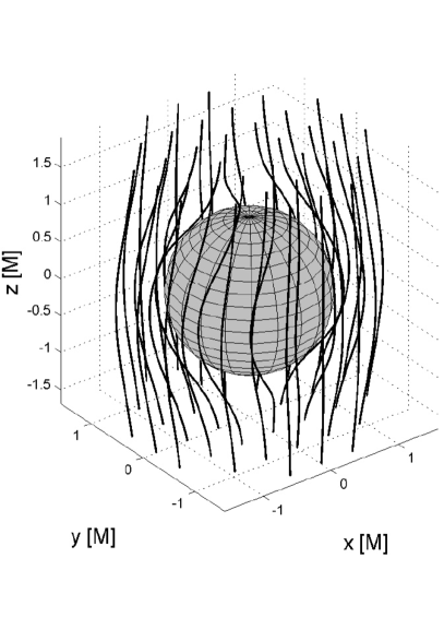
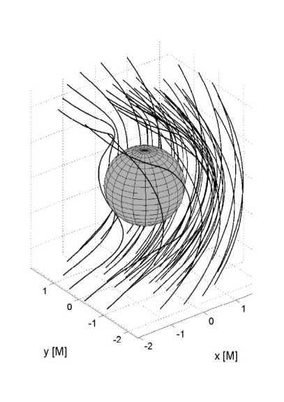
Figure 45: Two examples of organized (electro-vacuum) magnetic fields near a rotating black hole in 3D projection. Left: the case of an asymptotically uniform magnetic field aligned with the rotation axis (parallel to the direction of $z$-axis). Right: the effect of linear (translatory) boost, where the black hole moves along the $x$-axis (figure from Karas et al., 2012a, ).

So far we discussed test-field solutions of Einstein equations which reside in a prescribed (curved) spacetime. In the rest of this chapter we will briefly outline a mathematical procedure to construct exact solutions of mutually coupled Einstein–Maxwell equations [362]. Because this task can be rather complicated, astrophysically realistic results can be only obtained by numerical approaches. However, an important insight can be gained by using the simplified analytic solutions. We defer a brief mathematical exposition to this latter approach to Appendix 5.2.

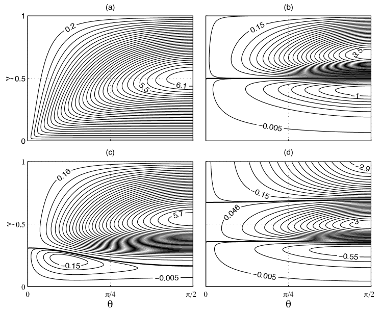
Figure 46: Contours of magnetic flux across a cap on the horizon (latitude angle $\theta$ is measured from the rotation axis) of a magnetized black hole: (a) $a=e=0$; (b) $a=1$, $e=0$; (c) $a=0.2$, $e=0$; (d) $a=-e=1/\sqrt{2}$ (electric charge and spin of the black hole). Here, $\gamma\equiv\left(1+\beta\right)^{-1}$, $\beta\equiv B_{0}M$. The horizontal separatrices (thick lines) correspond to extreme configurations, where the Meissner-type effect causes a complete expulsion of the magnetic field out of the black hole horizon. This figure (adapted from Karas and Budínová, 2000) illustrates strong-gravity effects on magnetic fields that do not occur in the weak-magnetic (test) field approximation, namely, the expulsion of the magnetic flux as a function of the intensity of the imposed magnetic field (notice the horizontal lines of separatrices, where the magnetic flux vanishes). Let us emphasize that, unlike the original discussion of the Meissner effect on weak magnetic fields, here we consider exact, asymptotically non-flat, electro-vacuum spacetimes of coupled Einstein–Maxwell fields.

It can be shown that the only static magnetized Kerr-Newman black hole is the one with the vanishing total charge $Q_{\rm{H}}$ and total angular momentum $J_{\rm{H}}$ [as defined by Komar’s integral relation; 332]. Let us remind the reader that these solutions are not asymptotically flat because the magnetic field does not disappear at large spatial distance from the black hole. Instead, the spacetime metric approaches the magnetic universe [429].

Fig. 46 shows the magnetic flux across the black hole hemisphere in the exact magnetized black hole solution. Four panels capture the topologically different configurations arising for different combinations of spin parameter $a$ and the electric charge $e$. By setting $\theta=\pi/2$, one obtains the flux across the entire hemisphere. The top-left panel (a) corresponds to the case of magnetized non-rotating (Schwarzschild–Melvin) metric ($a=e=0$) while (b) and (d) show two extreme configurations ($a^{2}+e^{2}=1$). In Fig. 46a the flux reaches maximum of $F=2\pi$ for $\gamma=0.5$ [see also 241, 321]. In other words, the flux is not a monotonic function of the magnetic-field parameter and it decreases when the field strength exceeds a certain critical value, depending on the interplay between the magnetic intensity, distribution of the flux across the horizon, and its surface. In terms of its $\beta$-dependence, the flux first concentrates to symmetry axis $\theta=0$ when $\beta$ increases from zero to unity, but than it spreads away from the axis of rotation. Let us note that this is an exemplary behaviour that occurs in exact solutions with strong magnetic fields but it diseappears in weak test fields.

3.3 Particle acceleration and jet launching near SMBH

Observations reveal that collimated outflows of matter are a generic phenomenon connected with certain types of astronomical objects. These jets exist on very different length scales and they are associated with sources ranging from stars to galactic nuclei – over nine orders of magnitude in the mass of the central source [see 54, 81, for authoritative reviews]. The nature of jets and the associated mechanism of jet formation, acceleration and disruption are very diverse, but they also exhibit common properties [142]. Unifying schemes have thus been proposed, initially motivated by observations. It has been speculated about analogies between electromagnetic processes that accelerate particles near pulsars [61] versus processes in magnetospheres of supermassive black holes [85, 292]. It is tempting to ascribe (part of) the differences, at least in case of AGN jets, to an unequal orientation of these objects with respect to the observer. The interest in this subject has been amplified by the discovery of relativistic motion in microquasars in our Galaxy [451, 294, 641] which have their well-known counterpart in extragalactic superluminal jets [713]. Excellent original articles reviewing the developments of our knowledge about jets are available, both for relevant stellar-scale objects in the Galaxy [512, 248] and for extragalactic jets [54, 648].

Different mechanisms have been proposed by which a black hole and its accretion disk can launch jets [639]. Firstly, an outflowing wind from the gaseous disk may create a bubble in an infalling rotating cloud; hot gas then makes the orifices and the jet is shot out. Secondly, the surface of a geometrically thick rotating accretion disk may form funnels and collimate the wind. Thirdly, magnetic field lines are anchored in the disk material, thus spinning due to the overall rotation which pushes plasma to create jets. Finally, magnetic lines thread the hole, which forces them to spin and push plasma outwards. The jets are presumably formed in the innermost regions of the source (within a few or a few tens of gravitational radii, $R_{g}$, from the centre) and then they emanate outwards along the rotation axis of the central object. The initial phase of the jet formation is sometimes called pre-collimation in the literature, in distinction to processes of subsequent collimation that operate in more distant regions (magnetic fields play most probably a major role in maintaining collimated outflows on their course; [113, 392, 84]. If we are interested in the contribution to the total radiation that originates near the compact object, this still remains beyond current observational limits (which are at about $10^{3}R_{\rm g}$ for extragalactic sources). However, this has recently been changed by the Event Horizon Telescope observations [203] that have utilized the mm-VLBI technique [87].

Several mechanisms of the jet initial pre-collimation have been proposed to operate at the launching site near SMBH, where strong gravity effects and the relativistic frame dragging operate: Abramowicz and Piran, [7] and Sikora and Wilson, [607] consider collimation inside a funnel of a luminous thick accretion disk. Material of the jet is in mutual interaction with the disk radiation which determines its terminal speed [538]. Since early 1980s the idea of the disk-like accretion flows at high accretion rates has evolved to an intricate form but the general scheme of jets flowing along the disk axis under radiative drag remains viable. The model has been advanced by detailed quantitative calculations of the jet acceleration both within the framework of the hydrodynamic [383] and the test particle approximations [427, 660]. These calculations confirm the importance of the disk radiation on the jet dynamics. de Felice and Curir, [172] constrained the rate of change of energy and angular momentum of an interesting special family of particle trajectories that spiral along the axis. They do find collimation but the physical nature of dissipative processes that cause the loss of particle energy and angular momentum remains unclear. Purely geodesic motion in the Kerr geometry does not contribute to collimation except when the existence of a hypothetical naked singularity in the centre is accepted [73, 583].

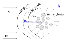
Figure 47: The particle acceleration operates across the shock discontinuity when a relativistic jet interacts with a passing star. Left panel: a double bow-shock structure arises due to a stellar wind interacting with a supersonic jet. The jet and the wind shocked regions are separated by a contact discontinuity. The shocked matter flows downstream, i.e., away from the shock apex. $D_{j}$ and $D_{w}$ denote the size and thickness of the jet and the wind bow-shock downstream regions, respectively. Right panel: the efficiency of the mechanism increases dramatically as a dense star-cluster happens to cross the jet flow line (Araudo et al., 2013, 2017).

Furthermore, stars can occasionally transit across the jet and produce shocks [53]. The interaction provides a scenario to address non-thermal processes. A double bow-shock structure forms and particles become accelerated via DSA mechanism. Individual encounters have a limited effect, however, dense clusters of massive stars can truncate the jet as the cluster crosses the jet line near the jet launching region. Araudo and Karas, [28] considered the effects of interaction of jets in Active Galactic Nuclei when they encounter multiple obstacles, namely, stars in Nuclear Star Cluster surrounding the nucleus and globular clusters passing across the inner jet (Fig. 47).

It may be interesting to note that the interaction between the accretion disk, jet, and star of the Nuclear Star Cluster can greatly influence that mode of accretion, the jet emanation, and the radiation produced by the two components. Collisions of the star with an accretion disk can (quasi-)periodically modify the radiation flux from the source and give us information about the evolution of the orbit. Its orientation with respect to the observer will be affected by general relativistic effects (periastron shift, Lense–Thirring precession) and corresponding modulation with specific periodicities may provide us with the evidence of the black hole in the core [333]. The model of a star orbiting a SMBH has been considered by several authors in different situations. A mechanism of the tidal capture of a star by a black hole has been discussed [291, 557, 496].

Star-disk direct hydrodynamical collisions offer another possibility [632, 542]. Ostriker, [507] proposed that the collisions could enhance the viscous drag on the accretion disk. Zentsova, [714] calculated a temperature profile of a bright spot which is created in the place were the star crashes through the disk. She estimates that the maximum local intensity is in the UV band. The collisions are highly supersonic: Mach number of the order $10^{2}$–$10^{3}$. Assuming that the core of AGN is embedded in a dense star cluster, Zurek et al., [721] estimate that the amount of the disk material swept out of the disk by stars’ passages is enough to form the gas clouds of the broad line region. Syer et al., [632] calculate time-scales for the evolution of the orbital parameters in the Newtonian approximation: star-disk collisions result in circularization of the orbit, the inclination is reduced and the star becomes a part of the disk. Vokrouhlický and Karas, [661] have obtained similar results for a star moving in the field of a Kerr black hole. In contrast to the Newtonian case, the probability that the star will be captured by the black hole is now higher because subsequent collisions can set the star in an unstable orbit which ends in the black hole. Let us note that the effective cross-section for star-disk interaction can be significantly enlarged in case of a magnetic star. This may then lead an increased drag; for a textbook account of the subject, see Lipunov, [386] and Romanova et al., [568].

4 Unification of accreting black holes across the mass scale

“It’s a bit like playing chess with nature as your opponent. You make a good move, but nature counters with half a dozen new ones."

— Eleanor Margaret Burbidge

4.1 Fundamental plane of black hole activity

Processes related to black hole accretion, which we described in previous sections, are not exclusively related to AGN physics only. Black holes themselves are very simple objects characterised by their mass and rotational momentum (electric charge is probably unimportant for astrophysical black holes in practice). That’s why it is widely believed that similar processes occur around black holes across their mass range from a few masses of Sun in stellar-collapsed black holes in X-ray binaries (XRBs) up to billions of Solar masses in the most massive AGN.

The unification between the supermassive and stellar-mass black holes became first evident from an empirical extension of the XRB relation between the radio and X-ray luminosity to AGN, the so called fundamental plane of black-hole activity [433]. Figure 48 shows the dependence of the radio luminosity on the X-ray luminosity and the black-hole mass for different kinds of objects, including XRBs (circles), low-accreting supermassive black holes (Sgr A* and M 32, shown by squares) as well as highly-accreting Seyferts (triangles) and quasars (stars). The color denotes the central black-hole mass (black represents mass corresponding to stellar masses, i.e. lower than 100 M_⊙, while the other colors represent ranges for masses of the super-massive black holes in galactic centres). The found correlation from the multivariate regression analysis by Merloni et al., [433] was:

$$\log L_{\rm R}=(0.6\pm 0.11)\log L_{\rm X}+(0.78^{+0.11}_{-0.09})\log M+7.33^{+4.05}_{-4.07}.$$ (182)

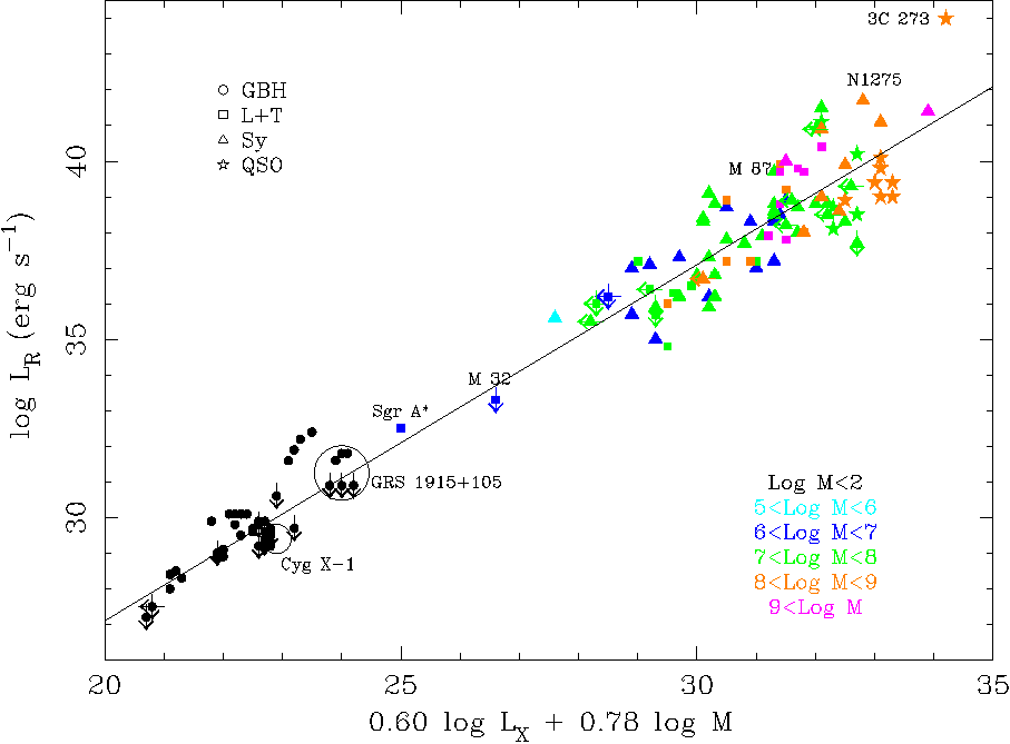
Figure 48: Fundamental plane of black hole activity showing a relation between the radio and X-ray luminosity with mass for different kinds of black holes [from 433].

The radio luminosity plays an important indicator for the jet presence, while X-rays are connected with the accretion. The fundamental plane of the black-hole activity thus observationally demonstrated the relation between the accretion physics and the jet launching mechanisms. Moreover, it showed that the relation is similar for XRBs and AGN, i.e. for objects with entirely different masses, suggesting that the jet models are scale-invariant, as proposed, e.g., by Heinz and Sunyaev, [286]. Moreover, the found correlation is quantitatively consistent with the advection-dominated accretion flow (ADAF) rather than the standard accretion disk scenario. This indicates that the jet is a prominent feature mainly during this kind of accretion flow that is related with a sub-Eddington accretion rate, and the fundamental plane is appropriate for sources in this so-called hard state.

The fundamental plane has shown similarities between XRBs and AGN and has opened the way to the unification of black-hole activity across the mass range. Understanding what is common and what is inherently different between these two classes will allow us to use the knowledge of one black-hole kind to the other and better understand the black-hole physics in general. What is clearly different between the XRBs and AGN is the characteristic time scale, at which the accretion flow evolves. While for XRBs several changes of their accretion modes have been detected (and different associated spectral states have been identified, see next Section for more details), AGN probably remain in the same accretion state during monitoring over years and decades. Several observational phenomena that are related with the XRB spectral states are, however, observed for AGN as well, including large variability and outflows in the form of jets and winds. Also, in the other way round, some XRB spectra revealed the features more typical for AGN. An example could be V404 Cyg in its recent outburst, where Motta et al., [463] revealed the presence of winds and large obscuration analogical to AGN spectra. The next sections are devoted to describe the spectral states of XRBs and to discuss possible analogy of spectral states in AGN.

4.2 Spectral states: AGN vs. microquasars?

The XRB spectral state can be quite well defined by the intensity and spectral hardness (ratio between hard and soft X-ray flux) in the so-called hardness-intensity diagram (HID) [227]. The soft X-ray band is dominated by the accretion-disk thermal emission. Thus, sources in the “high/soft” state (HSS) produce most emission in the form of thermal radiation. Oppositely, sources lacking the accretion-disk thermal emission are dimmer and harder and the state is referred to as “low-hard” state (LHS). It is believed that sources in the LHS have their accretion disk truncated at a further radius while in HSS the disk innermost edge coincides with the innermost stable circular orbit at 1–6 $GM/c{{}^{2}}$ depending on the black hole spin. The X-ray corona is weak in HSS, while it is strong in LHS.

The spectral states of X-ray binaries evolve very rapidly [188], they can change in order of hours to days. An intriguing property is an observed hysteresis in HID. During a typical outburst, the source gets brighter by several orders of magnitude, but its hardness does not change significantly [see, e.g., 226]. Then, either the outburst fails and the source goes back to quiescence, or the source very rapidly moves to the HSS and thermal emission starts to prevail in the spectrum. The transition back from soft to hard always happens when the luminosity is much lower. Several explanation of this hysteresis behaviour were proposed [121, 611, 440, 535, 144], but none has been widely accepted as the unique scenario.

With the XRB spectral states, several observational phenomena are related. Large variability (rms of order of a few tens of percent) is observed in the hard state while it diminishes in the soft state [298]. Interesting timing features occur during the spectral transitions when the variability suddenly drops. The power spectra reveal different kinds of quasi-periodic oscillations [see, e.g., 59]. Also the jet production is closely associated with the spectral states [227]. A persistent jet is present in the hard state while it disappears after the transition to the HSS. Ponti et al., [543] showed that XRBs in the soft state produce equatorial winds instead of the jets. Only sources in the so-called “very-high state” (or “steep-powerlaw state”) can still produce blobs of relativistically accelerated matter ejected from the source in the polar (jet) direction. These ballistic jets are highly relativistic (have very large Lorentz factor) and unstable (they never built a persistent jet). Narayan and McClintock, [473] showed that the strength of the ballistic jets is correlated with the BH spin, while the correlation between the spin and the radio power of persistent jets was found to be dubious [228].

The spin - jet power relation has significant implication also for AGN physics. From large extragalactic surveys, it was shown that $\sim 10\%$ of AGN are radio-loud [339], while the majority is radio-quiet. There have been long discussions what physical processes lead to this distinction, the spin paradigm being one of the most favourite physical interpretation [455, 606]. However, in analogy to XRBs, it was suggested by Koerding et al., 2006b [350] and Svoboda et al., [630] that the observed radio dichotomy may be explained by AGN spectral states similar to those in XRBs. Prominent jets extending to extra-galactic space are observed in several nearby AGN, such as M87 [314]. Jet emission represents a significant contribution in radiation observed from low-luminosity AGN, for which the radio loudness was found to be anti-correlated with the Eddington ratio [see, e.g., 296, 517, 606, 308], qualitatively confirming the possible analogy with the jet presence in the XRB “low-hard” state. Indeed, it was proposed in the past that different kinds of AGN may correspond to different spectral states similar to XRBs [see, e.g., 350, 422, 612].

Direct comparison of AGN with XRBs is difficult mostly because of the largely different mass ($M\approx 10^{5-10}\,M_{\odot}$) that determines both the size and the time scales. The size scale affects the temperature of the accretion disk because the disk inner edge is located further from the BH singularity in AGN than in XRBs. The AGN thermal emission thus dominates in the UV band [404, 377], which is, however, difficult to observe due to large interstellar and intergalactic absorption. In addition, AGN are not isolated. They are surrounded by the whole galaxy whose hot stars significantly contribute to the total UV emission coming from the active galaxy. Because of the observational difficulties, the UV spectrum is one of the least understood part of AGN spectral energy distribution (SED). Although the apparent excess (Big Blue Bump) is usually associated with the thermal emission from the accretion disk. It was, however, noticed already by Elvis et al., [211] that the quasar spectra cannot be generally described by the thermal blackbody emission of a thin accretion disk. This lead to the hypothesis that AGN UV and soft X-rays need to be explained by an additional Comptonization component that is unique for AGN and not present for XRBs [181, 180].

The other complication related to the mass is the different time scale of AGN and XRBs. A complete cycle of an XRB outburst from quiescence through hard state to soft state is of the order of a few hundred days [560, 188]. AGN with significantly larger black holes have the time scales proportionally larger. It is therefore impossible to wait for a spectral change in an AGN. Even the shortest independently estimated timescales for an AGN phase is $10^{5}$ years [581]. The only chance is thus to detect a source during the very fast transition, such as the “hard-to-soft” transition, that takes only hours in XRB and that would correspond to years in AGN. Some changing-look AGN were indeed proposed to be candidates of spectral changes [372, 401, 420], but in some cases other interpretations have also been proposed [see e.g. 432]. Most AGN are not variable in X-rays by a factor larger than a few over decades [620], suggesting that they remain in the same spectral state. Only a large homogeneous AGN sample can populate the HID with a sufficient number of sources.

A seminal work on an AGN HID was done by Koerding et al., 2006b [350]. They generated a disk-fraction luminosity diagram for a large sample of quasars from the Sloan Digital Sky Survey [9] and from archival X-ray measurements from the ROSAT All-Sky Survey [659]. They showed that radio-loud AGN lack the thermal emission and their luminosity is dominated by X-rays from non-thermal processes. However, the SDSS sample does populate only high-luminosity part of the diagram with the sensitivity limit ($L\approx 10^{44}$ erg s^-1), not including the low-luminosity AGN. Their results could also be affected by the limited bandpass of the ROSAT/PSPC detector, and by the non-simultaneity of the data if the observed flux is significantly variable. However, a recent work by Svoboda et al., [630] revealed the same trend for AGN sample based on simultaneous UV and X-ray observations obtained by XMM-Newton. The sensitivity of XMM-Newton measurements allowed them to study low-luminosity sources as well. They found that their radio loudness is also related with the UV/X-ray spectral hardness, but the precise measurement of the spectral hardness is compromised by generally unknown host-galaxy contamination that affects more UV than X-rays. Therefore, the low-luminosity sources appear softer than would be their intrinsic nuclear emission. This is apparent from the comparison between AGN and XRB HID (see fig. 49), and was shown by Svoboda et al., [630] that the effect of host galaxy is indeed the most likely reason for this discrepancy.

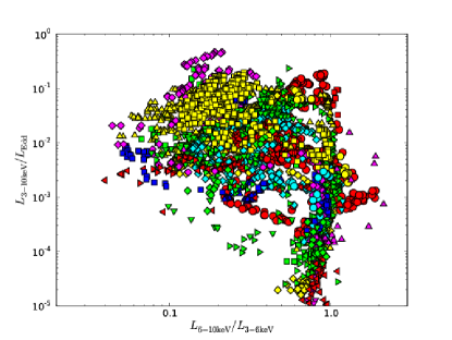
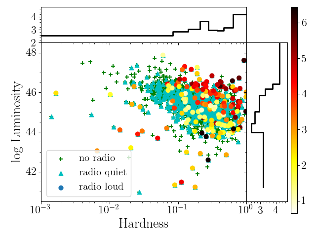
Figure 49: Comparison of hardness-intensity diagrams for an XRB sample in the left panel [188] vs. AGN sample on the right [630]. Different colors in the XRB plot represent different sources. The color in AGN plot denotes the relative radio loudness. The radio loudness per hardness bin is shown in the upper histogram (for radio-loud sources only), revealing the increase of radio loudness towards hard states. The side histogram shows the relative radio loudness per luminosity bin.

The host-galaxy decomposition is difficult in the absence of very high spatial-resolution observations that are available only for the nearest galaxies. One possible way is a detailed modelling of the AGN SED [see e.g. 295, 297, and references therein]. This has been done so far for only nearby AGN, and there is not yet a fully accepted consensus on the UV emission. While Ho, [297] concluded that these sources completely lack the UV emission from the nucleus, Maoz, [406] found a significant contribution that can be associated with the nuclear activity. Other possible method could be employed for data with available long-term monitoring. While the AGN flux is inherently variable, the host-galaxy emission can be supposed as constant contribution to the total flux [493]. The proper decomposition of the host galaxy from AGN emission is crucial for a more detailed study of low-luminosity (and thus very often low-accreting) sources.

Based on the qualitative agreement between the XRB and AGN spectral states, it was suggested by Koerding et al., 2006b [350] and Svoboda et al., [630] that AGN spectral states may explain the observed radio dichotomy, i.e. a distinction between radio-quiet and radio-loud AGN [339]. Previously, it was proposed that the black hole spin is the important parameter [455, 606]. However, we know from XRBs that the jet production does not occur in the HSS (when the matter gets to the innermost stable circular orbit), but the persistent jets only appear in the LHS (when the accretion disk is believed to be truncated). In this sense, the spectral state (accretion mode) might play a prime role whether the jet is launched or not, and then the effect of the spin will be imprinted in the power of the jet.

If the jet is related to the spectral state, it should be then possible to track the radio-morphology evolution in the HID. The previous morphological classifications, such as one by Fanaroff and Riley, [224], distinguishing core- and lobe- dominated radio emission, may be related with the interstellar medium in the host-galaxy rather than to the intrinsic jet evolution [244, 452]. This implies that high-resolution and high-sensitive data from jet cores will be essential in understanding the fundamental physical parameters of black hole activity [see, e.g., 519]. The planned extension of the VLA Sky Survey (VLASS), ASKAP/EMU in the southern hemisphere or APERITIF/WODAN in the north [for a review see e.g. 495], and finally the SKA radio interferometer [175], will allow more detailed studies of AGN jet morphologies.

4.3 Very high energy particles and photons

The Earth upper atmosphere is continuously bombarded by very-high energy particles and gamma-ray photons, which have been originally discovered in an indirect manner, via balloon experiments performed at the beginning of 20th century [287, 30]. According to the widely accepted scenario for explaining the cosmic-ray production, energetic nucleonic particles are produced via diffusive-shock acceleration mainly in supernova remnants. The particles remain trapped in the tangled Galactic magnetic field for $~{}10^{7}$ years (at GeV energies) until they eventually escape or interact with other nuclei in the interstellar medium.

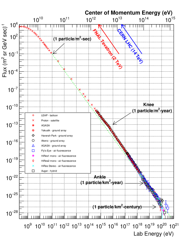
Figure 50: The spectrum of cosmic ray particles of different chemical composition is plotted against several limits of particle accelerator experiments. Relatively small departures from the uniform power-law dependence (the “knee” and the “ankle”) provide important clues about the acceleration mechanisms and the composition of cosmic rays (figure from Hanlon, [280]).

Highly energetic electrically charged particles of cosmic origin are usually denoted as cosmic rays, and despite a great progress their exact origin still remains very puzzling [223]. Charged particles of cosmic rays and cosmic gamma rays are mutually connected by physical mechanisms of their origin and propagation. To date there are multiple candidates for the sources within the Galaxy and further out, however, it is believed that violent processes in the vicinity of compact stars and supermassive black holes play the main role in their production. At the very highest energies ($>10^{19}$ eV) these particles are mostly extra-galactic in origin, and possibly correlated with the structure of active galaxies [540, 316].

Active Galactic Nuclei are thus promising potential sources of Ultra High Energy Cosmic Rays (UHECRs), which are particles having an energy of $\sim$100 EeV. These mysterious messengers arrive on Earth from outside the Galaxy, but their origin remains unknown [540]. Radiogalaxies are a subclass of AGN where jets are detected at radio frequencies, which in turn are classified as type I and type II Faranoff–Riley (FR) galaxies. In this context high resolution radio data provide a very powerful piece of information to study particle acceleration and to determine the nature of amplified magnetic field. In both cases, jets moving in the intergalactic medium are believed to produce shock waves where particles accelerate via the diffusive shock acceleration mechanism [DSA; 57]. In fact, DSA appears to be the best established process to accelerate particles in astrophysical sources where shock waves are present: particles diffuse back and forth across the shock front and gain energy in each crossing. Therefore, extended time is required to accelerate the most energetic cosmic rays unless the magnetic field around the shock is amplified. The amplified turbulent field scatters particles, so that they cross the shock more frequently and achieve high energy in the available time. The current state of the art, however, is a mainly phenomenological scenario where the acceleration process finishes at the moment when particles start radiating their energy (or when they can escape from the source). The underlying assumption behind this scenario is that the magnetic field persists over long distances all the way downstream of the shock. However, it has been shown [26] that the magnetic field must be highly discrete to explain the thin radio emission in the jet termination region of some quasars. This result has important consequences for determining the maximum energy of particles accelerated up to about 1 TeV and the problem of UHECR acceleration remains open.

The observed energy spectrum of high-energy cosmic rays is a power-law that exhibits a monotonic fall-off [280, 631], as seen in fig. 50. The energy spectrum is an almost precise, uniform power-law decay. In order to gain sufficient Signal-to-Noise ratio at the highest energies one needs enormous collecting area of the instrument. Multiplying the flux by a power-law proportionality with the energy power about 2.7 flattens the spectrum almost precisely below $10^{16}$ eV. There are additional features at higher energies that we can call the “knee” and the “ankle”. In fact, the cosmic ray spectrum resembles a leg; we can imagine the knee (in the second break of the power law), and the ankle (in the third break in the power law) in the plot shape.

Ultra-high energy photons may arise by a number of processes and they likely contribute to the total flux of cosmic rays. In 1966, Greissen, Zatsepin, and Kuzmin [273, 709] predicted that the interaction of charged particles with the low-energy relic photons of cosmic microwave background radiation will lead to the suppression of the cosmic ray flux at energy above $\simeq 5\times 10^{19}$ eV for sources beyond the distance of a few Mpc (GZK limit). However, see Bird et al., [74].

Very-high energy gamma-rays arise in non-thermal processes by interactions of accelerated, electrically charged particles with the surrounding environment in rather extreme physical conditions, such as supernova remnants, and the immediate vicinity of black holes in AGN. The radiation processes leading to gamma rays are associated with accelerated charged particles, although gamma-rays could be potentially created also by more exotic mechanisms, such as the decay of dark matter particles.

Below GeV energies the cosmic rays are predominantly of solar origin, however, the cosmic ray spectrum extends much up to $\sim 10^{20}$ eV. Because these are electrically charged particles, cosmic rays become deflected by the Galactic and extragalactic magnetic fields, which randomize their direction at the point of entry in the Earth atmosphere. On the other hand, unlike the charged cosmic rays, gamma-ray photons are not affected by magnetic fields, and so they can be traced back to their original sources at least in principle. It has been proposed that TeV photons could originate from the decay of pions that arise in interactions of protons $\gtrsim 10\,$TeV energies [239].

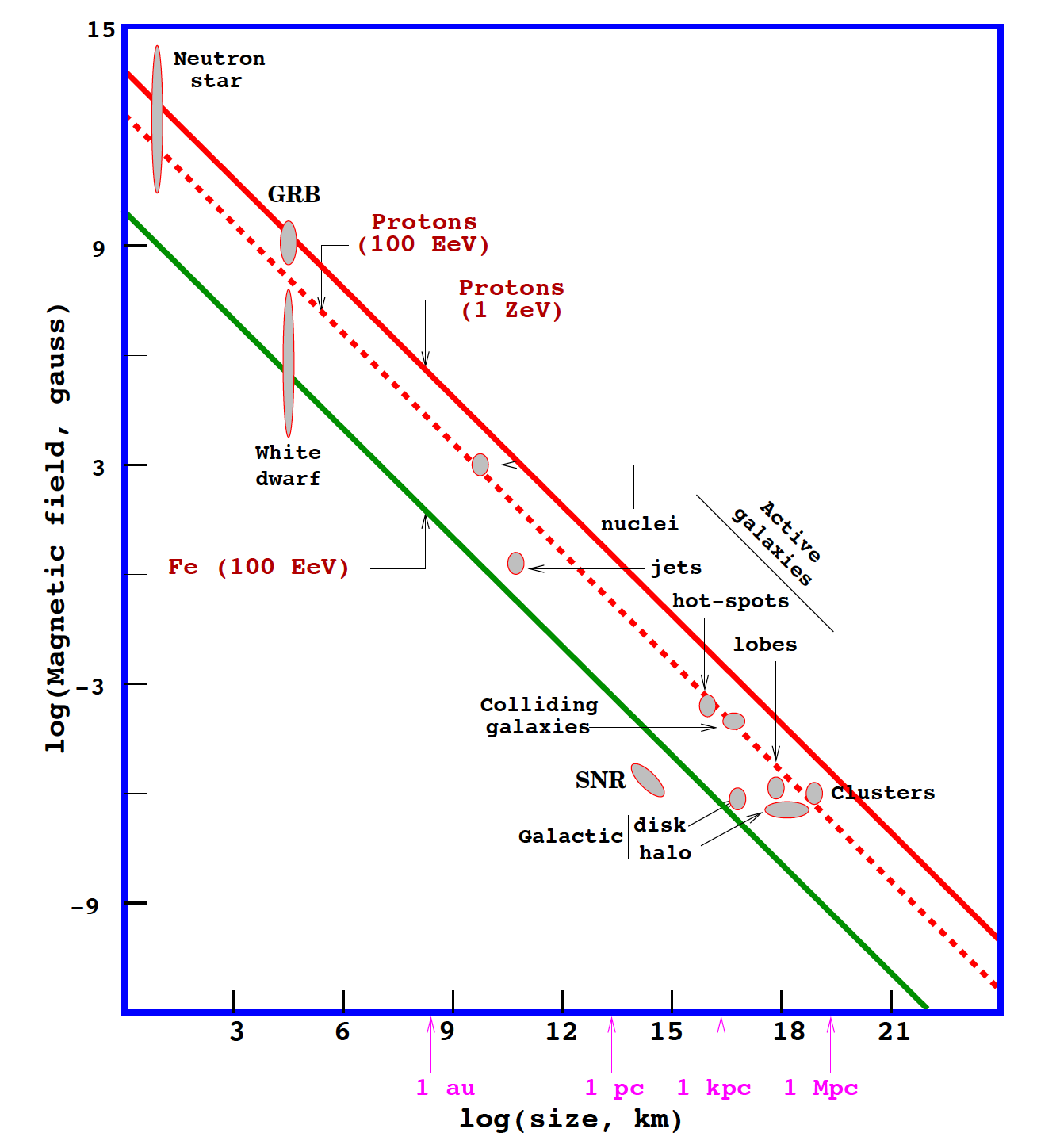
Figure 51: The Hillas diagram constrains the possible sites of cosmic rays depending on the characteristic size of the source and the magnetic field intensity confined within its volume. Diagonal lines indicate the maximum energy above which the source is unable to accelerate cosmic rays of a given chemical composition. In particular, the attainable energy for protons of $10^{20}$ eV (so far the highest value reported observationally) is shown by two red lines corresponding to different values of energy $E$ (or the shock velocity $\beta$; (see the text for further details). An analogous line for the case of iron atoms would be placed parallel towards bottom left (green). Various cosmic sources can produce cosmic rays above the limits of what current laboratory accelerators achieve (the position of the Large Hadronic Collider (LHC) would be placed around the size 1 km and the magnetic intensity $\sim 10^{5}$ G. Figure drawn by Murat Boratav.

Neutrinos are a very interesting aspect of cosmic ray production even if they are not considered as a separate component of this phenomenon (we do not have a neutrino spectrum). They propagate along a straight path and, thanks to their small cross-section, neutrinos can traverse enormous matter depth without experiencing any interaction or absorption. They can thus serve as excellent messengers from extragalactic sources, where they are produced by hadronic processes due to the acceleration of matter to high energies [316]. Neutrinos are also produced by cosmic rays interacting with the cosmic microwave background. On the Earth, neutrinos can emerge in cosmic ray showers and they can be detected via methods of particle physics, such as Pierre Auger Observatory [115], and ANTARES and the Ice-Cube experiments [11, 12]. The neutrino trajectory between the source and the observer is straight and unperturbed for the neutrinos produced within the Galactic and the extragalactic sources. This has enabled to associate the neutrino with specific AGN and study the radio/gamma-ray properties of blazars, both BL Lac sources [TXS 0506$+$056; 96] as well as FSRQs [PKS 1502$+$106; 98]. However, the cosmic neutrino background may be affected by the gravitational lensing within the galaxy cluster and galaxy halos since a fraction of cosmic neutrinos has likely become already non-relativistic with larger deflection angles. This can then induce anisotropies in the cosmic neutrino background with the features including Einstein rings that, however, behave chromatically for massive neutrinos depending on the cosmic neutrino momentum spectrum [690]. In terms of the Galactic neutrinos that originate within core-collapse supernovae, there is a curious possibility of the supernova neutrino lensing by the Sgr A* SMBH in case the supernova is nearly aligned along the Earth–Galactic center connection [430]. However, these events are extremely rare: two orders of magnitude enhancement of neutrino flux is likely to occur once every few billion years, and one order of magnitude enhancement can occur once every 250 million years. A more probable event is the detection of the difference in the arrival time by as much as 20 seconds in case the supernova is not perfectly aligned with the Galactic center, but this is expected to occur still only once 29 million years [430].

Besides supernova remnants, which appear to be highly probable sources in the Milky Way, very-high energy gamma rays can be efficiently generated in pulsar wind nebulae, in pulsar magnetospheres, and jets in microquasars. Among extragalactic objects, nuclei of active galaxies and starburst galaxies are likely sources. Gamma-ray bursts (GRBs) are expected to produce very-high energy gamma-rays in shocks via the synchrotron and inverse Compton processes in jets.

In 1984, Hillas [290] formulated an ingenuous and general criterion for the acceleration of charged cosmic ray particles of atomic number $A$ up to high energy $E_{\rm max}$ (see fig. 51). Namely, the characteristic condition that connects the intensity of the magnetic field $B$ and the acceleration region size $L$ is determined by the Larmor radius, which can be visualized in the Hillas relation [508, 129, 171, 170, 18],

$$E_{\rm max}\simeq 10^{18}Z\beta\frac{L}{\rm kpc}\frac{B}{\mu\rm G}\;{\rm eV},$$ (183)

where $\beta c$ is the characteristic velocity. It turns out that only the most powerful AGN are able to accelerate protons to ultra-high energies, nevertheless, the acceleration of heavier nuclei is possible in more abundant Seyfert galaxies [551]. The Hillas limit is thus an upper limit on the energy that particles can achieve, quite independent of the particular acceleration mechanism although the shock acceleration appears to be among the most promising scenarios.

5 Appendix

“The beauty of mathematics only shows itself to more patient followers."

— Maryam Mirzakhani

5.1 Mathematical formalism of spin coefficients

Tensorial variables are projected onto a complete vector basis at each point of the curved spacetime [487, 250]. It has proven to be extremely useful choice with a far-reaching impact, also in the context of gravitational waves [638], however, here we confine ourselves to electromagnetism near black holes in vacuum [347, 69]. Besides other features the spin-coefficient formalism is attractive especially because it leads to a set of first-order equations.

The vectorial basis can be conveniently chosen as a complex null tetrad, $l^{\mu}$, $n^{\mu}$, $m^{\mu}$, $\bar{m}^{\mu}$, satisfying the conditions $l_{\nu}n^{\nu}=1$, $m_{\nu}\bar{m}^{\nu}=-1$ (all other combinations vanish). A natural correspondence with an orthonormal tetrad reads

$$e_{(0)}=\frac{l+n}{\sqrt{2}},\quad e_{(1)}=\frac{l-n}{\sqrt{2}},\quad e_{(2)}=\frac{m+\bar{m}}{\sqrt{2}},\quad e_{(3)}=\frac{m-\bar{m}}{\Im\,\sqrt{2}}.$$ (184)

Although this seems to be more a topic of theoretical physics than astrophysics, we will briefly expose the relevant mathematics; it has proved to be very useful in deriving and elucidating the gravitational effects on electromagnetic fields in their mutual interaction. Let us emphasize that our overview is highly incomplete and focused only to a few selected aspects.

Let us note that the adopted definition of the null tetrad is not unambiguous; the following three transformations maintain the tetrad properties:

$$l \rightarrow l,\quad m\rightarrow m+al,\quad n\rightarrow n+a\bar{m}+\bar{a}m+a\bar{a}l;$$ (185)

$$n \rightarrow n,\quad m\rightarrow m+bm,\quad l\rightarrow l+b\bar{m}+\bar{b}m+b\bar{b}n;$$ (186)

$$l \rightarrow \zeta l,\quad n\rightarrow\zeta^{-1}l,\quad m\rightarrow e^{\Im\psi}m;$$ (187)

with $\zeta$, $\psi\in\Re$.

Instead of six real components of $F_{\mu\nu}$, the framework of the null tetrad formalism describes the electromagnetic field by three independent complex quantities,

$$\Phi_{0} = F_{\mu\nu}l^{\mu}m^{\nu},$$ (188)

$$\Phi_{1} = \textstyle{\frac{1}{2}}F_{\mu\nu}\left(l^{\mu}n^{\nu}+\bar{m}^{\mu}m^{\nu}\right),$$ (189)

$$\Phi_{2} = F_{\mu\nu}\bar{m}^{\mu}n^{\nu}.$$ (190)

It can be checked that the backward transformation has a form

$$F_{\mu\nu}=\Phi_{1}\left(n_{[\mu}l_{\nu]}+m_{[\mu}\bar{m}_{\nu]}\right)+\Phi_{2}l_{[\mu}m_{\nu]}+\Phi_{0}\bar{m}_{[\mu}n_{\nu]}+c.c.$$ (191)

The Newman–Penrose formalism defines the following differential operators:

$$D\equiv l^{\mu}\partial_{\mu},\quad\delta\equiv m^{\mu}\partial_{\mu},\quad\bar{\delta}\equiv\bar{m}^{\mu}\partial_{\mu},\quad\Delta\equiv n^{\mu}\partial_{\mu}.$$ (192)

Furthermore, Newman and Penrose, [487] introduce a set of spin coefficients (also called Ricci rotations symbols), which have been customarily denoted as follows,

$$\alpha = -\textstyle{\frac{1}{2}}\left(n_{\mu;\nu}l^{\mu}\bar{m}^{\nu}-\bar{m}_{\mu;\nu}m^{\mu}\bar{m}^{\nu}\right),$$ (193)

$$\beta = \textstyle{\frac{1}{2}}\left(l_{\mu;\nu}n^{\mu}m^{\nu}-m_{\mu;\nu}\bar{m}^{\mu}m^{\nu}\right),$$ (194)

$$\gamma = -\textstyle{\frac{1}{2}}\left(n_{\mu;\nu}l^{\mu}n^{\nu}-\bar{m}_{\mu;\nu}m^{\mu}m^{\nu}\right),$$ (195)

$$\epsilon = \textstyle{\frac{1}{2}}\left(l_{\mu;\nu}n^{\mu}l^{\nu}-m_{\mu;\nu}\bar{m}^{\mu}l^{\nu}\right),$$ (196)

$$\kappa = l_{\mu;\nu}m^{\mu}l^{\nu},\qquad~{}~{}\lambda=-n_{\mu;\nu}\bar{m}^{\mu}\bar{m}^{\nu},$$ (197)

$$\rho = l_{\mu;\nu}m^{\mu}\bar{m}^{\nu},\qquad\mu=-n_{\mu;\nu}\bar{m}^{\mu}m^{\nu},$$ (198)

$$\sigma = l_{\mu;\nu}m^{\mu}m^{\nu},\qquad\nu=-n_{\mu;\nu}\bar{m}^{\mu}n^{\nu},$$ (199)

$$\tau = l_{\mu;\nu}m^{\mu}n^{\nu},\qquad~{}\pi=-n_{\mu;\nu}\bar{m}^{\mu}l^{\nu}.$$ (200)

Despite that this is large number of variables the notation has turned out to be extremely practical. The best way is to demonstrate the usefulness of the formalism with examples.

We can write the null tetrad for Schwarzschild metric [see 347, 69]. The metric is then written in the form

$${\,\rm d}s^{2}=\left(1-\frac{2M}{r}\right){\,\rm d}t^{2}-\left(1-\frac{2M}{r}\right)^{-1}{\,\rm d}r^{2}-r^{2}{\,\rm d}\theta^{2}-r^{2}\sin^{2}\theta{\,\rm d}\phi^{2}.$$ (201)

The appropriate null tetrad is then given by

$$l^{\mu} = \left([1-2M/r]^{-1},1,0,0\right),$$ (202)

$$n^{\mu} = \left(\textstyle{\frac{1}{2}},\textstyle{\frac{1}{2}}[1-2M/r],0,0\right),$$ (203)

$$m^{\mu} = \frac{1}{\sqrt{2}\,r}\left(0,0,1,\Im\sin^{-1}\theta\right).$$ (204)

An arbitrary type-D spacetime (e.g. the Schwarszchild metric) allows to set $\kappa=\sigma=\nu=\lambda=0$. In particular, for the Schwarzschild metric the explicit form of non-vanishing spin coefficients is:

$$\rho=-\frac{1}{r},\quad\mu=-\frac{1}{2r}\frac{1}{1-2M/r},\quad\alpha=-\beta=-\sqrt{2}\,r\cot\frac{\theta}{2},\quad\gamma=\frac{M}{2r^{2}}.$$ (205)

Maxwell’s equations now adopt an elegant form

$$(D-2\rho+2\epsilon)\Phi_{1}-(\bar{\delta}+\pi-2\alpha)\Phi_{0} = 2\pi J_{l},$$ (206)

$$(\delta-2\tau)\Phi_{1}-(\Delta+\mu-2\gamma)\Phi_{0} = 2\pi J_{m},$$ (207)

$$(D-\rho+2\epsilon)\Phi_{2}-(\bar{\delta}+2\pi)\Phi_{1} = 2\pi J_{\bar{m}},$$ (208)

$$(\delta-\tau+2\beta)\Phi_{2}-(\Delta+2\mu)\Phi_{1} = 2\pi J_{n}$$ (209)

with $J_{l}=l_{\mu}(j^{\mu}+\Im\mathcal{M}^{\mu})$, $J_{m}=m_{\mu}(j^{\mu}+\Im\mathcal{M}^{\mu})$, $J_{\bar{m}}=\bar{m}_{\mu}(j^{\mu}+\Im\mathcal{M}^{\mu})$, and $J_{n}=n_{\mu}(j^{\mu}+\Im\mathcal{M}^{\mu})$. These are four equations for three complex variables.

Furthermore, Teukolsky, [638] derived the following general form of Maxwell’s equations:

$$\Big{[}(D \!\!-\!\! \epsilon+\bar{\epsilon}-2\rho-\bar{\rho})(\Delta+\mu-2\gamma)$$ (210)

$$-(\delta-\beta-\bar{\alpha}-2\tau+\bar{\pi})(\bar{\delta}+\pi-2\alpha\Big{]}\Phi_{0}=2\pi J_{0},$$

$$\Big{[}(D \!\!+\!\! \epsilon+\bar{\epsilon}-\rho-\bar{\rho})(\Delta+2\mu)$$ (211)

$$-(\delta+\beta-\bar{\alpha}-\tau+\bar{\pi})(\bar{\delta}+2\pi\Big{]}\Phi_{1}=2\pi J_{1},$$

$$\Big{[}(\Delta \!\!+\!\! \gamma-\bar{\gamma}+2\mu+\bar{\mu})(D-\rho+2\epsilon)$$ (212)

$$-(\bar{\delta}+\alpha+\bar{\beta}-\bar{\tau}+2\pi)(\delta-\tau+2\beta\Big{]}\Phi_{2}=2\pi J_{2}$$

with

$$J_{0} = (\delta-\beta-\bar{\alpha}-2\tau+\bar{\pi})J_{l}-(D-\epsilon+\bar{\epsilon}-2\rho-\bar{\rho})J_{m},$$ (213)

$$J_{1} = (\delta+\beta-\bar{\alpha}-\tau+\bar{\pi})J_{\bar{m}}-(D+\epsilon+\bar{\epsilon}-\rho-\bar{\rho})J_{n},$$ (214)

$$J_{2} = (\Delta+\gamma-\bar{\gamma}+2\mu+\bar{\mu})J_{\bar{m}}-(\bar{\delta}+\alpha+\bar{\beta}+2\pi-\bar{\tau})J_{n}.$$ (215)

Clearly this is an extremely useful form: the above-given differential equations are entirely decoupled!

Within the Schwarzschild metric the equations are simplified to

$$\left[\frac{\partial}{\partial r}+\frac{2}{r}\right]\Phi_{1}+\frac{1}{\sqrt{2}r}{{}^{\star}}\bar{\partial}\Phi_{0} = 2\pi J_{l},$$ (216)

$$-\frac{1}{\sqrt{2}r}{{}^{\star}}{\partial}\Phi_{1}+\frac{1}{2}\left[\left(1-\frac{2M}{r}\right)\frac{\partial}{\partial r}+\frac{1}{r}\right]\Phi_{0} = 2\pi J_{m},$$ (217)

$$\left[\frac{\partial}{\partial r}+\frac{1}{r}\right]\Phi_{2}+\frac{1}{\sqrt{2}r}{{}^{\star}}\bar{\partial}\Phi_{1} = 2\pi J_{\bar{m}},$$ (218)

$$-\frac{1}{\sqrt{2}r}{{}^{\star}}{\partial}\Phi_{2}+\frac{1}{2}\left(1-\frac{2M}{r}\right)\left[\frac{\partial}{\partial r}+\frac{2}{r}\right]\Phi_{1} = 2\pi J_{n},$$ (219)

where the edth operator acts on a spin weight $s$ quantity $\eta$,

$${}^{\star}\partial\eta=-\left\{\sin^{s}\theta\left[\frac{\partial}{\partial\theta}+\frac{\Im}{\sin\theta}\frac{\partial}{\partial\phi}\right]\sin^{-s}\theta\right\}\eta.$$ (220)

Spin weight is defined by the transformation property $\eta\rightarrow e^{\Im s\psi}\eta$ under the transformation $m\rightarrow e^{\Im\psi}m$. $\Phi_{0}$, $\Phi_{1}$, $\Phi_{2}$ have spin weights $s=1$, $0$, $-1$, respectively.

5.2 The approach of Ernst potential

Let us first assume a static spacetime metric in the form [214, 281]

$${\,\rm d}s^{2}=f^{-1}\left[e^{2\gamma}\left({\,\rm d}z^{2}+{\,\rm d}\rho^{2}\right)+\rho^{2}{\,\rm d}\phi^{2}\right]-f\left({\,\rm d}t-\omega{\,\rm d}\phi\right)^{2}$$ (221)

(with $f$, $\omega$, and $\gamma$ being functions of $z$ and $\rho$ only) and the coupled Einstein–Maxwell equations under the following constraints: (i) an electrovacuum case containing a black hole, (ii) axial symmetry and stationarity [see 13, 215, 331, 71, , and further references cited therein]. Let us note that the system is not assumed to be asymptotically flat; instead, the energy in the magnetic field (extending to spatial infinity) ensures that the space-time at infinity does not go over to asymptotical flatness.

As explained in textbooks [453] and in the above-mentioned works, one can proceed conveniently in one of the following ways to find the three unknown metric functions:

• The standard approach that proceeds from the second-order derivatives of the metric tensor: $g_{\mu\nu}\rightarrow\Gamma^{\mu}_{\nu\lambda}\rightarrow R^{\alpha}_{\beta\gamma\delta}\rightarrow G_{\mu\nu}$;

• The formalism of exterior calculus: $e^{\mu}_{(\lambda)}\rightarrow\omega_{\mu\nu}\Omega_{\mu\nu}\rightarrow R^{\hat{\alpha}}_{\hat{\beta}\hat{\gamma}\hat{\delta}}\rightarrow G_{\hat{\mu}\hat{\nu}}$;

• The approach of the variation principle: $\mathcal{L}=-\frac{1}{2}\rho f^{-2}\mbox{\boldmath$\nabla$}f\!\cdot\!\mbox{\boldmath$\nabla$}f+\frac{1}{2}\rho^{-1}f^{2}\mbox{\boldmath$\nabla$}\omega\!\cdot\!\mbox{\boldmath$\nabla$}\omega$.

Here we denoted the nabla operator, $\mbox{\boldmath$\nabla$}\!\cdot\!\left(\rho^{-1}\vec{e_{\phi}\times}\mbox{\boldmath$\nabla$}\varphi\right)=0$, $\forall\varphi\equiv\varphi(\rho,z)$.

Now, the vacuum field equations (without electromagnetic field) can be written in an elegant form [214, 281]

$$f\mbox{\boldmath$\nabla$}^{2}f=\mbox{\boldmath$\nabla$}f\cdot\mbox{\boldmath$\nabla$}f-\rho^{-2}f^{4}\mbox{\boldmath$\nabla$}\omega\cdot\mbox{\boldmath$\nabla$}\omega,\mbox{\boldmath$\nabla$}\cdot\left(\rho^{-2}f^{2}\mbox{\boldmath$\nabla$}\omega\right)=0.$$ (222)

We will briefly summarize the formalism (originally developed in the late 1960s) and employ it for exact magnetized black-hole solutions. Our aim here is to explore the transition from weak magnetic fields to the strong-field case that would be more appropriate to describe highly magnetized objects.

Let us define functions $\varphi(\rho,z)$, $\omega(\rho,z)$ by the prescription

$$\rho^{-1}f^{2}\mbox{\boldmath$\nabla$}\omega=\vec{e_{\phi}\times}\mbox{\boldmath$\nabla$}\varphi,\qquad f^{-2}\mbox{\boldmath$\nabla$}\varphi=-\rho^{-1}\vec{e_{\phi}\times}\mbox{\boldmath$\nabla$}\omega.$$ (223)

By applying $\mbox{\boldmath$\nabla$}\cdot$ operator on the both sides of the last equation, the relation for $\varphi$ comes out, $\mbox{\boldmath$\nabla$}\cdot\left(f^{-2}\mbox{\boldmath$\nabla$}\varphi\right)=0$. Let us further define $\mathcal{E}\equiv f+\Im\varphi$. Then, both field equations can be written in the form

$$(\Re\mathcal{E})\mbox{\boldmath$\nabla$}^{2}\mathcal{E}=\mbox{\boldmath$\nabla$}\mathcal{E}\cdot\mbox{\boldmath$\nabla$}\mathcal{E}.$$ (224)

Now we can proceed to adding the electromagnetic field, for which

$$\mathcal{L}^{\prime}=\mathcal{L}+2\rho f^{-1}A_{0}\left(\mbox{\boldmath$\nabla$}A\right)^{2}-2\rho^{-1}f\left(\mbox{\boldmath$\nabla$}A_{3}-\omega\mbox{\boldmath$\nabla$}A_{0}\right)^{2}.$$ (225)

Functions $f$, $\omega$, $A_{0}$, and $A_{3}$ are constrained by the variational principle. Define $\Phi\equiv\Phi(A_{0},A_{3})$, $\mathcal{E}\equiv f-|\Phi|^{2}+\Im\varphi$:

$$\begin{array}[]{ll}&\left(\Re\mathcal{E}+|\Phi|^{2}\right)\mbox{\boldmath$\nabla$}^{2}\mathcal{E}=\left(\mbox{\boldmath$\nabla$}\mathcal{E}+2\bar{\Phi}\mbox{\boldmath$\nabla$}\Phi\right)\cdot\mbox{\boldmath$\nabla$}\mathcal{E},\\ &\left(\Re\mathcal{E}+|\Phi|^{2}\right)\mbox{\boldmath$\nabla$}^{2}\Phi=\left(\mbox{\boldmath$\nabla$}\mathcal{E}+2\bar{\Phi}\mbox{\boldmath$\nabla$}\Phi\right)\cdot\mbox{\boldmath$\nabla$}\Phi.\end{array}$$ (226)

Let us assume $\mathcal{E}\equiv\mathcal{E}(\Phi)$ to be an analytic function [214, 281] that satisfies the constraint

$$\left(\Re\mathcal{E}+\Phi^{2}\right)\frac{{\,\rm d}^{2}\mathcal{E}}{{\,\rm d}\Phi^{2}}\mbox{\boldmath$\nabla$}\Phi\cdot\mbox{\boldmath$\nabla$}\Phi=0.$$ (227)

Assume further a linear relation, $\mathcal{E}=1-2\Phi/q$, $q\in\mathrm{C}$, and introduce a new variable $\xi$, defined by the relation

$$\mathcal{E}\equiv\frac{\xi-1}{\xi+1},\qquad\Phi=\frac{q}{\xi+1},$$ (228)

$$[\xi\bar{\xi}-(1-q\bar{q})]\mbox{\boldmath$\nabla$}^{2}\xi=2\bar{\xi}\mbox{\boldmath$\nabla$}\xi\cdot\mbox{\boldmath$\nabla$}\xi.$$ (229)

An interesting aspect of the adopted formalism is that it allows one to generate new exact solutions based on the previously known solutions (the physical interpretation of each newly generated spacetime needs to be explored, especially the regularity and the presence of singularities have to be checked). We introduce new variables by relations $\xi_{0}\rightarrow\xi=(1-q\bar{q})\xi_{0}$ and $[\xi_{0}\bar{\xi}_{0}-1]\mbox{\boldmath$\nabla$}^{2}\xi_{0}=2\bar{\xi}_{0}\mbox{\boldmath$\nabla$}\xi_{0}\cdot\mbox{\boldmath$\nabla$}\xi_{0}$, i.e.

$$(\Re e\;\mathcal{E}_{0})\mbox{\boldmath$\nabla$}^{2}\mathcal{E}_{0}=\mbox{\boldmath$\nabla$}\mathcal{E}_{0}\cdot\mbox{\boldmath$\nabla$}\mathcal{E}_{0},\qquad\mathcal{E}_{0}\equiv\frac{\xi_{0}-1}{\xi_{0}+1}.$$ (230)

where $\mathcal{E}_{0}$ has a meaning of an “old” vacuum solution.

Let $(\Phi,\mathcal{E},\gamma_{\alpha\beta})$ be a solution of Einstein–Maxwell electrovacuum equations with an anisotropic Killing vector field. Then there is another solution $(\Phi^{\prime},\mathcal{E}^{\prime},\gamma^{\prime}_{\alpha\beta})$, related to the old solution by transformation that satisfies one of the following forms [361],

$$\mathcal{E}^{\prime} = \alpha\bar{\alpha}\mathcal{E},\quad\Phi^{\prime}=\alpha\Phi,\quad\mbox{\ldots dual rotation,~{}}^{\star}F_{\mu\nu}\rightarrow\sqrt{{\alpha}/{\bar{\alpha}}}\,^{\star}F_{\mu\nu},$$

$$\mathcal{E}^{\prime} = \mathcal{E}+\Im b,\quad\Phi^{\prime}=\Phi,\quad\mbox{\ldots calibration, no change in~{}}F_{\mu\nu},$$

$$\mathcal{E}^{\prime} = \mathcal{E}-2\bar{\beta}\Phi-\beta\bar{\beta},\quad\Phi^{\prime}=\Phi+\beta,\quad\mbox{\ldots calibration \ldots},$$

$$\mathcal{E}^{\prime} = \mathcal{E}(1+\Im c\mathcal{E})^{-1},\quad\Phi^{\prime}=(1+\Im c\mathcal{E})^{-1},$$

$$\mathcal{E}^{\prime} = \mathcal{E}{\underbrace{(1-2\bar{\gamma}\Phi-\gamma\bar{\gamma}\mathcal{E})}_{\Lambda=1-B_{0}\Phi-{\frac{1}{4}}B_{0}^{2}\mathcal{E}}}^{-1},\quad\Phi^{\prime}=(\Phi+\gamma\mathcal{E})(1-2\bar{\gamma}\Phi-\gamma\bar{\gamma}\mathcal{E})^{-1}.$$

$$\mathcal{E}\rightarrow\mathcal{E}^{\prime}=\Lambda^{-1}\mathcal{E},\qquad f\rightarrow f^{\prime}=|\Lambda|^{-2}f,\qquad\omega\rightarrow\omega^{\prime},$$ (231)

$$\Phi\rightarrow\Phi^{\prime}=\Lambda^{-1}(\Phi-\textstyle{\frac{1}{2}}B_{0}\mathcal{E}),\ \mbox{\boldmath$\nabla$}\omega^{\prime}=|\Lambda|^{2}\mbox{\boldmath$\nabla$}\omega+\rho f^{-1}(\bar{\Lambda}\mbox{\boldmath$\nabla$}\Lambda-\Lambda\mbox{\boldmath$\nabla$}\bar{\Lambda}).$$ (232)

While the calibration transformations are not of interest for us here, the relations involving the magnetic field $B_{0}$ are relevant and they define a non-trivial magnetization procedure. To illustrate the mechanism of the above-mentioned solution generating technique we can give three elementary examples where the well-know spacetime have been reproduced. In fact, it is possible to start from the most trivial set-up, i.e. the Minkowski spacetime. From this seed the outcome of the generating method leads us to the magnetic Melvin universe.

$${\,\rm d}s^{2}=\left[{\,\rm d}z^{2}+{\,\rm d}\rho^{2}-{\,\rm d}t^{2}\right]+\rho^{2}{\,\rm d}\phi^{2}.$$ (233)

with the metric functions $f=-\rho^{2}$, $\omega=0$, $\Phi=0$, $\mathcal{E}=-\rho^{2}$, $\varphi(\omega)=0$, new metric functions $f^{\prime}=-\Lambda^{-2}\rho^{2}$, $\omega^{\prime}=0$, $\Phi^{\prime}=\textstyle{\frac{1}{2}}\Lambda^{-1}B_{0}\rho^{2}$, the associated components of the magnetic field $B_{z}=\Lambda^{-2}B_{0}$, $B_{\rho}=B_{\phi}=0$, and the generated line element

$${\,\rm d}s^{2}=\Lambda^{2}\left[{\,\rm d}z^{2}+{\,\rm d}\rho^{2}-{\,\rm d}t^{2}\right]+\Lambda^{-2}\rho^{2}{\,\rm d}\phi^{2}.$$ (234)

It is the $\Lambda$ function that leads to asymptotically non-flat (cosmological) behaviour of the new solution, where gravity of the magnetic field is in balance with the Maxwell pressure. Cylindrical symmetry is maintained along $z$-axis.

Next, we start from the Schwarzschild black hole which as a result of the application of the generating technique produces the Schwarzschild-Melvin black hole, i.e. the spacetime that resembles the non-rotating black hole near its event horizon, however, the solution lacks the property of asymptotical flatness and reach the above-mentioned Melvin’s universe at large distance.

$${\,\rm d}s^{2}=\left[\left(1-\frac{2M}{r}\right)^{-1}{\,\rm d}r^{2}-\left(1-\frac{2M}{r}\right){\,\rm d}t^{2}+r^{2}{\,\rm d}\theta^{2}\right]+r^{2}\sin^{2}\theta{\,\rm d}\phi^{2},$$ (235)

with $f=-r^{2}\sin^{2}\theta,\quad\omega=0$, $\rho=\sqrt{r^{2}-2Mr}\,\sin\theta$, $B_{r}=\Lambda^{-2}B_{0}\cos\theta$, $B_{\theta}=-\Lambda^{-2}B_{0}(1-2M/r)\sin\theta$, and

$${\,\rm d}s^{2}=\Lambda^{2}\Big{[}\quad...\quad\Big{]}+\Lambda^{-2}r^{2}\sin^{2}\theta{\,\rm d}\phi^{2}$$ (236)

(the term within the brackets remains unchanged from the original metric form). The following limits hold for the magnetized Schwarzschild-Melvin black hole solution: (i) $B_{0}=0\rightarrow$ Schwarzschild solution, (ii) $r\gg M\rightarrow$ Melvin solution, (iii) $|B_{0}M|\ll 1\rightarrow$ Wald’s test field in the region $2M\ll r\ll B^{-1}_{0}$.

As an even more general example we mention the result of the magnetizing technique when applied to the rotating, electrically charged black hole. The outcome in this case is the spacetime of magnetized Kerr–Newman black hole.

$$g = |\Lambda|^{2}\Sigma\left(\Delta^{-1}{\,\rm d}{r}^{2}+{\,\rm d}{\theta}^{2}-\Delta{A^{-1}}{\,\rm d}{t}^{2}\right)$$

$$+|\Lambda|^{-2}\Sigma^{-1}A\sin^{2}\theta\left({\,\rm d}{\phi}-\omega{\,\rm d}{t}\right)^{2},$$

$\Sigma=r^{2}+a^{2}\cos^{2}\theta$, $\Delta=r^{2}-2Mr+a^{2}+e^{2}$, $A=(r^{2}+a^{2})^{2}-{\Delta}a^{2}\sin^{2}\theta$ are functions from the Kerr-Newman metric.

The characteristic function $\Lambda=1+\beta\Phi-\frac{1}{4}\beta^{2}\mathcal{E}$ of the magnetized solution is given in terms of the Ernst complex potentials $\Phi(r,\theta)$ and $\mathcal{E}(r,\theta)$:

$$\Sigma\Phi = ear\sin^{2}\theta-{\Im}e\left(r^{2}+a^{2}\right)\cos\theta,$$

$$\Sigma\mathcal{E} = -A\sin^{2}\theta-e^{2}\left(a^{2}+r^{2}\cos^{2}\theta\right)$$

$$+2{\Im}a\left[\Sigma\left(3-\cos^{2}\theta\right)+a^{2}\sin^{4}\theta-re^{2}\sin^{2}\theta\right]\cos\theta.$$

The electromagnetic field can be written in terms of orthonormal LNRF (locally non-rotating frame) components,

$$H_{(r)}+{{\rm{i}}}E_{(r)} = A^{-1/2}\sin^{-1}\!\theta\,\Phi^{\prime}_{,\theta},$$

$$H_{(\theta)}+{{\rm{i}}}E_{(\theta)} = -\left(\Delta/A\right)^{1/2}\sin^{-1}\!\theta\,\Phi^{\prime}_{,r},$$

where $\Phi^{\prime}(r,\theta)=\Lambda^{-1}\left(\Phi-\frac{1}{2}\beta\mathcal{E}\right)$. The horizon is positioned at $r=r_{+}=1+\sqrt{(}1-a^{2}-e^{2})$, i.e., independent of $\beta$. As in the non-magnetized case, the horizon exists only for $a^{2}+e^{2}\leq 1$.

There is an issue with this solution. Namely, by applying the above-mentioned solution generating technique a conical singularity is produced. The problem arises from the fact that the mathematical prescription guarantees that Einstein–Maxwell equations are satisfied locally; however, one still needs to check the global properties of the solution. And indeed, the conical singularity can be removed by rescaling the range of azimuthal angle to an enlarged interval $0\leq\phi<2\pi|\Lambda_{0}|^{2}$ [293, 317], where

$$|\Lambda_{0}|^{2}\equiv|\Lambda(\sin\theta=0)|^{2}=1+\textstyle{\frac{3}{2}}\beta^{2}e^{2}+2\beta^{3}ae+\beta^{4}\left(\textstyle{\frac{1}{16}}e^{4}+a^{2}\right).$$ (237)

The effect of the rescaling operation can be revealed by calculating the (scalar) magnetic flux threading the horizon. The total electric charge $Q_{\rm{H}}$ and the magnetic flux $\Phi_{\rm{m}}(\theta)$ across a cap in axially symmetric position on the horizon (with the rim of the cap defined by $\theta={\rm{const}}$),

$$Q_{\rm{H}} = -|\Lambda_{0}|^{2}\,\Im{\rm{m}\,}\Phi^{\prime}\left(r_{+},0\right),$$ (238)

$$\Phi_{\rm{m}} = 2\pi|\Lambda_{0}|^{2}\,\Re{\rm{e}\,}\Phi^{\prime}\left(r_{+},\bar{\theta}\right)\Bigr{|}^{\theta}_{\bar{\theta}=0}.$$ (239)

Abbreviations and symbols

Here we provide a glossary of constants, symbols and abbreviations that have occurred in the Lecture Notes. Because our text covers a variety of topics seen from different perspective, it would be rather unnatural or even misleading to attempt a fully uniform notation over all chapters. Instead, the partially overlapping definitions are exposed in the following list.

Constants

1. $c$

2. $G$

3. $m_{\mathrm{e}}$

4. $m_{\mathrm{p}}$

5. $\hbar$

6. $k_{\mathrm{B}}$

7. $L_{\odot}$

8. $M_{\odot}$

The actual meaning of each of the above-listed constants can be searched by a clickable hyperlink in the electronic pdf version of the text.

Glossary and various symbols

$G$

gravitational constant

$\hbar$

reduced Planck constant

$k_{\mathrm{B}}$

Boltzmann constant

$L_{\odot}$

solar luminosity

$M_{\odot}$

mass of the Sun

$m_{\mathrm{e}}$

electron mass

$m_{\mathrm{p}}$

proton mass

$c$

speed of light

Acronyms

Finally, let us note that classical three-vectors are denoted by bold letters, i.e. for example ${X}$. We employ Cartesian $(x,y,z)$ and spherical $(r,\theta,\phi)$ coordinates. Within the often used cylindrical system, spatial coordinates are denoted as $(R,Z,\phi)$.

Vladimír Karas (* | orcid 0000-0002-5760-0459) is Professor of Astrophysics at the Astronomical Institute of the Czech Academy of Sciences, where he obtained his second doctorate in 2001. Before coming to the Prague section of the Institute, Vladimír was a Lecturer in astrophysics at Charles University (Faculty of Mathematics and Physics) and Visiting Scientist at several places: Trieste (International School for Advanced Studies), Rome (Università Roma Tre), Paris (Observatoire de Paris-Meudon), Göteborg (Chalmers University), Baltimore (Johns Hopkins University), and Cambridge, MA (Massachusetts Institute of Technology). Vladimír Karas has a fruitful collaboration with the Institute of Physics of the Silesian University in Opava, where he has served on Science Council and co-authored several volumes of the RAGtime Proceedings from “Workshops on Black Holes and Neutron Stars”. Vladimír has developed fast numerical approaches to study the effects of strong gravity. His more recent work deals with signatures of frame-dragging: an interplay between Mach and Meissner effects near compact stars and black holes. Over past decades he initiated numerous research programs, including the Center for Theoretical Astrophysics (CTA) in Prague. As a Director, Vladimír lead the Astronomical Institute which includes Ondřejov observatory in 2012–2022.

Jiří Svoboda (* | orcid 0000-0003-2931-0742) is Research Scientist and the head of Space for the Mankind, AV 21 Strategy Program at the Astronomical Institute of the Czech Academy of Sciences. He received Ph.D. in Astronomy, Astrophysics and Theoretical Physics from Charles University in Prague in 2010. He was Research Fellow at the European Space Astronomy Centre of the European Space Agency in 2011-13 in Spain. After returning back to Prague he succeeded in expanding the Institute space activities by joining two upcoming large missions devoted to explore the Universe via X-rays and gravitational waves. In his own research Jiří focuses on Active Galactic Nuclei and X-ray Binaries. He studies radiation coming from where the space-time is curved by extremely strong gravity. Besides the research, Jiří is also active in teaching and public outreach.

Michal Zajaček (* | orcid 0000-0001-6450-1187) is Research Scientist in the Department of Theoretical Physics and Astrophysics at Faculty of Science, Masaryk University in Brno, which he has joined in summer 2021. Michal completed his Masters in astronomy and astrophysics by defending the thesis titled “Neutron stars near a galactic centre” (Charles university, Faculty of Mathematics and Physics in Prague, 2014). He was selected for Ph.D. program at the International Max Planck Research School (IMPRS) in Cologne and Bonn (Germany), where he focused on the dynamics in galactic nuclei, especially near the Galactic Center. By combining models with observations he constrained the properties of near-infrared excess sources and the flaring activity of Sagittarius A*. For one year, he was a postdoctoral researcher in the VLBI group of the Max Planck Institute for Radioastronomy in Bonn. Then, for two and half years (2019–2021), Michal was a postdoctoral fellow in the Center for Theoretical Physics of the Polish Academy of Sciences in Warsaw, where he contributed to the research on quasars in the cosmological context.

References

- Abbott et al., [2017] Abbott, B. P., Abbott, R., Abbott, T. D., Acernese, F., Ackley, K., Adams, C., and et al. (2017). Multi-messenger Observations of a Binary Neutron Star Merger. ApJ, 848(2):L12.
- Abel et al., [2000] Abel, T., Bryan, G. L., and Norman, M. L. (2000). The Formation and Fragmentation of Primordial Molecular Clouds. ApJ, 540:39–44.
- Abramowicz et al., [1988] Abramowicz, M., Czerny, B., Lasota, J., and Szuszkiewicz, E. (1988). Slim accretion disks. ApJ, 332:646–658.
- Abramowicz et al., [1978] Abramowicz, M., Jaroszynski, M., and Sikora, M. (1978). Relativistic, accreting disks. A&A, 63:221–224.
- Abramowicz et al., [1980] Abramowicz, M. A., Calvani, M., and Nobili, L. (1980). Thick accretion disks with super-Eddington luminosities. ApJ, 242:772–788.
- Abramowicz et al., [2002] Abramowicz, M. A., Kluźniak, W., and Lasota, J.-P. (2002). No observational proof of the black-hole event-horizon. A&A, 396:L31–L34.
- Abramowicz and Piran, [1980] Abramowicz, M. A. and Piran, T. (1980). On collimation of relativistic jets from quasars. ApJ, 241:L7–L11.
- Adámek and Stuchlík, [2013] Adámek, K. and Stuchlík, Z. (2013). Magnetized tori in the field of Kerr superspinars. Classical and Quantum Gravity, 30(20):205007.
- Adelman-McCarthy et al., [2006] Adelman-McCarthy, J. K., Agüeros, M. A., Allam, S. S., Anderson, K. S. J., Anderson, S. F., and et al. (2006). The Fourth Data Release of the Sloan Digital Sky Survey. ApJS, 162:38–48.
- Adhikari et al., [2016] Adhikari, T. P., Różańska, A., Czerny, B., Hryniewicz, K., and Ferland, G. J. (2016). The Intermediate-line Region in Active Galactic Nuclei. ApJ, 831(1):68.
- Adrián-Martínez et al., [2016] Adrián-Martínez, S., Albert, A., André, M., Anton, G., Ardid, M., and IceCube Collaboration (2016). The First Combined Search for Neutrino Point-sources in the Southern Hemisphere with the ANTARES and IceCube Neutrino Telescopes. ApJ, 823(1):65.
- Albert et al., [2017] Albert, A., André, M., Anghinolfi, M., Ardid, M., Aubert, J. J., LIGO Scientific Collaboration, and Virgo Collaboration (2017). Search for High-energy Neutrinos from Binary Neutron Star Merger GW170817 with ANTARES, IceCube, and the Pierre Auger Observatory. ApJ, 850(2):L35.
- Alekseev and Garcia, [1996] Alekseev, G. A. and Garcia, A. A. (1996). Schwarzschild black hole immersed in a homogeneous electromagnetic field. Phys. Rev. D, 53:1853–1867.
- Alexander and Hickox, [2012] Alexander, D. M. and Hickox, R. C. (2012). What drives the growth of black holes? New A Rev., 56(4):93–121.
- Alexander, [1997] Alexander, T. (1997). Bloated stars as AGN broad-line clouds: the emission-line response to continuum variations. MNRAS, 285(4):891–897.
- Alexander and Netzer, [1997] Alexander, T. and Netzer, H. (1997). Bloated stars as AGN broad-line clouds: the emission-line profiles. MNRAS, 284(4):967–980.
- Ali et al., [2020] Ali, B., Paul, D., Eckart, A., Parsa, M., Zajacek, M., Peißker, F., Subroweit, M., Valencia-S., M., Thomkins, L., and Witzel, G. (2020). Kinematic Structure of the Galactic Center S Cluster. ApJ, 896(2):100.
- Aloisio et al., [2018] Aloisio, R., Coccia, E., and Vissani, F. (2018). Multiple Messengers and Challenges in Astroparticle Physics. Springer.
- Amaro-Seoane, [2018] Amaro-Seoane, P. (2018). Relativistic dynamics and extreme mass ratio inspirals. Living Reviews in Relativity, 21(1):4.
- Anderson and Spiegel, [1975] Anderson, J. L. and Spiegel, E. A. (1975). Radiative transfer through a flowing refractive medium. ApJ, 202:454–464.
- Anile and Breuer, [1974] Anile, A. M. and Breuer, R. A. (1974). Gravitational Stokes Parameters. ApJ, 189:39–50.
- Anile and Choquet-Bruhat, [1989] Anile, A. M. and Choquet-Bruhat, Y. (1989). Relativistic fluid dynamics. Proceedings. Lecture Notes in Mathematics, Berlin Springer Verlag, 1385.
- [23] Antonucci, R. (1993a). Unified models for active galactic nuclei and quasars. ARA&A, 31:473–521.
- [24] Antonucci, R. (1993b). Unified models for active galactic nuclei and quasars. ARA&A, 31:473–521.
- Antonucci and Miller, [1985] Antonucci, R. R. J. and Miller, J. S. (1985). Spectropolarimetry and the nature of NGC 1068. ApJ, 297:621–632.
- Araudo et al., [2015] Araudo, A. T., Bell, A. R., and Blundell, K. M. (2015). Particle Acceleration and Magnetic Field Amplification in the Jets of 4C74.26. ApJ, 806:243.
- Araudo et al., [2013] Araudo, A. T., Bosch-Ramon, V., and Romero, G. E. (2013). Gamma-ray emission from massive stars interacting with active galactic nuclei jets. MNRAS, 436:3626–3639.
- Araudo and Karas, [2017] Araudo, A. T. and Karas, V. (2017). Truncation of AGN jets by their interaction with a passing star cluster. In Proceedings of RAGtime 17–19: Workshops on black holes and neutron stars, 17–19/23–26 Oct., 1–5 Nov. 2015/2016/2017, Opava, Czech Republic, Z. Stuchlík, G. Török and V. Karas editors, Silesian University in Opava, 2017, ISBN 978-80-7510-257-7, ISSN 2336-5676, p. 1-6, pages 1–6.
- Arcodia et al., [2021] Arcodia, R., Merloni, A., Nandra, K., Buchner, J., Salvato, M., Pasham, D., Remillard, R., Comparat, J., Lamer, G., Ponti, G., Malyali, A., Wolf, J., Arzoumanian, Z., Bogensberger, D., Buckley, D. A. H., Gendreau, K., Gromadzki, M., Kara, E., Krumpe, M., Markwardt, C., Ramos-Ceja, M. E., Rau, A., Schramm, M., and Schwope, A. (2021). X-ray quasi-periodic eruptions from two previously quiescent galaxies. Nature, 592(7856):704–707.
- Auger et al., [1939] Auger, P., Ehrenfest, P., Maze, R., Daudin, J., and Fréon, R. A. (1939). Extensive Cosmic-Ray Showers. Reviews of Modern Physics, 11(3-4):288–291.
- Baade and Zwicky, [1934] Baade, W. and Zwicky, F. (1934). Cosmic Rays from Super-novae. Proceedings of the National Academy of Science, 20(5):259–263.
- Backer et al., [1982] Backer, D. C., Kulkarni, S. R., Heiles, C., Davis, M. M., and Goss, W. M. (1982). A millisecond pulsar. Nature, 300(5893):615–618.
- Bahcall and Wolf, [1976] Bahcall, J. N. and Wolf, R. A. (1976). Star distribution around a massive black hole in a globular cluster. ApJ, 209:214–232.
- Bahcall and Wolf, [1977] Bahcall, J. N. and Wolf, R. A. (1977). The star distribution around a massive black hole in a globular cluster. II. Unequal star masses. ApJ, 216:883–907.
- Baker et al., [2015] Baker, T., Psaltis, D., and Skordis, C. (2015). Linking Tests of Gravity on All Scales: from the Strong-field Regime to Cosmology. ApJ, 802:63.
- Balbus, [2003] Balbus, S. A. (2003). Enhanced Angular Momentum Transport in Accretion Disks. ARA&A, 41:555–597.
- Balbus and Hawley, [1992] Balbus, S. A. and Hawley, J. F. (1992). A Powerful Local Shear Instability in Weakly Magnetized Disks. IV. Nonaxisymmetric Perturbations. ApJ, 400:610–621.
- Baldwin et al., [1995] Baldwin, J., Ferland, G., Korista, K., and Verner, D. (1995). Locally Optimally Emitting Clouds and the Origin of Quasar Emission Lines. ApJ, 455:L119.
- Baldwin et al., [1981] Baldwin, J. A., Phillips, M. M., and Terlevich, R. (1981). Classification parameters for the emission-line spectra of extragalactic objects. PASP, 93:5–19.
- Baloković et al., [2012] Baloković, M., Smolčić, V., Ivezić, Ž., Zamorani, G., Schinnerer, E., and Kelly, B. C. (2012). Disclosing the Radio Loudness Distribution Dichotomy in Quasars: An Unbiased Monte Carlo Approach Applied to the SDSS-FIRST Quasar Sample. ApJ, 759:30.
- Bambi et al., [2017] Bambi, C., Cárdenas-Avendaño, A., Dauser, T., García, J. A., and Nampalliwar, S. (2017). Testing the Kerr Black Hole Hypothesis Using X-Ray Reflection Spectroscopy. ApJ, 842:76.
- Barai et al., [2012] Barai, P., Proga, D., and Nagamine, K. (2012). Multiphase, non-spherical gas accretion on to a black hole. MNRAS, 424(1):728–746.
- Barbour and Pfister, [1995] Barbour, J. and Pfister, H., editors (1995). Mach’s Principle: From Newton’s Bucket to Quantum Gravity. Birkhäuser: Boston.
- Barth et al., [2015] Barth, A. J., Bennert, V. N., Canalizo, G., Filippenko, A. V., Gates, E. L., Greene, J. E., Li, W., Malkan, M. A., Pancoast, A., Sand, D. J., Stern, D., Treu, T., Woo, J.-H., Assef, R. J., Bae, H.-J., Brewer, B. J., Cenko, S. B., Clubb, K. I., Cooper, M. C., Diamond-Stanic, A. M., Hiner, K. D., Hönig, S. F., Hsiao, E., Kandrashoff, M. T., Lazarova, M. S., Nierenberg, A. M., Rex, J., Silverman, J. M., Tollerud, E. J., and Walsh, J. L. (2015). The Lick AGN Monitoring Project 2011: Spectroscopic Campaign and Emission-line Light Curves. ApJS, 217(2):26.
- Bartko et al., [2009] Bartko, H., Martins, F., Fritz, T. K., Genzel, R., Levin, Y., Perets, H. B., Paumard, T., Nayakshin, S., Gerhard, O., Alexander, T., Dodds-Eden, K., Eisenhauer, F., Gillessen, S., Mascetti, L., Ott, T., Perrin, G., Pfuhl, O., Reid, M. J., Rouan, D., Sternberg, A., and Trippe, S. (2009). Evidence for Warped Disks of Young Stars in the Galactic Center. ApJ, 697(2):1741–1763.
- Bartko et al., [2010] Bartko, H., Martins, F., Trippe, S., Fritz, T. K., Genzel, R., Ott, T., Eisenhauer, F., Gillessen, S., Paumard, T., Alexander, T., Dodds-Eden, K., Gerhard, O., Levin, Y., Mascetti, L., Nayakshin, S., Perets, H. B., Perrin, G., Pfuhl, O., Reid, M. J., Rouan, D., Zilka, M., and Sternberg, A. (2010). An Extremely Top-Heavy Initial Mass Function in the Galactic Center Stellar Disks. ApJ, 708:834–840.
- Barvainis, [1987] Barvainis, R. (1987). Hot Dust and the Near-Infrared Bump in the Continuum Spectra of Quasars and Active Galactic Nuclei. ApJ, 320:537.
- Baskin and Laor, [2018] Baskin, A. and Laor, A. (2018). Dust inflated accretion disc as the origin of the broad line region in active galactic nuclei. MNRAS, 474(2):1970–1994.
- Becker et al., [2001] Becker, R. H., Fan, X., White, R. L., Strauss, M. A., Narayanan, V. K., Lupton, R. H., Gunn, J. E., Annis, J., Bahcall, N. A., Brinkmann, J., Connolly, A. J., Csabai, I., Czarapata, P. C., Doi, M., Heckman, T. M., Hennessy, G. S., Ivezić, Ž., Knapp, G. R., Lamb, D. Q., McKay, T. A., Munn, J. A., Nash, T., Nichol, R., Pier, J. R., Richards, G. T., Schneider, D. P., Stoughton, C., Szalay, A. S., Thakar, A. R., and York, D. G. (2001). Evidence for Reionization at z~6: Detection of a Gunn-Peterson Trough in a z=6.28 Quasar. AJ, 122:2850–2857.
- Becker et al., [1995] Becker, R. H., White, R. L., and Helfand, D. J. (1995). The FIRST Survey: Faint Images of the Radio Sky at Twenty Centimeters. ApJ, 450:559.
- Becklin and Neugebauer, [1968] Becklin, E. E. and Neugebauer, G. (1968). Infrared Observations of the Galactic Center. ApJ, 151:145.
- Beckmann and Shrader, [2012] Beckmann, V. and Shrader, C. (2012). The AGN phenomenon: open issues. In Proceedings of “An INTEGRAL view of the high-energy sky (the first 10 years)” - 9th INTEGRAL Workshop and celebration of the 10th anniversary of the launch (INTEGRAL 2012). 15-19 October 2012. Bibliotheque Nationale de France, Paris, France. Published online at <A href=“http://pos.sissa.it/cgi-bin/reader/conf.cgi?confid=176”>http://pos.sissa.it/cgi-bin/reader/conf.cgi?confid=176</A>, id.69, page 69.
- Bednarek and Banasiński, [2015] Bednarek, W. and Banasiński, P. (2015). Non-thermal Radiation from Collisions of Compact Objects with Intermediate-scale Jets in Active Galaxies. ApJ, 807:168.
- Begelman et al., [1984] Begelman, M. C., Blandford, R. D., and Rees, M. J. (1984). Theory of extragalactic radio sources. Reviews of Modern Physics, 56:255–351.
- Begelman and McKee, [1983] Begelman, M. C. and McKee, C. F. (1983). Compton heated winds and coronae above accretion disks. II. Radiativetransfer and observable consequences. ApJ, 271:89–112.
- Begelman et al., [1983] Begelman, M. C., McKee, C. F., and Shields, G. A. (1983). Compton heated winds and coronae above accretion disks. I. Dynamics. ApJ, 271:70–88.
- Bell, [1978] Bell, A. R. (1978). The acceleration of cosmic rays in shock fronts. I. MNRAS, 182:147–156.
- Bellazzini et al., [2010] Bellazzini, R., Costa, E., Matt, G., and Tagliaferri, G. (2010). X-ray Polarimetry: A New Window in Astrophysics. Cambridge University Press.
- Belloni, [2010] Belloni, T. (2010). States and Transitions in Black Hole Binaries. In Lecture Notes in Physics, volume 794, pages 53–84. Springer.
- Beltrametti and Perry, [1980] Beltrametti, M. and Perry, J. J. (1980). Radiatively driven winds from extended sources. A&A, 82:99–109.
- Benford, [1984] Benford, G. (1984). Magnetically ordered jets from pulsars. ApJ, 282:154–160.
- Bennert et al., [2006] Bennert, N., Jungwiert, B., Komossa, S., Haas, M., and Chini, R. (2006). Size and properties of the narrow-line region in Seyfert-1 galaxies from spatially-resolved optical spectroscopy. A&A, 459:55–69.
- Bentz et al., [2013] Bentz, M. C., Denney, K. D., Grier, C. J., Barth, A. J., Peterson, B. M., Vestergaard, M., Bennert, V. N., Canalizo, G., De Rosa, G., Filippenko, A. V., Gates, E. L., Greene, J. E., Li, W., Malkan, M. A., Pogge, R. W., Stern, D., Treu, T., and Woo, J.-H. (2013). The Low-luminosity End of the Radius-Luminosity Relationship for Active Galactic Nuclei. ApJ, 767(2):149.
- Bentz et al., [2009] Bentz, M. C., Walsh, J. L., Barth, A. J., Baliber, N., Bennert, V. N., Canalizo, G., Filippenko, A. V., Ganeshalingam, M., Gates, E. L., Greene, J. E., Hidas, M. G., Hiner, K. D., Lee, N., Li, W., Malkan, M. A., Minezaki, T., Sakata, Y., Serduke, F. J. D., Silverman, J. M., Steele, T. N., Stern, D., Street, R. A., Thornton, C. E., Treu, T., Wang, X., Woo, J.-H., and Yoshii, Y. (2009). The Lick AGN Monitoring Project: Broad-line Region Radii and Black Hole Masses from Reverberation Mapping of H. ApJ, 705:199–217.
- Beskin et al., [2016] Beskin, V. S., Balogh, A., Falanga, M., Lyutikov, M., Mereghetti, S., Piran, T., and Treumann, R. A. (2016). The Strongest Magnetic Fields in the Universe. Springer.
- Beskin and Kuznetsova, [2000] Beskin, V. S. and Kuznetsova, I. V. (2000). Grad-Shafranov Equation with Anisotropic Pressure. ApJ, 541:257–260.
- Bianchi et al., [2019] Bianchi, S., Antonucci, R., Capetti, A., Chiaberge, M., Laor, A., Bassani, L., Carrera, F. J., La Franca, F., Marinucci, A., Matt, G., Middei, R., and Panessa, F. (2019). HST unveils a compact mildly relativistic broad-line region in the candidate true type 2 NGC 3147. MNRAS, 488(1):L1–L5.
- Bianchi et al., [2012] Bianchi, S., Panessa, F., Barcons, X., Carrera, F. J., La Franca, F., Matt, G., Onori, F., Wolter, A., Corral, A., Monaco, L., Ruiz, Á., and Brightman, M. (2012). Simultaneous X-ray and optical observations of true type 2 Seyfert galaxies. MNRAS, 426:3225–3240.
- Bičák, J. and Dvořák, L., [1980] Bičák, J. and Dvořák, L. (1980). Stationary electromagnetic fields around black holes. III. General solutions and the fields of current loops near the Reissner-Nordström black hole. Phys. Rev. D, 22:2933–2940.
- Bičák, J. and Hadrava, P., [1975] Bičák, J. and Hadrava, P. (1975). General-relativistic radiative transfer theory in refractive and dispersive media. A&A, 44:389–399.
- Bičák, J. and Hejda, F., [2015] Bičák, J. and Hejda, F. (2015). Near-horizon description of extremal magnetized stationary black holes and Meissner effect. Phys. Rev. D, 92(10):104006.
- Bičák, J. and Ledvinka, T., [2000] Bičák, J. and Ledvinka, T. (2000). Electromagnetic fields around black holes and Meissner effect. Nuovo Cimento B Serie, 115:739.
- Bičák, J. and Semerák, O. and Hadrava, P., [1993] Bičák, J. and Semerák, O. and Hadrava, P. (1993). Collimation Effects of the Kerr Field. MNRAS, 263:545.
- Bird et al., [1995] Bird, D. J., Corbato, S. C., Dai, H. Y., Elbert, J. W., Green, K. D., Huang, M. A., Kieda, D. B., Ko, S., Larsen, C. G., Loh, E. C., Luo, M. Z., Salamon, M. H., Smith, J. D., Sokolsky, P., Sommers, P., Tang, J. K. K., and Thomas, S. B. (1995). Detection of a Cosmic Ray with Measured Energy Well beyond the Expected Spectral Cutoff due to Cosmic Microwave Radiation. ApJ, 441:144.
- Bisnovatyi-Kogan and Blinnikov, [1977] Bisnovatyi-Kogan, G. S. and Blinnikov, S. I. (1977). Disk accretion onto a black hole at subcritical luminosity. A&A, 59:111–125.
- Bisnovatyi-Kogan and Ruzmaikin, [1974] Bisnovatyi-Kogan, G. S. and Ruzmaikin, A. A. (1974). The Accretion of Matter by a Collapsing Star in the Presence of a Magnetic Field. Ap&SS, 28(1):45–59.
- Bisnovatyi-Kogan and Ruzmaikin, [1976] Bisnovatyi-Kogan, G. S. and Ruzmaikin, A. A. (1976). The Accretion of Matter by a Collapsing Star in the Presence of a Magnetic Field. II: Self-consistent Stationary Picture. Ap&SS, 42(2):401–424.
- Bičák, [2016] Bičák, J. (2016). Mach, relativita a kosmologie. Čs. čas. fyz., 66(3):161–166.
- Blaes et al., [2001] Blaes, O., Hubeny, I., Agol, E., and Krolik, J. H. (2001). Non-LTE, Relativistic Accretion Disk Fits to 3C 273 and the Origin of the Lyman Limit Spectral Break. ApJ, 563:560–568.
- Bland-Hawthorn et al., [2019] Bland-Hawthorn, J., Maloney, P. R., Sutherland, R., Groves, B., Guglielmo, M., Li, W., Curzons, A., Cecil, G., and Fox, A. J. (2019). The Large-scale Ionization Cones in the Galaxy. ApJ, 886(1):45.
- Blandford et al., [2018] Blandford, R., Meier, D., and Readhead, A. (2018). Relativistic Jets in Active Galactic Nuclei. ARAA, in press (arXiv 1812.06025).
- Blandford, [1976] Blandford, R. D. (1976). Accretion disc electrodynamics - A model for double radio sources. MNRAS, 176:465–481.
- Blandford and McKee, [1982] Blandford, R. D. and McKee, C. F. (1982). Reverberation mapping of the emission line regions of Seyfert galaxies and quasars. ApJ, 255:419–439.
- Blandford and Payne, [1982] Blandford, R. D. and Payne, D. G. (1982). Hydromagnetic flows from accretion discs and the production of radio jets. MNRAS, 199:883–903.
- Blandford and Znajek, [1977] Blandford, R. D. and Znajek, R. L. (1977). Electromagnetic extraction of energy from Kerr black holes. MNRAS, 179:433–456.
- Blank et al., [2016] Blank, M., Morris, M. R., Frank, A., Carroll-Nellenback, J. J., and Duschl, W. J. (2016). The inner cavity of the circumnuclear disc. MNRAS, 459:1721–1736.
- Boccardi et al., [2017] Boccardi, B., Krichbaum, T. P., Ros, E., and Zensus, J. A. (2017). Radio observations of active galactic nuclei with mm-VLBI. A&A Rev., 25(1):4.
- Boehle et al., [2016] Boehle, A., Ghez, A. M., Schödel, R., Meyer, L., Yelda, S., Albers, S., Martinez, G. D., Becklin, E. E., Do, T., Lu, J. R., Matthews, K., Morris, M. R., Sitarski, B., and Witzel, G. (2016). An Improved Distance and Mass Estimate for Sgr A* from a Multistar Orbit Analysis. ApJ, 830:17.
- Böker et al., [2002] Böker, T., Laine, S., van der Marel, R. P., Sarzi, M., Rix, H.-W., Ho, L. C., and Shields, J. C. (2002). A Hubble Space Telescope Census of Nuclear Star Clusters in Late-Type Spiral Galaxies. I. Observations and Image Analysis. AJ, 123:1389–1410.
- Böker et al., [2004] Böker, T., Sarzi, M., McLaughlin, D. E., van der Marel, R. P., Rix, H.-W., Ho, L. C., and Shields, J. C. (2004). A Hubble Space Telescope Census of Nuclear Star Clusters in Late-Type Spiral Galaxies. II. Cluster Sizes and Structural Parameter Correlations. AJ, 127(1):105–118.
- Bombaci, [1996] Bombaci, I. (1996). The maximum mass of a neutron star. A&A, 305:871.
- Bon et al., [2018] Bon, E., Marziani, P., Berton, M., Bon, N., Antonucci, R., Gaskell, M., and Ferland, G. (2018). Fe II velocity shifts in optical spectra of type 1 AGN. In Revisiting narrow-line Seyfert 1 galaxies and their place in the Universe. 9-13 April 2018. Padova Botanical Garden, page 7.
- Bondi, [1952] Bondi, H. (1952). On spherically symmetrical accretion. MNRAS, 112:195.
- Born and Wolf, [1959] Born, M. and Wolf, E. (1959). Principles of Optics. Pergamon Press.
- Bortolas et al., [2017] Bortolas, E., Mapelli, M., and Spera, M. (2017). Supernova kicks and dynamics of compact remnants in the Galactic Centre. MNRAS, 469(2):1510–1520.
- [96] Britzen, S., Fendt, C., Böttcher, M., Zajaček, M., Jaron, F., Pashchenko, I. N., Araudo, A., Karas, V., and Kurtanidze, O. (2019a). A cosmic collider: Was the IceCube neutrino generated in a precessing jet-jet interaction in TXS 0506+056? A&A, 630:A103.
- [97] Britzen, S., Fendt, C., Zajaček, M., Jaron, F., Pashchenko, I., Aller, M. F., and Aller, H. D. (2019b). 3C 84: Observational Evidence for Precession and a Possible Relation to TeV Emission. Galaxies, 7(3):72.
- Britzen et al., [2021] Britzen, S., Zajaček, M., Popović, L. Č., Fendt, C., Tramacere, A., Pashchenko, I. N., Jaron, F., Pánis, R., Petrov, L., Aller, M. F., and Aller, H. D. (2021). A ring accelerator? Unusual jet dynamics in the IceCube candidate PKS 1502+106. MNRAS, 503(3):3145–3178.
- Broderick and Loeb, [2005] Broderick, A. E. and Loeb, A. (2005). Imaging bright-spots in the accretion flow near the black hole horizon of Sgr A*. MNRAS, 363:353–362.
- Broderick and Loeb, [2006] Broderick, A. E. and Loeb, A. (2006). Imaging optically-thin hotspots near the black hole horizon of Sgr A* at radio and near-infrared wavelengths. MNRAS, 367:905–916.
- Broderick and Fender, [2011] Broderick, J. W. and Fender, R. P. (2011). Is there really a dichotomy in active galactic nucleus jet power? MNRAS, 417:184–197.
- Bromm et al., [1999] Bromm, V., Coppi, P. S., and Larson, R. B. (1999). Forming the First Stars in the Universe: The Fragmentation of Primordial Gas. ApJ, 527:L5–L8.
- Brotherton et al., [1994] Brotherton, M. S., Wills, B. J., Steidel, C. C., and Sargent, W. L. W. (1994). Statistics of QSO Broad Emission-Line Profiles. II. The C IV lambda 1549, C iii] lambda 1909, and MG II lambda 2798 Lines. ApJ, 423:131.
- Brown, [1982] Brown, R. L. (1982). Precessing jets in Sagittarius A : gas dynamics in the central parsecof the galaxy. ApJ, 262:110–119.
- Brown et al., [1981] Brown, R. L., Johnston, K. J., and Lo, K. Y. (1981). High resolution VLA observations of the Galactic Center. ApJ, 250:155–159.
- Bullard, [1949] Bullard, E. C. (1949). Electromagnetic Induction in a Rotating Sphere. Proceedings of the Royal Society of London Series A, 199:413–443.
- Bursa et al., [2007] Bursa, M., Abramowicz, M. A., Karas, V., Kluźniak, W., and Schwarzenberg-Czerny, A. (2007). The timescale of encircling light. In Hledík, S. and Stuchlík, Z., editors, Proceedings of RAGtime 8/9: Workshops on Black Holes and Neutron Stars, pages 21–25.
- [108] Burtscher, L., Davies, R. I., Graciá-Carpio, J., Koss, M. J., Lin, M.-Y., Lutz, D., Nandra, P., Netzer, H., Orban de Xivry, G., Ricci, C., Rosario, D. J., Veilleux, S., Contursi, A., Genzel, R., Schnorr-Müller, A., Sternberg, A., Sturm, E., and Tacconi, L. J. (2016a). On the relation of optical obscuration and X-ray absorption in Seyfert galaxies. A&A, 586:A28.
- [109] Burtscher, L., Hönig, S., Jaffe, W., Kishimoto, M., Lopez-Gonzaga, N., Meisenheimer, K., and Tristam, K. R. W. (2016b). Infrared interferometry and AGNs: Parsec-scale disks and dusty outflows. In Optical and Infrared Interferometry and Imaging V, volume 9907 of Proceedings of SPIE, page 99070R.
- Busch, [2016] Busch, G. (2016). Correlations between Supermassive Black Holes and their Hosts in Active Galaxies. arXiv e-prints, page arXiv:1611.07872.
- Cackett and Horne, [2006] Cackett, E. M. and Horne, K. (2006). Photoionized H emission in NGC 5548: it breathes! MNRAS, 365(4):1180–1190.
- Calderón et al., [2020] Calderón, D., Cuadra, J., Schartmann, M., Burkert, A., and Russell, C. M. P. (2020). Stellar Winds Pump the Heart of the Milky Way. ApJ, 888(1):L2.
- Camenzind, [1986] Camenzind, M. (1986). Centrifugally driven MHD-winds in active galactic nuclei. A&A, 156:137–151.
- Camenzind, [2007] Camenzind, M. (2007). Compact objects in astrophysics : white dwarfs, neutron stars, and black holes. Springer.
- Capelle et al., [1998] Capelle, K. S., Cronin, J. W., Parente, G., and Zas, E. (1998). On the detection of ultra high energy neutrinos with the Auger observatory. Astroparticle Physics, 8(4):321–328.
- Capelli et al., [2012] Capelli, R., Warwick, R. S., Porquet, D., Gillessen, S., and Predehl, P. (2012). The X-ray lightcurve of Sagittarius A* over the past 150 years inferred from Fe-K line reverberation in Galactic centre molecular clouds. A&A, 545:A35.
- Cardoso et al., [2021] Cardoso, V., Macedo, C. F. B., and Vicente, R. (2021). Eccentricity evolution of compact binaries and applications to gravitational-wave physics. Phys. Rev. D, 103(2):023015.
- Carollo et al., [1998] Carollo, C. M., Stiavelli, M., and Mack, J. (1998). Spiral Galaxies with WFPC2. II. The Nuclear Properties of 40 Objects. AJ, 116:68–84.
- Castor et al., [1975] Castor, J. I., Abbott, D. C., and Klein, R. I. (1975). Radiation-driven winds in Of stars. ApJ, 195:157–174.
- Cavaliere and Morrison, [1980] Cavaliere, A. and Morrison, P. (1980). Extreme nonthermal radiation from active galactic nuclei. ApJ, 238:L63–L66.
- Chakrabarti and Titarchuk, [1995] Chakrabarti, S. and Titarchuk, L. G. (1995). Spectral Properties of Accretion Disks around Galactic and Extragalactic Black Holes. The Astrophysical Journal, 455:623.
- Chakrabarti, [1991] Chakrabarti, S. K. (1991). Von Zeipel surfaces. II - A catalogue. MNRAS, 250:7–13.
- Chandrasekhar, [1960] Chandrasekhar, S. (1960). Radiative transfer. Dover.
- Chandrasekhar, [1961] Chandrasekhar, S. (1961). Hydrodynamic and hydromagnetic stability. Clarendon.
- Chandrasekhar, [1983] Chandrasekhar, S. (1983). The mathematical theory of black holes. Clarendon Press.
- Chartas et al., [2015] Chartas, G., Rhea, C., Kochanek, C., Dai, X., Morgan, C., Blackburne, J., Chen, B., Mosquera, A., and MacLeod, C. (2015). Gravitational Lensing Size Scales for Quasars. Astron. Nachrichten, 337(4-5):356.
- Chelouche and Netzer, [2005] Chelouche, D. and Netzer, H. (2005). Dynamical and Spectral Modeling of the Ionized Gas and Nuclear Environment in NGC 3783. ApJ, 625(1):95–107.
- Chiang and Murray, [1996] Chiang, J. and Murray, N. (1996). Reverberation Mapping and the Disk-Wind Model of the Broad-Line Region. ApJ, 466:704.
- Chiarusi and Spurio, [2010] Chiarusi, T. and Spurio, M. (2010). High-energy astrophysics with neutrino telescopes. European Physical Journal C, 65(3-4):649–701.
- Christodoulou and Ruffini, [1973] Christodoulou, D. and Ruffini, R. (1973). On the electrodynamics of collapsed objects, Gordon and Breach Science Publishers, New York. Gordon and Breach.
- Christopher et al., [2005] Christopher, M. H., Scoville, N. Z., Stolovy, S. R., and Yun, M. S. (2005). HCN and HCO+ Observations of the Galactic Circumnuclear Disk. ApJ, 622:346–365.
- Churazov et al., [2001] Churazov, E., Gilfanov, M., and Revnivtsev, M. (2001). Soft state of Cygnus X-1: stable disc and unstable corona. MNRAS, 321(4):759–766.
- Cirasuolo et al., [2003] Cirasuolo, M., Celotti, A., Magliocchetti, M., and Danese, L. (2003). Is there a dichotomy in the radio loudness distribution of quasars? MNRAS, 346:447–455.
- Clark and Hogg, [1966] Clark, B. G. and Hogg, D. E. (1966). Radio-Source Fringe Visibilities with an Interferometer of 21500-WAVELENGTH Base Line. ApJ, 145:21.
- Clifton et al., [2012] Clifton, T., Ferreira, P. G., Padilla, A., and Skordis, C. (2012). Modified gravity and cosmology. Physics Reports, 513:1–189.
- Cohen et al., [1973] Cohen, R. H., Coppi, B., and Treves, A. (1973). Magnetic Configuration in the Neighborhood of a Collapsed Star. ApJ, 179:269–276.
- Coker and Melia, [1997] Coker, R. F. and Melia, F. (1997). Hydrodynamical Accretion onto Sagittarius A* from Distributed Point Sources. ApJ, 488(2):L149–L152.
- Collin et al., [2006] Collin, S., Kawaguchi, T., Peterson, B. M., and Vestergaard, M. (2006). Systematic effects in measurement of black hole masses by emission-line reverberation of active galactic nuclei: Eddington ratio and inclination. A&A, 456(1):75–90.
- Collin and Zahn, [1999] Collin, S. and Zahn, J.-P. (1999). Star formation and evolution in accretion disks around massive black holes. A&A, 344:433–449.
- Collin and Zahn, [2008] Collin, S. and Zahn, J.-P. (2008). Star formation in accretion discs: from the Galactic center to active galactic nuclei. A&A, 477:419–435.
- Collin-Souffrin et al., [1988] Collin-Souffrin, S., Dyson, J. E., McDowell, J. C., and Perry, J. J. (1988). The environment of active galactic nuclei. I - A two-component broad emission line model. MNRAS, 232:539–550.
- Contopoulos et al., [2015] Contopoulos, I., Gabuzda, D., and Kylafis, N., editors (2015). The Formation and Disruption of Black Hole Jets, volume 414 of Astrophysics and Space Science Library.
- Contopoulos et al., [2013] Contopoulos, I., Kazanas, D., and Papadopoulos, D. B. (2013). The Force-free Magnetosphere of a Rotating Black Hole. ApJ, 765:113.
- Contopoulos et al., [2015] Contopoulos, I., Nathanail, A., and Katsanikas, M. (2015). The cosmic battery in astrophysical accretion disks. Astrophysical Journal, 805(2).
- Côté et al., [2006] Côté, P., Piatek, S., Ferrarese, L., Jordán, A., Merritt, D., Peng, E. W., Haşegan, M., Blakeslee, J. P., Mei, S., West, M. J., Milosavljević, M., and Tonry, J. L. (2006). The ACS Virgo Cluster Survey. VIII. The Nuclei of Early-Type Galaxies. ApJS, 165:57–94.
- Cowie and McKee, [1977] Cowie, L. L. and McKee, C. F. (1977). The evaporation of spherical clouds in a hot gas. I. Classical and saturated mass loss rates. ApJ, 211:135–146.
- Cowling, [1976] Cowling, T. G. (1976). Magnetohydrodynamics. Adam Hilger.
- Crummy et al., [2006] Crummy, J., Fabian, A. C., Gallo, L., and Ross, R. R. (2006). An explanation for the soft X-ray excess in active galactic nuclei. MNRAS, 365:1067–1081.
- Cuadra et al., [2008] Cuadra, J., Nayakshin, S., and Martins, F. (2008). Variable accretion and emission from the stellar winds in the Galactic Centre. MNRAS, 383:458–466.
- Cuadra et al., [2006] Cuadra, J., Nayakshin, S., Springel, V., and Di Matteo, T. (2006). Galactic Centre stellar winds and Sgr A* accretion. MNRAS, 366(2):358–372.
- Cunningham, [1976] Cunningham, C. (1976). Returning radiation in accretion disks around black holes. ApJ, 208:534–549.
- Cunningham, [1975] Cunningham, C. T. (1975). The effects of redshifts and focusing on the spectrum of an accretion disk around a Kerr black hole. ApJ, 202:788–802.
- Czerny, [2019] Czerny, B. (2019). Modelling broad emission lines in active galactic nuclei. Open Astronomy, 28(1):200–212.
- Czerny and Elvis, [1987] Czerny, B. and Elvis, M. (1987). Constraints on quasar accretion disks from the optical/ultraviolet/soft X-ray big bump. ApJ, 321:305–320.
- Czerny and Hryniewicz, [2011] Czerny, B. and Hryniewicz, K. (2011). The origin of the broad line region in active galactic nuclei. A&A, 525:L8.
- Czerny et al., [2011] Czerny, B., Hryniewicz, K., Nikołajuk, M., and Sa̧dowski, A. (2011). Constraints on the black hole spin in the quasar SDSS J094533.99+100950.1. MNRAS, 415:2942–2952.
- Czerny et al., [2017] Czerny, B., Li, Y.-R., Hryniewicz, K., Panda, S., Wildy, C., Sniegowska, M., Wang, J. M., Sredzinska, J., and Karas, V. (2017). Failed Radiatively Accelerated Dusty Outflow Model of the Broad Line Region in Active Galactic Nuclei. I. Analytical Solution. ApJ, 846:154.
- Czerny et al., [2019] Czerny, B., Olejak, A., Rałowski, M., Kozłowski, S., Martinez Aldama, M. L., Zajacek, M., Pych, W., Hryniewicz, K., Pietrzyński, G., Sobrino Figaredo, C., Haas, M., Średzińska, J., Krupa, M., Kurcz, A., Udalski, A., Gorski, M., Karas, V., Panda, S., Sniegowska, M., Naddaf, M.-H., Bilicki, M., and Sarna, M. (2019). Time Delay Measurement of Mg II Line in CTS C30.10 with SALT. ApJ, 880(1):46.
- Czerny et al., [2004] Czerny, B., Różańska, A., Dovčiak, M., Karas, V., and Dumont, A.-M. (2004). The structure and radiation spectra of illuminated accretion disks in AGN. II. Flare/spot model of X-ray variability. A&A, 420:1–16.
- Czerny et al., [2009] Czerny, B., Siemiginowska, A., Janiuk, A., Nikiel-Wroczyński, B., and Stawarz, Ł. (2009). Accretion Disk Model of Short-Timescale Intermittent Activity in Young Radio Sources. ApJ, 698(1):840–851.
- Czerny and King, [1989] Czerny, M. and King, A. R. (1989). Accretion disc winds and coronae. MNRAS, 236:843–850.
- Čadež, A. and Brajnik, M. and Gomboc, A. and Calvani, M. and Fanton, C., [2003] Čadež, A. and Brajnik, M. and Gomboc, A. and Calvani, M. and Fanton, C. (2003). On X-ray emission lines from active galactic nuclei and disk models. A&A, 403:29–41.
- Dai et al., [2010] Dai, X., Kochanek, C. S., Chartas, G., Kozłowski, S., Morgan, C. W., Garmire, G., and Agol, E. (2010). The Sizes of the X-ray and Optical Emission Regions of RXJ 1131-1231. ApJ, 709:278–285.
- Dauser et al., [2014] Dauser, T., García, J., Parker, M. L., Fabian, A. C., and Wilms, J. (2014). The role of the reflection fraction in constraining black hole spin. MNRASLett., 444(1):L100–L104.
- Dauser et al., [2016] Dauser, T., García, J., and Wilms, J. (2016). Relativistic reflection: Review and recent developments in modeling. Astronomische Nachrichten, 337:362.
- Dauser et al., [2013] Dauser, T., Garcia, J., Wilms, J., Böck, M., Brenneman, L. W., Falanga, M., Fukumura, K., and Reynolds, C. S. (2013). Irradiation of an accretion disc by a jet: general properties and implications for spin measurements of black holes. MNRAS, 430:1694–1708.
- Dauser et al., [2012] Dauser, T., Svoboda, J., Schartel, N., Wilms, J., Dovčiak, M., Ehle, M., Karas, V., Santos-Leó, M., and Marshall, H. L. (2012). Spectral analysis of 1H 0707-495 with XMM-Newton. MNRAS, 422:1914–1921.
- Davis et al., [2005] Davis, S. W., Blaes, O. M., Hubeny, I., and Turner, N. J. (2005). Relativistic Accretion Disk Models of High-State Black Hole X-Ray Binary Spectra. ApJ, 621:372–387.
- Davis and Laor, [2011] Davis, S. W. and Laor, A. (2011). The Radiative Efficiency of Accretion Flows in Individual Active Galactic Nuclei. ApJ, 728:98.
- De Angelis and Pimenta, [2018] De Angelis, A. and Pimenta, M. (2018). Introduction to Particle and Astroparticle Physics. Springer.
- De Angelis et al., [2015] De Angelis, A., Pimenta, M., and Conceição, R. (2015). Messengers of the High Energy Universe. In Springer Proceedings in Physics, volume 161 of Springer Proceedings in Physics, page 283. Springer.
- de Felice and Curir, [1992] de Felice, F. and Curir, A. (1992). Axial collimation in the Kerr metric (astrophysical jets). Classical and Quantum Gravity, 9:1303–1307.
- Decin et al., [2012] Decin, L., Cox, N. L. J., Royer, P., Van Marle, A. J., Vandenbussche, B., Ladjal, D., Kerschbaum, F., Ottensamer, R., Barlow, M. J., Blommaert, J. A. D. L., Gomez, H. L., Groenewegen, M. A. T., Lim, T., Swinyard, B. M., Waelkens, C., and Tielens, A. G. G. M. (2012). The enigmatic nature of the circumstellar envelope and bow shock surrounding Betelgeuse as revealed by Herschel. I. Evidence of clumps, multiple arcs, and a linear bar-like structure. A&A, 548:A113.
- Denney et al., [2009] Denney, K. D., Peterson, B. M., Dietrich, M., Vestergaard, M., and Bentz, M. C. (2009). Systematic Uncertainties in Black Hole Masses Determined from Single-Epoch Spectra. ApJ, 692(1):246–264.
- Dewdney et al., [2009] Dewdney, P., Hall, P., Schilizzi, R., and Lazio, T. (2009). The Square Kilometre Array. Proceedings of the IEEE, 97(8):1482–1496.
- Di Matteo, [1998] Di Matteo, T. (1998). Magnetic reconnection: flares and coronal heating in active galactic nuclei. MNRAS, 299:L15–l20.
- Di Matteo et al., [1997] Di Matteo, T., Blackman, E. G., and Fabian, A. C. (1997). Two-temperature coronae in active galactic nuclei. MNRAS, 291:L23–L27.
- Doeleman et al., [2008] Doeleman, S. S., Weintroub, J., Rogers, A. E. E., Plambeck, R., Freund, R., Tilanus, R. P. J., Friberg, P., Ziurys, L. M., Moran, J. M., Corey, B., Young, K. H., Smythe, D. L., Titus, M., Marrone, D. P., Cappallo, R. J., Bock, D. C.-J., Bower, G. C., Chamberlin, R., Davis, G. R., Krichbaum, T. P., Lamb, J., Maness, H., Niell, A. E., Roy, A., Strittmatter, P., Werthimer, D., Whitney, A. R., and Woody, D. (2008). Event-horizon-scale structure in the supermassive black hole candidate at the Galactic Centre. Nature, 455:78–80.
- Dokuchaev, [1987] Dokuchaev, V. I. (1987). Black hole in a magnetic universe. Zhurnal Eksperimentalnoi i Teoreticheskoi Fiziki, 92:1921–1935.
- Done, [2014] Done, C. (2014). Scaling accretion flow models from BHB to AGN - Why doesn’t it work? -. Suzaku-MAXI 2014: Expanding the Frontiers of the X-ray Universe.
- Done et al., [2012] Done, C., Davis, S. W., Jin, C., Blaes, O., and Ward, M. (2012). Intrinsic disc emission and the soft X-ray excess in active galactic nuclei. Monthly Notices of the Royal Astronomical Society, 420(3):1848–1860.
- Done and Krolik, [1996] Done, C. and Krolik, J. H. (1996). Kinematics of the Broad Emission Line Region in NGC 5548. ApJ, 463:144.
- Dovčiak and Done, [2016] Dovčiak, M. and Done, C. (2016). Minimum X-ray source size of the on-axis corona in AGN. Astronomische Nachrichten, 337:441.
- Dovčiak et al., [2004] Dovčiak, M., Karas, V., and Yaqoob, T. (2004). An Extended Scheme for Fitting X-Ray Data with Accretion Disk Spectra in the Strong Gravity Regime. ApJS, 153:205–221.
- Dovčiak et al., [2014] Dovčiak, M., Svoboda, J., Goosmann, R. W., Karas, V., Matt, G., and Sochora, V. (2014). An XSPEC model to explore spectral features from black-hole sources - II. The relativistic iron line in the lamp-post geometry. ArXiv e-prints.
- Dovčiak et al., [2000] Dovčiak, M., Karas, V., and Lanza, A. (2000). Magnetic fields around black holes. European Journal of Physics, 21:303–315.
- Du et al., [2014] Du, P., Hu, C., Lu, K.-X., Wang, F., Qiu, J., Li, Y.-R., Bai, J.-M., Kaspi, S., Netzer, H., Wang, J.-M., and SEAMBH Collaboration (2014). Supermassive Black Holes with High Accretion Rates in Active Galactic Nuclei. I. First Results from a New Reverberation Mapping Campaign. ApJ, 782:45.
- Dunn et al., [2010] Dunn, R. J. H., Fender, R. P., Körding, E. G., Belloni, T., and Cabanac, C. (2010). A global spectral study of black hole X-ray binaries. Monthly Notices of the Royal Astronomical Society, 403(1):61–82.
- East and Yang, [2018] East, W. E. and Yang, H. (2018). The magnetosphere of a spinning black hole and the role of the current sheet. ArXiv e-prints.
- Eatough et al., [2013] Eatough, R. P., Falcke, H., Karuppusamy, R., Lee, K. J., Champion, D. J., Keane, E. F., Desvignes, G., Schnitzeler, D. H. F. M., Spitler, L. G., Kramer, M., Klein, B., Bassa, C., Bower, G. C., Brunthaler, A., Cognard, I., Deller, A. T., Demorest, P. B., Freire, P. C. C., Kraus, A., Lyne, A. G., Noutsos, A., Stappers, B., and Wex, N. (2013). A strong magnetic field around the supermassive black hole at the centre of the Galaxy. Nature, 501(7467):391–394.
- Eckart et al., [2004] Eckart, A., Baganoff, F. K., Morris, M., Bautz, M. W., Brandt, W. N., Garmire, G. P., Genzel, R., Ott, T., Ricker, G. R., Straubmeier, C., Viehmann, T., Schödel, R., Bower, G. C., and Goldston, J. E. (2004). First simultaneous NIR/X-ray detection of a flare from Sgr A*. A&A, 427:1–11.
- [192] Eckart, A., Baganoff, F. K., Schödel, R., Morris, M., Genzel, R., Bower, G. C., Marrone, D., Moran, J. M., Viehmann, T., Bautz, M. W., Brandt, W. N., Garmire, G. P., Ott, T., Trippe, S., Ricker, G. R., Straubmeier, C., Roberts, D. A., Yusef-Zadeh, F., Zhao, J. H., and Rao, R. (2006a). The flare activity of Sagittarius A*. New coordinated mm to X-ray observations. A&A, 450:535–555.
- Eckart et al., [2012] Eckart, A., García-Marín, M., Vogel, S. N., Teuben, P., Morris, M. R., Baganoff, F., Dexter, J., Schödel, R., Witzel, G., Valencia-S., M., Karas, V., Kunneriath, D., Straubmeier, C., Moser, L., Sabha, N., Buchholz, R., Zamaninasab, M., Mužić, K., Moultaka, J., and Zensus, J. A. (2012). Millimeter to X-ray flares from Sagittarius A*. A&A, 537:A52.
- Eckart and Genzel, [1996] Eckart, A. and Genzel, R. (1996). Observations of stellar proper motions near the Galactic Centre. Nature, 383:415–417.
- Eckart and Genzel, [1997] Eckart, A. and Genzel, R. (1997). Stellar proper motions in the central 0.1 PC of the Galaxy. MNRAS, 284:576–598.
- Eckart et al., [2002] Eckart, A., Genzel, R., Ott, T., and Schödel, R. (2002). Stellar orbits near Sagittarius A*. MNRAS, 331:917–934.
- Eckart et al., [2017] Eckart, A., Hüttemann, A., Kiefer, C., Britzen, S., Zajaček, M., Lämmerzahl, C., Stöckler, M., Valencia-S, M., Karas, V., and García-Marín, M. (2017). The Milky Way’s Supermassive Black Hole: How Good a Case Is It? Foundations of Physics, 47:553–624.
- Eckart et al., [2008] Eckart, A., Schödel, R., García-Marín, M., Witzel, G., Weiss, A., Baganoff, F. K., Morris, M. R., Bertram, T., Dovčiak, M., Duschl, W. J., Karas, V., König, S., Krichbaum, T. P., Krips, M., Kunneriath, D., Lu, R.-S., Markoff, S., Mauerhan, J., Meyer, L., Moultaka, J., Mužić, K., Najarro, F., Pott, J.-U., Schuster, K. F., Sjouwerman, L. O., Straubmeier, C., Thum, C., Vogel, S. N., Wiesemeyer, H., Zamaninasab, M., and Zensus, J. A. (2008). Simultaneous NIR/sub-mm observation of flare emission from Sagittarius A*. A&A, 492:337–344.
- [199] Eckart, A., Schödel, R., Meyer, L., Trippe, S., Ott, T., and Genzel, R. (2006b). Polarimetry of near-infrared flares from Sagittarius A*. A&A, 455:1–10.
- Eckart et al., [2019] Eckart, A., Zajacek, M., Valencia-S, M., Parsa, M., Hosseini, E., Straubmeier, C., Horrobin, M., Subroweit, M., and Tursunov, A. (2019). The central light-year of the Milky Way: How stars and gas live in a relativistic environment of a super-massive black hole. In Journal of Physics Conference Series, volume 1258 of Journal of Physics Conference Series, page 012019.
- Edge et al., [1959] Edge, D. O., Shakeshaft, J. R., McAdam, W. B., Baldwin, J. E., and Archer, S. (1959). A survey of radio sources at a frequency of 159 Mc/s. Mem. R. Astron. Soc., 68:37–60.
- Ehlers, [1967] Ehlers, J. (1967). Relativity theory and astrophysics. Vol.1: Relativity and Cosmology. American Mathematical Society.
- EHT Collaboration et al., [2019] EHT Collaboration, Akiyama, K., Alberdi, A., Alef, W., Asada, K., Azulay, R., and et al. (2019). First M87 Event Horizon Telescope Results. I. The Shadow of the Supermassive Black Hole. ApJ, 875(1):L1.
- EHT MWL Science Working Group et al., [2021] EHT MWL Science Working Group, Algaba, J. C., Anczarski, J., Asada, K., Baloković, M., and et al. (2021). Broadband Multi-wavelength Properties of M87 during the 2017 Event Horizon Telescope Campaign. ApJ, 911(1):L11.
- Elitzur and Ho, [2009] Elitzur, M. and Ho, L. C. (2009). On the Disappearance of the Broad-Line Region in Low-Luminosity Active Galactic Nuclei. ApJ, 701(2):L91–L94.
- Elitzur and Shlosman, [2006] Elitzur, M. and Shlosman, I. (2006). The AGN-obscuring Torus: The End of the “Doughnut” Paradigm? ApJ, 648(2):L101–L104.
- Ellis, [1971] Ellis, G. F. R. (1971). relativistic cosmology. In Sachs, R. K., editor, General Relativity and Cosmology, pages 104–182.
- Elsasser, [1950] Elsasser, W. M. (1950). The Earth’s Interior and Geomagnetism. Reviews of Modern Physics, 22:1–35.
- [209] Elvis, M. (2017a). Quasar Rain: The Broad Emission Line Region as Condensations in the Warm Accretion Disk Wind. ApJ, 847(1):56.
- [210] Elvis, M. (2017b). Quasar Rain: The Broad Emission Line Region as Condensations in the Warm Accretion Disk Wind. ApJ, 847(1):56.
- Elvis et al., [1994] Elvis, M., Wilkes, B. J., McDowell, J. C., Green, R. F., Bechtold, J., Willner, S. P., Oey, M. S., Polomski, E., and Cutri, R. (1994). Atlas of quasar energy distributions. ApJS, 95:1.
- Eracleous and Halpern, [2003] Eracleous, M. and Halpern, J. P. (2003). Completion of a Survey and Detailed Study of Double-peaked Emission Lines in Radio-loud Active Galactic Nuclei. ApJ, 599(2):886–908.
- Eracleous et al., [1997] Eracleous, M., Halpern, J. P., M. Gilbert, A., Newman, J. A., and Filippenko, A. V. (1997). Rejection of the Binary Broad-Line Region Interpretation of Double-peaked Emission Lines in Three Active Galactic Nuclei. ApJ, 490:216–226.
- Ernst, [1968] Ernst, F. J. (1968). New Formulation of the Axially Symmetric Gravitational Field Problem. Physical Review, 167:1175–1177.
- Ernst and Wild, [1976] Ernst, F. J. and Wild, W. J. (1976). Kerr black holes in a magnetic universe. Journal of Mathematical Physics, 17:182–184.
- Fabian, [2006] Fabian, A. C. (2006). A short introduction to broad and variable iron lines around black holes. Astronomische Nachrichten, 327:943.
- Fabian et al., [2000] Fabian, A. C., Iwasawa, K., Reynolds, C. S., and Young, A. J. (2000). Broad Iron Lines in Active Galactic Nuclei. PASP, 112:1145–1161.
- Fabian et al., [2015] Fabian, A. C., Lohfink, A., Kara, E., Parker, M. L., Vasudevan, R., and Reynolds, C. S. (2015). Properties of AGN coronae in the NuSTAR era. MNRAS, 451:4375–4383.
- Fabian et al., [1989] Fabian, A. C., Rees, M. J., Stella, L., and White, N. E. (1989). X-ray fluorescence from the inner disc in Cygnus X-1. MNRAS, 238:729–736.
- Fabian et al., [2002] Fabian, A. C., Vaughan, S., Nandra, K., Iwasawa, K., Ballantyne, D. R., Lee, J. C., De Rosa, A., Turner, A., and Young, A. J. (2002). A long hard look at MCG-6-30-15 with XMM-Newton. MNRAS, 335:L1–L5.
- Fabian et al., [2012] Fabian, A. C., Wilkins, D. R., Miller, J., Reis, R., Reynolds, C., Cackett, E., Nowak, M., Pooley, G., Pottschmidt, K., Sanders, J., Ross, R., and Wilms, J. (2012). On the determination of the spin of the black hole in Cyg X-1 from X-ray reflection spectra. MNRAS, 424:217–223.
- Fabian et al., [2009] Fabian, A. C., Zoghbi, A., Ross, R. R., Uttley, P., Gallo, L. C., Brandt, W. N., Blustin, A. J., Boller, T., Caballero-Garcia, M. D., Larsson, J., Miller, J. M., Miniutti, G., Ponti, G., Reis, R. C., Reynolds, C. S., Tanaka, Y., and Young, A. J. (2009). Broad line emission from iron K- and L-shell transitions in the active galaxy 1H0707-495. Nature, 459:540–542.
- Falkenburg and Rhode, [2012] Falkenburg, B. and Rhode, W. (2012). From Ultra Rays to Astroparticles. Springer.
- Fanaroff and Riley, [1974] Fanaroff, B. L. and Riley, J. M. (1974). The morphology of extragalactic radio sources of high and low luminosity. MNRAS, 167.
- Fanti et al., [1990] Fanti, R., Fanti, C., Schilizzi, R. T., Spencer, R. E., Nan Rendong, Parma, P., van Breugel, W. J. M., and Venturi, T. (1990). On the nature of compact steep spectrum radio sources. A&A, 231:333–346.
- Fender and Belloni, [2012] Fender, R. P. and Belloni, T. (2012). Stellar-Mass Black Holes and Ultraluminous X-ray Sources. Science, 337(6094):540–544.
- Fender et al., [2004] Fender, R. P., Belloni, T. M., and Gallo, E. (2004). Towards a unified model for black hole X-ray binary jets. Monthly Notices of the Royal Astronomical Society, 355(4):1105–1118.
- Fender et al., [2010] Fender, R. P., Gallo, E., and Russell, D. (2010). No evidence for black hole spin powering of jets in X-ray binaries. \mnras, 406:1425–1434.
- Fendt, [1997] Fendt, C. (1997). Collimated jet magnetospheres around rotating black holes. General relativistic force-free 2D equilibrium. A&A, 319:1025–1035.
- Ferland et al., [2009] Ferland, G. J., Hu, C., Wang, J.-M., Baldwin, J. A., Porter, R. L., van Hoof, P. A. M., and Williams, R. J. R. (2009). Implications of Infalling Fe II-Emitting Clouds in Active Galactic Nuclei: Anisotropic Properties. ApJL, 707:L82–L86.
- Ferrarese and Merritt, [2000] Ferrarese, L. and Merritt, D. (2000). A Fundamental Relation between Supermassive Black Holes and Their Host Galaxies. ApJ, 539(1):L9–L12.
- Ferraro and Plumpton, [1961] Ferraro, V. C. A. and Plumpton, C. (1961). An introduction to magneto-fluid mechanics. Oxford University Press.
- Flohic and Eracleous, [2008] Flohic, H. M. L. G. and Eracleous, M. (2008). Interpreting the Variability of Double-Peaked Emission Lines in Active Galactic Nuclei with Stochastically Perturbed Accretion Disk Models. ApJ, 686:138–147.
- Fossati et al., [1998] Fossati, G., Maraschi, L., Celotti, A., Comastri, A., and Ghisellini, G. (1998). A unifying view of the spectral energy distributions of blazars. MNRAS, 299:433–448.
- Frank et al., [2002] Frank, J., King, A., and Raine, D. (2002). Accretion Power in Astrophysics. Cambridge: Cambridge University Press.
- Fritz et al., [2016] Fritz, T. K., Chatzopoulos, S., Gerhard, O., Gillessen, S., Genzel, R., Pfuhl, O., Tacchella, S., Eisenhauer, F., and Ott, T. (2016). The Nuclear Cluster of the Milky Way: Total Mass and Luminosity. ApJ, 821(1):44.
- Fukumura and Kazanas, [2007] Fukumura, K. and Kazanas, D. (2007). Accretion Disk Illumination in Schwarzschild and Kerr Geometries: Fitting Formulae. ApJ, 664:14–25.
- Fukumura et al., [2015] Fukumura, K., Tombesi, F., Kazanas, D., Shrader, C., Behar, E., and Contopoulos, I. (2015). Magnetically Driven Accretion Disk Winds and Ultra-fast Outflows in PG 1211+143. ApJ, 805(1):17.
- Gabici and Aharonian, [2007] Gabici, S. and Aharonian, F. A. (2007). Searching for Galactic Cosmic-Ray Pevatrons with Multi-TeV Gamma Rays and Neutrinos. ApJ, 665(2):L131–L134.
- Galeev et al., [1979] Galeev, A. A., Rosner, R., and Vaiana, G. S. (1979). Structured coronae of accretion disks. ApJ, 229:318–326.
- Gal’tsov, [1986] Gal’tsov, D. V. (1986). Particles and fields in the vicinity of black holes. Moscow Univ.
- García Díaz and Bretón Baez, [1989] García Díaz, A. and Bretón Baez, N. (1989). Magnetic generalizations of the Carter metrics. Journal of Mathematical Physics, 30:1310–1315.
- Gaskell, [2009] Gaskell, C. M. (2009). What broad emission lines tell us about how active galactic nuclei work. New A Rev., 53:140–148.
- Gendre et al., [2013] Gendre, M. A., Best, P. N., Wall, J. V., and Ker, L. M. (2013). The relation between morphology, accretion modes and environmental factors in local radio AGN. Monthly Notices of the Royal Astronomical Society, 430(4):3086–3101.
- Generozov et al., [2015] Generozov, A., Stone, N. C., and Metzger, B. D. (2015). Circumnuclear media of quiescent supermassive black holes. MNRAS, 453:775–796.
- Genzel, [2021] Genzel, R. (2021). A Forty Year Journey. arXiv e-prints, page arXiv:2102.13000.
- Genzel et al., [2010] Genzel, R., Eisenhauer, F., and Gillessen, S. (2010). The Galactic Center massive black hole and nuclear star cluster. Reviews of Modern Physics, 82:3121–3195.
- Genzel and Harris, [1994] Genzel, R. and Harris, A. I. (1994). Book Review: The nuclei of normal galaxies / Kluwer, 1993. Space Sci. Rev., 76:368.
- Genzel et al., [1985] Genzel, R., Watson, D. M., Crawford, M. K., and Townes, C. H. (1985). The neutral-gas disk around the galactic center. ApJ, 297:766–786.
- Geroch et al., [1973] Geroch, R., Held, A., and Penrose, R. (1973). A space-time calculus based on pairs of null directions. Journal of Mathematical Physics, 14:874–881.
- Gezari et al., [2007] Gezari, S., Halpern, J. P., and Eracleous, M. (2007). Long-Term Profile Variability of Double-peaked Emission Lines in Active Galactic Nuclei. ApJS, 169:167–212.
- Ghez et al., [1998] Ghez, A. M., Klein, B. L., Morris, M., and Becklin, E. E. (1998). High Proper-Motion Stars in the Vicinity of Sagittarius A*: Evidence for a Supermassive Black Hole at the Center of Our Galaxy. ApJ, 509:678–686.
- Ghez et al., [2008] Ghez, A. M., Salim, S., Weinberg, N. N., Lu, J. R., Do, T., Dunn, J. K., Matthews, K., Morris, M. R., Yelda, S., Becklin, E. E., Kremenek, T., Milosavljevic, M., and Naiman, J. (2008). Measuring Distance and Properties of the Milky Way’s Central Supermassive Black Hole with Stellar Orbits. ApJ, 689:1044–1062.
- Ghisellini et al., [2004] Ghisellini, G., Haardt, F., and Matt, G. (2004). Aborted jets and the X-ray emission of radio-quiet AGNs. A&A, 413:535–545.
- Gilbert and Peterson, [2003] Gilbert, K. M. and Peterson, B. M. (2003). An Intrinsic Baldwin Effect in the H Broad Emission Line in the Spectrum of NGC 5548. ApJ, 587(1):123–127.
- Gillessen et al., [2009] Gillessen, S., Eisenhauer, F., Trippe, S., Alexander, T., Genzel, R., Martins, F., and Ott, T. (2009). Monitoring Stellar Orbits Around the Massive Black Hole in the Galactic Center. ApJ, 692:1075–1109.
- Gillessen et al., [2017] Gillessen, S., Plewa, P. M., Eisenhauer, F., Sari, R., Waisberg, I., Habibi, M., Pfuhl, O., George, E., Dexter, J., von Fellenberg, S., Ott, T., and Genzel, R. (2017). An Update on Monitoring Stellar Orbits in the Galactic Center. ApJ, 837:30.
- Ginzburg, [1961] Ginzburg, V. L. (1961). On the Nature of the Radio Galaxies. AZh, 38:380.
- Goldreich and Julian, [1969] Goldreich, P. and Julian, W. H. (1969). Pulsar Electrodynamics. ApJ, 157:869.
- Gong et al., [2016] Gong, X.-B., Liao, Y., and Xu, Z.-Y. (2016). A mathematical form of force-free magnetosphere equation around Kerr black holes and its application to Meissner effect. Physics Letters B, 760:112–116.
- Goodrich et al., [1994] Goodrich, R. W., Veilleux, S., and Hill, G. J. (1994). Infrared spectroscopy of Seyfert 2 galaxies: A look through the obscuring Torus? ApJ, 422:521–536.
- Graham, [2016] Graham, A. W. (2016). Galaxy Bulges and Their Massive Black Holes: A Review; eds. E. Laurikainen et al., volume 418, page 263. Springer: Cham.
- Graham and Spitler, [2009] Graham, A. W. and Spitler, L. R. (2009). Quantifying the coexistence of massive black holes and dense nuclear star clusters. MNRAS, 397(4):2148–2162.
- Gralla and Jacobson, [2014] Gralla, S. E. and Jacobson, T. (2014). Spacetime approach to force-free magnetospheres. MNRAS, 445:2500–2534.
- Gravity Collaboration et al., [2017] Gravity Collaboration, Abuter, R., Accardo, M., Amorim, A., Anugu, N., and et al. (2017). First light for GRAVITY: Phase referencing optical interferometry for the Very Large Telescope Interferometer. A&A, 602:A94.
- [266] Gravity Collaboration, Abuter, R., Amorim, A., Anugu, N., Bauböck, M., Benisty, M., Berger, J. P., and et al.. (2018a). Detection of the gravitational redshift in the orbit of the star S2 near the Galactic centre massive black hole. A&A, 615:L15.
- [267] Gravity Collaboration, Abuter, R., Amorim, A., Bauböck, M., Berger, J. P., Bonnet, H., and et al. (2018b). Detection of orbital motions near the last stable circular orbit of the massive black hole SgrA*. A&A, 618:L10.
- [268] Gravity Collaboration, Abuter, R., Amorim, A., Bauböck, M., Berger, J. P., and et al. (2020a). Detection of the Schwarzschild precession in the orbit of the star S2 near the Galactic centre massive black hole. A&A, 636:L5.
- [269] Gravity Collaboration, Abuter, R., Amorim, A., Bauböck, M., Berger, J. P., and et al. (2021a). Detection of faint stars near Sagittarius A* with GRAVITY. A&A, 645:A127.
- [270] Gravity Collaboration, Amorim, A., Bauböck, M., Brandner, W., Bolzer, M., and et al. (2021b). The central parsec of NGC 3783: a rotating broad emission line region, asymmetric hot dust structure, and compact coronal line region. A&A, 648:A117.
- [271] Gravity Collaboration, Amorim, A., Bauböck, M., Brandner, W., Clénet, Y., and et al. (2020b). The spatially resolved broad line region of IRAS 09149-6206. A&A, 643:A154.
- [272] Gravity Collaboration, Sturm, E., Dexter, J., Pfuhl, O., Stock, M. R., and et al. (2018c). Spatially resolved rotation of the broad-line region of a quasar at sub-parsec scale. Nature, 563(7733):657–660.
- Greisen, [1966] Greisen, K. (1966). End to the Cosmic-Ray Spectrum? Phys. Rev. Lett., 16(17):748–750.
- Grier et al., [2013] Grier, C. J., Peterson, B. M., Horne, K., Bentz, M. C., Pogge, R. W., Denney, K. D., De Rosa, G., Martini, P., Kochanek, C. S., Zu, Y., Shappee, B., Siverd, R., Beatty, T. G., Sergeev, S. G., Kaspi, S., Araya Salvo, C., Bird, J. C., Bord, D. J., Borman, G. A., Che, X., Chen, C., Cohen, S. A., Dietrich, M., Doroshenko, V. T., Efimov, Y. S., Free, N., Ginsburg, I., Henderson, C. B., King, A. L., Mogren, K., Molina, M., Mosquera, A. M., Nazarov, S. V., Okhmat, D. N., Pejcha, O., Rafter, S., Shields, J. C., Skowron, J., Szczygiel, D. M., Valluri, M., and van Saders, J. L. (2013). The Structure of the Broad-line Region in Active Galactic Nuclei. I. Reconstructed Velocity-delay Maps. ApJ, 764:47.
- Grier et al., [2012] Grier, C. J., Peterson, B. M., Pogge, R. W., Denney, K. D., Bentz, M. C., Martini, P., Sergeev, S. G., Kaspi, S., Minezaki, T., and Zu, Y. (2012). Reverberation Mapping Results for Five Seyfert 1 Galaxies. ApJ, 755(1):60.
- Guesten et al., [1987] Guesten, R., Genzel, R., Wright, M. C. H., Jaffe, D. T., Stutzki, J., and Harris, A. I. (1987). Aperture synthesis observations of the circumnuclear ring in the Galactic center. ApJ, 318:124–138.
- Gvaramadze et al., [2014] Gvaramadze, V. V., Menten, K. M., Kniazev, A. Y., Langer, N., Mackey, J., Kraus, A., Meyer, D. M. A., and Kamiński, T. (2014). IRC -10414: a bow-shock-producing red supergiant star. MNRAS, 437(1):843–856.
- Haardt and Maraschi, [1991] Haardt, F. and Maraschi, L. (1991). A two-phase model for the X-ray emission from Seyfert galaxies. ApJ, 380:L51–L54.
- Haardt et al., [1994] Haardt, F., Maraschi, L., and Ghisellini, G. (1994). A model for the X-ray and ultraviolet emission from Seyfert galaxies and galactic black holes. ApJ, 432:L95–L99.
- Hanlon, [2008] Hanlon, W. F. (2008). The energy spectrum of ultra high energy cosmic rays measured by the High Resolution Fly’s Eye observatory in stereoscopic mode. PhD thesis, The University of Utah.
- Harrison, [1968] Harrison, B. K. (1968). New Solutions of the Einstein-Maxwell Equations from Old. Journal of Mathematical Physics, 9:1744–1752.
- Harrison, [2014] Harrison, C. (2014). Observational constraints on the influence of active galactic nuclei on the evolution of galaxies. PhD thesis, Durham University <EMAIL>c.m.harrison@durham.ac.uk</EMAIL>.
- Harrison, [2017] Harrison, C. M. (2017). Impact of supermassive black hole growth on star formation. Nature Astronomy, 1:0165.
- Harrison et al., [2013] Harrison, F. A., Craig, W. W., Christensen, F. E., Hailey, C. J., Zhang, W. W., and et al. (2013). The Nuclear Spectroscopic Telescope Array (NuSTAR) High-energy X-Ray Mission. ApJ, 770:103.
- Hawking, [1973] Hawking, S. W. (1973). The event horizon. In Dewitt, C. and Dewitt, B. S., editors, Black Holes (Les Astres Occlus), pages 1–55.
- Heinz and Sunyaev, [2003] Heinz, S. and Sunyaev, R. A. (2003). The non-linear dependence of flux on black hole mass and accretion rate in core-dominated jets. MNRAS, 343:L59–L64.
- Hess, [1912] Hess, V. F. (1912). Über Beobachtungen der durchdringenden Strahlung bei sieben Freiballonfahrten. Z. Phys., 13:1084.
- Hewish et al., [1968] Hewish, A., Bell, S. J., Pilkington, J. D. H., Scott, P. F., and Collins, R. A. (1968). Observation of a Rapidly Pulsating Radio Source. Nature, 217(5130):709–713.
- Hickox and Alexander, [2018] Hickox, R. C. and Alexander, D. M. (2018). Obscured Active Galactic Nuclei. ArXiv e-prints.
- Hillas, [1984] Hillas, A. M. (1984). The Origin of Ultra-High-Energy Cosmic Rays. ARA&A, 22:425–444.
- Hills, [1988] Hills, J. G. (1988). Hyper-velocity and tidal stars from binaries disrupted by a massive Galactic black hole. Nature, 331:687–689.
- Hirotani et al., [1992] Hirotani, K., Takahashi, M., Nitta, S.-Y., and Tomimatsu, A. (1992). Accretion in a Kerr black hole magnetosphere - Energy and angular momentum transport between the magnetic field and the matter. ApJ, 386:455–463.
- Hiscock, [1981] Hiscock, W. A. (1981). On black holes in magnetic universes. Journal of Mathematical Physics, 22:1828–1833.
- Hjellming and Rupen, [1995] Hjellming, R. M. and Rupen, M. P. (1995). Episodic ejection of relativistic jets by the X-ray transient GRO J1655 - 40. Nature, 375:464–468.
- Ho, [1999] Ho, L. C. (1999). The Spectral Energy Distributions of Low-Luminosity Active Galactic Nuclei. The Astrophysical Journal, 516:34.
- Ho, [2002] Ho, L. C. (2002). On the Relationship between Radio Emission and Black Hole Mass in Galactic Nuclei. The Astrophysical Journal, 564(1):120–132.
- Ho, [2008] Ho, L. C. (2008). Nuclear Activity in Nearby Galaxies. Annual Review of Astronomy and Astrophysics, 46:475–539.
- Homan and Belloni, [2005] Homan, J. and Belloni, T. (2005). The Evolution of Black Hole States. Astrophysics and Space Science, 300(1-3):107–117.
- Homayouni et al., [2020] Homayouni, Y., Trump, J. R., Grier, C. J., Horne, K., Shen, Y., Brandt, W. N., Dawson, K. S., Alvarez, G. F., Green, P. J., Hall, P. B., Hernández Santisteban, J. V., Ho, L. C., Kinemuchi, K., Kochanek, C. S., Li, J. I. H., Peterson, B. M., Schneider, D. P., Starkey, D. A., Bizyaev, D., Pan, K., Oravetz, D., and Simmons, A. (2020). The Sloan Digital Sky Survey Reverberation Mapping Project: Mg II Lag Results from Four Years of Monitoring. ApJ, 901(1):55.
- Hönig et al., [2006] Hönig, S. F., Beckert, T., Ohnaka, K., and Weigelt, G. (2006). Radiative transfer modeling of three-dimensional clumpy AGN tori and its application to NGC 1068. A&A, 452:459–471.
- Hopman and Alexander, [2006] Hopman, C. and Alexander, T. (2006). Resonant Relaxation near a Massive Black Hole: The Stellar Distribution and Gravitational Wave Sources. ApJ, 645:1152–1163.
- Hosseini et al., [2020] Hosseini, S. E., Zajaček, M., Eckart, A., Sabha, N. B., and Labadie, L. (2020). Constraining the accretion flow density profile near Sgr A* using the L’-band emission of the S2 star. A&A, 644:A105.
- Hoyle and Fowler, [1963] Hoyle, F. and Fowler, W. A. (1963). Nature of Strong Radio Sources. Nature, 197:533–535.
- Hu et al., [2008] Hu, C., Wang, J.-M., Ho, L. C., Chen, Y.-M., Zhang, H.-T., Bian, W.-H., and Xue, S.-J. (2008). A Systematic Analysis of Fe II Emission in Quasars: Evidence for Inflow to the Central Black Hole. ApJ, 687(1):78–96.
- Huré, [2000] Huré, J.-M. (2000). On the transition to self-gravity in low mass AGN and YSO accretion discs. A&A, 358:378–394.
- Inui et al., [2009] Inui, T., Koyama, K., Matsumoto, H., and Tsuru, T. G. (2009). Time Variability of the Neutral Iron Lines from the Sagittarius B2 Region and Its Implication of a Past Outburst of Sagittarius A. PASJ, 61:S241–S253.
- Ioka and Sasaki, [2003] Ioka, K. and Sasaki, M. (2003). Grad-Shafranov equation in noncircular stationary axisymmetric spacetimes. Phys. Rev. D, 67(12):124026.
- Ishibashi et al., [2014] Ishibashi, W., Auger, M. W., Zhang, D., and Fabian, A. C. (2014). Radio-mode feedback in local AGNs: Dependence on the central black hole parameters. Monthly Notices of the Royal Astronomical Society, 443(2):1339–1345.
- Ishibashi and Courvoisier, [2012] Ishibashi, W. and Courvoisier, T. J. L. (2012). The physical origin of the X-ray power spectral density break timescale in accreting black holes. A&A, 540:L2.
- Iwasawa et al., [2004] Iwasawa, K., Miniutti, G., and Fabian, A. C. (2004). Flux and energy modulation of redshifted iron emission in NGC 3516: implications for the black hole mass. MNRAS, 355:1073–1079.
- Jackson, [1962] Jackson, J. D. (1962). Classical Electrodynamics. Wiley.
- Johannsen and Psaltis, [2013] Johannsen, T. and Psaltis, D. (2013). Testing the No-hair Theorem with Observations in the Electromagnetic Spectrum. IV. Relativistically Broadened Iron Lines. ApJ, 773:57.
- Johnson et al., [2015] Johnson, M. D., Fish, V. L., Doeleman, S. S., Marrone, D. P., Plambeck, R. L., Wardle, J. F. C., Akiyama, K., Asada, K., Beaudoin, C., Blackburn, L., Blundell, R., Bower, G. C., Brinkerink, C., Broderick, A. E., Cappallo, R., Chael, A. A., Crew, G. B., Dexter, J., Dexter, M., Freund, R., Friberg, P., Gold, R., Gurwell, M. A., Ho, P. T. P., Honma, M., Inoue, M., Kosowsky, M., Krichbaum, T. P., Lamb, J., Loeb, A., Lu, R.-S., MacMahon, D., McKinney, J. C., Moran, J. M., Narayan, R., Primiani, R. A., Psaltis, D., Rogers, A. E. E., Rosenfeld, K., SooHoo, J., Tilanus, R. P. J., Titus, M., Vertatschitsch, L., Weintroub, J., Wright, M., Young, K. H., Zensus, J. A., and Ziurys, L. M. (2015). Resolved magnetic-field structure and variability near the event horizon of Sagittarius A*. Science, 350(6265):1242–1245.
- Junor et al., [1999] Junor, W., Biretta, J. A., and Livio, M. (1999). Formation of the radio jet in M87 at 100 Schwarzschild radii from the central black hole. Nature, 401(6756):891–892.
- Kalogera and Baym, [1996] Kalogera, V. and Baym, G. (1996). The Maximum Mass of a Neutron Star. ApJ, 470:L61.
- Kampert et al., [2019] Kampert, K.-H., Alejandro Mostafa, M., Zas, E., and Pierre Auger Collaboration (2019). Multi-Messenger Physics with the Pierre Auger Observatory. Frontiers in Astronomy and Space Sciences, 6:24.
- Karas, [1988] Karas, V. (1988). Magnetic fluxes across black holes - Exact models. Bulletin of the Astronomical Institutes of Czechoslovakia, 39:30–44.
- Karas, [2005] Karas, V. (2005). An introduction to relativistic magnetohydrodynamics I. The force-free approximation. In Hledík, S. and Stuchlík, Z., editors, RAGtime 6/7: Workshops on black holes and neutron stars, pages 71–80.
- Karas, [2006] Karas, V. (2006). Theoretical aspects of relativistic spectral features. Astronomische Nachrichten, 327:961–968.
- Karas, [2014] Karas, V. (2014). An introduction to relativistic magnetohydrodynamics. II. In Proceedings of RAGtime 10–13: Workshops on black holes and neutron stars, Silesian University in Opava, 2014, p. 75-92, pages 75–92.
- Karas and Budínová, [2000] Karas, V. and Budínová, Z. (2000). Magnetic Fluxes Across Black Holes in a Strong Magnetic Field Regime. Phys. Scr, 61:253–256.
- Karas et al., [2000] Karas, V., Czerny, B., Abrassart, A., and Abramowicz, M. A. (2000). A cloud model of active galactic nuclei: the iron K line diagnostics. MNRAS, 318(2):547–560.
- Karas et al., [2004] Karas, V., Huré, J.-M., and Semerák, O. (2004). TOPICAL REVIEW: Gravitating discs around black holes. Classical and Quantum Gravity, 21:R1–R51.
- Karas et al., [2018] Karas, V., Kojima, Y., and Kunneriath, D. (2018). Light rays and wave fronts in strong gravity. ArXiv e-prints.
- Karas and Kopáček, [2009] Karas, V. and Kopáček, O. (2009). Magnetic layers and neutral points near a rotating black hole. Classical and Quantum Gravity, 26(2):025004.
- [326] Karas, V., Kopáček, O., and Kunneriath, D. (2012a). Frame-dragging effects on magnetic fields near a rotating black hole. In Journal of Physics Conference Series, volume 372 of Journal of Physics Conference Series, page 012028.
- [327] Karas, V., Kopáček, O., and Kunneriath, D. (2012b). Influence of frame-dragging on magnetic null points near rotating black holes. Classical and Quantum Gravity, 29(3):035010.
- Karas et al., [2014] Karas, V., Kopáček, O., Kunneriath, D., and Hamerský, J. (2014). Oblique Magnetic Fields and the Role of Frame Dragging near Rotating Black Hole. Acta Polytechnica, 54:398–413.
- Karas et al., [1995] Karas, V., Lanza, A., and Vokrouhlický, D. (1995). Emission-line profiles from self-gravitating thin disks. ApJ, 440:108–115.
- Karas et al., [2001] Karas, V., Martocchia, A., and Subr, L. (2001). Variable Line Profiles Due to Non-Axisymmetric Patterns in an Accretion Disc around a Rotating Black Hole. PASJ, 53(2):189–199.
- Karas and Vokrouhlický, [1990] Karas, V. and Vokrouhlický, D. (1990). Test particle motion around a magnetised Schwarzschild black hole. Classical and Quantum Gravity, 7:391–398.
- Karas and Vokrouhlický, [1991] Karas, V. and Vokrouhlický, D. (1991). On interpretation of the magnetized Kerr-Newman black hole. Journal of Mathematical Physics, 32:714–716.
- Karas and Vokrouhlický, [1994] Karas, V. and Vokrouhlický, D. (1994). Relativistic precession of the orbit or a star near a supermassive black hole. ApJ, 422:208–218.
- Karas et al., [1992] Karas, V., Vokrouhlicky, D., and Polnarev, A. G. (1992). In the vicinity of a rotating black hole - A fast numerical code for computing observational effects. MNRAS, 259:569–575.
- Karssen et al., [2017] Karssen, G. D., Bursa, M., Eckart, A., Valencia-S, M., Dovčiak, M., Karas, V., and Horák, J. (2017). Bright X-ray flares from Sgr A*. MNRAS, 472:4422–4433.
- Kaspi et al., [2005] Kaspi, S., Maoz, D., Netzer, H., Peterson, B. M., Vestergaard, M., and Jannuzi, B. T. (2005). The Relationship between Luminosity and Broad-Line Region Size in Active Galactic Nuclei. ApJ, 629(1):61–71.
- Kaspi et al., [2000] Kaspi, S., Smith, P. S., Netzer, H., Maoz, D., Jannuzi, B. T., and Giveon, U. (2000). Reverberation Measurements for 17 Quasars and the Size-Mass-Luminosity Relations in Active Galactic Nuclei. ApJ, 533:631–649.
- Kato et al., [2008] Kato, S., Fukue, J., and Mineshige, S. (2008). Black-Hole Accretion Disks — Towards a New Paradigm —. Kyoto Univ. Press.
- Kellermann et al., [1989] Kellermann, K. I., Sramek, R., Schmidt, M., Shaffer, D. B., and Green, R. (1989). VLA observations of objects in the Palomar Bright Quasar Survey. Astron. J., 98:1195.
- Kelly et al., [2009] Kelly, B. C., Bechtold, J., and Siemiginowska, A. (2009). Are the Variations in Quasar Optical Flux Driven by Thermal Fluctuations? ApJ, 698(1):895–910.
- Kennicutt, [1998] Kennicutt, Robert C., J. (1998). The Global Schmidt Law in Star-forming Galaxies. ApJ, 498(2):541–552.
- Kerr, [1963] Kerr, R. P. (1963). Gravitational Field of a Spinning Mass as an Example of Algebraically Special Metrics. Phys. Rev. Lett., 11(5):237–238.
- Khanna and Camenzind, [1992] Khanna, R. and Camenzind, M. (1992). Magnetized thin accretion disks in active galactic nuclei - A quantitative analysis of field topologies and their dynamic importance. A&A, 263:401–412.
- Kim et al., [2005] Kim, H., Lee, H. M., Lee, C. H., and Lee, H. K. (2005). Pulsar magnetospheres: a general relativistic treatment. MNRAS, 358:998–1018.
- Kinch et al., [2016] Kinch, B. E., Schnittman, J. D., Kallman, T. R., and Krolik, J. H. (2016). Fe K Profiles from Simulations of Accreting Black Holes. ApJ, 826:52.
- King, [2020] King, A. (2020). GSN 069 - A tidal disruption near miss. MNRAS, 493(1):L120–L123.
- King et al., [1975] King, A. R., Lasota, J. P., and Kundt, W. (1975). Black holes and magnetic fields. Phys. Rev. D, 12:3037–3042.
- Kishimoto et al., [2007] Kishimoto, M., Hönig, S. F., Beckert, T., and Weigelt, G. (2007). The innermost region of AGN tori: implications from the HST/NICMOS type 1 point sources and near-IR reverberation. A&A, 476(2):713–721.
- [349] Koerding, E. G., Falcke, H., and Corbel, S. (2006a). Refining the fundamental plane of accreting black holes. Astronomy & Astrophysics, 456:439–450.
- [350] Koerding, E. G., Jester, S., and Fender, R. P. (2006b). Accretion states and radio loudness in active galactic nuclei: analogies with X-ray binaries. Monthly Notices of the Royal Astronomical Society, 372:1366–1378.
- Koide and Arai, [2008] Koide, S. and Arai, K. (2008). Energy Extraction from a Rotating Black Hole by Magnetic Reconnection in the Ergosphere. ApJ, 682:1124–1133.
- Kojima, [1991] Kojima, Y. (1991). The effects of black hole rotation on line profiles from accretion discs. MNRAS, 250:629–632.
- Kollatschny and Zetzl, [2013] Kollatschny, W. and Zetzl, M. (2013). The shape of broad-line profiles in active galactic nuclei. A&A, 549:A100.
- Komissarov, [2004] Komissarov, S. S. (2004). Electrodynamics of black hole magnetospheres. MNRAS, 350:427–448.
- Konigl, [1989] Konigl, A. (1989). Self-similar models of magnetized accretion disks. ApJ, 342:208–223.
- Koratkar and Blaes, [1999] Koratkar, A. and Blaes, O. (1999). The Ultraviolet and Optical Continuum Emission in Active Galactic Nuclei: The Status of Accretion Disks. PASP, 111:1–30.
- Korista and Goad, [2004] Korista, K. T. and Goad, M. R. (2004). What the Optical Recombination Lines Can Tell Us about the Broad-Line Regions of Active Galactic Nuclei. ApJ, 606(2):749–762.
- Kormendy and Ho, [2013] Kormendy, J. and Ho, L. C. (2013). Coevolution (Or Not) of Supermassive Black Holes and Host Galaxies. ARA&A, 51:511–653.
- Koyama et al., [1989] Koyama, K., Awaki, H., Kunieda, H., Takano, S., and Tawara, Y. (1989). Intense 6.7-keV iron line emission from the Galactic Centre. Nature, 339:603–605.
- Kozłowski, [2016] Kozłowski, S. (2016). Revisiting Stochastic Variability of AGNs with Structure Functions. ApJ, 826(2):118.
- Kramer and Schmutzer, [1980] Kramer, D. and Schmutzer, E. (1980). Exact solutions of Einstein’s field equations. Cambridge Univ. Press.
- Kramer et al., [1980] Kramer, D., Stephani, H., Maccalum, M., and Herlt, E. (1980). Exact solutions of the Einstein’s field equations. Deutscher Verlag.
- Krause et al., [1993] Krause, F., Radler, K. H., and Rudiger, G., editors (1993). The cosmic dynamo: proceedings of the 157th Symposium of the International Astronomical Union held in Potsdam, F.R.G., September 7-11, 1992., volume 157 of IAU Symposium.
- Krawczynski et al., [2016] Krawczynski, H. S., Stern, D., Harrison, F. A., Kislat, F. F., Zajczyk, A., Beilicke, M., Hoormann, J., Guo, Q., Endsley, R., Ingram, A. R., Miyasaka, H., Madsen, K. K., Aaron, K. M., Amini, R., Baring, M. G., Beheshtipour, B., Bodaghee, A., Booth, J., Borden, C., Böttcher, M., Christensen, F. E., Coppi, P. S., Cowsik, R., Davis, S., Dexter, J., Done, C., Dominguez, L. A., Ellison, D., English, R. J., Fabian, A. C., Falcone, A., Favretto, J. A., Fernández, R., Giommi, P., Grefenstette, B. W., Kara, E., Lee, C. H., Lyutikov, M., Maccarone, T., Matsumoto, H., McKinney, J., Mihara, T., Miller, J. M., Narayan, R., Natalucci, L., Özel, F., Pivovaroff, M. J., Pravdo, S., Psaltis, D., Okajima, T., Toma, K., and Zhang, W. W. (2016). X-ray polarimetry with the Polarization Spectroscopic Telescope Array (PolSTAR). Astroparticle Physics, 75:8–28.
- Krolik, [1999] Krolik, J. H. (1999). Active galactic nuclei : from the central black hole to the galactic environment. Princeton.
- Krolik and Begelman, [1988] Krolik, J. H. and Begelman, M. C. (1988). Molecular tori in Seyfert galaxies - Feeding the monster and hiding it. ApJ, 329:702–711.
- Krolik et al., [1981] Krolik, J. H., McKee, C. F., and Tarter, C. B. (1981). Two-phase models of quasar emission line regions. ApJ, 249:422–442.
- Kudoh and Kaburaki, [1996] Kudoh, T. and Kaburaki, O. (1996). Resistive Magnetohydrodynamic Accretion Disks around Black Holes. ApJ, 460:199.
- Kunneriath et al., [2012] Kunneriath, D., Eckart, A., Vogel, S. N., Teuben, P., Mužić, K., Schödel, R., García-Marín, M., Moultaka, J., Staguhn, J., Straubmeier, C., Zensus, J. A., Valencia-S., M., and Karas, V. (2012). The Galactic centre mini-spiral in the mm-regime. A&A, 538:A127.
- Lacy et al., [1979] Lacy, J. H., Baas, F., Townes, C. H., and Geballe, T. R. (1979). Observations of the motion and distribution of the ionized gas in the central parsec of the Galaxy. ApJ, 227:L17–L20.
- Lacy et al., [1980] Lacy, J. H., Townes, C. H., Geballe, T. R., and Hollenbach, D. J. (1980). Observations of the motion and distribution of the ionized gas in the central parsec of the Galaxy. II. ApJ, 241:132–146.
- LaMassa et al., [2015] LaMassa, S. M., Cales, S., Moran, E. C., Myers, A. D., Richards, G. T., Eracleous, M., Heckman, T. M., Gallo, L., and Urry, C. M. (2015). The discovery of the first “changing look” quasar: new insights into the physics and phenomenology of active galactic nuclei. The Astrophysical Journal, 800(2):144.
- Landau, [1938] Landau, L. (1938). Origin of Stellar Energy. Nature, 141(3564):333–334.
- Lančová et al., [2019] Lančová, D., Abarca, D., Kluźniak, W., Wielgus, M., Sadowski, A., Narayan, R., Schee, J., Török, G., and Abramowicz, M. (2019). Puffy Accretion Disks: Sub-Eddington, Optically Thick, and Stable. ApJ, 884(2):L37.
- Laor, [1991] Laor, A. (1991). Line profiles from a disk around a rotating black hole. ApJ, 376:90–94.
- Laor, [1998] Laor, A. (1998). On Quasar Masses and Quasar Host Galaxies. ApJ, 505(2):L83–L86.
- Laor and Netzer, [1989] Laor, A. and Netzer, H. (1989). Massive thin accretion discs - I. Calculated spectra. Monthly Notices of the Royal Astronomical Society, 238(3):897–916.
- Laor and Netzer, [1989] Laor, A. and Netzer, H. (1989). Massive thin accretion discs. I - Calculated spectra. MNRAS, 238:897–916.
- Lauer et al., [1998] Lauer, T. R., Faber, S. M., Ajhar, E. A., Grillmair, C. J., and Scowen, P. A. (1998). M32 +/- 1. AJ, 116(5):2263–2286.
- Lehnert, [1965] Lehnert, B. (1965). Dynamics of Charged Particles. Physics Today, 18:67.
- Leibowitz, [2020] Leibowitz, E. (2020). Possible Evidence from the Flaring Activity of Sgr A* for a Star at a Distance of 3.3 Schwarzschild Radii from the Black Hole. ApJ, 896(1):74.
- Li et al., [2015] Li, Y.-P., Yuan, F., Yuan, Q., Wang, Q. D., Chen, P. F., Neilsen, J., Fang, T., Zhang, S., and Dexter, J. (2015). Statistics of X-Ray Flares of Sagittarius A*: Evidence for Solar-like Self-organized Criticality Phenomena. ApJ, 810:19.
- Li et al., [1992] Li, Z.-Y., Chiueh, T., and Begelman, M. C. (1992). Electromagnetically driven relativistic jets - A class of self-similar solutions. ApJ, 394:459–471.
- Liang and Price, [1977] Liang, E. P. T. and Price, R. H. (1977). Accretion disk coronae and Cygnus X-1. ApJ, 218:247–252.
- Lichnerowicz, [1967] Lichnerowicz, A. (1967). Relativistic Hydrodynamics and Magnetohydrodynamics. Benjamin.
- Lipunov, [1987] Lipunov, V. M. (1987). Astrofizika nejtronnykh zvezd (Astrophysics of neutron stars). Nauka, Moscow.
- [387] Liu, B. F., Mineshige, S., Meyer, F., Meyer-Hofmeister, E., and Kawaguchi, T. (2002a). Two-Temperature Coronal Flow above a Thin Disk. ApJ, 575:117–126.
- [388] Liu, B. F., Mineshige, S., and Shibata, K. (2002b). A Simple Model for a Magnetic Reconnection-heated Corona. ApJ, 572:L173–L176.
- Liu et al., [1999] Liu, B. F., Yuan, W., Meyer, F., Meyer-Hofmeister, E., and Xie, G. Z. (1999). Evaporation of Accretion Disks around Black Holes: The Disk-Corona Transition and the Connection to the Advection-dominated Accretion Flow. ApJ, 527:L17–L20.
- Lo et al., [1975] Lo, K. Y., Schilizzi, R. T., Cohen, M. H., and Ross, H. N. (1975). VLBI observations of the compact radio source in the center of the Galaxy. ApJ, 202:L63–L65.
- Loeb and Barkana, [2001] Loeb, A. and Barkana, R. (2001). The Reionization of the Universe by the First Stars and Quasars. ARA&A, 39:19–66.
- Lovelace et al., [1986] Lovelace, R. V. E., Mehanian, C., Mobarry, C. M., and Sulkanen, M. E. (1986). Theory of axisymmetric magnetohydrodynamic flows - Disks. ApJS, 62:1–37.
- Lu et al., [2009] Lu, J. R., Ghez, A. M., Hornstein, S. D., Morris, M. R., Becklin, E. E., and Matthews, K. (2009). A Disk of Young Stars at the Galactic Center as Determined by Individual Stellar Orbits. ApJ, 690:1463–1487.
- Lusso et al., [2010] Lusso, E., Comastri, A., Vignali, C., Zamorani, G., Brusa, M., Gilli, R., Iwasawa, K., Salvato, M., Civano, F., Elvis, M., Merloni, A., Bongiorno, A., Trump, J. R., Koekemoer, A. M., Schinnerer, E., Le Floc’h, E., Cappelluti, N., Jahnke, K., Sargent, M., Silverman, J., Mainieri, V., Fiore, F., Bolzonella, M., Le Fèvre, O., Garilli, B., Iovino, A., Kneib, J. P., Lamareille, F., Lilly, S., Mignoli, M., Scodeggio, M., and Vergani, D. (2010). The X-ray to optical-UV luminosity ratio of X-ray selected type 1 AGN in XMM-COSMOS. A&A, 512:A34.
- Lynden-Bell, [1969] Lynden-Bell, D. (1969). Galactic Nuclei as Collapsed Old Quasars. Nature, 223:690–694.
- Lynden-Bell, [1994] Lynden-Bell, D., editor (1994). Cosmical magnetism, volume 422 of NATO Advanced Science Institutes (ASI) Series C.
- Lynden-Bell and Rees, [1971] Lynden-Bell, D. and Rees, M. J. (1971). On quasars, dust and the galactic centre. MNRAS, 152:461.
- Lyubarskii, [1997] Lyubarskii, Y. E. (1997). Flicker noise in accretion discs. MNRAS, 292(3):679–685.
- MacDonald and Thorne, [1982] MacDonald, D. and Thorne, K. S. (1982). Black-hole electrodynamics - an absolute-space/universal-time formulation. MNRAS, 198:345–382.
- MacLeod et al., [2010] MacLeod, C. L., Ivezić, Ž., Kochanek, C. S., Kozłowski, S., Kelly, B., Bullock, E., Kimball, A., Sesar, B., Westman, D., Brooks, K., Gibson, R., Becker, A. C., and de Vries, W. H. (2010). Modeling the Time Variability of SDSS Stripe 82 Quasars as a Damped Random Walk. ApJ, 721(2):1014–1033.
- MacLeod et al., [2016] MacLeod, C. L., Ross, N. P., Lawrence, A., Goad, M., Horne, K., Burgett, W., Chambers, K. C., Flewelling, H., Hodapp, K., Kaiser, N., Magnier, E., Wainscoat, R., and Waters, C. (2016). A systematic search for changing-look quasars in SDSS. Monthly Notices of the Royal Astronomical Society, 457(1):389–404.
- Magorrian et al., [1998] Magorrian, J., Tremaine, S., Richstone, D., Bender, R., Bower, G., Dressler, A., Faber, S. M., Gebhardt, K., Green, R., Grillmair, C., Kormendy, J., and Lauer, T. (1998). The Demography of Massive Dark Objects in Galaxy Centers. AJ, 115(6):2285–2305.
- Maiolino et al., [2010] Maiolino, R., Risaliti, G., Salvati, M., Pietrini, P., Torricelli-Ciamponi, G., Elvis, M., Fabbiano, G., Braito, V., and Reeves, J. (2010). “Comets” orbiting a black hole. A&A, 517:A47.
- Malkan and Sargent, [1982] Malkan, M. A. and Sargent, W. L. W. (1982). The ultraviolet excess of Seyfert 1 galaxies and quasars. The Astrophysical Journal, 254:22.
- Malzac et al., [2005] Malzac, J., Dumont, A. M., and Mouchet, M. (2005). Full radiative coupling in two-phase models for accreting black holes. A&A, 430:761–769.
- Maoz, [2007] Maoz, D. (2007). Low-Luminosity Active Galactic Nuclei: Are They UV-Faint and Radio Loud? Monthly Notices of the Royal Astronomical Society, 377:1696–1710.
- Maraschi and Tavecchio, [2003] Maraschi, L. and Tavecchio, F. (2003). The Jet-Disk Connection and Blazar Unification. ApJ, 593:667–675.
- Marin et al., [2014] Marin, F., Karas, V., Kunneriath, D., and Muleri, F. (2014). Prospects of 3D mapping of the Galactic Centre clouds with X-ray polarimetry. MNRAS, 441:3170–3176.
- Marin et al., [2015] Marin, F., Muleri, F., Soffitta, P., Karas, V., and Kunneriath, D. (2015). Reflection nebulae in the Galactic center: soft X-ray imaging polarimetry. A&A, 576:A19.
- Markoff et al., [2005] Markoff, S., Nowak, M. A., and Wilms, J. (2005). Going with the Flow: Can the Base of Jets Subsume the Role of Compact Accretion Disk Coronae? ApJ, 635:1203–1216.
- Marrone et al., [2006] Marrone, D. P., Moran, J. M., Zhao, J.-H., and Rao, R. (2006). Interferometric Measurements of Variable 340 GHz Linear Polarization in Sagittarius A*. ApJ, 640(1):308–318.
- Marrone et al., [2007] Marrone, D. P., Moran, J. M., Zhao, J.-H., and Rao, R. (2007). An Unambiguous Detection of Faraday Rotation in Sagittarius A*. ApJ, 654:L57–L60.
- Martínez-Aldama et al., [2019] Martínez-Aldama, M. L., Czerny, B., Kawka, D., Karas, V., Panda, S., Zajaček, M., and Życki, P. T. (2019). Can Reverberation-measured Quasars Be Used for Cosmology? ApJ, 883(2):170.
- Martocchia et al., [2000] Martocchia, A., Karas, V., and Matt, G. (2000). Effects of Kerr space-time on spectral features from X-ray illuminated accretion discs. MNRAS, 312:817–826.
- Martocchia and Matt, [1996] Martocchia, A. and Matt, G. (1996). Iron Kalpha line intensity from accretion discs around rotating black holes. MNRAS, 282:L53–L57.
- Matt et al., [1991] Matt, G., Perola, G., and Piro, L. (1991). The iron line and high energy bump as X-ray signatures of cold matter in Seyfert 1 galaxies. A&A, 247:25–34.
- Matthews and Sandage, [1963] Matthews, T. A. and Sandage, A. R. (1963). Optical Identification of 3C 48, 3C 196, and 3C 286 with Stellar Objects. ApJ, 138:30.
- Max-Moerbeck et al., [2014] Max-Moerbeck, W., Hovatta, T., Richards, J. L., King, O. G., Pearson, T. J., Readhead, A. C. S., Reeves, R., Shepherd, M. C., Stevenson, M. A., Angelakis, E., Fuhrmann, L., Grainge, K. J. B., Pavlidou, V., Romani, R. W., and Zensus, J. A. (2014). Time correlation between the radio and gamma-ray activity in blazars and the production site of the gamma-ray emission. MNRAS, 445(1):428–436.
- McCourt et al., [2015] McCourt, M., O’Leary, R. M., Madigan, A.-M., and Quataert, E. (2015). Magnetized gas clouds can survive acceleration by a hot wind. MNRAS, 449(1):2–7.
- McElroy et al., [2016] McElroy, R. E., Husemann, B., Croom, S. M., Davis, T. A., Bennert, V. N., Busch, G., Combes, F., Eckart, A., Perez-Torres, M., Powell, M., Scharwächter, J., Tremblay, G. R., and Urrutia, T. (2016). The Close AGN Reference Survey (CARS). Astronomy & Astrophysics, 593:L8.
- McHardy, [2010] McHardy, I. (2010). X-Ray Variability of AGN and Relationship to Galactic Black Hole Binary Systems. In Belloni, T., editor, Lecture Notes in Physics (Berlin, Springer-Verlag), volume 794, page 203.
- McHardy et al., [2006] McHardy, I. M., Koerding, E., Knigge, C., Uttley, P., and Fender, R. P. (2006). Active galactic nuclei as scaled-up Galactic black holes. Nature, 444(7120):730–732.
- McKee and Ostriker, [1977] McKee, C. F. and Ostriker, J. P. (1977). A theory of the interstellar medium: three components regulated by supernova explosions in an inhomogeneous substrate. ApJ, 218:148–169.
- McLure and Jarvis, [2002] McLure, R. J. and Jarvis, M. J. (2002). Measuring the black hole masses of high-redshift quasars. MNRAS, 337(1):109–116.
- Meier, [2012] Meier, D. L. (2012). Black Hole Astrophysics: The Engine Paradigm. Springer.
- Mejía-Restrepo et al., [2018] Mejía-Restrepo, J. E., Lira, P., Netzer, H., Trakhtenbrot, B., and Capellupo, D. M. (2018). The effect of nuclear gas distribution on the mass determination of supermassive black holes. Nature Astronomy, 2:63–68.
- Melia and Konigl, [1989] Melia, F. and Konigl, A. (1989). The radiative deceleration of ultrarelativistic jets in active galactic nuclei. ApJ, 340:162–180.
- Melrose, [1980] Melrose, D. B. (1980). Plasma astrohysics. Nonthermal processes in diffuse magnetized plasmas - Vol.1: The emission, absorption and transfer of waves in plasmas; Vol.2: Astrophysical applications. Gordon and Breach.
- Melvin, [1965] Melvin, M. A. (1965). Dynamics of Cylindrical Electromagnetic Universes. Physical Review, 139:225–243.
- Mena et al., [2007] Mena, O., Mocioiu, I., and Quigg, C. (2007). Gravitational lensing of supernova neutrinos. Astroparticle Physics, 28(3):348–356.
- Merloni et al., [2014] Merloni, A., Bongiorno, A., Brusa, M., Iwasawa, K., Mainieri, V., Magnelli, B., Salvato, M., Berta, S., Cappelluti, N., Comastri, A., Fiore, F., Gilli, R., Koekemoer, A., Le Floc’h, E., Lusso, E., Lutz, D., Miyaji, T., Pozzi, F., Riguccini, L., Rosario, D. J., Silverman, J., Symeonidis, M., Treister, E., Vignali, C., and Zamorani, G. (2014). The incidence of obscuration in active galactic nuclei. MNRAS, 437:3550–3567.
- Merloni et al., [2015] Merloni, A., Dwelly, T., Salvato, M., Georgakakis, A., Greiner, J., Krumpe, M., Nandra, K., Ponti, G., and Rau, A. (2015). A tidal disruption flare in a massive galaxy? Implications for the fuelling mechanisms of nuclear black holes. Monthly Notices of the Royal Astronomical Society, 452(1):69–87.
- Merloni et al., [2003] Merloni, A., Heinz, S., and Di Matteo, T. (2003). A fundamental plane of black hole activity. MNRAS, 345:21.
- Merritt, [2013] Merritt, D. (2013). Dynamics and Evolution of Galactic Nuclei. Princeton.
- Metzger and Stone, [2017] Metzger, B. D. and Stone, N. C. (2017). Periodic Accretion-powered Flares from Colliding EMRIs as TDE Imposters. ApJ, 844(1):75.
- Metzger et al., [2021] Metzger, B. D., Stone, N. C., and Gilbaum, S. (2021). Interacting Stellar EMRIs as Sources of Quasi-Periodic Eruptions in Galactic Nuclei. arXiv e-prints, page arXiv:2107.13015.
- Meyer et al., [2000] Meyer, F., Liu, B. F., and Meyer-Hofmeister, E. (2000). Black hole X-ray binaries: a new view on soft-hard spectral transitions. A&A, 354:L67–L70.
- Meyer et al., [2006] Meyer, L., Eckart, A., Schödel, R., Duschl, W. J., Mužić, K., Dovčiak, M., and Karas, V. (2006). Near-infrared polarimetry setting constraints on the orbiting spot model for Sgr A* flares. A&A, 460:15–21.
- Meyer et al., [2012] Meyer, L., Ghez, A. M., Schödel, R., Yelda, S., Boehle, A., Lu, J. R., Do, T., Morris, M. R., Becklin, E. E., and Matthews, K. (2012). The Shortest-Known-Period Star Orbiting Our Galaxy’s Supermassive Black Hole. Science, 338(6103):84.
- Meyer-Hofmeister et al., [2005] Meyer-Hofmeister, E., Liu, B. F., and Meyer, F. (2005). Hysteresis in spectral state transitions – a challenge for theoretical modeling. Astronomy & Astrophysics, 432(1):181–187.
- Meyer-Hofmeister et al., [2012] Meyer-Hofmeister, E., Liu, B. F., and Meyer, F. (2012). Coronae above accretion disks around black holes: the effect of Compton cooling. A&A, 544:A87.
- Meyer-Hofmeister et al., [2017] Meyer-Hofmeister, E., Liu, B. F., and Qiao, E. (2017). Interaction of the accretion flows in corona and disk near the black hole in active galactic nuclei. A&A, 607:A94.
- Mezger et al., [1989] Mezger, P. G., Zylka, R., Salter, C. J., Wink, J. E., Chini, R., Kreysa, E., and Tuffs, R. (1989). Continuum observations of SGR A at mm/submm wavelengths. A&A, 209:337–348.
- Michel, [1982] Michel, F. C. (1982). Theory of pulsar magnetospheres. Reviews of Modern Physics, 54:1–66.
- Michel, [1983] Michel, F. C. (1983). Radio pulsar disk electrodynamics. ApJ, 266:188–200.
- Miller, [2007] Miller, J. (2007). Relativistic X-Ray Lines from the Inner Accretion Disks Around Black Holes. ARA&A, 45:441–479.
- Mills et al., [2017] Mills, E. A. C., Togi, A., and Kaufman, M. (2017). Hot Molecular Gas in the Circumnuclear Disk. ApJ, 850:192.
- Miniutti and Fabian, [2004] Miniutti, G. and Fabian, A. C. (2004). A light bending model for the X-ray temporal and spectral properties of accreting black holes. MNRAS, 349:1435–1448.
- Miniutti et al., [2007] Miniutti, G., Fabian, A. C., Anabuki, N., Crummy, J., Fukazawa, Y., Gallo, L., Haba, Y., Hayashida, K., Holt, S., Kunieda, H., Larsson, J., Markowitz, A., Matsumoto, C., Ohno, M., Reeves, J. N., Takahashi, T., Tanaka, Y., Terashima, Y., Torii, K., Ueda, Y., Ushio, M., Watanabe, S., Yamauchi, M., and Yaqoob, T. (2007). Suzaku Observations of the Hard X-Ray Variability of MCG -6-30-15: the Effects of Strong Gravity around a Kerr Black Hole. PASJ, 59:315–325.
- Miniutti et al., [2004] Miniutti, G., Fabian, A. C., and Miller, J. (2004). The relativistic Fe emission line in XTE J1650-500 with BeppoSAX: evidence for black hole spin and light-bending effects? MNRAS, 351:466–472.
- Mirabel and Rodríguez, [1994] Mirabel, I. F. and Rodríguez, L. F. (1994). A superluminal source in the Galaxy. Nature, 371:46–48.
- Miraghaei and Best, [2017] Miraghaei, H. and Best, P. N. (2017). The nuclear properties and extended morphologies of powerful radio galaxies: the roles of host galaxy and environment. Monthly Notices of the Royal Astronomical Society, 466:4346.
- Misner et al., [1973] Misner, C. W., Thorne, K. S., and Wheeler, J. A. (1973). Gravitation. Freeman.
- Mitsuda et al., [1984] Mitsuda, K., Inoue, H., Koyama, K., Makishima, K., Matsuoka, M., Ogawara, Y., Suzuki, K., Tanaka, Y., Shibazaki, N., and Hirano, T. (1984). Energy spectra of low-mass binary X-ray sources observed from TENMA. PASJ, 36:741–759.
- Moderski et al., [1998] Moderski, R., Sikora, M., and Lasota, J. P. (1998). On the spin paradigm and the radio dichotomy of quasars. Monthly Notices of the Royal Astronomical Society, 301(1):142–148.
- Molinari et al., [2011] Molinari, S., Bally, J., Noriega-Crespo, A., Compiègne, M., Bernard, J. P., Paradis, D., Martin, P., Testi, L., Barlow, M., Moore, T., Plume, R., Swinyard, B., Zavagno, A., Calzoletti, L., Di Giorgio, A. M., Elia, D., Faustini, F., Natoli, P., Pestalozzi, M., Pezzuto, S., Piacentini, F., Polenta, G., Polychroni, D., Schisano, E., Traficante, A., Veneziani, M., Battersby, C., Burton, M., Carey, S., Fukui, Y., Li, J. Z., Lord, S. D., Morgan, L., Motte, F., Schuller, F., Stringfellow, G. S., Tan, J. C., Thompson, M. A., Ward-Thompson, D., White, G., and Umana, G. (2011). A 100 pc Elliptical and Twisted Ring of Cold and Dense Molecular Clouds Revealed by Herschel Around the Galactic Center. ApJ, 735:L33.
- Moroz, [1961] Moroz, V. I. (1961). An Attempt to Observe the Infrared Radiation of the Galactic Nucleus. Soviet Astronomy – AJ, 5:361.
- Morris, [1993] Morris, M. (1993). Massive star formation near the Galactic center and the fate of the stellar remnants. ApJ, 408:496–506.
- Morris, [2015] Morris, M. R. (2015). Manifestations of the Galactic Center Magnetic Field, page 391. Springer: Switzerland.
- Mortlock et al., [2011] Mortlock, D. J., Warren, S. J., Venemans, B. P., Patel, M., Hewett, P. C., McMahon, R. G., Simpson, C., Theuns, T., Gonzáles-Solares, E. A., Adamson, A., Dye, S., Hambly, N. C., Hirst, P., Irwin, M. J., Kuiper, E., Lawrence, A., and Röttgering, H. J. A. (2011). A luminous quasar at a redshift of z = 7.085. Nature, 474:616–619.
- Moser et al., [2017] Moser, L., Sánchez-Monge, Á., Eckart, A., Requena-Torres, M. A., García-Marin, M., Kunneriath, D., Zensus, A., Britzen, S., Sabha, N., Shahzamanian, B., Borkar, A., and Fischer, S. (2017). Approaching hell’s kitchen: Molecular daredevil clouds in the vicinity of Sagittarius A*. A&A, 603:A68.
- Mossoux and Eckart, [2018] Mossoux, E. and Eckart, A. (2018). The X-ray footprint of the circumnuclear disc. MNRAS, 474(3):3787–3807.
- Motta et al., [2017] Motta, S. E., Kajava, J. J. E., Sánchez-Fernández, C., Beardmore, A. P., Sanna, A., Page, K. L., Fender, R., Altamirano, D., Charles, P., Giustini, M., Knigge, C., Kuulkers, E., Oates, S., and Osborne, J. P. (2017). Swift observations of V404 Cyg during the 2015 outburst: X-ray outflows from super-Eddington accretion. MNRAS, 471:1797–1818.
- Murchikova et al., [2019] Murchikova, E. M., Phinney, E. S., Pancoast, A., and Blandford, R. D. (2019). A cool accretion disk around the Galactic Centre black hole. Nature, 570(7759):83–86.
- Murray and Chiang, [1995] Murray, N. and Chiang, J. (1995). Active Galactic Nuclei Disk Winds, Absorption Lines, and Warm Absorbers. ApJ, 454:L105.
- Murray and Chiang, [1997] Murray, N. and Chiang, J. (1997). Disk Winds and Disk Emission Lines. ApJ, 474(1):91–103.
- Murray et al., [1995] Murray, N., Chiang, J., Grossman, S. A., and Voit, G. M. (1995). Accretion Disk Winds from Active Galactic Nuclei. ApJ, 451:498.
- Mushotzky, [1993] Mushotzky, R. F. (1993). The Nearest AGN - X-ray Version. In Beckman, J., Colina, L., and Netzer, H., editors, The Nearest Active Galaxies, page 47.
- Mužić et al., [2010] Mužić, K., Eckart, A., Schödel, R., Buchholz, R., Zamaninasab, M., and Witzel, G. (2010). Comet-shaped sources at the Galactic center. Evidence of a wind from the central 0.2 pc. A&A, 521:A13.
- Naddaf et al., [2021] Naddaf, M.-H., Czerny, B., and Szczerba, R. (2021). The picture of BLR in 2.5-D FRADO: Dynamics & Geometry. arXiv e-prints, page arXiv:2102.00336.
- Narayan et al., [2003] Narayan, R., Igumenshchev, I. V., and Abramowicz, M. A. (2003). Magnetically Arrested Disk: an Energetically Efficient Accretion Flow. PASJ, 55:L69–L72.
- Narayan et al., [1998] Narayan, R., Mahadevan, R., Grindlay, J. E., Popham, R. G., and Gammie, C. (1998). Advection-dominated accretion model of Sagittarius A∗: evidence for a black hole at the Galactic center. ApJ, 492:554–568.
- Narayan and McClintock, [2012] Narayan, R. and McClintock, J. E. (2012). Observational evidence for a correlation between jet power and black hole spin. Monthly Notices of the Royal Astronomical Society: Letters, 419(1):L69–L73.
- Narayan and Yi, [1994] Narayan, R. and Yi, I. (1994). Advection-dominated accretion: A self-similar solution. ApJ, 428:L13–L16.
- Natarajan, [2018] Natarajan, P. (2018). The First Monster Black Holes. Scientific American, 318(2):24–29.
- Nathanail and Contopoulos, [2014] Nathanail, A. and Contopoulos, I. (2014). Black Hole Magnetospheres. ApJ, 788:186.
- Nayakshin, [2005] Nayakshin, S. (2005). Warped accretion discs and the unification of active galactic nuclei. MNRAS, 359(2):545–550.
- Negrete et al., [2018] Negrete, C. A., Dultzin, D., Marziani, P., Esparza, D., Sulentic, J. W., del Olmo, A., Martínez-Aldama, M. L., García López, A., D’Onofrio, M., Bon, N., and Bon, E. (2018). Highly accreting quasars: The SDSS low-redshift catalog. A&A, 620:A118.
- Nenkova et al., [2002] Nenkova, M., Ivezić, Ž., and Elitzur, M. (2002). Dust Emission from Active Galactic Nuclei. ApJ, 570:L9–L12.
- Nenkova et al., [2008] Nenkova, M., Sirocky, M. M., Nikutta, R., Ivezić, Ž., and Elitzur, M. (2008). AGN Dusty Tori. II. Observational Implications of Clumpiness. ApJ, 685(1):160–180.
- Netzer, [1990] Netzer, H. (1990). AGN emission lines. In Blandford, R. D., Netzer, H., Woltjer, L., Courvoisier, T. J.-L., and Mayor, M., editors, Active Galactic Nuclei, pages 57–160.
- Netzer, [2013] Netzer, H. (2013). The Physics and Evolution of Active Galactic Nuclei. Cambridge, UK.
- Netzer, [2015] Netzer, H. (2015). Revisiting the Unified Model of Active Galactic Nuclei. ARA&A, 53:365–408.
- Netzer, [2019] Netzer, H. (2019). Bolometric correction factors for active galactic nuclei. MNRAS, 488(4):5185–5191.
- Neumayer and Walcher, [2012] Neumayer, N. and Walcher, C. J. (2012). Are Nuclear Star Clusters the Precursors of Massive Black Holes? Advances in Astronomy, 2012:709038.
- Neumayer et al., [2011] Neumayer, N., Walcher, C. J., Andersen, D., Sánchez, S. F., Böker, T., and Rix, H.-W. (2011). Two-dimensional H kinematics of bulgeless disc galaxies. MNRAS, 413(3):1875–1888.
- Newman and Penrose, [1962] Newman, E. and Penrose, R. (1962). An Approach to Gravitational Radiation by a Method of Spin Coefficients. Journal of Mathematical Physics, 3:566–578.
- Newman et al., [1965] Newman, E. T., Couch, E., Chinnapared, K., Exton, A., Prakash, A., and Torrence, R. (1965). Metric of a Rotating, Charged Mass. Journal of Mathematical Physics, 6(6):918–919.
- Niedźwiecki et al., [2016] Niedźwiecki, A., Zdziarski, A. A., and Szanecki, M. (2016). On the Lamppost Model of Accreting Black Holes. ApJ, 821:L1.
- Nishiyama and Schödel, [2013] Nishiyama, S. and Schödel, R. (2013). Young, massive star candidates detected throughout the nuclear star cluster of the Milky Way. A&A, 549:A57.
- Nitta et al., [1991] Nitta, S.-Y., Takahashi, M., and Tomimatsu, A. (1991). Effects of magnetohydrodynamic accretion flows on global structure of a Kerr black-hole magnetosphere. Phys. Rev. D, 44:2295–2305.
- Noda and Done, [2018] Noda, H. and Done, C. (2018). Explaining changing-look AGN with state transition triggered by rapid mass accretion rate drop. ArXiv e-prints.
- Noda et al., [2016] Noda, H., Minezaki, T., Watanabe, M., Kokubo, M., Kawaguchi, K., Itoh, R., Morihana, K., Saito, Y., Nakao, H., Imai, M., Moritani, Y., Takaki, K., Kawabata, M., Nakaoka, T., Uemura, M., Kawabata, K., Yoshida, M., Arai, A., Takagi, Y., Morokuma, T., Doi, M., Itoh, Y., Yamada, S., Nakazawa, K., Fukazawa, Y., and Makishima, K. (2016). X-Ray and Optical Correlation of Type I Seyfert NGC 3516 Studied with Suzaku and Japanese Ground-based Telescopes. The Astrophysical Journal, 828(2):78.
- Nordström, [1918] Nordström, G. (1918). On the Energy of the Gravitation field in Einstein’s Theory. Koninklijke Nederlandse Akademie van Wetenschappen Proceedings Series B Physical Sciences, 20:1238–1245.
- Norris et al., [2013] Norris, R. P., Afonso, J., Bacon, D., Beck, R., Bell, M., Beswick, R. J., Best, P., Bhatnagar, S., Bonafede, A., Brunetti, G., Budavari, T., Cassano, R., Condo, J. J., Cress, C., Dabbech, A., Feain, I., Fender, R. P., Ferrari, C., Gaensler, B. M., Giovannini, G., Haverkorn, M., Heald, G., van der Heyden, K., Hopkins, A. M., Jarvis, M., Johnston-Hollitt, M., Kothes, R., van Langevelde, H., Lazio, J., Mao, M. Y., Martınez-Sansigre, A., Mary, D., McAlpine, K., Middelberg, E., Murphy, E., Padovani, P., Paragi, Z., Prandoni, I., Raccanelli, A., Rigby, E., Roseboom, I. G., Rottgering, H., Sabater, J., Salvato, M., Scaife, A. M. M., Schilizzi, R., Seymour, N., Smith, D. J. B., Umana, G., Zhao, G. B., and Zinn, P.-C. (2013). Radio Continuum Surveys with Square Kilometre Array Pathfinders. Publications of the Astronomical Society of Australia, 30:54.
- Novikov et al., [1992] Novikov, I. D., Pethick, C. J., and Polnarev, A. G. (1992). Tidal capture of stars by a massive black hole. MNRAS, 255:276–284.
- Novikov and Thorne, [1973] Novikov, I. D. and Thorne, K. S. (1973). Astrophysics of black holes. In Black Holes (Les Astres Occlus), pages 343–450.
- O’Dea et al., [1991] O’Dea, C. P., Baum, S. A., and Stanghellini, C. (1991). What are the gigahertz peaked-spectrum radio sources? ApJ, 380:66–77.
- Okamoto, [1992] Okamoto, I. (1992). The evolution of a black hole’s force-free magnetosphere. MNRAS, 254:192–220.
- Oppenheimer and Volkoff, [1939] Oppenheimer, J. R. and Volkoff, G. M. (1939). On massive neutron cores. Phys. Rev., 55:374–381.
- Ortaggio, [2005] Ortaggio, M. (2005). Higher dimensional black holes in external magnetic fields. Journal of High Energy Physics, 5:048.
- Osterbrock, [1977] Osterbrock, D. E. (1977). Spectrophotometry of Seyfert 1 galaxies. ApJ, 215:733–745.
- Osterbrock, [1981] Osterbrock, D. E. (1981). Seyfert galaxies with weak broad H alpha emission lines. ApJ, 249:462–470.
- Osterbrock, [1989] Osterbrock, D. E. (1989). Astrophysics of gaseous nebulae and active galactic nuclei. Univ. of Minnesota.
- Osterbrock, [1991] Osterbrock, D. E. (1991). Active galactic nuclei. Reports on Progress in Physics, 54:579–633.
- Osterbrock and Koski, [1976] Osterbrock, D. E. and Koski, A. T. (1976). NGC 4151 and Markarian 6 - two intermediate-type Seyfert galaxies. MNRAS, 176:61P–66P.
- Ostriker, [1983] Ostriker, J. P. (1983). Viscous drag on an accretion disk due to an embedded stellar system. ApJ, 273:99–104.
- Ostrowski, [2002] Ostrowski, M. (2002). Mechanisms and sites of ultra high energy cosmic ray origin. Astroparticle Physics, 18(3):229–236.
- Pacini, [1968] Pacini, F. (1968). Rotating Neutron Stars, Pulsars and Supernova Remnants. Nature, 219:145–146.
- Paczyński, [1969] Paczyński, B. (1969). Envelopes of Red Supergiants. Acta Astronomica, 19:1.
- Paczynski and Trimble, [1979] Paczynski, B. and Trimble, V. (1979). Galactic Center Pulsar as a Test of Black Hole Existence and Properties. In Burton, W. B., editor, The Large-Scale Characteristics of the Galaxy, volume 84, page 401.
- Padman et al., [1991] Padman, R., Lasenby, A. N., and Green, D. A. (1991). Jets in the Galaxy, page 484. Cambridge, ed. P. A. Hughes.
- Padovani et al., [2017] Padovani, P., Alexander, D. M., Assef, R. J., De Marco, B., Giommi, P., Hickox, R. C., Richards, G. T., Smolčić, V., Hatziminaoglou, E., Mainieri, V., and Salvato, M. (2017). Active galactic nuclei: what’s in a name? Astron. Astrophys. Rev., 25:2.
- Pais, [1982] Pais, A. (1982). Subtle is the Lord. The science and the life of Albert Einstein. Clarendon Press: Oxford.
- Pan and Yu, [2016] Pan, Z. and Yu, C. (2016). Analytic Properties of Force-free Jets in the Kerr Spacetime – II. ApJ, 816:77.
- Pan et al., [2017] Pan, Z., Yu, C., and Huang, L. (2017). Analytic Properties of Force-free Jets in the Kerr Spacetime. III. Uniform Field Solution. ApJ, 836:193.
- Panessa et al., [2007] Panessa, F., Barcons, X., Bassani, L., Cappi, M., Carrera, F. J., Ho, L. C., and Pellegrini, S. (2007). The X-ray and radio connection in low-luminosity active nuclei. Astronomy & Astrophysics, 467(2):519–527.
- Panessa and Bassani, [2002] Panessa, F. and Bassani, L. (2002). Unabsorbed Seyfert 2 galaxies. A&A, 394:435–442.
- Panessa and Giroletti, [2013] Panessa, F. and Giroletti, M. (2013). Sub-parsec radio cores in nearby Seyfert galaxies. Monthly Notices of the Royal Astronomical Society, 432:1138–1143.
- Park et al., [2012] Park, D., Woo, J.-H., Treu, T., Barth, A. J., Bentz, M. C., Bennert, V. N., Canalizo, G., Filippenko, A. V., Gates, E., Greene, J. E., Malkan, M. A., and Walsh, J. (2012). The Lick AGN Monitoring Project: Recalibrating Single-epoch Virial Black Hole Mass Estimates. ApJ, 747(1):30.
- Park and Vishniac, [1989] Park, S. J. and Vishniac, E. T. (1989). An axisymmetric nonstationary model of the central engine in an active galactic nucleus. I - Black hole electrodynamics. ApJ, 337:78–83.
- Parsa et al., [2017] Parsa, M., Eckart, A., Shahzamanian, B., Karas, V., Zajaček, M., Zensus, J. A., and Straubmeier, C. (2017). Investigating the Relativistic Motion of the Stars Near the Supermassive Black Hole in the Galactic Center. ApJ, 845:22.
- Paumard et al., [2006] Paumard, T., Genzel, R., Martins, F., Nayakshin, S., Beloborodov, A. M., Levin, Y., Trippe, S., Eisenhauer, F., Ott, T., Gillessen, S., Abuter, R., Cuadra, J., Alexander, T., and Sternberg, A. (2006). The Two Young Star Disks in the Central Parsec of the Galaxy: Properties, Dynamics, and Formation. ApJ, 643:1011–1035.
- [524] Peißker, F., Ali, B., Zajaček, M., Eckart, A., Hosseini, S. E., Karas, V., Clénet, Y., Sabha, N. B., Labadie, L., and Subroweit, M. (2021a). First Observed Interaction of the Circumstellar Envelope of an S-star with the Environment of Sgr A*. ApJ, 909(1):62.
- [525] Peißker, F., Eckart, A., and Ali, B. (2021b). Observation of the Apoapsis of S62 in 2019 with NIRC2 and SINFONI. ApJ, 918(1):25.
- [526] Peißker, F., Eckart, A., and Parsa, M. (2020a). S62 on a 9.9 yr Orbit around SgrA*. ApJ, 889(1):61.
- [527] Peißker, F., Eckart, A., Zajaček, M., Ali, B., and Parsa, M. (2020b). S62 and S4711: Indications of a Population of Faint Fast-moving Stars inside the S2 Orbit—S4711 on a 7.6 yr Orbit around Sgr A*. ApJ, 899(1):50.
- Peißker et al., [2019] Peißker, F., Zajaček, M., Eckart, A., Sabha, N. B., Shahzamanian, B., and Parsa, M. (2019). New bow-shock source with bipolar morphology in the vicinity of Sgr A*. A&A, 624:A97.
- Penna, [2014] Penna, R. F. (2014). Black hole Meissner effect and Blandford-Znajek jets. Phys. Rev. D, 89(10):104057.
- Penrose, [1965] Penrose, R. (1965). Gravitational Collapse and Space-Time Singularities. Phys. Rev. Lett., 14(3):57–59.
- Perets et al., [2007] Perets, H. B., Hopman, C., and Alexander, T. (2007). Massive Perturber-driven Interactions between Stars and a Massive Black Hole. ApJ, 656(2):709–720.
- Perry and Dyson, [1985] Perry, J. J. and Dyson, J. E. (1985). Shock formation of the broad emission-line regions in QSOs and active galactic nuclei. MNRAS, 213:665–710.
- Peters, [1964] Peters, P. C. (1964). Gravitational Radiation and the Motion of Two Point Masses. Physical Review, 136(4B):1224–1232.
- Peterson et al., [2004] Peterson, B. M., Ferrarese, L., Gilbert, K. M., Kaspi, S., Malkan, M. A., Maoz, D., Merritt, D., Netzer, H., Onken, C. A., Pogge, R. W., Vestergaard, M., and Wandel, A. (2004). Central Masses and Broad-Line Region Sizes of Active Galactic Nuclei. II. A Homogeneous Analysis of a Large Reverberation-Mapping Database. ApJ, 613:682–699.
- Petrucci et al., [2008] Petrucci, P.-O., Ferreira, J., Henri, G., and Pelletier, G. (2008). The role of the disc magnetization on the hysteresis behaviour of X-ray binaries. Monthly Notices of the Royal Astronomical Society: Letters, 385(1):L88–L92.
- Petrucci et al., [2001] Petrucci, P. O., Haardt, F., Maraschi, L., Grandi, P., Malzac, J., Matt, G., Nicastro, F., Piro, L., Perola, G. C., and De Rosa, A. (2001). Testing Comptonization Models Using BeppoSAX Observations of Seyfert 1 Galaxies. ApJ, 556:716–726.
- Phinney, [1983] Phinney, E. S. (1983). A Theory of Radio Sources. PhD thesis, Cambridge University.
- Phinney, [1987] Phinney, E. S. (1987). How fast can a blob go? In Zensus, J. A. and Pearson, T. J., editors, Superluminal Radio Sources, pages 301–305.
- Piddington and Minnett, [1951] Piddington, J. H. and Minnett, H. C. (1951). Observations of Galactic Radiation at Frequencies of 1200 and 3000 Mc/s. Australian Journal of Scientific Research A Physical Sciences, 4:459.
- Pierre Auger Collaboration et al., [2017] Pierre Auger Collaboration, Aab, A., Abreu, P., Aglietta, M., Samarai, I. A., Albuquerque, I. F. M., Allekotte, I., Almela, A., Alvarez Castillo, J., Alvarez-Muñiz, J., Anastasi, G. A., Anchordoqui, L., Andrada, B., Andringa, S., Aramo, C., Arqueros, F., Arsene, N., Asorey, H., Assis, P., Aublin, J., Avila, G., Badescu, A. M., Balaceanu, A., Barbato, F., Barreira Luz, R. J., Beatty, J. J., Becker, K. H., Bellido, J. A., Berat, C., Bertaina, M. E., and et al. (2017). Observation of a large-scale anisotropy in the arrival directions of cosmic rays above 8 1018 eV. Science, 357:1266–1270.
- Pihajoki et al., [2018] Pihajoki, P., Mannerkoski, M., Nättilä, J., and Johansson, P. H. (2018). General purpose ray-tracing and polarized radiative transfer in General Relativity. ArXiv e-prints.
- Pineault and Landry, [1994] Pineault, S. and Landry, S. (1994). Impact of Small Bodies onto Disks around Compact Objects - Part One - Impact Satellites. MNRAS, 267:557.
- Ponti et al., [2012] Ponti, G., Fender, R. P., Begelman, M. C., Dunn, R. J. H., Neilsen, J., and Coriat, M. (2012). Ubiquitous equatorial accretion disc winds in black hole soft states. \mnras, 422:L11.
- [544] Ponti, G., Gallo, L. C., Fabian, A. C., Miniutti, G., Zoghbi, A., Uttley, P., Ross, R. R., Vasudevan, R. V., Tanaka, Y., and Brandt, W. N. (2010a). Relativistic disc reflection in the extreme NLS1 IRAS13224-3809. MNRAS, 406:2591–2604.
- [545] Ponti, G., Terrier, R., Goldwurm, A., Belanger, G., and Trap, G. (2010b). Discovery of a Superluminal Fe K Echo at the Galactic Center: The Glorious Past of Sgr A* Preserved by Molecular Clouds. ApJ, 714:732–747.
- Predehl et al., [2020] Predehl, P., Sunyaev, R. A., Becker, W., Brunner, H., Burenin, R., Bykov, A., Cherepashchuk, A., Chugai, N., Churazov, E., Doroshenko, V., Eismont, N., Freyberg, M., Gilfanov, M., Haberl, F., Khabibullin, I., Krivonos, R., Maitra, C., Medvedev, P., Merloni, A., Nandra, K., Nazarov, V., Pavlinsky, M., Ponti, G., Sanders, J. S., Sasaki, M., Sazonov, S., Strong, A. W., and Wilms, J. (2020). Detection of large-scale X-ray bubbles in the Milky Way halo. Nature, 588(7837):227–231.
- Prince et al., [2021] Prince, R., Khatoon, R., and Stalin, C. S. (2021). Broad-band study of OQ 334 during its flaring state. MNRAS, 502(4):5245–5258.
- Proga, [2007] Proga, D. (2007). Theory of Winds in AGNs. In Ho, L. C. and Wang, J. W., editors, The Central Engine of Active Galactic Nuclei, volume 373 of Astronomical Society of the Pacific Conference Series, page 267.
- Proga and Kallman, [2004] Proga, D. and Kallman, T. R. (2004). Dynamics of Line-driven Disk Winds in Active Galactic Nuclei. II. Effects of Disk Radiation. ApJ, 616(2):688–695.
- Proga et al., [2000] Proga, D., Stone, J. M., and Kallman, T. R. (2000). Dynamics of Line-driven Disk Winds in Active Galactic Nuclei. ApJ, 543(2):686–696.
- Ptitsyna and Troitsky, [2010] Ptitsyna, K. V. and Troitsky, S. V. (2010). PHYSICS OF OUR DAYS Physical conditions in potential accelerators of ultra-high-energy cosmic rays: updated Hillas plot and radiation-loss constraints. Physics Uspekhi, 53(7):691–701.
- Punsly, [2001] Punsly, B. (2001). Black hole gravitohydromagnetics. Springer.
- Quataert, [2004] Quataert, E. (2004). A Dynamical Model for Hot Gas in the Galactic Center. ApJ, 613:322–325.
- Rakshit, [2020] Rakshit, S. (2020). Broad line region and black hole mass of PKS 1510-089 from spectroscopic reverberation mapping. A&A, 642:A59.
- Ramos Almeida et al., [2009] Ramos Almeida, C., Levenson, N. A., Rodríguez Espinosa, J. M., Alonso-Herrero, A., Asensio Ramos, A., Radomski, J. T., Packham, C., Fisher, R. S., and Telesco, C. M. (2009). The Infrared Nuclear Emission of Seyfert Galaxies on Parsec Scales: Testing the Clumpy Torus Models. ApJ, 702:1127–1149.
- Rees, [1975] Rees, M. J. (1975). Expected polarization properties of binary X-ray sources. MNRAS, 171:457–465.
- Rees, [1988] Rees, M. J. (1988). Tidal disruption of stars by black holes of 10 to the 6th-10 to the 8th solar masses in nearby galaxies. Nature, 333:523–528.
- Reid and Brunthaler, [2004] Reid, M. J. and Brunthaler, A. (2004). The Proper Motion of Sagittarius A*. II. The Mass of Sagittarius A*. ApJ, 616:872–884.
- Reissner, [1916] Reissner, H. (1916). Über die Eigengravitation des elektrischen Feldes nach der Einsteinschen Theorie. Annalen der Physik, 355(9):106–120.
- Remillard and McClintock, [2006] Remillard, R. A. and McClintock, J. E. (2006). X-Ray Properties of Black-Hole Binaries. ARA&A, 44:49–92.
- Requena-Torres et al., [2012] Requena-Torres, M. A., Güsten, R., Weiß, A., Harris, A. I., Martín-Pintado, J., Stutzki, J., Klein, B., Heyminck, S., and Risacher, C. (2012). GREAT confirms transient nature of the circum-nuclear disk. A&A, 542:L21.
- Ressler et al., [2019] Ressler, S. M., Quataert, E., and Stone, J. M. (2019). Accretion of magnetized stellar winds in the Galactic centre: implications for Sgr A* and PSR J1745-2900. MNRAS, 482:L123–L128.
- Reynolds and Nowak, [2003] Reynolds, C. S. and Nowak, M. A. (2003). Fluorescent iron lines as a probe of astrophysical black hole systems. Physics Reports, 377:389–466.
- Rezzolla and Ahmedov, [2004] Rezzolla, L. and Ahmedov, B. J. (2004). Electromagnetic fields in the exterior of an oscillating relativistic star - I. General expressions and application to a rotating magnetic dipole. MNRAS, 352:1161–1179.
- Rezzolla et al., [2001] Rezzolla, L., Ahmedov, B. J., and Miller, J. C. (2001). General relativistic electromagnetic fields of a slowly rotating magnetized neutron star - I. Formulation of the equations. MNRAS, 322:723–740.
- Rezzolla and Zanotti, [2013] Rezzolla, L. and Zanotti, O. (2013). Relativistic Hydrodynamics. Oxford.
- Richards et al., [2006] Richards, G., Lacy, M., Storrie-lombardi, L. J., Hall, P. B., Gallagher, S. C., Hines, D. C., Fan, X., Papovich, C., Berk, D. E. V., Trammell, G. B., Schneider, D. P., Vestergaard, M., York, D. G., Jester, S., Szalay, A. S., and Anderson, S. F. (2006). Spectral energy distributions and multiwavelength selection of type 1 quasars. ApJS, 166:470–497.
- Romanova et al., [2003] Romanova, M. M., Toropina, O. D., Toropin, Y. M., and Lovelace, R. V. E. (2003). Magnetohydrodynamic Simulations of Accretion onto a Star in the “Propeller” Regime. ApJ, 588:400–407.
- Ross et al., [1992] Ross, R. R., Fabian, A. C., and Mineshige, S. (1992). The spectra of accretion discs in active galactic nuclei. MNRAS, 258:189–197.
- Rossa et al., [2006] Rossa, J., van der Marel, R. P., Böker, T., Gerssen, J., Ho, L. C., Rix, H.-W., Shields, J. C., and Walcher, C.-J. (2006). Hubble Space Telescope STIS Spectra of Nuclear Star Clusters in Spiral Galaxies: Dependence of Age and Mass on Hubble Type. AJ, 132(3):1074–1099.
- RóżaŃska and Czerny, [2000] RóżaŃska, A. and Czerny, B. (2000). Vertical structure of the accreting two-temperature corona and the transition to an ADAF. A&A, 360:1170–1186.
- Różańska et al., [1999] Różańska, A., Czerny, B., Życki, P. T., and Pojmański, G. (1999). Vertical structure of accretion discs with hot coronae in active galactic nuclei. MNRAS, 305:481–491.
- Rubilar and Eckart, [2001] Rubilar, G. F. and Eckart, A. (2001). Periastron shifts of stellar orbits near the Galactic Center. A&A, 374:95–104.
- Runco et al., [2016] Runco, J. N., Cosens, M., Bennert, V. N., Scott, B., Komossa, S., Malkan, M. A., Lazarova, M. S., Auger, M. W., Treu, T., and Park, D. (2016). Broad H Emission-line Variability in a Sample of 102 Local Active Galaxies. ApJ, 821(1):33.
- Rybicki and Lightman, [1979] Rybicki, G. B. and Lightman, A. P. (1979). Radiative processes in astrophysics. Wiley.
- Sabha et al., [2012] Sabha, N., Eckart, A., Merritt, D., Zamaninasab, M., Witzel, G., García-Marín, M., Jalali, B., Valencia-S., M., Yazici, S., Buchholz, R., Shahzamanian, B., Rauch, C., Horrobin, M., and Straubmeier, C. (2012). The S-star cluster at the center of the Milky Way. On the nature of diffuse NIR emission in the inner tenth of a parsec. A&A, 545:A70.
- Salpeter, [1964] Salpeter, E. E. (1964). Accretion of Interstellar Matter by Massive Objects. ApJ, 140:796–800.
- Sanchez-Bermudez et al., [2014] Sanchez-Bermudez, J., Schödel, R., Alberdi, A., Muzić, K., Hummel, C. A., and Pott, J. U. (2014). Properties of bow-shock sources at the Galactic center. A&A, 567:A21.
- Sa̧dowski et al., [2014] Sa̧dowski, A., Narayan, R., McKinney, J. C., and Tchekhovskoy, A. (2014). Numerical simulations of super-critical black hole accretion flows in general relativity. MNRAS, 439:503–520.
- Scharlemann and Wagoner, [1973] Scharlemann, E. T. and Wagoner, R. V. (1973). Aligned Rotating Magnetospheres. General Analysis. ApJ, 182:951–960.
- Schawinski et al., [2015] Schawinski, K., Koss, M., Berney, S., and Sartori, L. (2015). Active galactic nuclei flicker: an observational estimate of the duration of black hole growth phases of ~1e5 years. Monthly Notices of the Royal Astronomical Society, 451:2517–2523.
- Schee, [2009] Schee, J. (2009). Optical phenomena in curved spacetimes. PhD thesis, Silesian University in Opava.
- Schee, [2018] Schee, J. (2018). Optical phenomena probing the gravitational field of compact objects governed by alternative theories of gravity. PhD thesis, Habilitation Thesis, 2018 (Silesian University, Opava).
- Schmidt, [1959] Schmidt, M. (1959). The Rate of Star Formation. ApJ, 129:243.
- Schmidt, [1963] Schmidt, M. (1963). 3C 273 : A Star-Like Object with Large Red-Shift. Nature, 197:1040.
- Schneider, [2006] Schneider, P. (2006). Extragalactic Astronomy and Cosmology. Springer.
- Schödel et al., [2014] Schödel, R., Feldmeier, A., Neumayer, N., Meyer, L., and Yelda, S. (2014). The nuclear cluster of the Milky Way: our primary testbed for the interaction of a dense star cluster with a massive black hole. Classical and Quantum Gravity, 31(24):244007.
- Schödel et al., [2009] Schödel, R., Merritt, D., and Eckart, A. (2009). The nuclear star cluster of the Milky Way: proper motions and mass. A&A, 502:91–111.
- Schödel et al., [2020] Schödel, R., Nogueras-Lara, F., Gallego-Cano, E., Shahzamanian, B., Gallego-Calvente, A. T., and Gardini, A. (2020). The Milky Way’s nuclear star cluster: Old, metal-rich, and cuspy. Structure and star formation history from deep imaging. A&A, 641:A102.
- Schödel et al., [2002] Schödel, R., Ott, T., Genzel, R., Hofmann, R., Lehnert, M., Eckart, A., Mouawad, N., Alexander, T., Reid, M. J., Lenzen, R., Hartung, M., Lacombe, F., Rouan, D., Gendron, E., Rousset, G., Lagrange, A.-M., Brandner, W., Ageorges, N., Lidman, C., Moorwood, A. F. M., Spyromilio, J., Hubin, N., and Menten, K. M. (2002). A star in a 15.2-year orbit around the supermassive black hole at the centre of the Milky Way. Nature, 419:694–696.
- Schwarzschild, [1916] Schwarzschild, K. (1916). Über das Gravitationsfeld eines Massenpunktes nach der Einsteinschen Theorie. Sitzungsberichte der Königlich Preußischen Akademie der Wissenschaften (Berlin, pages 189–196.
- Sedlmayr and Dominik, [1995] Sedlmayr, E. and Dominik, C. (1995). Dust Driven Winds. Space Sci. Rev., 73(3-4):211–272.
- Sellgren et al., [1990] Sellgren, K., McGinn, M. T., Becklin, E. E., and Hall, D. N. (1990). Velocity Dispersion and the Stellar Population in the Central 1.2 Parsecs of the Galaxy. ApJ, 359:112.
- Semerák and Suková, [2010] Semerák, O. and Suková, P. (2010). Free motion around black holes with discs or rings: between integrability and chaos - I. MNRAS, 404:545–574.
- Semerák and Suková, [2012] Semerák, O. and Suková, P. (2012). Free motion around black holes with discs or rings: between integrability and chaos - II. MNRAS, 425:2455–2476.
- Serabyn and Guesten, [1986] Serabyn, E. and Guesten, R. (1986). Ammonia in the neutral ring around the galactic center. A&A, 161:334–338.
- Seth et al., [2008] Seth, A., Agüeros, M., Lee, D., and Basu-Zych, A. (2008). The Coincidence of Nuclear Star Clusters and Active Galactic Nuclei. ApJ, 678(1):116–130.
- Seth et al., [2006] Seth, A. C., Dalcanton, J. J., Hodge, P. W., and Debattista, V. P. (2006). Clues to Nuclear Star Cluster Formation from Edge-on Spirals. AJ, 132(6):2539–2555.
- Shakura and Sunyaev, [1973] Shakura, N. I. and Sunyaev, R. A. (1973). Reprint of 1973A&A….24..337S. Black holes in binary systems. Observational appearance. A&A, 500:33–51.
- Shapiro et al., [1976] Shapiro, S. L., Lightman, A. P., and Eardley, D. M. (1976). A two-temperature accretion disk model for Cygnus X-1 - Structure and spectrum. ApJ, 204:187–199.
- Shapiro and Teukolsky, [1983] Shapiro, S. L. and Teukolsky, S. A. (1983). Black holes, white dwarfs, and neutron stars : the physics of compact objects (New York: Wiley). Wiley: New York.
- Shcherbakov and Baganoff, [2010] Shcherbakov, R. V. and Baganoff, F. K. (2010). Inflow-Outflow Model with Conduction and Self-consistent Feeding for Sgr A*. ApJ, 716(1):504–509.
- Shibata et al., [1990] Shibata, K., Tajima, T., and Matsumoto, R. (1990). Magnetic accretion disks fall into two types. ApJ, 350:295–299.
- Shibata et al., [2019] Shibata, M., Zhou, E., Kiuchi, K., and Fujibayashi, S. (2019). Constraint on the maximum mass of neutron stars using GW170817 event. Phys. Rev. D, 100(2):023015.
- Shimura and Takahara, [1993] Shimura, T. and Takahara, F. (1993). Vertical Structure and Emission Spectrum of an Accretion Disk around a Massive Black Hole. ApJ, 419:78.
- Sikora et al., [2007] Sikora, M., Stawarz, Ł., and Lasota, J.-P. (2007). Radio Loudness of Active Galactic Nuclei: Observational Facts and Theoretical Implications. ApJ, 658:815–828.
- Sikora and Wilson, [1981] Sikora, M. and Wilson, D. B. (1981). The collimation of particle beams from thick accretion discs. MNRAS, 197:529–541.
- Silich et al., [2008] Silich, S., Tenorio-Tagle, G., and Hueyotl-Zahuantitla, F. (2008). Spherically Symmetric Accretion onto a Black Hole at the Center of a Young Stellar Cluster. ApJ, 686(1):172–180.
- Silva et al., [1998] Silva, L., Granato, G. L., Bressan, A., and Danese, L. (1998). Modeling the Effects of Dust on Galactic Spectral Energy Distributions from the Ultraviolet to the Millimeter Band. ApJ, 509(1):103–117.
- Sim et al., [2010] Sim, S. A., Proga, D., Miller, L., Long, K. S., and Turner, T. J. (2010). Multidimensional modelling of X-ray spectra for AGN accretion disc outflows - III. Application to a hydrodynamical simulation. MNRAS, 408:1396–1408.
- Smith et al., [2002] Smith, D. M., Heindl, W. A., and Swank, J. H. (2002). Two Different Long-Term Behaviors in Black Hole Candidates: Evidence for Two Accretion Flows? The Astrophysical Journal, 569(1):362–380.
- Sobolewska et al., [2011] Sobolewska, M. A., Siemiginowska, A., and Gierli\’nski, M. (2011). Simulated spectral states of active galactic nuclei and observational predictions. Monthly Notices of the Royal Astronomical Society, 413:2259–2268.
- Soffitta et al., [2016] Soffitta, P., Bellazzini, R., Bozzo, E., Burwitz, V., Castro-Tirado, A., Costa, E., Courvoisier, T., Feng, H., Gburek, S., Goosmann, R., Karas, V., Matt, G., Muleri, F., Nandra, K., Pearce, M., Poutanen, J., Reglero, V., Sabau Maria, D., Santangelo, A., Tagliaferri, G., Tenzer, C., Vink, J., Weisskopf, M. C., Zane, S., Agudo, I., Antonelli, A., Attina, P., Baldini, L., Bykov, A., Carpentiero, R., and et al. (2016). XIPE: the x-ray imaging polarimetry explorer. In Space Telescopes and Instrumentation 2016: Ultraviolet to Gamma Ray, volume 9905 of Proceedings of the SPIE, page 990515.
- Soltan, [1982] Soltan, A. (1982). Masses of quasars. MNRAS, 200:115–122.
- Stebbins and Whitford, [1947] Stebbins, J. and Whitford, A. E. (1947). Six-Color Photometry of Stars. V. Infrared Radiation from the Region of the Galactic Center. ApJ, 106:235.
- Steffen et al., [2006] Steffen, A. T., Strateva, I., Brandt, W. N., Alexander, D. M., Koekemoer, A. M., Lehmer, B. D., Schneider, D. P., and Vignali, C. (2006). The X-Ray-to-Optical Properties of Optically Selected Active Galaxies over Wide Luminosity and Redshift Ranges. AJ, 131:2826–2842.
- Steiner et al., [2017] Steiner, J. F., García, J. A., Eikmann, W., McClintock, J. E., Brenneman, L. W., Dauser, T., and Fabian, A. C. (2017). Self-consistent Black Hole Accretion Spectral Models and the Forgotten Role of Coronal Comptonization of Reflection Emission. ApJ, 836:119.
- Storchi-Bergmann and Schnorr-Müller, [2019] Storchi-Bergmann, T. and Schnorr-Müller, A. (2019). Observational constraints on the feeding of supermassive black holes. Nature Astronomy, 3:48–61.
- Stoughton et al., [2002] Stoughton, C., Lupton, R. H., Bernardi, M., Blanton, M. R., Burles, S., and et al. (2002). Sloan Digital Sky Survey: Early Data Release. AJ, 123:485–548.
- Strotjohann et al., [2016] Strotjohann, N. L., Saxton, R. D., Starling, R. L. C., Esquej, P., Read, A. M., Evans, P. A., and Miniutti, G. (2016). Highly variable AGN from the XMM-Newton Slew Survey. Astronomy & Astrophysics, 592:23.
- Su et al., [2010] Su, M., Slatyer, T. R., and Finkbeiner, D. P. (2010). Giant Gamma-ray Bubbles from Fermi-LAT: Active Galactic Nucleus Activity or Bipolar Galactic Wind? ApJ, 724(2):1044–1082.
- Suková et al., [2021] Suková, P., Zajaček, M., Witzany, V., and Karas, V. (2021). Stellar Transits across a Magnetized Accretion Torus as a Mechanism for Plasmoid Ejection. ApJ, 917(1):43.
- Sulentic et al., [2017] Sulentic, J. W., del Olmo, A., Marziani, P., Martínez-Carballo, M. A., D’Onofrio, M., Dultzin, D., Perea, J., Martínez-Aldama, M. L., Negrete, C. A., Stirpe, G. M., and Zamfir, S. (2017). What does CIV1549 tell us about the physical driver of the Eigenvector quasar sequence? A&A, 608:A122.
- Sulentic et al., [2000] Sulentic, J. W., Marziani, P., and Dultzin-Hacyan, D. (2000). Phenomenology of Broad Emission Lines in Active Galactic Nuclei. ARA&A, 38:521–571.
- Sunyaev and Churazov, [1998] Sunyaev, R. and Churazov, E. (1998). Equivalent width, shape and proper motion of the iron fluorescent line emission from molecular clouds as an indicator of the illuminating source X-ray flux history. MNRAS, 297:1279–1291.
- Sunyaev et al., [1993] Sunyaev, R. A., Markevitch, M., and Pavlinsky, M. (1993). The center of the Galaxy in the recent past - A view from GRANAT. ApJ, 407:606–610.
- Sunyaev and Titarchuk, [1980] Sunyaev, R. A. and Titarchuk, L. G. (1980). Comptonization of X-rays in plasma clouds - Typical radiation spectra. A&A, 86:121–138.
- Svoboda et al., [2015] Svoboda, J., Beuchert, T., Guainazzi, M., Longinotti, A. L., Piconcelli, E., and Wilms, J. (2015). An X-ray variable absorber within the broad line region in Fairall 51. A&A, 578:A96.
- Svoboda et al., [2012] Svoboda, J., Dovčiak, M., Goosmann, R. W., Jethwa, P., Karas, V., Miniutti, G., and Guainazzi, M. (2012). Origin of the X-ray disc-reflection steep radial emissivity. A&A, 545:A106.
- Svoboda et al., [2017] Svoboda, J., Guainazzi, M., and Merloni, A. (2017). AGN spectral states from simultaneous UV and X-ray observations by XMM-Newton. A&A, 603:A127.
- Swordy and Wakely, [2009] Swordy, S. and Wakely, S. (2009). Cosmic Ray Questions at High Energy. In astro2010: The Astronomy and Astrophysics Decadal Survey, volume 2010, page 292.
- Syer et al., [1991] Syer, D., Clarke, C. J., and Rees, M. J. (1991). Star-disc interactions near a massive black hole. MNRAS, 250:505–512.
- Tadhunter, [2016] Tadhunter, C. (2016). Radio AGN in the local universe: unification, triggering and evolution. A&A Rev., 24(1):10.
- Takahashi et al., [1990] Takahashi, M., Nitta, S., Tatematsu, Y., and Tomimatsu, A. (1990). Magnetohydrodynamic flows in Kerr geometry - Energy extraction from black holes. ApJ, 363:206–217.
- Tamborra et al., [2018] Tamborra, F., Papadakis, I., Dovčiak, M., and Svoboda, J. (2018). On the high energy cut-off of accreting sources: Is general relativity relevant? MNRAS, 475:2045–2050.
- Taylor and Reynolds, [2018] Taylor, C. and Reynolds, C. S. (2018). Exploring the Effects of Disk Thickness on the Black Hole Reflection Spectrum. ApJ, 855:120.
- Teo, [2021] Teo, E. (2021). Spherical orbits around a Kerr black hole. General Relativity and Gravitation, 53(1):10.
- Teukolsky, [1973] Teukolsky, S. A. (1973). Perturbations of a Rotating Black Hole. I. Fundamental Equations for Gravitational, Electromagnetic, and Neutrino-Field Perturbations. ApJ, 185:635–648.
- Thorne et al., [1986] Thorne, K. S., Price, R. H., and MacDonald, D. A. (1986). Black holes: The membrane paradigm. Yale University Press.
- Timmer and Koenig, [1995] Timmer, J. and Koenig, M. (1995). On generating power law noise. A&A, 300:707.
- Tingay et al., [1995] Tingay, S. J., Jauncey, D. L., Preston, R. A., Reynolds, J. E., Meier, D. L., Murphy, D. W., Tzioumis, A. K., McKay, D. J., Kesteven, M. J., Lovell, J. E. J., Campbell-Wilson, D., Ellingsen, S. P., Gough, R., Hunstead, R. W., Jonos, D. L., McCulloch, P. M., Migenes, V., Quick, J., Sinclair, M. W., and Smits, D. (1995). Relativistic motion in a nearby bright X-ray source. Nature, 374:141–143.
- Tolman, [1939] Tolman, R. C. (1939). Static Solutions of Einstein’s Field Equations for Spheres of Fluid. Physical Review, 55(4):364–373.
- Tombesi et al., [2010] Tombesi, F., Cappi, M., Reeves, J. N., Palumbo, G. G. C., Yaqoob, T., Braito, V., and Dadina, M. (2010). Evidence for ultra-fast outflows in radio-quiet AGNs. I. Detection and statistical incidence of Fe K-shell absorption lines. A&A, 521:A57.
- Treister et al., [2008] Treister, E., Krolik, J. H., and Dullemond, C. (2008). Measuring the Fraction of Obscured Quasars by the Infrared Luminosity of Unobscured Quasars. ApJ, 679:140–148.
- Tristram et al., [2009] Tristram, K. R. W., Raban, D., Meisenheimer, K., Jaffe, W., Röttgering, H., Burtscher, L., Cotton, W. D., Graser, U., Henning, T., Leinert, C., Lopez, B., Morel, S., Perrin, G., and Wittkowski, M. (2009). Parsec-scale dust distributions in Seyfert galaxies. Results of the MIDI AGN snapshot survey. A&A, 502:67–84.
- Turner and Miller, [2009] Turner, T. J. and Miller, L. (2009). X-ray absorption and reflection in active galactic nuclei. The Astronomy and Astrophysics Review, 17:47–104.
- Tursunov et al., [2020] Tursunov, A., Zajaček, M., Eckart, A., Kološ, M., Britzen, S., Stuchlík, Z., Czerny, B., and Karas, V. (2020). Effect of Electromagnetic Interaction on Galactic Center Flare Components. ApJ, 897(1):99.
- Urry and Padovani, [1995] Urry, C. M. and Padovani, P. (1995). Unified Schemes for Radio-Loud Active Galactic Nuclei. PASP, 107:803.
- Usui et al., [1998] Usui, F., Nishida, S., and Eriguchi, Y. (1998). Emission-line profiles from self-gravitating toroids around black holes. MNRAS, 301:721–728.
- Uttley and McHardy, [2005] Uttley, P. and McHardy, I. M. (2005). X-ray variability of NGC 3227 and 5506 and the nature of active galactic nucleus ‘states’. MNRAS, 363(2):586–596.
- Uttley et al., [2002] Uttley, P., McHardy, I. M., and Papadakis, I. E. (2002). Measuring the broad-band power spectra of active galactic nuclei with RXTE. MNRAS, 332(1):231–250.
- van Marle et al., [2014] van Marle, A. J., Decin, L., and Meliani, Z. (2014). Can the magnetic field in the Orion arm inhibit the growth of instabilities in the bow shock of Betelgeuse? A&A, 561:A152.
- Vaughan et al., [2003] Vaughan, S., Edelson, R., Warwick, R. S., and Uttley, P. (2003). On characterizing the variability properties of X-ray light curves from active galaxies. MNRAS, 345(4):1271–1284.
- Vaughan and Fabian, [2004] Vaughan, S. and Fabian, A. C. (2004). A long hard look at MCG-6-30-15 with XMM-Newton- II. Detailed EPIC analysis and modelling. MNRAS, 348:1415–1438.
- Vaughan et al., [2016] Vaughan, S., Uttley, P., Markowitz, A. G., Huppenkothen, D., Middleton, M. J., Alston, W. N., Scargle, J. D., and Farr, W. M. (2016). False periodicities in quasar time-domain surveys. MNRAS, 461(3):3145–3152.
- Vestergaard and Peterson, [2006] Vestergaard, M. and Peterson, B. M. (2006). Determining Central Black Hole Masses in Distant Active Galaxies and Quasars. II. Improved Optical and UV Scaling Relationships. ApJ, 641(2):689–709.
- Vieser and Hensler, [2007] Vieser, W. and Hensler, G. (2007). The evolution of interstellar clouds in a streaming hot plasma including heat conduction. A&A, 472(1):141–153.
- Vilkoviskij and Czerny, [2002] Vilkoviskij, E. Y. and Czerny, B. (2002). The role of the central stellar cluster in active galactic nuclei. I. Semi-analytical model. A&A, 387:804–817.
- Voges et al., [1999] Voges, W., Aschenbach, B., Boller, T., Bräuninger, H., Briel, U., Burkert, W., Dennerl, K., Englhauser, J., Gruber, R., Haberl, F., Hartner, G., Hasinger, G., Kürster, M., Pfeffermann, E., Pietsch, W., Predehl, P., Rosso, C., Schmitt, J. H. M. M., Trümper, J., and Zimmermann, H. U. (1999). The ROSAT all-sky survey bright source catalogue. A&A, 349:389–405.
- Vokrouhlický and Karas, [1991] Vokrouhlický, D. and Karas, V. (1991). General relativistic effects in astrophysical jets. A&A, 252:835–841.
- Vokrouhlický and Karas, [1993] Vokrouhlický, D. and Karas, V. (1993). A Star Orbiting around a Supermassive Rotating Black-Hole - Free Motion and Corrections due to Star-Disc Collisions. MNRAS, 265:365.
- von Zeipel, [1924] von Zeipel, H. (1924). The radiative equilibrium of a rotating system of gaseous masses. MNRAS, 84:665–683.
- Šubr and Haas, [2014] Šubr, L. and Haas, J. (2014). Two-body Relaxation Driven Evolution of the Young Stellar Disk in the Galactic Center. ApJ, 786(2):121.
- Wagh and Dadhich, [1989] Wagh, S. M. and Dadhich, N. (1989). The energetics of black holes in electromagnetic fields by the penrose process. Physics Reports, 183:137–192.
- Waisberg et al., [2018] Waisberg, I., Dexter, J., Gillessen, S., Pfuhl, O., Eisenhauer, F., Plewa, P. M., Bauböck, M., Jimenez-Rosales, A., Habibi, M., Ott, T., von Fellenberg, S., Gao, F., Widmann, F., and Genzel, R. (2018). What stellar orbit is needed to measure the spin of the Galactic centre black hole from astrometric data? MNRAS, 476:3600–3610.
- Walcher et al., [2005] Walcher, C. J., van der Marel, R. P., McLaughlin, D., Rix, H. W., Böker, T., Häring, N., Ho, L. C., Sarzi, M., and Shields, J. C. (2005). Masses of Star Clusters in the Nuclei of Bulgeless Spiral Galaxies. ApJ, 618(1):237–246.
- Wald, [1974] Wald, R. M. (1974). Black hole in a uniform magnetic field. Phys. Rev. D, 10:1680–1685.
- Wald, [1984] Wald, R. M. (1984). General Relativity. University of Chicago Press.
- Wandel et al., [1999] Wandel, A., Peterson, B. M., and Malkan, M. A. (1999). Central Masses and Broad-Line Region Sizes of Active Galactic Nuclei. I. Comparing the Photoionization and Reverberation Techniques. ApJ, 526(2):579–591.
- Wang et al., [2012] Wang, J.-M., Du, P., Baldwin, J. A., Ge, J.-Q., Hu, C., and Ferland, G. J. (2012). Star Formation in Self-gravitating Disks in Active Galactic Nuclei. II. Episodic Formation of Broad-line Regions. ApJ, 746:137.
- [671] Wang, J.-M., Du, P., Hu, C., Netzer, H., Bai, J.-M., Lu, K.-X., Kaspi, S., Qiu, J., Li, Y.-R., Wang, F., and SEAMBH Collaboration (2014a). Supermassive Black Holes with High Accretion Rates in Active Galactic Nuclei. II. The Most Luminous Standard Candles in the Universe. ApJ, 793:108.
- Wang et al., [2011] Wang, J.-M., Ge, J.-Q., Hu, C., Baldwin, J. A., Li, Y.-R., Ferland, G. J., Xiang, F., Yan, C.-S., and Zhang, S. (2011). Star Formation in Self-gravitating Disks in Active Galactic Nuclei. I. Metallicity Gradients in Broad-line Regions. ApJ, 739:3.
- [673] Wang, J.-M., Qiu, J., Du, P., and Ho, L. C. (2014b). Self-shadowing Effects of Slim Accretion Disks in Active Galactic Nuclei: The Diverse Appearance of the Broad-line Region. ApJ, 797(1):65.
- Wang et al., [2013] Wang, Q. D., Nowak, M. A., Markoff, S. B., Baganoff, F. K., Nayakshin, S., Yuan, F., Cuadra, J., Davis, J., Dexter, J., Fabian, A. C., Grosso, N., Haggard, D., Houck, J., Ji, L., Li, Z., Neilsen, J., Porquet, D., Ripple, F., and Shcherbakov, R. V. (2013). Dissecting X-ray-Emitting Gas Around the Center of Our Galaxy. Science, 341:981–983.
- Waters et al., [2016] Waters, T., Kashi, A., Proga, D., Eracleous, M., Barth, A. J., and Greene, J. (2016). Reverberation Mapping of the Broad Line Region: Application to a Hydrodynamical Line-driven Disk Wind Solution. ApJ, 827(1):53.
- Weisskopf et al., [2016] Weisskopf, M. C., Ramsey, B., O’Dell, S., Tennant, A., Elsner, R., Soffitta, P., Bellazzini, R., Costa, E., Kolodziejczak, J., Kaspi, V., Muleri, F., Marshall, H., Matt, G., and Romani, R. (2016). The Imaging X-ray Polarimetry Explorer (IXPE). In Space Telescopes and Instrumentation 2016: Ultraviolet to Gamma Ray, volume 9905 of Proceedings of the SPIE, page 990517.
- White et al., [2000] White, R. L., Becker, R. H., Gregg, M. D., Laurent-Muehleisen, S. A., Brotherton, M. S., Impey, C. D., Petry, C. E., Foltz, C. B., Chaffee, F. H., Richards, G. T., Oegerle, W. R., Helfand, D. J., McMahon, R. G., and Cabanela, J. E. (2000). The FIRST Bright Quasar Survey. II. 60 Nights and 1200 Spectra Later. ApJS, 126:133–207.
- Wilkins, [1972] Wilkins, D. C. (1972). Bound Geodesics in the Kerr Metric. Phys. Rev. D, 5(4):814–822.
- Wilkins and Fabian, [2011] Wilkins, D. R. and Fabian, A. C. (2011). Determination of the X-ray reflection emissivity profile of 1H 0707-495. MNRAS, 414:1269–1277.
- Wilkins and Gallo, [2015] Wilkins, D. R. and Gallo, L. C. (2015). Driving extreme variability: the evolving corona and evidence for jet launching in Markarian 335. MNRAS, 449(1):129–146.
- Wilkins and Gallo, [2015] Wilkins, D. R. and Gallo, L. C. (2015). The Comptonization of accretion disc X-ray emission: consequences for X-ray reflection and the geometry of AGN coronae. MNRAS, 448:703–712.
- Will, [2014] Will, C. M. (2014). The Confrontation between General Relativity and Experiment. Living Reviews in Relativity, 17:4.
- Winkler, [1992] Winkler, H. (1992). Variability studies of Seyfert galaxies. II - Spectroscopy. MNRAS, 257:677–688.
- Witzany et al., [2015] Witzany, V., Semerák, O., and Suková, P. (2015). Free motion around black holes with discs or rings: between integrability and chaos - IV. MNRAS, 451:1770–1794.
- Witzel et al., [2021] Witzel, G., Martinez, G., Willner, S. P., Becklin, E. E., Boyce, H., Do, T., Eckart, A., Fazio, G. G., Ghez, A., Gurwell, M. A., Haggard, D., Herrero-Illana, R., Hora, J. L., Li, Z., Liu, J., Marchili, N., Morris, M. R., Smith, H. A., Subroweit, M., and Zensus, J. A. (2021). Rapid Variability of Sgr A* across the Electromagnetic Spectrum. ApJ, 917(2):73.
- Wollman et al., [1976] Wollman, E. R., Geballe, T. R., Lacy, J. H., Townes, C. H., and Rank, D. M. (1976). Spectral and spatial resolution of the 12.8 micron Ne II emission from the galactic center. ApJ, 205:L5–L9.
- Wollman et al., [1977] Wollman, E. R., Geballe, T. R., Lacy, J. H., Townes, C. H., and Rank, D. M. (1977). Ne II 12.8 micron emission from the galactic center. II. ApJ, 218:L103–L107.
- Woo et al., [2015] Woo, J.-H., Yoon, Y., Park, S., Park, D., and Kim, S. C. (2015). The Black Hole Mass-Stellar Velocity Dispersion Relation of Narrow-line Seyfert 1 Galaxies. ApJ, 801(1):38.
- Yalinewich et al., [2018] Yalinewich, A., Sari, R., Generozov, A., Stone, N. C., and Metzger, B. D. (2018). A generalized Bondi accretion model for the galactic centre. MNRAS, 479:4778–4785.
- Yao-Yu Lin and Holder, [2020] Yao-Yu Lin, J. and Holder, G. (2020). Gravitational lensing of the cosmic neutrino background. Journal of Cosmology and Astroparticle Physics, 2020(4):054.
- Yazadjiev, [2006] Yazadjiev, S. S. (2006). Magnetized black holes and black rings in the higher dimensional dilaton gravity. Phys. Rev. D, 73(6):064008.
- Young, [1977] Young, P. J. (1977). Stellar density cusp around a massive black hole. ApJ, 217:287–295.
- Yu et al., [2021] Yu, Z., Martini, P., Penton, A., Davis, T. M., Malik, U., Lidman, C., Tucker, B. E., Sharp, R., Kochanek, C. S., Peterson, B. M., Aguena, M., Allam, S., Andrade-Oliveira, F., Annis, J., Asorey, J., Bertin, E., Brooks, D., Burke, D. L., Calcino, J., Carnero Rosell, A., Carollo, D., Carrasco Kind, M., Costanzi, M., da Costa, L. N., Pereira, M. E. S., Diehl, H. T., Everett, S., Ferrero, I., Flaugher, B., Frieman, J., García-Bellido, J., Gaztanaga, E., Gerdes, D. W., Gruen, D., Gruendl, R. A., Gschwend, J., Gutierrez, G., Hinton, S. R., Hollowood, D. L., James, D. J., Kim, A. G., Kron, R., Kuehn, K., Kuropatkin, N., Lewis, G. F., Maia, M. A. G., March, M., Marshall, J. L., Menanteau, F., Miquel, R., Morgan, R., Möller, A., Palmese, A., Paz-Chinchón, F., Plazas, A. A., Sanchez, E., Scarpine, V., Serrano, S., Sevilla-Noarbe, I., Smith, M., Soares-Santos, M., Suchyta, E., Tarle, G., Thomas, D., To, C., and Tucker, D. L. (2021). OzDES Reverberation Mapping Program: The first Mg II lags from five years of monitoring. arXiv e-prints, page arXiv:2103.01973.
- Yuan and Narayan, [2014] Yuan, F. and Narayan, R. (2014). Hot Accretion Flows Around Black Holes. ARA&A, 52:529–588.
- Yusef-Zadeh et al., [2020] Yusef-Zadeh, F., Royster, M., Wardle, M., Cotton, W., Kunneriath, D., Heywood, I., and Michail, J. (2020). Evidence for a jet and outflow from Sgr A*: a continuum and spectral line study. MNRAS, 499(3):3909–3931.
- Yusef-Zadeh et al., [2008] Yusef-Zadeh, F., Wardle, M., Heinke, C., Dowell, C. D., Roberts, D., Baganoff, F. K., and Cotton, W. (2008). Simultaneous Chandra, CSO, and VLA Observations of Sgr A*: The Nature of Flaring Activity. ApJ, 682:361–372.
- Zajacek et al., [2018] Zajacek, M., Eckart, A., and Hosseini, S. E. (2018). Bow shock sources close to the Galactic centre. In Accretion Processes in Cosmic Sources - II, page 49.
- [698] Zajaček, M., Araudo, A., Karas, V., Czerny, B., and Eckart, A. (2020a). Depletion of Bright Red Giants in the Galactic Center during Its Active Phases. ApJ, 903(2):140.
- [699] Zajaček, M., Araudo, A., Karas, V., Czerny, B., Eckart, A., Suková, P., Štolc, M., and Witzany, V. (2020b). Missing bright red giants in the Galactic center: A fingerprint of its once active state? arXiv e-prints, page arXiv:2011.12868.
- Zajaček et al., [2017] Zajaček, M., Britzen, S., Eckart, A., Shahzamanian, B., Busch, G., Karas, V., Parsa, M., Peissker, F., Dovčiak, M., Subroweit, M., Dinnbier, F., and Zensus, J. A. (2017). Nature of the Galactic centre NIR-excess sources. I. What can we learn from the continuum observations of the DSO/G2 source? A&A, 602:A121.
- [701] Zajaček, M., Busch, G., Valencia-S., M., Eckart, A., Britzen, S., Fuhrmann, L., Schneeloch, J., Fazeli, N., Harrington, K. C., and Zensus, J. A. (2019a). Radio spectral index distribution of SDSS-FIRST sources across optical diagnostic diagrams. A&A, 630:A83.
- [702] Zajaček, M., Czerny, B., Martínez-Aldama, M. L., and Karas, V. (2019b). Reverberation mapping of distant quasars: Time lag determination using different methods. Astronomische Nachrichten, 340(7):577–585.
- [703] Zajaček, M., Czerny, B., Martinez-Aldama, M. L., Rałowski, M., Olejak, A., Panda, S., Hryniewicz, K., Śniegowska, M., Naddaf, M.-H., Pych, W., Pietrzyński, G., Sobrino Figaredo, C., Haas, M., Średzińska, J., Krupa, M., Kurcz, A., Udalski, A., Gorski, M., and Sarna, M. (2020c). Time-delay Measurement of Mg II Broad-line Response for the Highly Accreting Quasar HE 0413-4031: Implications for the Mg II-based Radius-Luminosity Relation. ApJ, 896(2):146.
- Zajaček et al., [2021] Zajaček, M., Czerny, B., Martinez-Aldama, M. L., Rałowski, M., Olejak, A., Przyłuski, R., Panda, S., Hryniewicz, K., Śniegowska, M., Naddaf, M.-H., Prince, R., Pych, W., Pietrzyński, G., Sobrino Figaredo, C., Haas, M., Średzińska, J., Krupa, M., Kurcz, A., Udalski, A., Karas, V., Sarna, M., Worters, H. L., Sefako, R. R., and Genade, A. (2021). Time Delay of Mg II Emission Response for the Luminous Quasar HE 0435-4312: toward Application of the High-accretor Radius-Luminosity Relation in Cosmology. ApJ, 912(1):10.
- [705] Zajaček, M., Eckart, A., Britzen, S., and Czerny, B. (2020d). Distribution of Radio Spectral Slopes of Galaxies in Optical Diagnostic Diagrams. In Małek, K., Polińska, M., Majczyna, A., Stachowski, G., Poleski, R., Wyrzykowski, Ł., and óżańska, A., editors, XXXIX Polish Astronomical Society Meeting, volume 10, pages 248–254.
- Zajaček et al., [2014] Zajaček, M., Karas, V., and Eckart, A. (2014). Dust-enshrouded star near supermassive black hole: predictions for high-eccentricity passages near low-luminosity galactic nuclei. A&A, 565:A17.
- Zajaček and Tursunov, [2018] Zajaček, M. and Tursunov, A. A. (2018). A stellar fly-by close to the Galactic center: Can we detect stars on highly relativistic orbits? Astronomische Nachrichten, 339(5):324–330.
- Zamaninasab et al., [2010] Zamaninasab, M., Eckart, A., Witzel, G., Dovciak, M., Karas, V., Schödel, R., Gießübel, R., Bremer, M., García-Marín, M., Kunneriath, D., Mužić, K., Nishiyama, S., Sabha, N., Straubmeier, C., and Zensus, A. (2010). Near infrared flares of Sagittarius A*. Importance of near infrared polarimetry. A&A, 510:A3.
- Zatsepin and Kuz’min, [1966] Zatsepin, G. T. and Kuz’min, V. A. (1966). Upper Limit of the Spectrum of Cosmic Rays. Soviet Journal of Experimental and Theoretical Physics Letters, 4:78.
- Zdziarski and Gierliński, [2004] Zdziarski, A. A. and Gierliński, M. (2004). Radiative Processes, Spectral States and Variability of Black-Hole Binaries. Progress of Theoretical Physics Supplement, 155:99–119.
- Zeldovich, [1983] Zeldovich, Y. B. (1983). Magnetic fields in astrophysics. Gordon and Breach.
- Zel’dovich and Novikov, [1972] Zel’dovich, Y. B. and Novikov, I. D. (1972). Gravitational collapse, white holes and particle creation. General Relativity and Gravitation, 3:119–120.
- Zensus and Pearson, [1990] Zensus, J. A. and Pearson, T. J. (1990). Parsec-Scale Radio Jets. Cambridge, UK.
- Zentsova, [1983] Zentsova, A. S. (1983). The interaction of the stars with accretion disk around the massive black hole in the nuclei of active galaxies and quasars. Ap&SS, 95:11–19.
- Zhang et al., [2016] Zhang, S. N., Feroci, M., Santangelo, A., Dong, Y. W., Feng, H., and et al. (2016). eXTP: Enhanced X-ray Timing and Polarization mission. In Space Telescopes and Instrumentation 2016: Ultraviolet to Gamma Ray, volume 9905 of Proceedings of the SPIE, page 99051Q.
- Zhao et al., [2010] Zhao, J.-H., Blundell, R., Moran, J. M., Downes, D., Schuster, K. F., and Marrone, D. P. (2010). The High-density Ionized Gas in the Central Parsec of the Galaxy. ApJ, 723:1097–1109.
- Zhao et al., [2009] Zhao, J.-H., Morris, M. R., Goss, W. M., and An, T. (2009). Dynamics of Ionized Gas at the Galactic Center: Very Large Array Observations of the Three-dimensional Velocity Field and Location of the Ionized Streams in Sagittarius A West. ApJ, 699:186–214.
- Zheng et al., [1990] Zheng, W., Binette, L., and Sulentic, J. W. (1990). A Double-Stream Model for Line Profiles. ApJ, 365:115.
- Znajek, [1976] Znajek, R. L. (1976). Black Hole Electrodynamics. PhD thesis, Cambridge University.
- Zoghbi et al., [2010] Zoghbi, A., Fabian, A. C., Uttley, P., Miniutti, G., Gallo, L. C., Reynolds, C. S., Miller, J. M., and Ponti, G. (2010). Broad iron L line and X-ray reverberation in 1H0707-495. MNRAS, 401:2419–2432.
- Zurek et al., [1992] Zurek, W. H., Siemiginowska, A., and Colgate, S. A. (1992). Star-disk collisions in active galactic nuclei and the origin of the broad line region. In Holt, S. S., Neff, S. G., and Urry, C. M., editors, American Institute of Physics Conference Series, volume 254 of American Institute of Physics Conference Series, pages 564–567.
- Zycki et al., [1995] Zycki, P. T., Collin-Souffrin, S., and Czerny, B. (1995). Accretion Discs with Accreting Coronae in Active Galactic Nuclei - Part One - Solutions in Hydrostatic Equilibrium. MNRAS, 277:70.
Vladimír Karas (\scalerel* | orcid 0000-0002-5760-0459) is Professor of Astrophysics at the Astronomical Institute of the Czech Academy of Sciences, where he obtained his second doctorate in 2001. Before coming to the Prague section of the Institute, Vladimír was a Lecturer in astrophysics at Charles University (Faculty of Mathematics and Physics) and Visiting Scientist at several places: Trieste (International School for Advanced Studies), Rome (Università Roma Tre), Paris (Observatoire de Paris-Meudon), Göteborg (Chalmers University), Baltimore (Johns Hopkins University), and Cambridge, MA (Massachusetts Institute of Technology). Vladimír Karas has a fruitful collaboration with the Institute of Physics of the Silesian University in Opava, where he has served on Science Council and co-authored several volumes of the RAGtime Proceedings from “Workshops on Black Holes and Neutron Stars”. Vladimír has developed fast numerical approaches to study the effects of strong gravity. His more recent work deals with signatures of frame-dragging: an interplay between Mach and Meissner effects near compact stars and black holes. Over past decades he initiated numerous research programs, including the Center for Theoretical Astrophysics (CTA) in Prague. As a Director, Vladimír lead the Astronomical Institute which includes Ondřejov observatory in 2012–2022.
Jiří Svoboda (\scalerel* | orcid 0000-0003-2931-0742) is Research Scientist and the head of Space for the Mankind, AV 21 Strategy Program at the Astronomical Institute of the Czech Academy of Sciences. He received Ph.D. in Astronomy, Astrophysics and Theoretical Physics from Charles University in Prague in 2010. He was Research Fellow at the European Space Astronomy Centre of the European Space Agency in 2011-13 in Spain. After returning back to Prague he succeeded in expanding the Institute space activities by joining two upcoming large missions devoted to explore the Universe via X-rays and gravitational waves. In his own research Jiří focuses on Active Galactic Nuclei and X-ray Binaries. He studies radiation coming from where the space-time is curved by extremely strong gravity. Besides the research, Jiří is also active in teaching and public outreach.
Michal Zajaček (\scalerel* | orcid 0000-0001-6450-1187) is Research Scientist in the Department of Theoretical Physics and Astrophysics at Faculty of Science, Masaryk University in Brno, which he has joined in summer 2021. Michal completed his Masters in astronomy and astrophysics by defending the thesis titled “Neutron stars near a galactic centre” (Charles university, Faculty of Mathematics and Physics in Prague, 2014). He was selected for Ph.D. program at the International Max Planck Research School (IMPRS) in Cologne and Bonn (Germany), where he focused on the dynamics in galactic nuclei, especially near the Galactic Center. By combining models with observations he constrained the properties of near-infrared excess sources and the flaring activity of Sagittarius A*. For one year, he was a postdoctoral researcher in the VLBI group of the Max Planck Institute for Radioastronomy in Bonn. Then, for two and half years (2019–2021), Michal was a postdoctoral fellow in the Center for Theoretical Physics of the Polish Academy of Sciences in Warsaw, where he contributed to the research on quasars in the cosmological context.
Acknowledgments
The lectures were presented at RAGtime Workshops on Black Holes and Neutrons Stars (Institute of Physics, Silesian University in Opava, 2021). In the original form at Summer School on Relativistic Accretion: Theoretical Models and Their Application to Observations at the Center of Applied Space Technology and Microgravity (ZARM, University of Bremen, 2016).
Over several year of preparation of the Lecture Notes, work of the authors was partially supported within the Czech Science Foundation projects titled “Largest Black Holes in the Sky: Origin and Evolution of Horizon-Scale Structures” (ref. 19-01137J), and “Mass and Charge Currents in General Relativity and Astrophysics (ref. 21-11268S). Preliminary versions of different chapters were “tested” at various lectures and seminars with students of astronomy, astrophysics and theoretical physics at the University of Bremen (ZARM), Silesian University in Opava (Institute of Physics), and Charles University in Prague (Astronomical Institute). We also acknowledge the Czech PRODEX project “Hardware contribution to the Chinese X-ray mission eXTP” (ref. 4000132152) to support the exploration of accreting black holes at the Astronomical Institute of the Czech Academt of Sciences in Prague and the Institute of Physics in Opava. The contribution of Michal Zajaček to this work was supported partially by Deutsche Forschungsgemeinschaft (DFG) SFB956 – Conditions and Impact of star formation, then by the Polish Funding Agency National Science Centre, project 2017/26/A/ST9/00756 (MAESTRO 9), and currently by the Czech Science Foundation EXPRO project “Exploring the Hot Universe and Understanding Cosmic Feedback” (No. 21-13491X) and MUNI Award for Science and Humanities 3. The Czech Ministry of Education, Youth and Sports project No. CZ.02.2.69/0.0/0.0/18_058/0010238 supported printing of this volume.
We thank Václav Pavlík for designing the cover page. Last but not the least, the authors would like to thank Debora Lančová and all our colleagues at the Institute of Physics of the Silesian University for their efficient and welcoming assistance. We thank Kris Schroven for very useful comments to the manuscript and for helping us with the preparation of the glossary that is included at the end of this volume.