Photoacoustic image reconstruction via deep learning

Abstract

Applying standard algorithms to sparse data problems in photoacoustic tomography (PAT) yields low-quality images containing severe under-sampling artifacts. To some extent, these artifacts can be reduced by iterative image reconstruction algorithms which allow to include prior knowledge such as smoothness, total variation (TV) or sparsity constraints. These algorithms tend to be time consuming as the forward and adjoint problems have to be solved repeatedly. Further, iterative algorithms have additional drawbacks. For example, the reconstruction quality strongly depends on a-priori model assumptions about the objects to be recovered, which are often not strictly satisfied in practical applications. To overcome these issues, in this paper, we develop direct and efficient reconstruction algorithms based on deep learning. As opposed to iterative algorithms, we apply a convolutional neural network, whose parameters are trained before the reconstruction process based on a set of training data. For actual image reconstruction, a single evaluation of the trained network yields the desired result. Our presented numerical results (using two different network architectures) demonstrate that the proposed deep learning approach reconstructs images with a quality comparable to state of the art iterative reconstruction methods.

Keywords: Photoacoustic tomography, sparse data, limited view problem, image reconstruction, deep learning, convolutional neural networks, inverse problems.

1 Introduction

Deep learning is a rapidly emerging research topic, improving the performance of many image processing and computer vision systems. Deep learning uses a rich class of learnable functions in the form of artificial neural networks, and contain free parameters that can be adjusted to the particular problem at hand. It is state of the art in many different domains and outperforms most comparable algorithms [1]. However, only recently they have been used for image reconstruction, see for example  [2, 3, 4, 5, 6, 7, 8]. In image reconstruction with deep learning, a convolutional neural network (CNN) is designed to map the measured data to the desired reconstructed image. The CNN contains free weights that can be adjusted prior to the actual image reconstruction based on an appropriate set of training images. Actual image reconstruction with deep learning consists in a single evaluation of the trained network. Instead of providing an explicit a-priori model, deep learning uses training data and the network itself adjusts to the appropriate image reconstruction task and phantom class.

In this paper we develop deep learning based image reconstruction algorithms for photoacoustic tomography (PAT), a hybrid imaging method for visualizing light absorbing structures within optically scattering media. The image reconstruction task in PAT is to recover the internal absorbing structures from acoustic measurements made outside of the sample (see Figure 1). We solve the PAT image reconstruction problem by first applying the filtered back-projection (FBP) algorithm to the measured data and subsequently applying a trained CNN. There are plenty of existing CNN architectures that can be combined with the FBP. In the present paper we compare two different CNNs for that purpose. The first one is (a slight variant of) the U-Net developed in [9] for image segmentation and winner of several machine learning competitions. For comparison purpose, we also test a self-designed very simple CNN, named S-Net, that consists of just three convolutional layers. Numerical results demonstrate that both networks work well for PAT image reconstruction. It might be surprising that the basic S-Net already performs that well and yields a reconstruction quality comparable to the U-Net. The design of other simple network architectures (that can be evaluated faster than more complex ones) even outperforming the U-Net for PAT is an interesting future challenge.

Using deep learning and in particular deep CNNs for image reconstruction in PAT has first been proposed in our previous work [2]. In particular, in that paper we proposed the combination of the the FBP with a trained network for which the U-Net has been used. Other learning approaches to PAT can be found in[10, 11, 12, 13]. Opposed to [2], in this paper we present numerical results using the S-Net and compare it to the U-Net. Moreover, we use a different class of test phantoms (for training and testing) that mimic a nonuniform, more realistic, light distribution within the samples, and different measurement setups including limited view.

Outline:

The remainder of this paper is organized as follows. In Section 2.1 we give a brief introduction to PAT and formally describe the considered PAT image reconstruction problem. Deep learning with an emphasis on its use for image reconstruction is presented Section 2.2. Our proposed deep learning approach for PAT image reconstruction and the proposed network designs are presented in Section 2.3. Details of our numerical studies and numerical results are presented in Section 3. Thereby we also describe the network training and the considered training and evaluation data. A short summary and conclusions are presented in Section 4.

\psfrag{A}{${\boldsymbol{S}}$}\psfrag{B}{}\includegraphics[width=433.62pt]{PATprinciple.eps}

Figure 1: Basic principles of PAT. Left: A sample object is illuminated by short optical pulses. Middle: Optical energy is absorbed within the sample, causes nonuniform heating and induces a subsequent acoustic pressure wave. Right: Acoustic sensors located outside of the sample capture the pressure signals, which are used to recover an image of the interior. In this paper we use deep learning and in particular deep CNNs for image reconstruction. Our approach allows a small number of sensor positions arranged on a possibly non-closed measurement curve ${\boldsymbol{S}}$.

2 Methods

2.1 Photoacoustic tomography

PAT is a non-invasive coupled-physics biomedical imaging technique offering high contrast and high spatial resolution [14, 15]. As illustrated in Figure1, a semi-transparent sample is illuminated with short optical pulses which causes heating of the sample followed by expansion and the subsequent emission of an acoustic pressure wave. Detectors outside of the sample measure the acoustic wave and the measurements are then used to reconstruct the initial pressure, which provides information about the interior of the object. We denote the initial pressure distribution (which is the function to be reconstructed) by $p_{0}\colon\mathds{R}^{d}\to\mathds{R}$. The cases $d=2$ and $d=3$ for the spatial dimension are relevant in applications. In order to simplify the presentation, in the following we only consider the case $d=2$. The 2D case arises, for example, when one uses integrating line detectors in PAT, see [16, 15].

In two spatial dimensions, the induced acoustic pressure $p\colon\mathds{R}^{2}\times[0,\infty)\to\mathds{R}$ in PAT satisfies the following initial value problem

$$\left\{\begin{array}[]{ll}\partial^{2}_{t}p(\mathbf{r},t)-\Delta_{\mathbf{r}}p(\mathbf{r},t)=0&\text{ for }(\mathbf{r},t)\in\mathds{R}^{2}\times(0,\infty)\\ p(\mathbf{r},0)=p_{0}(\mathbf{r})&\text{ for }\mathbf{r}\in\mathds{R}^{2}\\ \partial_{t}p(\mathbf{r},0)=0&\text{ for }\mathbf{r}\in\mathds{R}^{2}\,.\end{array}\right.$$ (1)

Here $\mathbf{r}\in\mathds{R}^{2}$ is the spatial variable, $\Delta_{\mathbf{r}}$ the spatial Laplacian, $t$ the (rescaled) time variable, and $\partial_{t}$ the temporal derivative. We assume that the sound speed $v_{s}$ is constant and that the physical time variable $\hat{t}$ has been replaced by $t\triangleq v_{s}\hat{t}$ such that the sound speed in (1) becomes one. In the case of a circular measurement geometry one assumes that the initial pressure $p_{0}$ vanishes outside the disc $D_{R}\triangleq\{\mathbf{r}\in\mathds{R}^{2}\mid\lVert\mathbf{r}\rVert<R\}$, and the measurement sensors are located on the boundary $\partial D_{R}$. In a complete data situation, the PAT image reconstruction problem consists in the recovery of the function $p_{0}$ from the data

$$(\mathcal{W}p_{0})(\mathbf{s},t)\triangleq p(\mathbf{s},t)\quad\text{for }(\mathbf{s},t)\in\partial D_{R}\times[0,T]\,,$$ (2)

where $T>0$ is the final measurement time and $p$ denotes the solution of (1). In practical applications, the acoustic data $\mathcal{W}p_{0}$ are only known for a finite number of detector locations $\mathbf{s}_{1},\dots,\mathbf{s}_{M}\in{\boldsymbol{S}}$ on the measurement curve ${\boldsymbol{S}}\subseteq\partial D_{R}$. Additionally, one faces with practical issues such as finite bandwidth of the detection system, acoustic attenuation and acoustic heterogeneities. In the paper we allow a small number of detector locations (sparse data issue) on a possible non-closed measurement curve ${\boldsymbol{S}}\subseteq\partial D_{R}$ (limited view issue) .

For complete measurement data of the form (2), several efficient methods to recover $p_{0}$ exists; see for example [17, 18, 19, 20, 21]. In the present work, we use the filtered back projection (FBP) formula derived in [22] for the reconstruction of the initial pressure, which reads

$$\forall\mathbf{r}\in D_{R}\colon\quad p_{0}(\mathbf{r})=\mathcal{B}(\mathcal{W}p_{0})(\mathbf{r})\triangleq-\frac{1}{\pi R}\int_{\partial D_{R}}\int_{\lvert\mathbf{r}-\mathbf{s}\rvert}^{\infty}\!{\frac{(\partial_{t}\mathcal{W}p_{0})(\mathbf{s},t)}{\sqrt{t^{2}-\lvert\mathbf{r}-\mathbf{s}\rvert^{2}}}}\,\mathrm{d}{t}\mathrm{d}S(z).$$ (3)

Note that (3) assumes data for all $t>0$. In the numerical results we truncate the inner integration in (3) at final measurement time $t_{\rm end}$ such that all singularities of the initial pressure have passed the measurement curve until $t_{\rm end}$. Additionally, (3) is discretized in $\mathbf{r}$, $\mathbf{s}$ and $t$ and the resulting discretization of $\mathcal{B}$ will be denoted by $\mathds{B}\colon\mathds{R}^{M\times N}\to\mathds{R}^{d\times s}$. While in the time variable we discretize sufficiently fine, the number $M$ of sensor locations will be small, resulting in a so-called sparse data problem.

Since we need a separate sensor for each spatial measurement sample, the number of spatial samples $\mathbf{s}_{1},\dots,\mathbf{s}_{M}\in\partial D_{R}$ is limited. Recently, systems with 64 line detectors have been demonstrated to work [23, 24]. To keep costs low, the number of detectors will still be limited in the future and smaller than required for artifact-free imaging advised by Shannon’s sampling theory [25]. This results in highly under-sampled data, which causes stripe-like artifacts in the FBP reconstruction. Our data is assumed to be sufficiently sampled in the time domain (according Shannon’s sampling theory) which is justified since time samples can easily be acquired at high sampling rate. The goal is to eliminate (or at least significantly reduce) the under-sampling artifacts caused by the small number of detectors and the limited view and to improve the overall reconstruction quality. To achieve these goals we use deep learning and in particular deep CNNs.

2.2 Deep learning image reconstruction

Consider the following general image reconstruction problem

$$\text{Find image }\;\mathbf{X}\;\text{ from data }\quad\mathbf{Y}=\mathds{A}(\mathbf{X})+\boldsymbol{\xi}\,.$$ (4)

Here $\mathbf{X}\in\mathds{R}^{d\times d}$ is the image to be reconstructed, $\mathbf{Y}\in\mathds{R}^{M\times N}$ are the given data, $\mathds{A}\colon\mathds{R}^{d\times d}\to\mathds{R}^{M\times N}$ is the forward operator or imaging operator, and $\boldsymbol{\xi}$ models the noise. As we show below, the image reconstruction task (4) can be seen as a supervised machine learning problem, which can be solved by deep neural networks. In that context, one aims at finding a function $\boldsymbol{\Phi}\colon\mathds{R}^{M\times N}\rightarrow\mathds{R}^{d\times d}$ that maps the input image $\mathbf{Y}\in\mathds{R}^{M\times N}$ to an output image $\mathbf{X}\in\mathds{R}^{d\times d}$. In deep learning, $\boldsymbol{\Phi}$ is taken as deep CNN.

For image reconstruction with deep learning, the network function $\boldsymbol{\Phi}\colon\mathds{R}^{M\times N}\rightarrow\mathds{R}^{d\times d}$ takes the form

$$\boldsymbol{\Phi}\triangleq\boldsymbol{\Phi}_{\mathrm{CNN}}\circ\mathds{B}\triangleq(\sigma_{L}\circ\mathds{W}_{L})\circ\cdots\circ(\sigma_{1}\circ\mathds{W}_{1})\circ\mathds{B}\,.$$ (5)

Here $\mathds{B}\colon\mathds{R}^{M\times N}\rightarrow\mathds{R}^{d\times d}$ maps the given data to an intermediate reconstruction in the imaging domain. It may be taken as the adjoint of the forward operator $\mathds{A}$; however also other choices are reasonable. The composition $\boldsymbol{\Phi}_{\mathrm{CNN}}=(\sigma_{L}\circ\mathds{W}_{L})\circ\cdots\circ(\sigma_{1}\circ\mathds{W}_{1})\colon\mathds{R}^{d\times d}\to\mathds{R}^{d\times d}$ is a layered CNN, where each component $\sigma_{\ell}\circ\mathds{W}_{\ell}$ is the product of a linear affine transformation (represented as a matrix) $\mathds{W}_{\ell}\in\mathds{R}^{D_{\ell+1}\times D_{\ell}}$ (where we leave the affine term $b_{\ell}\in\mathds{R}^{D_{\ell+1}}$ out for better readability) and a nonlinear function $\sigma_{\ell}\colon\mathds{R}\to\mathds{R}$ that is applied component-wise. Here $L$ denotes the number of layers, $\sigma_{\ell}$ are so called activation functions and $\mathcal{W}\triangleq(\mathds{W}_{1},\ldots,\mathds{W}_{L})$ is the weight vector. In CNNs, the weight matrices $\mathds{W}_{\ell}$ are block diagonal, where each block corresponds to a convolution with a filter of small support and the number of blocks corresponds to the number of different filters (or channels) used in each layer. Each block is therefore a sparse band matrix, where the non-zero entries of the band matrices determine the filters of the convolution and the number of different diagonal bands corresponds to the number of channels in the previous layer. Modern neural networks also use additional types of operations, for example max-pooling and concatenation layers, and more complex network architectures [1]. The image reconstruction network (5) can easily be extended to such CNNs using more general structures.

In order to adjust the reconstruction function $\boldsymbol{\Phi}$ to a particular reconstruction problem and phantom class, the weight vector $\mathcal{W}$ is selected depending on a set of training data $\mathcal{T}\triangleq\{(\mathbf{Y}_{n},\mathbf{X}_{n})\}_{n=1}^{N_{\mathcal{T}}}$. For this purpose, the weights are adjusted in such a way, that the overall error of $\boldsymbol{\Phi}$ made on the training set is small. This is achieved by minimizing the error function

$$E(\mathcal{T};\boldsymbol{\Phi})\triangleq\sum_{n=1}^{N_{\mathcal{T}}}d(\boldsymbol{\Phi}(\mathbf{Y}_{n}),\mathbf{X}_{n})\,,$$ (6)

where $d\colon\mathds{R}^{M\times N}\times\mathds{R}^{M\times N}\to[0,\infty)$ is a distance measure that quantifies the error made by the network function on the $n$th training sample $(\mathbf{Y}_{n},\mathbf{X}_{n})$. Typical choices for the used distance measure (or loss function) are the mean absolute or the mean squared metric. During the training phase, the weights $\mathcal{W}$ are adjusted such that the error $E$ is minimized. Standard methods for that purpose are based on stochastic gradient descent.

2.3 Proposed reconstruction networks

For PAT, in the general image reconstruction problem (4), the data $\mathbf{Y}$ are the discrete measured PAT data and the output $\mathbf{X}$ is the discretized initial pressure $p_{0}$ in (1). The forward problem $\mathds{A}\colon\mathds{R}^{d\times d}\to\mathds{R}^{M\times N}$ is the discretized solution operator of the wave equation, evaluated at a small number of spatial detector locations. To recover $\mathbf{X}$ from $\mathbf{Y}$ we will use a reconstruction network of the form (5), where $\mathds{B}$ is the discretization of the FBP operator $\mathcal{B}$. The reconstruction network (5) then can be interpreted to first calculate an intermediate reconstruction by applying the FBP algorithm to the data $\mathbf{Y}$. The intermediate reconstruction contains under-sampling and limited view artifacts that are removed by the subsequent neural network function $\boldsymbol{\Phi}_{\mathrm{CNN}}$ applied in the second step.

There are many specialised CNN designs for various tasks. In this paper we use two different networks namely, the U-Net [9] and, for comparison purpose, a simple CNN that we name S-Net.

• U-Net: In this case the reconstruction network (5) takes the form $\boldsymbol{\Phi}=\boldsymbol{\Phi}_{\textnormal{U-Net}}\circ\mathds{B}$, where $\boldsymbol{\Phi}_{\textnormal{U-Net}}$ is the U-Net. The U-Net was initially proposed for image segmentation in [9], and lately has been used successfully for reconstruction tasks like low dose CT [5, 6] and PAT [2]. The U-Net is a deep CNN, where each convolution is followed by the same nonlinearity, namely the rectified linear unit (ReLU) which is defined by $\operatorname{ReLU}(x)\triangleq\max\{x,0\}$. Since the structure of the residual image $\mathbf{X}-\mathds{B}(\mathbf{Y})$ is often simpler than the structure of the original image, we employ residual learning [5]. This means that we add $\mathds{B}(\mathbf{Y})$ to the output of our NNs. Thus the error gets small if the output of the NN is close to $\mathbf{X}-\mathds{B}(\mathbf{Y})$.

• S-Net: The simple network that we use for comparison purposes is based on a layered CNN that only consists of three layers. The proposed S-Net takes the form

  $$\boldsymbol{\Phi}_{\textnormal{S-Net}}=\mathds{W}_{3}\circ\sigma\circ\mathds{W}_{2}\circ\sigma\circ\mathds{W}_{1}\circ\mathds{B}\,,$$ (7)

  where all convolutions $\mathds{W}_{\ell}\colon\mathds{R}^{d\times d\times D_{\ell}}\to\colon\mathds{R}^{d\times d\times D_{\ell+1}}$ are selected to have a kernel of size $(7,7)$, and the number $D_{\ell}$ of channels is 64, 32 and 1 for the first, second and third layer, respectively. The nonlinearity is taken as $\sigma=\operatorname{ReLU}$ for all layers and we use zero-padding before each convolution in order to have the same image size in all layers.

Numerical results with the proposed reconstruction networks are presented in the following section. Both network designs yield good results. Due to its simplicity, for the S-Net this might be slightly surprising.

3 Results

In this section we demonstrate that the deep learning framework works well for image reconstruction in PAT using sparse limited view data. For that purpose, we simulate sparsely sampled PAT data and use them for training and testing the two reconstruction networks. The results are compared with plain FBP reconstruction and total variation (TV) minimization.

[capbesideposition=right,center,capbesidewidth=0.4]figure[] \psfrag{B}{$D_{R}\setminus R$}\psfrag{D}{$R$}\psfrag{C}{${\boldsymbol{S}}$}\includegraphics[width=216.81pt]{Setup.eps}

Figure 2: Measurement geometry used for the numerical experiments. The acoustic pressure is observed at 24 sensor positions $\mathbf{s}_{1},\dots,\mathbf{s}_{24}$ (indicated by the green dots) that are located on the non-closed measurement curve ${\boldsymbol{S}}=\left\{\mathbf{s}\colon\lVert\mathbf{s}\rVert_{2}=$50\text{\,}\mathrm{m}\mathrm{m}$\wedge\mathbf{s}_{2}<$11.1\text{\,}\mathrm{m}\mathrm{m}$\right\}$ forming a circular arc. The phantoms to be reconstructed are contained in the rectangular domain $[-$10\text{\,}\mathrm{m}\mathrm{m}$,$10\text{\,}\mathrm{m}\mathrm{m}$]\times[-$20\text{\,}\mathrm{m}\mathrm{m}$,$5\text{\,}\mathrm{m}\mathrm{m}$]$ that has parts outside the stability region $R$ (defined as the convex hull of the measurement curve). The corresponding PAT image reconstruction problem is the combination of a sparse data (small number of sensors) and a limited view (non-closed measurement curve) problem.

3.1 Training and evaluation data

For the presented result we generated $N_{\mathcal{T}}=1000$ training phantom images $\mathbf{X}_{n}\in\mathds{R}^{128\times 128}$ and $200$ evaluation phantom images $\mathbf{X}_{n^{\prime}}\in\mathds{R}^{128\times 128}$, each being a discretization of some initial pressure $p_{0}$ in (1) of size $128\times 128$ on the domain $[-$10\text{\,}\mathrm{m}\mathrm{m}$,$10\text{\,}\mathrm{m}\mathrm{m}$]\times[-$20\text{\,}\mathrm{m}\mathrm{m}$,$5\text{\,}\mathrm{m}\mathrm{m}$]$. These phantoms were created by randomly superimposing 2 to 6 non-negative ring-shaped phantoms with random positions, sizes and magnitudes. We normalize each phantom image such that it has maximal intensity value equals one. See Figure 3 for some examples, where the three images on left hand side are from the training set, and the right hand side image is used for evaluation. The bottom images in Figure 3 show the corresponding reconstructions with the FBP algorithm, in which one can clearly see under-sampling artifact. All radial profiles are smooth and contain blur modeling the point spread function of the PAT imaging system and exponential decay modeling the decrease of optical energy within the light absorbing structures. In particular, such structures allow to investigate the performance of the proposed deep learning methods on phantom classes without sharp boundaries. Results for piecewise constants phantoms can be found in [2].

For the numerically simulated acoustic data $\mathbf{Y}=\mathds{A}(\mathbf{X})$ we use $M=28$ uniformly spaced detector locations arranged along the measurement curve

$${\boldsymbol{S}}=\left\{\mathbf{s}\colon\lVert\mathbf{s}\rVert_{2}=$50\text{\,}\mathrm{m}\mathrm{m}$\wedge\mathbf{s}_{2}<$-11.1\text{\,}\mathrm{m}\mathrm{m}$\right\}\,.$$

The arrangement of the sensors along ${\boldsymbol{S}}$ and the relative location of the imaging domain are shown in Figure 2. Such a setup combines the sparse data problem with the limited view problem. We take $N=2963$ time samples taken uniformly in the interval $[0,$67.3\text{\,}\mathrm{m}\mathrm{m}$]$ (the re-scaled final measurement $\hat{t}_{\rm end}v_{s}=$67.3\text{\,}\mathrm{m}\mathrm{m}$$ corresponds to a physical time of $\hat{t}_{\rm end}=$44.9\text{\,}\mu\mathrm{s}$$). To demonstrate stability of our deep learning approach with respect to measurement error, we added $10\text{\,}\mathrm{\char 37\relax}$ Gaussian white noise to the simulated PAT measurements.

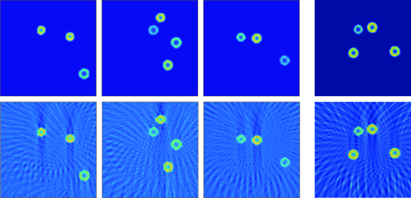
Figure 3: Training and evaluation data. Examples of randomly generated combinations of ring-shaped phantoms (top) and corresponding FBP reconstructions (bottom) containing under-sampling artifacts. The left three images contain examples from the training set; the right image is used for evaluation and is not part of the training data. In the FBP reconstructions one clearly sees the typical under-sampling artifacts.

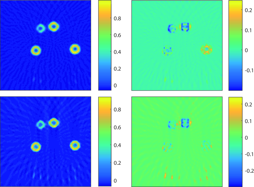
Figure 4: Results with the reconstruction networks. Top: Reconstructed image using the U-Net (left) and difference to the true phantom (right); the relative mean squared error is 0.026. Bottom: Reconstructed phantom using the S-net (left) and difference to the true phantom (right); the relative mean squared error is 0.33.

3.2 Network optimization

In order to optimize the reconstruction networks on the training data set $\mathcal{T}=\{(\mathbf{Y}_{n},\mathbf{X}_{n})\}_{n=1}^{N_{\mathcal{T}}}$, we use the mean absolute error as error metric in (6). This yields to the problem of finding the parameter vector $\mathcal{W}$ of the network function $\boldsymbol{\Phi}\triangleq\boldsymbol{\Phi}_{\mathcal{W}}$ by minimizing

$$E(\mathcal{T};\boldsymbol{\Phi}_{\mathcal{W}})\triangleq\sum_{n=1}^{N_{\mathcal{T}}}\lVert\mathbf{X}_{n}-\boldsymbol{\Phi}_{\mathcal{W}}(\mathbf{Y}_{n})\rVert_{1}\,.$$ (8)

For that purpose we did not use standard gradient descent, because evaluation of the full gradient is time consuming. Instead, we use stochastic batch gradient descent for minimizing (8). In batch stochastic gradient descent, at each sweep (a cycle of iterations), one partitions the training data into small random subsets of equal size (batch size) and then performs a gradient step with respect to each subset. To be precise, the update rule is given by

$$\mathcal{W}^{(k+1)}=\mathcal{W}^{(k)}-\eta\nabla_{\mathcal{W}}E(\mathcal{T}^{(k)},\boldsymbol{\Phi}_{\mathcal{W}^{(k)}})+\beta(\mathcal{W}^{(k)}-\mathcal{W}^{(k-1)})\,,$$ (9)

where $\mathcal{T}^{(k)}\subseteq\mathcal{T}$ is the training batch of the $k$th iteration and $\eta$ is called learning rate and $\beta$ momentum. Still, the training procedure can be costly. We emphasize, however, that the optimization has to be performed only once and prior to the actual image reconstruction. After training, the weights $\mathcal{W}$ are fixed and can be used to evaluate the reconstruction network $\boldsymbol{\Phi}=\boldsymbol{\Phi}_{\mathcal{W}}$ on new PAT data. In the present study, to optimize our networks we use a batch size of 1 and take $\eta=0.001$ and $\beta=0.99$.

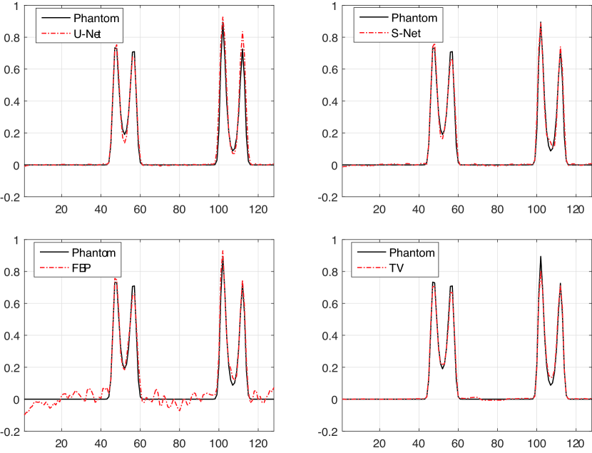
Figure 5: Horizontal cross sections. The images show horizontal cross section through the upper two rings comparing the original phantom with U-Net reconstruction (top left), the S-Net reconstruction (top right), the FBP reconstruction (bottom left) and the TV-minimization (bottom right).

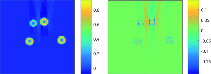
Figure 6: Results with TV-minimization. Reconstruction using TV-minimization (left) and difference to the true phantom (right). The relative mean squared error is 0.016.

3.3 Reconstruction results

Results with the reconstruction networks (the U-net and the S-net) are shown in Figure 4. We see that both networks are able to remove most of the under-sampling artifacts. The more complex U-Net gives better results, but also takes longer to train and apply. Taking a look at a horizontal cross section of the reconstructed phantom (Figure 5) we can see that both networks overestimate the minimal values within the ring structures. This suggests that classes of highly oscillating phantoms might be quite challenging to reconstruct. Further research is required to find out how to handle such cases. It is still surprising that the second NN, which is quite simple, performs that well. However, we expect that the S-net might struggle with more complex phantom classes. Anyway these results encourage to design new and well-suited networks for PAT image reconstruction.

For comparison purpose, we also tested TV minimization for image reconstruction,

$$\frac{1}{2}\lVert\mathds{A}(\mathbf{Y})-\mathbf{X}\rVert_{2}^{2}+\lambda\,\sum_{\mathbf{i}}\sqrt{\lvert(\mathds{D}_{1}\mathbf{X})_{\mathbf{i}}\rvert^{2}+\lvert(\mathds{D}_{2}\mathbf{X})_{\mathbf{i}}\rvert^{2}}\to\min_{\mathbf{X}}\,,$$ (10)

where $\mathds{D}=[\mathds{D}_{1},\mathds{D}_{2}]$ is the discrete gradient operator and $\lambda$ the regularization parameter. For solving (10) we use the algorithm proposed in [26] (an instance of the Pock-Chambolle algorithm [27] for TV minimization). Since the considered phantoms do not contain structures at different scales, TV-minimization method performs well, and in fact shows the lowest error relative mean squared error $\operatorname{MSE}(\mathbf{X})\triangleq\lVert\mathbf{X}-\mathbf{X}_{\rm rec}\rVert^{2}/\lVert\mathbf{X}\rVert_{2}^{2}$, where $\lVert\mathbf{X}\rVert_{2}$ denote the $\ell^{2}$-norm of $\mathbf{X}$. However, TV-minimization requires choosing a good regularization parameter and performing a relatively large number of iterations. For the results shown in Figure 6 we have chosen the optimization parameter $\lambda=0.005$ by hand and, in order to get small $\ell^{2}$-reconstruction error, performed 50 iterations. We note that the TV-minimization introduces new additional artifacts around the pair of rings which are relatively close together.

3.4 Computational resources

We used Keras [28] with TensorFlow [29] to train an evaluate the proposed reconstruction networks (U-Net and S-Net). The FBP and the TV-minimization are implemented in MATLAB. We ran all our experiments on a computer using an Intel i7-6850K and an NVIDIA 1080Ti. To iterate through our entire training set we need $5\text{\,}\mathrm{s}$ for the S-Net (7) and $16\text{\,}\mathrm{s}$ for the U-Net. Evaluating 100 sample images requires $0.9\text{\,}\mathrm{s}$ for the S-Net and $3.1\text{\,}\mathrm{s}$ for the U-Net. Hence a single image is reconstructed in a fraction of seconds by both methods; for example the S-net reconstructs the $128\times 128$ images at $111\text{\,}\mathrm{Hz}$ rate. One application with the current implementation of the discrete FBP takes $0.35\text{\,}\mathrm{s}$ and the used TV-minimization algorithm needs $0.94\text{\,}\mathrm{s}$ for one iteration. This results in an overall reconstruction time for TV minimization around $45\text{\,}\mathrm{s}$. Since the latter algorithms are implemented in MATLAB and do not use the GPU, the comparison of computation times is not completely fair and there is room for accelerating the FBP algorithm and TV-minimization. Especially, the FBP algorithm in combination with CNNs, both implemented on GPUs, will give high resolution artifact-free reconstructions in real time.

4 Conclusion

In this paper we proposed a deep learning framework for image reconstruction in PAT using sparse data including the limited view setting. The proposed reconstruction structure (5) consists in first applying the FBP algorithm and then using a CNN to remove artifacts. For the used CNN we investigated the established U-Net as well as the simple S-Net. Both of the proposed networks are able to improve the overall image quality. As expected, the more complex U-Net yields better result and offers a reconstruction quality comparable to iterative TV-minimization. Both reconstruction networks can be applied in real time, in contrast to iterative methods which are much slower. In future research, we will use more complex simulated and real-world PAT data, where we expect our method to be faster and comparable to TV-minimization in terms of reconstruction error. We also think it is beneficial to include adjustable weights in the backprojection step, which in the moment just used the FBP algorithms with prescribed weights.

References

- [1] Goodfellow, I., Bengio, Y., and Courville, A., [Deep Learning ], MIT Press (2016).
- [2] Antholzer, S., Haltmeier, M., and Schwab, J., “Deep learning for photoacoustic tomography from sparse data,” arXiv:1704.04587 (2017).
- [3] Chen, H., Zhang, Y., Zhang, W., Liao, P., Li, K., Zhou, J., and Wang, G., “Low-dose CT via convolutional neural network,” Biomed. Opt. Express 8(2), 679–694 (2017).
- [4] Kelly, B., Matthews, T. P., and Anastasio, M. A., “Deep learning-guided image reconstruction from incomplete data,” arXiv:1709.00584 (2017).
- [5] Han, Y., Yoo, J. J., and Ye, J. C., “Deep residual learning for compressed sensing CT reconstruction via persistent homology analysis,” (2016). http://arxiv.org/abs/1611.06391.
- [6] Jin, K. H., McCann, M. T., Froustey, E., and Unser, M., “Deep convolutional neural network for inverse problems in imaging,” IEEE Trans. Image Process. 26(9), 4509–4522 (2017).
- [7] Wang, G., “A perspective on deep imaging,” IEEE Access 4, 8914–8924 (2016).
- [8] Zhang, H., Li, L., Qiao, K., Wang, L., Yan, B., Li, L., and Hu, G., “Image prediction for limited-angle tomography via deep learning with convolutional neural network.” arXiv:1607.08707 (2016).
- [9] Ronneberge, O., Fischer, P., and Brox, T., “U-net: Convolutional networks for biomedical image segmentation,” CoRR (2015).
- [10] Reiter, A. and Bell, M. A. L., “A machine learning approach to identifying point source locations in photoacoustic data,” in [Proc. SPIE ], 10064, 100643J (2017).
- [11] Dreier, F., Haltmeier, M., and Pereverzyev, Jr., S., “Operator learning approach for the limited view problem in photoacoustic tomography.” arXiv:1705.02698 (2017).
- [12] Hauptmann, A., Lucka, F., Betcke, M., Huynh, N., Cox, B., Beard, P., Ourselin, S., and Arridge, S., “Model based learning for accelerated, limited-view 3d photoacoustic tomography,” arXiv:1708.09832 (2017).
- [13] Schwab, J., Antholzer, S., Nuster, R., and Haltmeier, M., “DALNet: High-resolution photoacoustic projection imaging using deep learning,” arXiv:1801.06693 (2018).
- [14] Kruger, R., Lui, P., Fang, Y., and Appledorn, R., “Photoacoustic ultrasound (PAUS) – reconstruction tomography,” Med. Phys. 22(10), 1605–1609 (1995).
- [15] Paltauf, G., Nuster, R., Haltmeier, M., and Burgholzer, P., “Photoacoustic tomography using a Mach-Zehnder interferometer as an acoustic line detector,” Appl. Opt. 46(16), 3352–3358 (2007).
- [16] Burgholzer, P., Bauer-Marschallinger, J., Grün, H., Haltmeier, M., and Paltauf, G., “Temporal back-projection algorithms for photoacoustic tomography with integrating line detectors,” Inverse Probl. 23(6), S65–S80 (2007).
- [17] Finch, D., Patch, S. K., and Rakesh, “Determining a function from its mean values over a family of spheres,” SIAM J. Math. Anal. 35(5), 1213–1240 (2004).
- [18] Haltmeier, M., “Inversion of circular means and the wave equation on convex planar domains,” Comput. Math. Appl. 65(7), 1025–1036 (2013).
- [19] Jaeger, M., Schüpbach, S., Gertsch, A., Kitz, M., and Frenz, M., “Fourier reconstruction in optoacoustic imaging using truncated regularized inverse k-space interpolation,” Inverse Probl. 23, S51–S63 (2007).
- [20] Kunyansky, L. A., “Explicit inversion formulae for the spherical mean Radon transform,” Inverse Probl. 23(1), 373–383 (2007).
- [21] Xu, M. and Wang, L. V., “Universal back-projection algorithm for photoacoustic computed tomography,” Phys. Rev. E 71(1), 016706 (2005).
- [22] Finch, D., Haltmeier, M., and Rakesh, “Inversion of spherical means and the wave equation in even dimensions,” SIAM J. Appl. Math. 68(2), 392–412 (2007).
- [23] Gratt, S., Nuster, R., Wurzinger, G., Bugl, M., and Paltauf, G., “64-line-sensor array: fast imaging system for photoacoustic tomography,” Proc. SPIE 8943, 894365 (2014).
- [24] Paltauf, G., Hartmair, P., Kovachev, G., and Nuster, R., “Piezoelectric line detector array for photoacoustic tomography,” Photoacoustics 8, 28–36 (2017).
- [25] Haltmeier, M., “Sampling conditions for the circular radon transform,” IEEE Trans. Image Process. 25(6), 2910–2919 (2016).
- [26] Sidky, E. Y., Jørgensen, J. H., and Pan, X., “Convex optimization problem prototyping for image reconstruction in computed tomography with the chambolle–pock algorithm,” Physics in medicine and biology 57(10), 3065 (2012).
- [27] Chambolle, A. and Pock, T., “A first-order primal-dual algorithm for convex problems with applications to imaging,” J. Math. Imaging Vision 40(1), 120–145 (2011).
- [28] Chollet, F. et al., “Keras.”, https://github.com/fchollet/keras, (2015).
- [29] Abadi, M., Agarwal, A., Barham, et al., “TensorFlow: Large-scale machine learning on heterogeneous systems,” (2015). Software available from tensorflow.org.