Effects of random pinning on the potential energy landscape of a supercooled liquid

Abstract

We use energy landscape methods to investigate the response of a supercooled liquid to random pinning. We classify the structural similarity of different energy minima, using a measure of overlap. This analysis reveals a correspondence between distinct particle packings (which are characterised via the overlap) and funnels on the energy landscape (which are characterised via disconnectivity graphs). As the number of pinned particles is increased, we find a crossover from a fluid state at low pinning to a glassy state at high pinning, in which all thermally accessible minima are structurally similar to each other. We discuss the consequences of these results for theories of randomly pinned liquids. We also investigate how the energy landscape depends on the fraction of pinned particles, including the degree of frustration and the evolution of distinct packings as the number of pinned particles is reduced.

I Introduction

A structural glass is a material that is mechanically solid but has an amorphous, liquid-like microstructure.BerthierB11 Glasses are normally produced by rapidly supercooling a liquid, which causes the constituent particles to move increasingly slowly until the system becomes solid on the experimental time scale. Several theories aim to describe this dynamical slowing down LubchenkoW07 ; ChandlerG10 ; gotzes88 by proposing that cooling the system brings it close to a critical point at which structural relaxation stops completely. This critical point might be thermodynamic in origin, adamg65 ; LubchenkoW07 or a purely dynamical effect, and the associated singularity might occur at some finite temperature, LubchenkoW07 ; gotzes88 or in a limit where the temperature tends to zero. ChandlerG10

Cammarota and Biroli CammarotaB11 proposed that by gradually pinning (immobilising) some of the particles in a supercooled liquid, one might observe a singularity at which structural relaxation of the remaining (unpinned) particles stops completely. This has been termed the random-pinning glass transition (RPGT). The associated singularity takes place at finite temperature, and shares many features with the singularity that occurs in random first-order transition (RFOT) theory. LubchenkoW07 In both the RPGT and RFOT transitions, slow (glassy) dynamics originates in a reduction of the entropy: a supercooled liquid may adopt many different amorphous structures, but a glass is a system that is localised on the observation time scale into a single metastable state, corresponding to a group of potential energy minima.

The theoretical proposal of Ref. CammarotaB11, has its roots in mean-field theory, and it is not clear whether these predictions are valid in physical (three-dimensional) fluids. Several numerical studies have investigated the effects of random pinning, ScheidlerKBP02 ; KimMS11 ; BerthierK12 ; KobB13 ; SzamelF13 ; FullertonJ14 ; OzawaKIM15 ; CammarotaS16 ; ChakrabartyDKD16 but have not yet established (or ruled out) the existence of an RPGT. Performing this test and accurately characterising the RPGT would require a comprehensive finite-size scaling analysis. However, the corresponding calculations converge slowly and the size-scaling approach is currently very expensive.

In this work, we use geometry optimisation methods Wales2003 to explore the potential energy landscape (PEL) of a randomly-pinned glassy fluid. Analysis of the PELs of glasses has a long history.Goldstein69 ; StillingerW82 ; StillingerW84 ; SastryDS98 ; SchroderSDG00 ; DoliwaH03 ; DoliwaH03b ; Heuer08 ; deSouzaW08 ; NiblettDSW16 A key advantage of using this approach to study the RPGT is that geometry optimisation methods such as basin-hopping (BH) global optimisationlis87 ; walesd97a and discrete path sampling (DPS)Wales02 ; Wales04 can treat activated relaxation events with arbitrarily high energy barriers. Exploring the accessible configuration space via DPS is efficient compared with conventional methods such as molecular dynamics that require waiting for many such events, which become increasingly rare as the glass transition is approached.

Our study combines energy landscape methods with an idea from mean-field theory, that a useful order parameter is the overlap $Q$, which measures the structural similarity of two configurations for a glassy system. FranzP97 ; MezardP99 We classify minima of the PEL according to their overlap, so that the RPGT (if it exists) is associated with localisation of the system, on long time scales, in a region of the landscape where all configurations are structurally similar (high-overlap). CammarotaB11 Our results are restricted to small systems ($N=256$ particles), but we do find a crossover on increasing the number of pinned particles, from low-overlap to high-overlap. These results are consistent with the predictions of Ref. CammarotaB11, , although the restriction to small systems means that we cannot distinguish whether the system has a smooth crossover from low- to high-overlap, or whether there might be a true phase transition.

In addition, we investigate how the PEL changes as particles are unpinned. We discuss the relationship between funnels on the energy landscape, the packing of the particles in space, and the overlap $Q$.

The structure of the paper is as follows: Sec. II describes our model and methods; and Sec. III characterises the crossover from low- to high-overlap, including a summary of the implications for the RPGT in Sec. III.8. Then Sec. IV analyses the varying degree of frustration of the landscape, following Ref. deSouzaSNFW17, . In Sec. V we analyse in more detail the dependence of the energy landscape on the number of pinned particles, by following the behaviour of distinct particle packings as the number of pinned particles is reduced. Finally, Sec. VI summarises our conclusions.

II Methods

II.1 Model

We consider a binary Lennard-Jones (BLJ) fluid. There are two atom types, larger A atoms and smaller B atoms, interacting via Lennard-Jones potentials with the popular Kob-Andersen parameter set.KobA95a This choice allows comparison with earlier numerical studies of the RPGT,BerthierK12 ; OzawaKIM15 ; ChakrabartyKD15 and with earlier work on the energy landscapes of glass-forming liquids.deSouzaW05 ; deSouzaW06 ; deSouzaW06b ; deSouzaW08 ; deSouzaW09 ; NiblettBWD17

The truncation of the interaction potential uses the Stoddard-Ford quadratic shifting scheme, StoddardF73 which ensures that the potential and its gradient are both continuous, as required for landscape analysis. Full details of the potential are given in Ref. deSouzaW05, : the truncation range is $r_{c}=2.5\,\sigma_{\rm AA}$. The system size is $N=256$ atoms, and we use a periodically-repeated cell with fixed number density 1.2$\,\sigma_{\rm AA}^{-3}$. $\mathbf{X}=(\bm{r}_{1},\bm{r}_{2},\dots,\bm{r}_{N})$ will denote a vector containing the positions of all particles.

Following convention, all lengths, energies, temperatures and times are given in reduced units, which can be expressed in terms of $\sigma_{\rm AA}$, $\epsilon_{\rm AA}$ and $m$, the mass of an A or B atom.

II.2 Pinning Particles

The random pinning method CammarotaB11 ; BerthierK12 ; OzawaKIM15 makes use of a reference configuration $\mathbf{X}^{*}$ that is sampled from the equilibrium (Boltzmann) distribution at some temperature $T_{0}$. Reference configurations were taken from molecular dynamics simulations, which were confirmed to be locally ergodic using the Mountain-Thirumalai fluctuation metric.ThirumalaiMK89 ; ThirumalaiM93 ; deSouzaW05

Let $c$ be the fraction of pinned particles, which means that $M=\left\lfloor{cN}\right\rfloor$ particles are chosen independently at random. The notation $\lfloor x\rfloor$ indicates the largest integer that is less than or equal to $x$. The positions of these $M$ particles are fixed, and one considers the energy of the system as a function of the position of the remaining (unpinned) particles. The potential energy surface (i.e. PEL) and associated Boltzmann distribution depend on $\mathbf{X}^{\ast}$ and on the set of pinned particles. Following the literature on spin glasses and other disordered systems, we refer to the combination of the reference configuration and the set of pinned particles as a realisation of the disorder. To obtain robust results one should average over many such realisations.

For each realisation of the disorder and each configuration $\mathbf{X}$ of the unpinned particles, the LBFGS algorithmNocedal80 ; LiuN89 was used to minimise the energy (always with the pinned particles fixed), so that each configuration can be associated to a local minimum of the PEL. The local minimum associated with the reference configuration $\mathbf{X}^{*}$ is the reference minimum $\mathbf{X}_{0}$.

All calculations performed in this paper, except those in sec. III.7, used reference temperature $T_{0}=0.5\,\epsilon_{\rm AA}/k_{\rm B}$. The results of Ozawa et al.OzawaKIM15 suggest that this should be the highest reference temperature at which the RPGT transition would be clearly observed for our model.

II.3 Comparing Structures: the overlap

Mean-field theory proposes that a useful order parameter in glassy systems is the overlap between two configurations $\mathbf{X}_{i},\mathbf{X}_{j}$. Several definitions are possible for the overlap,BiroliBCGV08 ; Berthier13 ; OzawaKIM15 ; DasCK17 and the general expectationBiroliC17 is that all definitions should lead to similar behaviour as long as two configurations have high overlap if and only if they are structurally similar. Following Ref. FullertonJ14, , our pinning procedure is independent of the particle types but the overlap depends only on the type-A particles:

$$Q(\mathbf{X}_{i},\mathbf{X}_{j})=\frac{1}{N_{m}}\sum_{k=1}^{N_{m}}\Theta(a-|\mathbf{r}_{k,i}-\mathbf{r}_{k,j}|).$$ (1)

Here, $k$ runs over the set of unpinned A-type atoms, and $N_{m}$ is the number of such atoms. $\Theta$ is the Heaviside step function, and $\mathbf{r}_{k,i}$ is the position vector of atom $k$ in configuration $\mathbf{X}_{i}$. Also, $a$ is a length scale parameter, which we set to $0.3\,\sigma_{\rm AA}$ following earlier work.OzawaKIM15 ; KobC14 ; Berthier13 Before calculating the overlap, permutational alignment is performed for $\mathbf{X}_{i}$ and $\mathbf{X}_{j}$ to account for indistinguishability of the mobile A atoms, using a shortest augmenting path algorithm.JonkerV87 ; WalesC12 This ensures that (for example) swapping the positions of two particles does not affect the overlap.

If $\mathbf{X}_{i}$ and $\mathbf{X}_{j}$ are very similar then $Q(\mathbf{X}_{i},\mathbf{X}_{j})\approx 1$, which is the largest possible value. The smallest possible value is $Q=0$, and independent random configurations typically have small values $Q\approx 0$. Based on the decay of overlap that happens during $\beta$-relaxation, BerthierBBKMR07 and on other previous work, BerthierJ15 ; OzawaKIM15 we introduce a threshold parameter $Q^{*}=0.7$ such that if $Q(\mathbf{X}_{i},\mathbf{X}_{j})>Q^{*}$ then we identify $\mathbf{X}_{i}$ and $\mathbf{X}_{j}$ as being structurally similar.

The overlap of an arbitrary configuration $\mathbf{X}$ with the reference minimum $\mathbf{X}_{0}$ is

$$Q_{0}(\mathbf{X})=Q(\mathbf{X},\mathbf{X}_{0}).$$ (2)

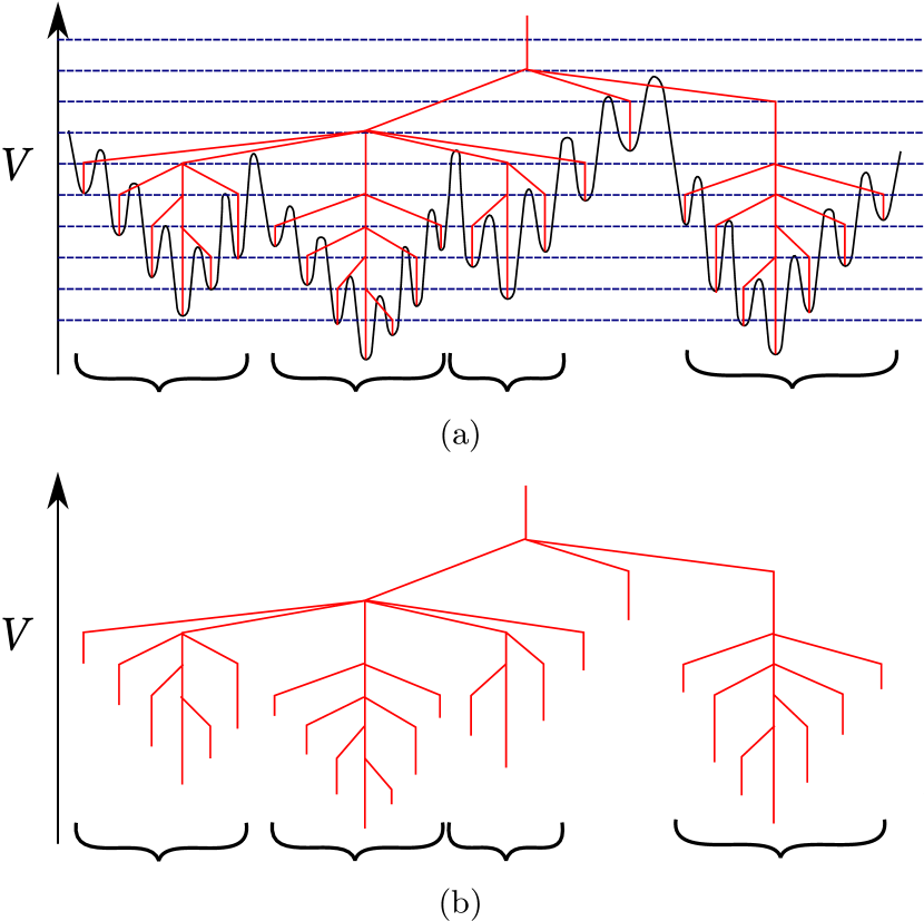
Figure 1: Top: Cartoon glassy PEL (in black) showing the disconnectivity graph construction (in red). Dashed blue lines indicate energy thresholds, brackets show the approximate extent of local funnels. Bottom: the disconnectivity graph that results from this cartoon landscape.

II.4 Potential Energy Landscape Methodology

The PEL of a pinned system is given by $V(\mathbf{X})$, which is a 3 $N_{m}$-dimensional function because the positions of the pinned atoms are constant. In the following we adapt standard geometry optimisation methods to identify local minima of $V(\mathbf{X})$, which control the thermodynamics at low temperatures, and transition states (stationary points with Hessian index one) which control the dynamics.

We classify minima of the pinned landscape according to their energies $V$ and their overlaps $Q_{0}$ with the reference minimum. We define a potential energy density of minima $g_{\rm IS}$ such that $g_{\rm IS}(V,Q_{0})\,dV\,dQ$ is the number of minima with energies between $V$ and $V+dV$ and overlaps between $Q_{0}$ and $Q_{0}+dQ$. We can also define a landscape entropy, $S_{\rm IS}(V)=k_{\text{B}}\ln g_{\rm IS}(V)$,SciortinoKT99 ; Wales2003 where $g_{\rm IS}(V)\,dV$ is the number of minima with energies between $V$ and $V+dV$. The subscript IS refers to “inherent structures”, an alternative nomenclature for PEL local minima.StillingerW82

II.4.1 Exploring the PEL: Identifying Minima

To locate minima of the PEL, we use the basin-hoppinglis87 ; walesd97a and basin-hopping parallel temperingStrodelLWW10 methods. The basin-hopping algorithm begins from a local minimum (see secs. III.1 and III.2 for different approaches to choosing the initial minimum). In each step, a new local minimum is proposed by perturbing the structure and performing local energy minimisation. The step is accepted or rejected using a Metropolis criterion with effective temperature $T_{\rm BH}$. If the step is accepted, the original minimum is stored in a database and the next step begins from the new minimum. Otherwise, the algorithm returns to the original minimum for the next step.

The two main parameters in this procedure are the maximum size of the structural perturbation, and the effective temperature $T_{\rm BH}$. These parameters control the rates at which new minima are discovered and accepted, respectively, but the true PEL being sampled is independent of both. The parameters are usually selected through trial and error to achieve a target acceptance rate for new minima, and may be varied dynamically during the calculation to assist this objective.

Basin-hopping locates low-energy minima efficiently, because the energy minimisation step removes downhill potential energy barriers between adjacent local minima. However, when a PEL contains many funnels (see below) the algorithm may become temporarily trapped in a single low-energy region and not explore alternative competing structures. Using a low $T_{\rm BH}$ exacerbates this problem, but using a high $T_{\rm BH}$ means that the low-energy regions may not be sampled adequately.

To avoid this problem, basin-hopping parallel tempering (BHPT) can be applied.StrodelLWW10 In BHPT, one considers $N_{r}$ replicas of the basin-hopping algorithm, each with a different value of $T_{\rm BH}$. By exchanging different configurations between the replicas, high-energy regions of the landscape may be crossed more efficiently.

Basin-hopping and BHPT both explore local minima efficiently, and can (in principle) be used to identify all minima on a PEL. Our strategy here is to generate a histogram of minimum energies and overlaps, which we denote by $\rho_{\rm IS}(V,Q_{0})$. In the limit where the algorithm samples the PEL exhaustively for a given range of $V$ and $Q_{0}$

$$\rho_{\rm IS}(V,Q_{0})\to g_{\rm IS}(V,Q_{0}).$$ (3)

In practice, the landscape is not explored exhaustively so there are systematic differences between $\rho_{\rm IS}$ and $g_{\rm IS}$, but we expect the important qualitative features of $g_{\rm IS}$ to be mirrored by $\rho_{\rm IS}$. This point is discussed in more detail during the analysis of the results.

II.4.2 Transition State Searches

Many properties of physical systems can be predicted by considering the statistics of local minima on the PEL, together with the transition states that connect them. To obtain information about transition states, we start from a database of minima and use double-ended searches, which take two local minima as input and identify a discrete path between them. A discrete path is a sequence of transition states and intermediate minima connected by steepest-descent paths.Wales02 ; Wales04 . Specifically, the doubly-nudgedTrygubenkoW04 ; SheppardTH08 elastic bandHenkelmanUJ00 ; HenkelmanJ00 (DNEB) algorithm is used to construct an approximate minimum energy pathway between pairs of minima. Structures corresponding to the local maxima on this pathway are candidate transition states, which are refined accurately using hybrid eigenvector-following (HEF).munrow99 ; Wales2003 ; ZengXH14 If a complete pathway between the original pair of minima has not been identified after one DNEB/HEF cycle, the Dijkstra algorithmDijkstra59 is used with a suitable distance metricCarrTW05 to select another pair of minima and another cycle is attempted. This procedure is repeated until the original pair of minima have been connected. Double-ended searches often add intermediate minima to the database as well as the connecting transition states.

Once transition states are known, energy barriers between minima may be measured. The overall barrier height from minimum $A$ to $B$ is defined as the energy difference between $A$ and the highest transition state on the minimum-energy pathway from $A$ to $B$.

II.4.3 Disconnectivity Graphs

After many transition state searches, one obtains a database of energy minima connected by transition states. To analyse the landscape, it is useful to generate a disconnectivity graph,BeckerK97 ; Wales2003 which can be interpreted by visual inspection. In these graphs, energy minima are represented as points, whose heights indicate the corresponding potential energy. These points are connected (upwards) to branching points: the energy of a branching point is (close to) the energy of the transition state that connects the minima below it. Transition state energies are rounded up to discrete energy levels to produce a clear visual representation. The process of generating a disconnectivity graph from a model glassy landscape is shown schematically in fig. 1.

Disconnectivity graphsBeckerK97 ; Wales2003 faithfully represent the energies of the local minima and the energy barriers between them, as determined from the transition states.

II.5 Landscape features: Funnels, metabasins, packings, and the configurational entropy

A central motivation for random pinning studies CammarotaB11 ; KobB13 is that they enable (in principle) the accessible configuration space of a system to be varied, without changing the temperature or the liquid structure, and hence without requiring extensive equilibration at low temperatures. Within mean-field theory, this effect is controlled by the configurational entropy, which measures the equilibrium occupation probabilities of metastable states. (Note that this quantity is not an experimental observable, and must be distinguished from the configurational part of the total entropy, which is defined in terms of the potential energy density of states.Wales2003 ) Within mean-field theory, the configurational entropy vanishes continuously at some finite pinning fraction $c=c^{*}$; this is the RPGT.

By investigating how the PEL changes with pinning, we can test how this mean-field prediction plays out in the pinned BLJ liquid. However, while the configurational entropy is a well-defined quantity in mean-field models, it does not have a unique definition in finite-dimensional systems where interactions have finite range, since metastable states have finite lifetimes in this case. Nevertheless, metastable states can be identified as regions of configuration space within which the system remains (dynamically) localised over sufficiently long time periods. See Ref. BiroliK01, for a discussion of how this construction can be applied consistently in both finite-dimensional and mean-field systems.

We consider three ways of identifying candidates for such states. We claim in the following that all these definitions identify a similar set of candidate metastable states.

A local funnel on the PEL is a group of minima for which barriers to reach a lower-energy minimum (downhill barriers) are systematically smaller than barriers to reach a higher-energy minimum (uphill barriers). Funnels are usually identified informally by visual inspection of disconnectivity graphs (see Fig. 1). Glassy landscapes typically contain many local funnels in the same energy range. Energy barriers between funnels are typically larger than barriers within funnels.

A metabasin is a group of minima between which dynamical transitions are rapid and easily reversible.DoliwaH03 ; DoliwaH03b Transitions between states in different metabasins are slower and should correspond to structural relaxation of the glass-former. In this sense, metabasins are similar to metastable states (albeit with finite lifetimes). Local funnels often correspond to metabasins.deSouzaW08

A packing of the particles is a group of minima with high mutual overlap and low overlap with other packings. Within mean-field theories, this method can be used to identify metastable states, but we emphasise that their definition does not include any dynamical information.

With these definitions in hand, we can define a measure of entropy that corresponds to the configurational entropy defined within mean-field theory. Suppose that for low temperatures $T$ the thermally-accessible configuration space for pinning fraction $c$ can be broken up into a set $\Lambda(c,T)$ of distinct packings, and that the canonical (Boltzmann) equilibrium occupation probability for packing $i$ is $p_{i}(c,T)$. Then a metastable state entropy, $S_{\rm MS}$, can be defined as

$$S_{\rm MS}(c,T)=-\sum_{i\in\Lambda(c,T)}p_{i}(c,T)\log p_{i}(c,T)$$ (4)

which depends implicitly on the system size $N$. To the extent that funnels and metabasins coincide with packings, the sum in (4) can be replaced by a sum over metabasins or funnels. On taking the thermodynamic limit, $S_{\rm MS}$ per particle is

$$s_{\rm MS}(c,T)=\lim_{N\to\infty}\frac{S_{\rm MS}(c,T)}{N}.$$ (5)

The mean-field prediction is that $s_{\rm MS}(c,T)$ vanishes continuously at the RPGT ($c=c^{*}$). Hence, for $c<c^{\ast}$ mean-field theory predicts $s_{\rm MS}>0$ but for $c>c^{\ast}$ then $s_{c}=0$. Recalling (4), this result means that for finite systems and $c>c^{\ast}$, the number of metastable states with significant occupation probabilities is sub-exponential in $N$: we will typically find that a single metastable state becomes dominant.

These hypotheses will be tested in the next Section. We do not attempt to measure $s_{\rm MS}$ directly, but we do find that for small $c$ then many packings contribute to the sum in (4), while for large $c$ then only a single packing contributes. These results show how the PEL evolves during this process, complementing previous studiesKobB13 ; OzawaKIM15 , which observed a dramatic decrease in the entropy of a supercooled liquid on increasing the pinning fraction $c$ through a critical value $c^{\ast}$.

We note that $S_{\rm MS}$ has similarities with several other measures of entropy. The landscape entropy $S_{\rm IS}$ is defined in a microcanonical framework in terms of the potential energy density of minima.SciortinoKT99 ; Wales2003 This landscape entropy can be estimated as the difference between the total entropy of the system and its vibrational entropy.SciortinoKT99 $S_{\rm IS}$ is not the same as $S_{\rm MS}$ because a metastable state does not correspond to a single energy minimum: the waiting time within minima is often quite short,Cavagna09 and $S_{\rm IS}$ is not expected to vanish at the RPGT. Other measures of metastable state entropy include the free energy cost required to localise the system in a state of high-overlap,BerthierC14 and direct counting of structural motifsKurchanL11 – our expectation is that these quantities should behave in a similar way to $S_{\rm MS}$.

III Results: Potential Energy Minima and Landscape Organisation

III.1 Return Times

To illustrate that increasing $c$ dramatically reduces the number of states with significant equilibrium occupation probability, we used basin-hopping to explore low-energy minima on the landscapes corresponding to several different pinning fractions. The reference minimum $\mathbf{X}_{0}$ has a low energy, and we expect it to be part of an accessible state for all $c$.

Let $\mathbf{X}(s)$ be the PEL minimum obtained after $s$ basin hopping steps, and let $Q_{0}(s)=Q(\mathbf{X}_{0},\mathbf{X}(s))$ be the overlap of this minimum with the reference minimum. We extracted the initial minima $\mathbf{X}(0)$ from molecular dynamics simulations of the pinned system with very high temperatures, so that $Q_{0}(0)$ would be small. 30 basin-hopping calculations were performed for each value of $c$, each with a structurally distinct initial minimum.

If the only accessible metastable state is the one containing the reference minimum, then we expect each basin-hopping calculation to converge to that state: $Q_{0}(s)>Q^{\ast}$ for large $s$. On the other hand, if there are many accessible states, one expects the algorithm to explore regions that are different from the reference configuration, so that $Q_{0}(s)$ will remain small.

Fig. 2 shows results for a single reference configuration ($T_{0}=0.5$) and various pinning fractions. We used an initial temperature parameter $T_{\rm BH}=5$, which was adjusted during the sampling to maintain an acceptance rate of 70%. Other parameter sets were found to give similar results, but the calculations were less efficient.

Fig. 2 shows that calculations with $c\geq 0.15$ tend to a large-$s$ limit of $\overline{Q}_{0}(s)>0.7$, indicating that the system approaches the reference minimum. For $c\leq 0.13$ we find $\overline{Q}_{0}(s)\lesssim 0.4$ for all $s$, indicating that the system is exploring a larger region of configuration space. These observations suggest a rather sharp crossover in the overlap as $c$ is increased, consistent with the predictions of Ref. CammarotaB11, .

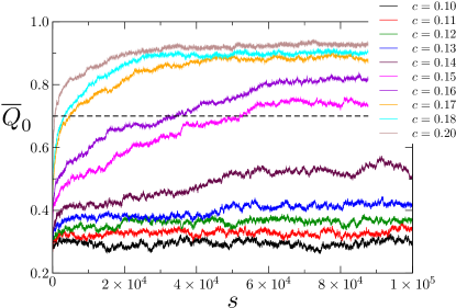
Figure 2: Plots showing how basin-hopping calculations explore overlap space at several different pinning fractions. $s$ denotes the number of basin-hopping steps taken, and $\overline{Q}_{0}(s)$ is the average of the overlap $Q_{0}$ for 30 basin-hopping runs with independent starting points. The dashed horizontal line shows $Q_{0}=Q^{\ast}$, which is the threshold used to define when structures are similar to the reference.

III.2 Distribution of Local Minima

To explore this crossover in more detail, we used basin-hopping parallel tempering (BHPT) to explore and sample the local minima of pinned BLJ, using the same reference configuration prepared at $T_{0}=0.5$. The aim is to estimate the density of minima $g_{\rm IS}(V,Q_{0})$, so the basin-hopping temperatures of the different replicas were selected to promote exploration of a large variety of minima. We found that for $T_{\rm BH}\gtrsim 25$ the range of minimum energies explored becomes constant, and replicas with $T_{\rm BH}<0.5$ do not explore new minima efficiently. Therefore, we used 12 basin-hopping replicas with $T_{\rm BH}$ spaced geometrically between $0.5$ and $25.0$, to allow efficient exchange of configurations between replicas. For each replica, 10 basin-hopping runs of $10^{5}$ steps were performed, and the results combined to produce a larger database of minima. The basin-hopping step size was varied dynamically to ensure that approximately 70% of steps located a new minimum.

Every basin-hopping replica was initialised at the reference minimum $\mathbf{X}_{0}$. This choice may bias the sampled distribution of minima towards high-$Q_{0}$ regions of the landscape, however the inclusion of high-temperature replicas which rapidly decorrelate from the initial minimum should limit this effect.

Fig. 3 shows contour plots of $\log_{10}\rho_{\rm IS}(V,Q_{0})$ for several values of $c$. The essential feature is that for $c\geq 0.17$ then all low-energy minima have $Q_{0}>0.7$, while for $c\leq 0.16$ there is significant density of states at low energy with $Q_{0}<0.7$, indicating that multiple metastable states are accessible. As in Fig. 2, this crossover occurs over a rather narrow range of $c$: the difference between $c=0.16$ and $c=0.17$ corresponds to pinning 3 extra atoms.

Recall from eq. (3) that the sampled distributions $\rho_{\rm IS}$ in Fig. 3 cannot be interpreted as direct measurements of $g_{\rm IS}$; these quantities coincide only in the limit of exhaustive sampling. However, we expect that regions where $\rho_{\rm IS}(V,Q_{0})=0$ probably have $g_{\rm IS}(V,Q_{0})\approx 0$, because there are relatively few minima at low energies and our results are consistent with having sampled almost all of them.

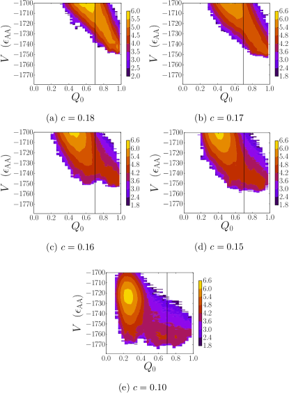
Figure 3: Contour plot of $\log_{10}\rho_{\rm IS}(V,Q_{0})$ for databases produced using BHPT. $\rho_{\rm IS}(V,Q_{0})$ is proportional to the number of minima in the database that have potential energy $V$ and overlap $Q_{0}$ with the reference minimum.

III.3 Global Probability of States

So far, all results have been shown for a single reference configuration. We have repeated our analysis for two other reference configurations, and five realisations of the disorder for each $\mathbf{X}^{\ast}$. To study the changing landscape as a function of $c$, we use consistent sequences of disorder realisations where the set of pinned atoms at each $c$ is a subset of the pinned atoms at all higher pinning fractions.

To summarise the results, we define

$$P(Q_{0}>0.7)=\int^{V_{c}}_{-\infty}\int_{0.7}^{1}\rho_{\rm IS}(V,Q_{0})~{}\text{d}Q_{0}\,\text{d}V,$$ (6)

where $V_{c}$ is an energy cutoff that restricts the integral to low energy (accessible) minima.

Fig. 4 shows $P(Q_{0}>0.7)$ as a function of $c$ for several sequences of disorder realisations, and the disorder average of this probability. For each sequence, one observes a crossover as $c$ is varied. The position and slope of the crossover vary between realisations, but the behaviour is similar in all cases, and the average probability also shows a crossover between $c\approx 0.14$ and $c\approx 0.17$.

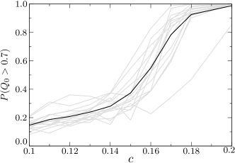
Figure 4: Probability that a low-energy minimum selected at random will be similar to the reference minimum. 15 realisations of the disorder are represented, indicated by grey lines. The black line represents the average value. Three different reference configurations were used, and the variation in $P(Q_{0}>0.7)$ between different disorder realisations with the same reference configuration is similar to the variation between different references.

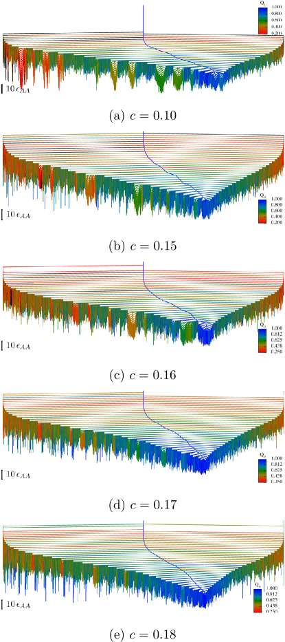
Figure 5: Disconnectivity graphs for landscapes generated by discrete path sampling between minima found in BHPT calculations. Minima are coloured by their value of $Q_{0}$.

III.4 Transition states

The results so far show that the distribution of local energy minima changes dramatically under random particle pinning. However, this analysis considers only the energies of the minima and their overlap $Q_{0}$ with the reference minimum. By projecting the landscape onto these coordinates, one discards a large amount of information, particularly the energies of the transition states (saddle points) that connect the minima. There may be multiple funnels/states where minima with similar $Q_{0}$ are separated by large barriers, which are not apparent from distributions such as $\rho_{\rm IS}(V,Q_{0})$. To resolve this detail, we consider the connectivity of the landscape.

We performed independent transition state sampling for each landscape depicted in fig. 3. Initially, 101 local minima were selected from each database. The reference minimum was always selected, and 100 other low-energy minima were chosen from a uniform distribution in $Q_{0}$. We then used the methods described in Sec. II.4.2 to calculate discrete paths between each pair of minima in the set of 101, a total of 5050 pairs. Combining the paths yielded a larger database of PEL minima and saddle points in the region of configuration space spanned by the initial set of 101 minima. Both low- and high-$Q_{0}$ regions of space were included.

III.5 Disconnectivity graphs

The landscape databases are represented in fig. 5 as disconnectivity graphs (see Sec. II.4.3). Each branch is coloured according to its overlap $Q_{0}$ with the reference minimum. The landscape corresponding to $c=0.10$ resembles an unpinned glassy PEL. In particular, it has many local funnels, which we have previouslydeSouzaW08 identified with metabasins.DoliwaH03 ; DoliwaH03b There is no dominant lowest-energy region of the PEL, but instead many of the local funnels have comparable energy.

At high pinning the PEL has a very different structure. In fig. 6(e) there is a single low-energy region of the PEL, which contains only minima similar to the reference minimum. That is, pinning $18\%$ of the particles has little effect on the landscape funnel that contains the reference state, but it acts to suppress other funnels. Single-funnelled landscapes usually correspond to structure-seeking systems,Wales12 which relax efficiently to their global minimum. In fig. 6(e), the main funnel contains quite high energy barriers and many minima with comparable energies, so reproducible relaxation to the global minimum is unlikely. However, the overall funnel structure means that relaxation to the region of minima with $Q_{0}>0.7$ will be fast and irreversible, except at very high temperatures. The result of pinning this many particles is that the landscape no longer resembles that of a structural glass former. We note, however, that this single-funnelled landscape includes minima with a wide range of $Q_{0}$, including low overlaps $Q_{0}\approx 0.2$. One should not imagine that pinning destroys all minima with low overlap. Rather, one finds that such minima still exist, but their energies are large, compared to the reference.

We also recall that Fig. 3 shows a significant difference between $c=0.16$ and $c=0.17$, where the possibility of minima with low energy and $Q_{0}<0.7$ disappears rather suddenly. The disconnectivity graphs in Fig. 5 indicate a smoother crossover as $c$ is varied: the low-overlap funnels that compete with the reference funnel at $c=0.16$ do not disappear on increasing to $c=0.17$; instead it seems that the energy of these funnels increases, so that they are no longer competitive with the reference funnel. We return to this point in Sec. V, below.

As a final comment on Fig. 5, note that there are a considerable number of minima with low energy and high $Q_{0}$, which nevertheless appear to be separated by large barriers from the reference funnel. This is probably due to “artificial trapping”:StrodelWW07 it is likely that there exist low-energy transition states connecting these minima to the reference funnel, but they have not been sampled in our transition state search. However, it is also possible that there are some large barriers between low-energy minima with high overlap, caused by the immovable pinned atoms.

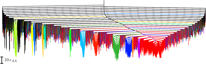
Figure 6: Disconnectivity graph for the database with $c=0.10$. Minima are assigned to packings using a greedy community detection algorithm, and each packing is coloured differently in the graph. Only packings containing more than 1000 minima are shown, all other minima are coloured black.

III.6 Packings on the PEL

In fig. 5 most local funnels are coloured uniformly, suggesting that the minima within each funnel are structurally similar. This similarity is expected in general for landscapes with funnels, particularly in glasses where the funnels are approximately equivalent to dynamical metabasins.deSouzaW08

To investigate the relationship between landscape structure and real-space structure, we use $Q$ as a similarity measure. In particular, we identify sets of minima, such that all minima within each set have a high mutual overlap $Q(\mathbf{X_{a}},\mathbf{X_{b}})$, while minima in different communities have low overlap. Physically, we argue that that these sets correspond to distinct packings of the particles, so that different minima within each packing typically differ by small local displacements. On the other hand, minima in different packings correspond to larger displacements, such as those that happen during structural relaxation of the liquid.

Many methods existWard63 ; GirvanN02 ; SzekelyR05 for detecting highly-connected sets in a graph with edge weights given by a similarity measure, but these typically require evaluation of all edge weights. Since our databases contain of order $10^{5}$ minima we use a greedy algorithm, which is typically much cheaper:

1. The “parent minimum”, $\mathbf{X}_{p}$, for the first packing is the reference minimum $\mathbf{X}_{0}$.

2. Compute $Q(\mathbf{X}_{p},\mathbf{X}_{m})$ for each minimum $\mathbf{X}_{m}$ not currently assigned to a packing.

3. If $Q(\mathbf{X}_{p},\mathbf{X}_{m})>Q^{\ast}$, add $m$ to the same packing as $p$.

4. Use the lowest-energy unassigned minimum as $\mathbf{X}_{p}$ for the next packing.

5. Iterate steps 2-4 until all unassigned minima lie above a predefined energy threshold.

The greedy algorithm does not guarantee that every minimum in a packing is more similar to the parent of that packing than to any other parent. However, it does guarantee that all minima within a packing are structurally close, and all parents are dissimilar to each other.

Fig. 6 shows the results of the greedy algorithm applied to a database at $c=0.10$. Branches are coloured according to the packing to which the corresponding minimum belongs. Most local funnels visible on the landscape correspond to a single packing, verifying that the the order parameter $Q$ can be used to detect whether two minima are in the same funnel. Of course, two configurations that are dissimilar from the reference minimum (small $Q_{0}$) might have a high mutual overlap (if they are in the same funnel) or a low mutual overlap, if they are in different funnels. In this sense the disconnectivity graph contains much more information than histograms such as Fig. 3, because it reveals the existence of multiple distinct packings/funnels.

However, we note that there are many minima in Fig. 6 that are identified as members of a packing, but are not members of any funnel. As in Fig. 5, this is likely a result of artificial kinetic trapping: these minima may be part of a funnel, but the relevant transition state has not been found.

III.7 Effect of Reference Temperature and System Size

So far all results have used reference configurations that are Boltzmann-distributed at $T_{0}=0.5$. Glassy features of the system are expected to become more accentuated on cooling, and mean-field theory predicts that $c^{\ast}$ decreases with $T_{0}$. To test these expectations, we used BHPT to sample energy minima with reference configurations obtained at $T_{0}=0.43$. Results for one reference configuration are shown in Fig. 7. Comparing with Fig. 3, we note that the high-overlap minima are separated in energy from the low-overlap ones for $c>0.13$, while this required a larger pinning fraction $c=0.17$ in Fig. 3. This effect is consistent with the theoretical picture of Ref. CammarotaB11, . Fig. 8 summarises the behaviour of five realisations of the disorder. As noted above, the crossover from low- to high-overlap occurs at a smaller value of $c$, compared with Fig. 4: this effect is consistent among different realisations of the disorder.

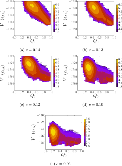
Figure 7: Density of states $\log_{10}\rho_{\rm IS}(V,Q_{0})$ for a sequence of disorder realisations with reference temperature $T_{0}=0.43\,\epsilon_{AA}/k_{\text{B}}$.

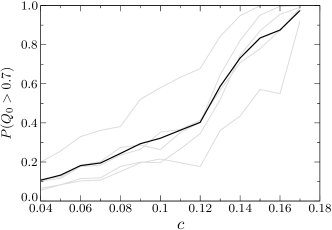
Figure 8: Probability that a low-energy minimum selected at random will be similar to the reference minimum, with reference temperature $T_{0}=0.43$. Five different reference configurations have been used. Grey lines indicate calculations from a single reference configuration, the black line is the disorder average.

The dependence of this crossover on $T_{0}$ and on system size is crucial for the theory of Ref. CammarotaB11, , which predicts a thermodynamic phase transition as $c$ is increased. Our results are not sufficient to investigate this prediction in detail, but Appendix A shows preliminary results for a smaller system ($N=180$ particles). The smaller systems show a clearer separation between high- and low-overlap, possibly because larger systems can support distinct high- and low-overlap regions within the same sample, making the crossover less sharp. The methods that we have introduced here provide a natural framework for investigating these questions.

III.8 Discussion

We summarise the conclusions so far. From Figs. 3 and 4, we see that increasing the number of pinned particles reduces the number of low-energy minima with significant equilibrium occupation probabilities. For $T_{0}=0.5$, there is a crossover at $c\approx 0.16$ so that for larger $c$, the accessible minima are mostly in the same packing as the reference minimum, as evidenced by their high overlap values $Q_{0}$. From Fig. 5, one sees that this crossover is accompanied by a change in the energy landscape, from a rough (glassy) landscape to a single-funnelled disconnectivity graph. From Figs. 5 and 6 one sees that the funnels observed in the disconnectivity graph are closely related to the packings that can be identified by analysis of the overlap (recall Sec. II.5). Figs. 7 and 8 show that lower reference temperatures make these effects more pronounced, particularly that there is a clearer distinction between high-overlap and low-overlap minima.

All these results are broadly consistent with the theoretical predictions of Ref. CammarotaB11, and with previous simulation work.KobB13 ; OzawaKIM15 The crossovers that we observe happen at slightly larger $c$ than predicted by Ref. OzawaKIM15, , and the effect of $T_{0}$ on the position of the crossover seems to be weaker. However, the quantities that we use to characterise this crossover are also quite different, so one does not expect quantitative agreement.

As noted above, understanding whether this crossover corresponds to a thermodynamic phase transition would require a more detailed analysis of different system sizes and temperatures. From a physical point of view, the first-order character of the RFOT transition predicts a clear separation between two sets of minima, that correspond to macrostates with high- and low-overlap. Intermediate values of the overlap should be strongly suppressed by the interfacial free energy cost associated with coexistence of different macrostates.KobB13 ; BerthierJ15 ; JackG16 Obtaining a clear separation between the minima with high- and low-overlap is hindered for $T_{0}=0.5$ because the relatively large number of pinned particles reduces the possibility of very small $Q_{0}$: it appears from Fig. 3 that the distributions for the (putative) high- and low-$Q$ macrostates are somewhat overlapping, and no clear trough is observed in the probability. One expects a clearer separation at lower $T_{0}$, where fewer particles are pinned, but this is not immediately apparent in Fig. 7. The absence of a clear separation between macrostates may be attributed to the relatively small system sizes used here: one expects that the distributions for the two macrostates should become narrower in larger systems, leading to a trough in the probability and (perhaps) to a directly-observable interface between high- and low-overlap states. Unfortunately, these larger systems are challenging numerically, as they are for other methods OzawaKIM15 ; KobB13 . For these reasons, we defer this question to later work.

In the remainder of this paper we discuss several other aspects of the energy landscapes in these pinned systems, particularly the degree of frustration, and the extent to which one can think of metabasins evolving smoothly on the landscape as $c$ is reduced.

IV Landscape frustration

In this section, we present quantitative descriptions of the change in landscape organisation as a function of $c$. First, we consider simple properties, which hint at the change in structure observed in fig. 5 and then we propose a more sophisticated metric to quantify this change directly.

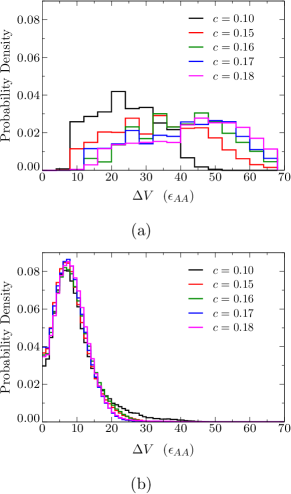
Figure 9: Histograms of the heights of energy barriers between local minima and the reference minimum. The first panel shows the “uphill” barriers, the second panel shows “downhill” barriers. The scale is the same for both panels.

Fig. 9 shows histograms of the energy barriers between local minima and the reference minimum for each landscape database. The barriers are divided into “uphill”, i.e. barriers to go from the reference minimum to a particular local minimum, and “downhill”, from the minimum to the reference.

The average uphill barrier increases systematically with $c$, because the sides of the main landscape funnel become steeper, as observed in fig. 5. In contrast, the mean downhill barrier is quite insensitive to $c$, but a long tail of high energy barriers develops as $c$ decreases. This tail corresponds to minima in low-energy funnels that have higher energy barriers to the reference than minima in the main funnel.

Fig. 9 and fig. 5 both indicate that pinned PELs become less frustrated as $c$ increases, meaning that there are fewer low-energy regions of the landscape separated by high barriers. Therefore the simulation time required to reach high-$Q_{0}$ minima will be small at high $c$.

Previously, we have characterised PELs using a frustration metric, $\widetilde{f}$, related to the efficiency of locating the global minimum from a randomly-chosen minimum.deSouzaSNFW17 In this case, we are interested in transition rates towards the PEL funnel that contains the reference minimum (which is not necessarily the global minimum). Therefore a modified frustration metric is used, based on the definition of packings presented in Sec. III.6:

$$\widetilde{f_{p}}=\sum_{\alpha\notin P_{0}}\widetilde{p}_{\alpha}^{\text{eq}}(T)\left(\frac{V_{\alpha}^{\dagger}-V_{0}}{\text{max}\{V_{\alpha}-V_{0},\Delta V\}}\right).$$ (7)

Here, $P_{0}$ is the the packing that contains the reference minimum, and $\alpha$ runs over all minima that do not belong to $P_{0}$. $p_{\alpha}^{\rm eq}(T)$ is the equilibrium occupation probability of $\alpha$, calculated within the harmonic superposition approximation.Wales93 ; Wales2003 $\widetilde{p}_{\alpha}^{\text{eq}}=p_{\alpha}^{\text{eq}}/(1-\sum_{\beta\in P_{0}}p_{\beta}^{\text{eq}})$ is the renormalised probability excluding all minima belonging to $P_{0}$. $V_{0}$ and $V_{\alpha}$ are the energies of the reference minimum and minimum $\alpha$, respectively.

$V_{\alpha}^{\dagger}$ is the energy of the highest transition state on the minimum-energy pathway connecting $\alpha$ to the reference, and $\Delta V=0.1\,\epsilon_{AA}$ is a parameter chosen to avoid divergence of $\widetilde{f_{p}}$ in cases where the reference minimum is not the global minimum.

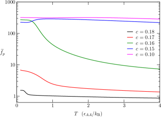
Figure 10: Modified frustration index $\widetilde{f_{p}}(T)$ for landscapes with different pinning fraction.

$\widetilde{f_{p}}$ is plotted in fig. 10 for the landscapes represented in fig. 5. Frustration decreases as a function of $c$ for the entire temperature range plotted, illustrating a major structural change in the PEL concurrent with the pinning transition. Over this range in $c$, the landscape transforms from a multifunnelled structure typical of supercooled liquids into a single-funnelled non-glassy structure. This result agrees with and reinforces our qualitative interpretation of fig. 5. The large range in $\widetilde{f_{p}}$ emphasises the magnitude of the change.

At low temperatures, $\widetilde{f_{p}}(T)$ varies more rapidly because the sum in eq. 7 is dominated by a few large terms. In particular, the frustration of the $c=0.16$ landscape increases dramatically, which may be a peculiarity of this particular disorder realisation, because several packings at $c=0.16$ are almost degenerate in energy with the reference minimum.

V Evolution of the PEL as the Pinning Fraction is reduced

In this section, we examine the effects of random pinning by following the behaviour of particular minima and packings as $c$ changes. For example, we consider the overlap between minima in landscapes that have different $c$, and hence appear in different panels of Fig. 5.

We perform this analysis by starting from a high-$c$ landscape ($c=c_{0}=0.18$), and unpinning atoms one by one (always in the same sequence), relaxing the PEL minima by energy minimisation after each atom is unpinned. New sets of minima at lower values of $c$ are obtained.

One might imagine a complementary procedure, following the evolution of minima as $c$ is increased. This approach would be interesting, but it is difficult to implement because there is no unique route to obtain a minimum at $c_{0}$, given an initial minimum at some lower pinning fraction $c$. We therefore leave this analysis for future work.

V.1 Evolution of the Minima

We studied the properties of a set of minima during unpinning from $c_{0}=0.18$. This set included the reference minimum at $c_{0}$, and the parent minimum of every packing that contained at least 1000 minima.

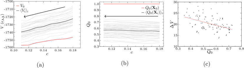
Figure 11: Figures showing how $V$ and $Q_{0}$ evolve for a set of minima with progressive unpinning from a $c=0.18$ landscape (as indicated by the arrows). Each grey line represents the parent minimum of a large packing on the $c=0.18$ landscape. The thick black line represents the average value over the grey lines. The red line represents the reference minimum. Panel (c) shows how the energy change during unpinning depends on the overlap of the minimum. $\Delta\,V$ is the energy difference between a minimum at $c=0.18$ and the corresponding minimum at $c=0.10$, $\overline{Q_{0}}$ is the average $Q_{0}$ of those two minima. The best-fit trend line is shown, which has correlation coefficient -0.463.

Fig. 11(a) shows how the energies of these minima change during unpinning. The energy of each minimum decreases, because the energy is reminimised after each particle is unpinned. For most minima this decrease is substantial: around $20\,\epsilon_{AA}$ on average. Because the reference minimum decreases by only $10\,\epsilon_{AA}$ over the same interval, this result means that the offset between the reference minimum and the other funnels decreases during unpinning. Fig. 11(b) shows little change in $Q_{0}$ during unpinning, indicating that most packings do not undergo significant structural change when pinned atoms are released.

V.2 Evolution of the Packings

We now consider the evolution of packings (groups of minima), as $c$ is decreased. We took a sample of 101 minima representing all the large packings at $c=c_{0}=0.18$, and used the unpinning procedure to obtain the corresponding minima at $c=0.17$. For both pinning fractions, we found discrete paths between every pair of minima, ensuring full connectivity. We also repeated this unpinning procedure to obtain databases at $c=0.16$ and $c=0.15$. Fig. 12 shows the disconnectivity graphs for $c=0.17$ and $c=0.16$.

We emphasise that the disconnectivity graph obtained by unpinning in fig. 12 is not at all equivalent to the graphs shown in fig. 5, even if the value of $c$ is the same. The set of minima used to initialise the path-sampling calculation in fig. 5 were obtained by BHPT sampling at the same value of $c$ as the transition states. In contrast, the minima used for path-sampling in fig. 12 were obtained by relaxing minima that were sampled by BHPT at a higher value of $c$. Therefore the disconnectivity graphs in fig. 12 may be thought of as the subset of the $c=0.17$ and $c=0.16$ landscapes that is directly related to minima that also exist on the $c=0.18$ landscape, whereas fig. 5 represents a sample of the entire PEL at each value of $c$.

Note the differences between the two figures: in the $c=0.16$ panel of fig. 5 there are several low-$Q_{0}$ packings with energies within 1-2 $\epsilon_{\rm AA}$ of the reference structure, but the gap in the $c=0.16$ panel of fig. 12 is significantly larger. Our methods do not allow us to follow minima as $c$ increases, but the natural conclusion here is that the packings that exist (for $c=0.16$) with low energy and low $Q_{0}$ are somehow “projected out” as the number of pinned particles is increased, which explains why they have no counterparts in the high-$c$ landscape. This is consistent with the theory of random pinning.CammarotaB11

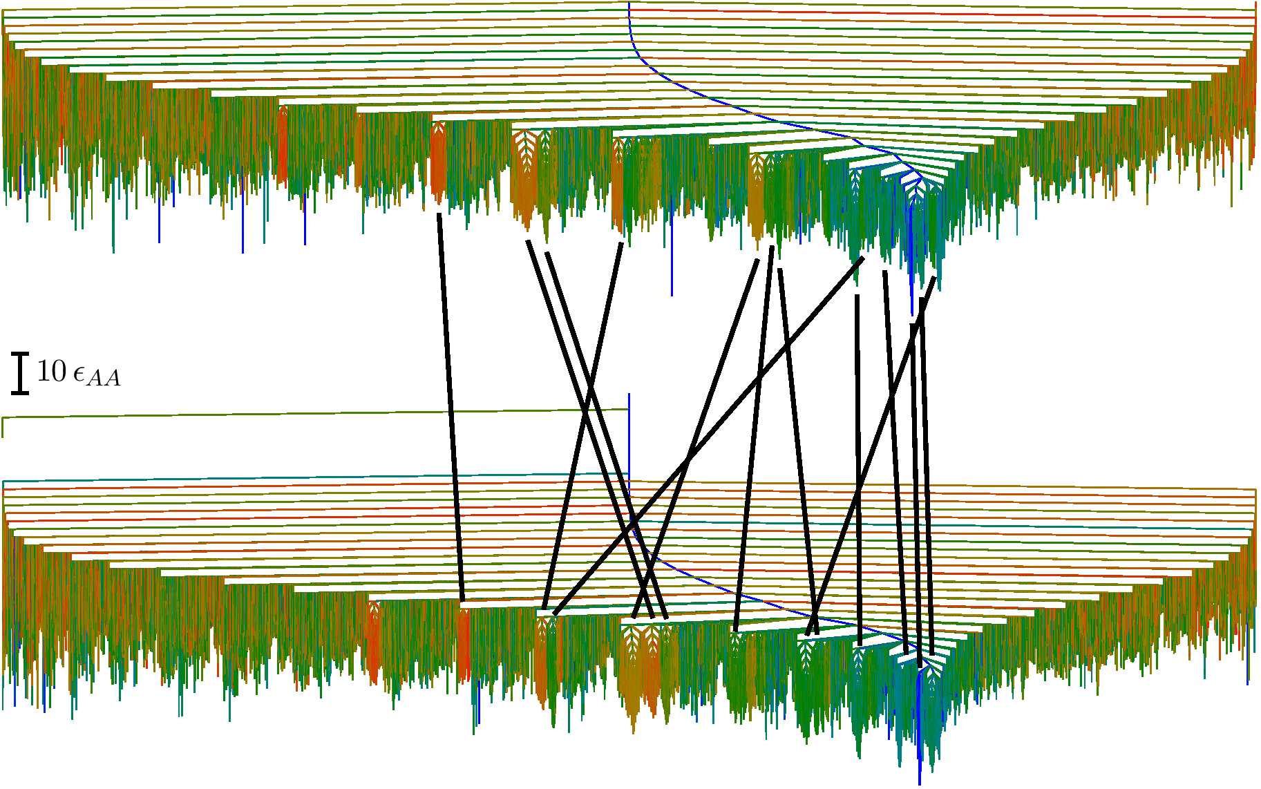
Figure 12: Top panel: correspondence between packings in different disconnectivity graphs. The upper graph represents a landscape with $c=0.17$, the lower graph is at $c=0.16$. Black lines connect some of the packings on the two landscapes that have $\mathcal{Q}>0.7$. Minima are coloured according to their $Q_{0}$ values, using the same colour scale as before.

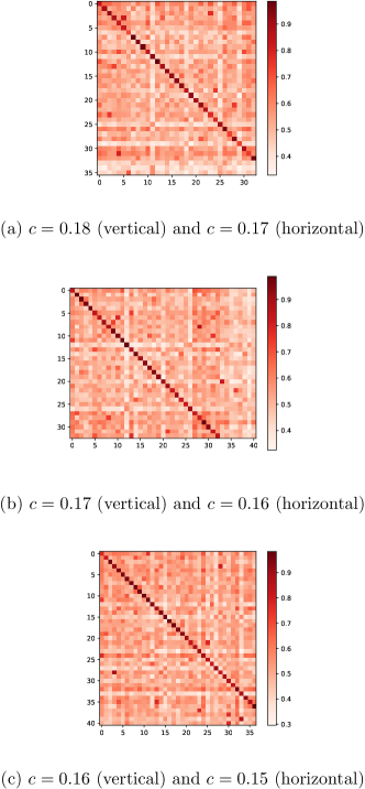
Figure 13: Heat maps of matrices representing the average overlap between low-lying minima in different packings for two landscapes with different $c$. Packings have been ordered to maximise overlap along the main diagonal.

We used the packing-detection algorithm of Sec III.6 to identify packings in both landscapes, restricting to packings that contain at least 1000 minima. We estimated the mutual overlap between pairs of packings: for two packings $A,B$ we define

$${\cal Q}(A,B)=\frac{1}{{\cal N}_{A}{\cal N}_{B}}\sum_{X\in A}\sum_{Y\in B}Q(X,Y)$$

where the sums run over all minima within each packing (the number of minima in packing $A$ is ${\cal N}_{A}$, etc). In practice, we estimate $\cal Q$ by selecting 10 minima at random from each packing. The sum in the overlap calculation includes all atoms that are unpinned in the lower-$c$ configuration.

Fig. 13 shows ${\cal Q}(A,B)$ for different pairs of landscapes. The labelling of the packings is arbitrary; they have been ordered using the Hungarian algorithmKuhn55 ; Munkres57 to maximise the overlap along the main diagonal of each panel. Most packings at the lower value of $c$ have high overlap with exactly one “parent packing” from the higher $c$. Some of the correspondences between parent and daughter packings are shown in Fig. 12. As in Fig. 11, one sees that packings retain their identities as $c$ is reduced, but fig. 12 also shows that the energy gap between the reference and low-$Q_{0}$ minima decreases slightly as $c$ is reduced. This observation indicates a weak negative relationship between $Q_{0}$ and the energy decrease during unpinning, which is illustrated by fig. 11(c).

As well as pairs of packings that have a clear parent-daughter relationship, there are several other scenarios that can (and do) occur. First, there may be packings on the low-$c$ landscape that have no apparent parent on the high-$c$ landscape. These features correspond to columns in Fig. 13 in which no large values appear. In this case, unpinning leads to new packings that were not present at higher $c$, consistent with an increasing value of $S_{\rm MS}$ as $c$ is reduced. Second, there may be packings on the high-$c$ landscape that have no clear daughter on the low-$c$ landscape – these correspond to rows in Fig. 13 with no large values. In this case, unpinning some atoms has presumably led to a significant rearrangement in the structure of the system – the original packing may have been stabilised by one of the pinned atoms, and is destroyed by unpinning. Third, there may be daughter packings (at low $c$) with more than one parent; and there may be parent packings (at high $c$) with more than one daughter. These correspond to splitting or merging of packings as $c$ is reduced. Fourth, we sometimes observe two parent and two daughter packings, such that both parents have high overlap with both daughters: in Fig. 13 one then sees an off-diagonal element with a large value of $\cal Q$, together with a large value of $\cal Q$ in the corresponding transposed element. This scenario indicates pairs of packings that are structurally similar, but not similar enough to be identified as a single packing by our packing-detection algorithm.

To end this section, recall that the original theoretical picture of random pinning CammarotaB11 is that $S_{\rm MS}$ is reduced as $c$ is increased, leading to an RPGT when there is only one packing with appreciable occupation probability. Here we have considered the unpinning process (decreasing $c$), which limits our ability to draw conclusions about the behaviour when $c$ increases. In particular, since the packings shown in Fig. 13 are obtained by successive unpinning, one tends not to sample low-$c$ packings that lack any “parent” (in the higher-$c$ landscape). To the extent that this limitation may be ignored, our results follow the qualitative behavior predicted by mean-field theory,CammarotaB11 although situations in which some packings have multiple parents or multiple daughters are not expected in mean-field models.

VI Conclusions

We have analysed the energy landscape of a randomly-pinned glassy fluid, using the overlap $Q$ as an order parameter. As the pinning fraction $c$ is increased, the energy landscape crosses over from a typical glassy structure with many funnels, into a single-funnelled structure in which all thermally-accessible minima have high overlap with the reference minimum. These observations match the situation anticipated by Cammarota and Biroli,CammarotaB11 although the data presented here cannot resolve whether this crossover corresponds to the predicted thermodynamic phase transition. We showed that the overlap, which is the natural order parameter within mean-field theories of the glass transition,FranzP97 ; MezardP99 can be used to define distinct packings of the particles, and that these packings can be identified with funnels on the energy landscape. We propose that packings represent physically relevant metastable states, such that the associated entropy $S_{\rm MS}$ should vanish at the RPGT. Future numerical work could test this hypothesis.

We quantified the change in landscape structure by calculating a frustration metric, which indicates that thermodynamic and dynamic bias towards the reference structure is greater at high $c$ than low $c$. In addition, we introduced methods for tracking packings (and individual minima), as $c$ is reduced. The results indicate a complex phenomenology, where packings typically seem to retain their identity as $c$ changes, but they can also split and merge.

The methodology presented here offers a new route for investigating the effects of random pinning in amorphous systems, providing a link between mean-field theories and the potential energy landscape.

Appendix A Effect of System Size

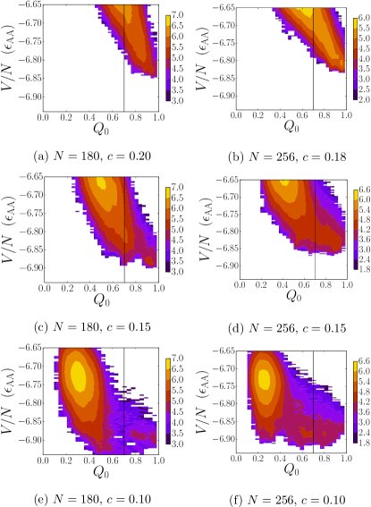
Figure 14: Histograms comparing $\rho_{\rm IS}(V,Q_{0})$ between different system sizes. All graphs have the same vertical scale.

If the RPGT is an equilibrium phase transition, $P(Q_{0}>0.7)$ should be discontinuous in the thermodynamic limit, because the number of distinct metastable states would change suddenly at $c^{\ast}$. Finite-size effects suppress this discontinuity,Yeomans1992 ; Goldenfeld1992 but can in principle be removed by system size scaling analysis. The gradient of $P(Q_{0}>0.7)$ at the crossover should extrapolate to infinity in the infinite system-size limit if the landscape transformation corresponds to a thermodynamic event. Also, in large systems, one expects to see a bimodal distribution $\rho_{\rm IS}(V,Q_{0})$, with two populations of minima (high- and low-overlap), that are separated by a deep trough in the probability. This trough represents the interfacial-free-energy cost to nucleate a configuration with low-overlap, within a high-overlap system.

As an initial step towards this scaling analysis, fig. 14 presents $\rho_{\rm IS}(V,Q_{0})$ for a smaller BLJ simulation cell containing 180 atoms (144 A-type and 36 B-type), and comparable plots for the 256-atom landscapes. No qualitative differences are observed between the two systems, which may indicate that the landscape properties we probe are broadly independent of system size. The density of minima with $Q_{0}$ values intermediate between the high- and low-overlap states (i.e. $Q_{0}\approx 0.7$) is slightly smaller in the smaller system. This result may suggest that the larger system is better able to support distinct high- and low-$Q_{0}$ regions within the same configuration, which tends to “smooth out” the sharp transition predicted in mean-field theory (or push it to lower temperature).

References

- (1) Berthier, L. and Biroli, G., Rev. Mod. Phys., 83, 587 (2011)
- (2) Lubchenko, V. and Wolynes, P.G., Ann. Rev. Phys. Chem., 58, 235 (2007)
- (3) Chandler, D. and Garrahan, J.P., Annual Review of Physical Chemistry, 61, 191 (2010)
- (4) Götze, W. and Sjögren, L., J. Phys. C., 21, 3407 (1988)
- (5) Adam, G. and Gibbs, J.H., J. Chem. Phys. , 43, 139 (1965)
- (6) Cammarota, C. and Biroli, G., Proc. Natl. Acad. Sci. USA, 109, 8850 (2012)
- (7) Scheidler, P., Kob, W., Binder, K. and Parisi, G., Philosophical Magazine B, 82, 283 (2002)
- (8) Kim, K., Miyazaki, K. and Saito, S., Journal of Physics: Condensed Matter, 23, 234123 (2011)
- (9) Berthier, L. and Kob, W., Physical Review E - Statistical, Nonlinear, and Soft Matter Physics, 85, 011102 (2012)
- (10) Kob, W. and Berthier, L., Phys. Rev. Lett., 110, 245702 (2013)
- (11) Szamel, G. and Flenner, E., Europhys. Lett., 101, 66005 (2013)
- (12) Fullerton, C.J. and Jack, R.L., Physical Review Letters, 112, 255701 (2014)
- (13) Ozawa, M., Kob, W., Ikeda, A. and Miyazaki, K., Proc. Natl. Acad. Sci. USA, 112, 6914 (2015)
- (14) Cammarota, C. and Seoane, B., Phys. Rev. B, 94, 180201 (2016)
- (15) Chakrabarty, S., Das, R., Karmakar, S. and Dasgupta, C., J. Chem. Phys., 145, 034507 (2016)
- (16) Wales, D.J., Energy Landscapes, (Cambridge University Press, Cambridge, 2003)
- (17) Goldstein, M., J. Chem. Phys. , 51, 3728 (1969)
- (18) Stillinger, F.H. and Weber, T.A., Phys. Rev. A, 25, 978 (1982)
- (19) Stillinger, F.H. and Weber, T.A., Science, 225, 983 (1984)
- (20) Sastry, S., Debenedetti, P.G. and Stillinger, F.H., Nature, 393, 554 (1998)
- (21) Schroder, T.B., Sastry, S., Dyre, J.C. and Glotzer, S.C., J. Chem. Phys., 112, 9834 (2000)
- (22) Doliwa, B. and Heuer, A., Phys. Rev. E, 67, 031506 (2003)
- (23) Doliwa, B. and Heuer, A., Phys. Rev. E, 67, 030501(R) (2003)
- (24) Heuer, A., J. Phys. Cond. Mat., 20, 373101 (2008)
- (25) de Souza, V.K. and Wales, D.J., J. Chem. Phys., 129, 164507 (2008)
- (26) Niblett, S.P., de Souza, V.K., Stevenson, J.D. and Wales, D.J., J. Chem. Phys., 145, 024505 (2016)
- (27) Li, Z. and Scheraga, H.A., Proc. Natl. Acad. Sci. USA, 84, 6611 (1987)
- (28) Wales, D.J. and Doye, J.P.K., J. Phys. Chem. A, 101, 5111 (1997)
- (29) Wales, D.J., Mol. Phys., 100, 3285 (2002)
- (30) Wales, D.J., Mol. Phys., 102, 891 (2004)
- (31) Franz, S. and Parisi, G., Phys. Rev. Lett. , 79, 2486 (1997)
- (32) Mézard, M. and Parisi, G., Phys. Rev. Lett., 82, 747 (1999)
- (33) De Souza, V.K., Stevenson, J.D., Niblett, S.P., Farrell, J.D. and Wales, D.J., J. Chem. Phys., 146, 124103 (2017)
- (34) Kob, W. and Andersen, H., Phys. Rev. E, 51, 4626 (1995)
- (35) Chakrabarty, S., Karmakar, S. and Dasgupta, C., Scientific Reports, 5, 12577 (2015)
- (36) de Souza, V.K. and Wales, D.J., J. Chem. Phys., 123, 134504 (2005)
- (37) de Souza, V.K. and Wales, D.J., Phys. Rev. B., 74, 134202 (2006)
- (38) de Souza, V.K. and Wales, D.J., Phys. Rev. Lett., 96, 057802 (2006)
- (39) de Souza, V.K. and Wales, D.J., J. Chem. Phys., 130, 194508 (2009)
- (40) Niblett, S.P., Biedermann, M., Wales, D.J. and de Souza, V.K., J. Chem. Phys. , 147, 152726 (2017)
- (41) Stoddard, S.D. and Ford, J., Phys. Rev. A, 8, 1504 (1973)
- (42) Thirumalai, D., Mountain, R.D. and Kirkpatrick, T.R., Phys. Rev. A, 39, 3563 (1989)
- (43) Thirumalai, D. and Mountain, R.D., Phys. Rev. E, 47, 479 (1993)
- (44) Nocedal, J., Math. Comput., 35, 773 (1980)
- (45) Liu, D. and Nocedal, J., Math. Prog., 45, 503 (1989)
- (46) Biroli, G., Bouchaud, J.P., Cavagna, A., Grigera, T.S. and Verrocchio, P., Nature Physics, 4, 771 (2008)
- (47) Berthier, L., Phys. Rev. E, 88, 022313 (2013)
- (48) Das, R., Chakrabarty, S. and Karmakar, S., Soft Matter, 13, 6929 (2017)
- (49) Biroli, G. and Cammarota, C., Phys. Rev. X, 7, 011011 (2017)
- (50) Kob, W. and Coslovich, D., Phys. Rev. E, 90, 052305 (2014)
- (51) Jonker, R. and Volgenant, A., Computing, 38, 325 (1987)
- (52) Wales, D.J. and Carr, J.M., Journal of Chemical Theory and Computation, 8, 5020 (2012)
- (53) Berthier, L., Biroli, G., Bouchaud, J.P., Kob, W., Miyazaki, K. and Reichman, D.R., The Journal of Chemical Physics, 126, 184503 (2007)
- (54) Berthier, L. and Jack, R.L., Phys. Rev. Lett., 114, 205701 (2015)
- (55) Sciortino, F., Kob, W. and Tartaglia, P., Phys. Rev. Lett. , 83, 3214 (1999)
- (56) Strodel, B., Lee, J.W.L., Whittleston, C.S. and Wales, D.J., Journal of the American Chemical Society, 132, 13300 (2010)
- (57) Trygubenko, S.A. and Wales, D.J., J. Chem. Phys., 120, 2082 (2004)
- (58) Sheppard, D., Terrell, R. and Henkelman, G., J. Chem. Phys. , 128, 134106 (2008)
- (59) Henkelman, G., Uberuaga, B.P. and Jónsson, H., J. Chem. Phys., 113, 9901 (2000)
- (60) Henkelman, G. and Jónsson, H., J. Chem. Phys., 113, 9978 (2000)
- (61) Munro, L.J. and Wales, D.J., Phys. Rev. B, 59, 3969 (1999)
- (62) Zeng, Y., Xiao, P. and Henkelman, G., J. Chem. Phys. , 140, 044115 (2014)
- (63) Dijkstra, E.W., Numerische Mathematik, 1, 269 (1959)
- (64) Carr, J.M., Trygubenko, S.A. and Wales, D.J., J. Chem. Phys., 122, 234903 (2005)
- (65) Becker, O.M. and Karplus, M., J. Chem. Phys., 106, 1495 (1997)
- (66) Biroli, G. and Kurchan, J., Phys. Rev. E, 64, 016101 (2001)
- (67) Cavagna, A., Phys. Rep., 476, 51 (2009)
- (68) Berthier, L. and Coslovich, D., Proc. Natl. Acad. Sci. USA, 111, 11668 (2014)
- (69) Kurchan, J. and Levine, D., J. Phys. A, 44, 035001 (2011)
- (70) Wales, D.J., Phil. Trans. Roy. Soc. A, 370, 2877 (2012)
- (71) Strodel, B., Whittleston, C.S. and Wales, D.J., J. Am. Chem. Soc., 129, 16005 (2007)
- (72) Ward, J.H., Journal of the American Statistical Association, 58, 236 (1963)
- (73) Girvan, M. and Newman, M.E.J., Proc. Natl. Acad. Sci. USA, 99, 7821 (2002)
- (74) Szekely, G.J. and Rizzo, M.L., Journal of Classification, 22, 151 (2005)
- (75) Jack, R.L. and Garrahan, J.P., Phys. Rev. Lett. , 116, 055702 (2016)
- (76) Wales, D.J., Molecular Physics, 78, 151 (1993)
- (77) Kuhn, H.W., Naval Research Logistics Quarterly, 2, 83 (1955)
- (78) Munkres, J., Journal of the Society for Industrial and Applied Mathematics, 5, 32 (1957)
- (79) Yeomans, J.M., Statistical Mechanics of Phase Transitions, (Clarendon Press, Oxford, 1992)
- (80) Goldenfeld, N., Lectures on Phase Transitions and the Renormalization Group, (Addison-Wesley, Reading, MA, 1992)