Resource-Aware Algorithms for
Distributed Loop Closure Detection
with Provable Performance Guarantees

Abstract

Inter-robot loop closure detection, e.g., for collaborative simultaneous localization and mapping (CSLAM), is a fundamental capability for many multirobot applications in GPS-denied regimes. In real-world scenarios, this is a resource-intensive process that involves exchanging observations and verifying potential matches. This poses severe challenges especially for small-size and low-cost robots with various operational and resource constraints that limit, e.g., energy consumption, communication bandwidth, and computation capacity. This paper presents resource-aware algorithms for distributed inter-robot loop closure detection. In particular, we seek to select a subset of potential inter-robot loop closures that maximizes a monotone submodular performance metric without exceeding computation and communication budgets. We demonstrate that this problem is in general NP-hard, and present efficient approximation algorithms with provable performance guarantees. A convex relaxation scheme is used to certify near-optimal performance of the proposed framework in real and synthetic SLAM benchmarks.

1 Introduction

Multirobot systems provide efficient and sustainable solutions to many large-scale missions. Inter-robot loop closure detection, e.g., for collaborative simultaneous localization and mapping (CSLAM), is a fundamental capability necessary for many such applications in GPS-denied environments. Discovering inter-robot loop closures requires (i) exchanging observations between rendezvousing robots, and (ii) collectively verifying potential matches. In many real-world scenarios, this is a resource-intensive process with a large search space due to, e.g., perceptual ambiguity, infrequent rendezvous, and long-term missions [4, 12, 15, 10]. This task becomes especially challenging for prevalent small-size and low-cost platforms that are subject to various operational or resource constraints such as limited battery, low-bandwidth communication, and limited computation capacity. It is thus crucial for such robots to be able to seamlessly adapt to such constraints and intelligently utilize available on-board resources. Such flexibility also enables robots to explore the underlying trade-off between resource consumption and performance, which ultimately can be exploited to save mission-critical resources. Typical ad hoc schemes and heuristics only offer partial remedies and often suffer from arbitrarily poor worst-case performance. This thus motivates the design of reliable resource-aware frameworks that provide performance guarantees.

This paper presents such a resource-aware framework for distributed inter-robot loop closure detection. More specifically, given budgets on computation (i.e., number of verification attempts) and communication (i.e., total amount of data transmission), we seek to select a budget-feasible subset of potential loop closures that maximizes a monotone submodular performance metric. To verify a potential inter-robot loop closure, at least one of the corresponding two robots must share its observation (e.g., image keypoints or laser scan) with the other robot. Thus, we need to address the following questions simultaneously: (i) which feasible subset of observations should robots share with each other? And (ii) which feasible subset of potential loop closures should be selected for verification? This problem generalizes previously studied NP-hard problems that only consider budgeted computation (unbounded communication) [14, 15] or vice versa [29], and is therefore NP-hard. Furthermore, algorithms proposed in these works are incapable of accounting for the impact of their decisions on both resources, and thus suffer from arbitrarily poor worst-case performance in real-world scenarios. In this paper, we provide simple efficient approximation algorithms with provable performance guarantees under budgeted computation and communication.

Contributions.

Our algorithmic contributions for the resource-aware distributed loop closure detection problem are the following:

1. A constant-factor approximation algorithm for maximizing the expected number of true loop closures subject to computation and communication budgets. The established performance guarantee carries over to any modular objective.

2. Approximation algorithms for general monotone submodular performance metrics. The established performance guarantees depend on available/allocated resources as well as the extent of perceptual ambiguity and problem size.

We perform extensive evaluations of the proposed algorithms using real and synthetic SLAM benchmarks, and use a convex relaxation scheme to certify near-optimality in experiments where computing optimal solution by exhaustive search is infeasible.

Related Work.

Resource-efficient CSLAM in general [3, 24], and data-efficient distributed inter-robot loop closure detection [10, 5, 4, 29, 3] in particular have been active areas of research in recent years. Cieslewski and Scaramuzza [4] and Cieslewski et al. [5] propose effective heuristics to reduce data transmission in the so-called “online query” phase of search for potential inter-robot loop closures, during which robots exchange partial queries and use them to search for promising potential matches. Efficiency of the more resource-intensive phase of full query exchange (e.g., full image keypoints, point clouds) is addressed in [10]. Giamou et al. [10] study the optimal lossless data exchange problem between a pair of rendezvousing robots. In particular, they show that the optimal exchange policy is closely related to the minimum weighted vertex cover of the so-called exchange graph (Figure 1(a)); this was later extended to general $r$-rendezvous [29]. None of the abovementioned works, however, consider explicit budget constraints.

In [29] we consider the budgeted data exchange problem ($b$-DEP) in which robots are subject to a communication budget. Specifically, [29] provides provably near-optimal approximation algorithms for maximizing a monotone submodular performance metric subject to such communication budgets. On the other hand, prior works on measurement selection in SLAM [14, 15, 2] (rooted in [6, 12]) under computation budgets provide similar performance guarantees for cases where robots are subject to a cardinality constraint on, e.g., number of edges added to the pose graph, or number of verification attempts to discover loop closures [14, 15]. Note that bounding either quantity also helps to reduce the computational cost of solving the underlying inference problem. The abovementioned works assume unbounded communication or computation. In real-world applications, however, robots need to seamlessly adapt to both budgets. The present work addresses this need by presenting resource-aware algorithms with provable performance guarantees that can operate in such regimes.

Notation and Preliminaries

Bold lower-case and upper-case letters are reserved for vectors and matrices, respectively. A set function $f:2^{\mathcal{W}}\to\mathbb{R}_{\geq 0}$ for a finite $\mathcal{W}$ is normalized, monotone, and submodular (NMS) if it satisfies the following properties: (i) normalized: $f(\varnothing)=0$; (ii) monotone: for any $\mathcal{E}\subseteq\mathcal{B}$, $f(\mathcal{A})\leq f(\mathcal{B})$; and (iii) submodular: $f(\mathcal{A})+f(\mathcal{B})\geq f(\mathcal{A}\cup\mathcal{B})+f(\mathcal{A}\cap\mathcal{B})$ for any $\mathcal{A},\mathcal{B}\subseteq\mathcal{W}$. In addition, $f$ is called modular if both $f$ and $-f$ are submodular. For any set of edges $\mathcal{E}$, $\mathsf{cover}(\mathcal{E})$ denotes the set of all vertex covers of $\mathcal{E}$. For any set of vertices $\mathcal{V}$, $\mathsf{edges}(\mathcal{V})$ denotes the set of all edges incident to at least one vertex in $\mathcal{V}$. Finally, $\uplus$ denotes the union of disjoint sets, i.e., $\mathcal{A}\uplus\mathcal{B}=\mathcal{A}\cup\mathcal{B}$ and implies $\mathcal{A}\cap\mathcal{B}=\varnothing$.

2 Problem Statement

(a) Example $\mathcal{G}_{\mathsf{x}}$

(b) Unconstrained

(c) $(b,k)=(2,3)$

Figure 1: (a) An example exchange graph $\mathcal{G}_{\mathsf{x}}$ in a $3$-rendezvous where each robot owns three observations (vertices). Each potential inter-robot loop closure can be verified, if at least one robot shares its observation with the other robot. (b) In the absence of any resource constraint, the robots can collectively verify all potential loop closures. The optimal lossless exchange policy [10] corresponds to sharing vertices of a minimum vertex cover, in this case the $3$ vertices marked in red. (c) Now if the robots are only permitted to exchange at most $2$ vertices ($b=2$) and verify at most $3$ edges ($k=3$), they must decide which subset of observations to share (marked in red), and which subset of potential loop closures to verify (marked in blue). Note that these two subproblems are tightly coupled, as the selected edges must be covered by the selected vertices.

We consider the distributed loop closure detection problem during a multi-robot rendezvous. Formally, an $r$-rendezvous [29] refers to a configuration where $r\geq 2$ robots are situated such that every robot can receive data broadcasted by every other robot in the team. Each robot arrives at the rendezvous with a collection of sensory observations (e.g., images or laser scans) acquired throughout its mission at different times and locations. Our goal is to discover associations (loop closures) between observations owned by different robots. A distributed framework for inter-robot loop closure detection divides the computational burden among different robots, and thus enjoys several advantages over centralized schemes (i.e., sending all observations to one node) including reduced data transmission, improved flexibility, and robustness; see, e.g., [10, 4]. In these frameworks, robots first exchange a compact representation (metadata in [10]) of their observations in the form of, e.g., appearance-based feature vectors [4, 10] or spatial clues (i.e., estimated location with uncertainty) [10]. The use of metadata can help robots to efficiently search for identify a set of potential inter-robot loop closures by searching among their collected observations. For example, in many state-of-the-art SLAM systems (e.g., [22]), a pair of observations is declared a potential loop closure if the similarity score computed from matching the corresponding metadata (e.g., bag-of-words vectors) is above a threshold. The similarity score can also be used to estimate the probability that a potential match is a true loop closure. The set of potential loop closures identified from metadata exchange can be naturally represented using an $r$-partite exchange graph [29, 10].

Definition 1 (Exchange Graph)

An exchange graph [29, 10] between $r$ robots is a simple undirected $r$-partite graph $\mathcal{G}_{\mathsf{x}}=(\mathcal{V}_{\mathsf{x}},\mathcal{E}_{\mathsf{x}})$ where each vertex $v\in\mathcal{V}_{\mathsf{x}}$ corresponds to an observation collected by one robot at a particular time. The vertex set can be partitioned into $r$ (self-independent) sets $\mathcal{V}_{\mathsf{x}}=\mathcal{V}_{1}\uplus\cdots\uplus\mathcal{V}_{r}$. Each edge $\{u,v\}\in\mathcal{E}_{\mathsf{x}}$ denotes a potential inter-robot loop closure identified by matching the corresponding metadata (here, $u\in\mathcal{V}_{i}$ and $v\in\mathcal{V}_{j}$). $\mathcal{G}_{\mathsf{x}}$ is endowed with $w:\mathcal{V}_{\mathsf{x}}\to\mathbb{R}_{>0}$ and $p:\mathcal{E}_{\mathsf{x}}\to[0,1]$ that quantify the size of each observation (e.g., bytes, number of keypoints in an image, etc), and the probability that an edge corresponds to a true loop closure (independent of other edges), respectively.

Even with high fidelity metadata, the set of potential loop closures $\mathcal{E}_{\mathsf{x}}$ typically contains many false positives. Hence, it is essential that the robots collectively verify all potential loop closures. Furthermore, for each true loop closure that passes the verification step, we also need to compute the relative transformation between the corresponding poses for the purpose of e.g., pose-graph optimization in CSLAM. For visual observations, these can be done by performing the so-called geometric verification, which typically involves RANSAC iterations to obtain keypoints correspondences and an initial transformation, followed by an optimization step to refine the initial estimate; see e.g., [22]. Although geometric verification can be performed relatively efficiently, it can still become the computational bottleneck of the entire system in large problem instances [11, 26]. In our case, this corresponds to a large exchange graph (e.g., due to perceptual ambiguity and infrequent rendezvous). Verifying all potential loop closures in this case can exceed resource budgets on, e.g., energy consumption or CPU time. Thus, from a resource scheduling perspective, it is natural to select an information-rich subset of potential loop closures $\mathcal{E}\subseteq\mathcal{E}_{\mathsf{x}}$ for verification. Assuming that the cost of geometric verification is uniform among different potential matches, we impose a computation budget by requiring that the selected subset (of edges in $\mathcal{G}_{\mathsf{x}}$) must contain no more than $k$ edges, i.e., $|\mathcal{E}|\leq k$.

In addition to the computation cost of geometric verification, robots also incur communication cost when establishing inter-robot loop closures. More specifically, before two robots can verify a potential loop closure, at least one of them must share its observation with the other robot. It has been shown that the minimum data transmission required to verify any subset of edges $\mathcal{E}\subseteq\mathcal{E}_{\mathsf{x}}$ is determined by the minimum weighted vertex cover of the subgraph induced by $\mathcal{E}$ [10, 29]. Based on this insight, we consider three different models for communication budgets in Table 1. First, in Total-Uniform (TU) robots are allowed to exchange at most $b$ observations. This is justified under the assumption of uniform vertex weight (i.e. observation size) $w$. This assumption is relaxed in Total-Nonuniform (TN) where total data transmission must be at most $b$. Finally, in Individual-Uniform (IU), we assume $\mathcal{V}_{\mathsf{x}}$ is partitioned into $p$ blocks and robots are allowed to broadcast at most $b_{i}$ observations from the $i$th block for all $i\in[p]$. A natural partitioning of $\mathcal{V}_{\mathsf{x}}$ is given by $\mathcal{V}_{1}\uplus\cdots\uplus\mathcal{V}_{r}$. In this case, IU permits robot $i$ to broadcast at most $b_{i}$ of its observations for all $i\in[r]$. This model captures the heterogeneous nature of the team.

Given the computation and communication budgets described above, robots must decide which budget-feasible subset of potential edges to verify in order to maximize a collective performance metric $f:2^{\mathcal{E}_{\mathsf{x}}}\to\mathbb{R}_{\geq 0}$. $f(\mathcal{E})$ aims to quantify the expected utility gained by verifying the potential loop closures in $\mathcal{E}$. For concrete examples of $f$, see Sections 3 and 4 where we introduce three choices borrowed from [29]. This problem is formally defined below.

Table 1: A subset of edges is feasible with regards to communication budget if there exists a $\mathcal{V}\subseteq\mathcal{V}_{\mathsf{x}}$ that covers that subset and $\mathcal{V}$ satisfies the corresponding constraint; see $\text{P}_{1}$.

Type	TUb	TNb	IU${}_{b_{1:p}}$
Constraint	$|\mathcal{V}|\leq b$	$\sum_{v\in\mathcal{V}}w(v)\leq b$	$|\mathcal{V}\cap\mathcal{V}_{i}|\leq b_{i}$ for $i\in[p]$
	Cardinality	Knapsack	Partition Matroid

Problem 1

Let CB $\in\{\textbf{TU}{}_{b},\textbf{TN}{}_{b},\textbf{IU}{}_{b_{1:p}}\}$.

$$\underset{\mathcal{E}\subseteq\mathcal{E}_{\mathsf{x}}}{\text{maximize}} f(\mathcal{E}) \text{P}_{1}$$ ()

subject to $$|\mathcal{E}|\leq k, (\text{\color[rgb]{0.3,0.3,0.3} \# of verifications})$$

$$\exists\,\mathcal{V}\in\mathsf{cover}(\mathcal{E})\text{ satisfying {CB}}. (\text{\color[rgb]{0.3,0.3,0.3} data transmission})$$

$\text{P}_{1}$ generalizes NP-hard problems, and thus is NP-hard in general. In particular, for an NMS $f$ and when $b$ or $b_{i}$’s are sufficiently large (i.e., unbounded communication), $\text{P}_{1}$ becomes an instance of general NMS maximization under a cardinality constraint. Similarly, for an NMS $f$ and a sufficiently large $k$ (i.e., unbounded computation), this problem reduces to a variant of $b$-DEP [29, Section 3]. For general NMS maximization under a cardinality constraint, no polynomial-time approximation algorithm can provide a constant factor approximation better than $1-1/e$, unless P$=$NP; see [16] and references therein for results on hardness of approximation. This immediately implies that $1-1/e$ is also the approximation barrier for the general case of $\text{P}_{1}$ (i.e., general NMS objective). In Sections 3 and 4 we present approximation algorithms with provable performance guarantees for variants of this problem.

3 Modular Performance Metrics

In this section, we consider a special case of $\text{P}_{1}$ where $f$ is normalized, monotone, and modular. This immediately implies that $f(\varnothing)=0$ and $f(\mathcal{E})=\sum_{e\in\mathcal{E}}f(e)$ for all non-empty $\mathcal{E}\subseteq\mathcal{E}_{\mathsf{x}}$ where $f(e)\geq 0$ for all $e\in\mathcal{E}_{\mathsf{x}}$. Without loss of generality, we focus on the case where $f(\mathcal{E})$ gives the expected number of true inter-robot loop closures within $\mathcal{E}$, i.e., $f:\mathcal{E}\mapsto\mathbb{E}\,[\text{number of correct matches within $\mathcal{E}$}]=\sum_{e\in\mathcal{E}}p(e)$; see Definition 1 and [29, Eq. $4$]. This generic objective is applicable to a broad range of scenarios where maximizing the expected number of “true associations” is desired (e.g., in distributed place recognition). $\text{P}_{1}$ with modular objectives generalizes the maximum coverage problem on graphs, and thus is NP-hard in general; see [29].

In what follows, we present an efficient constant-factor approximation scheme for $\text{P}_{1}$ with modular objectives under the communication cost regimes listed in Table 1. Note that merely deciding whether a given $\mathcal{E}\subseteq\mathcal{E}_{\mathsf{x}}$ is feasible for $\text{P}_{1}$ under TU is an instance of vertex cover problem [29] which is NP-complete. We thus first transform $\text{P}_{1}$ into the following nested optimization problem:

$$\underset{\mathcal{V}\subseteq\mathcal{V}_{\mathsf{x}}}{\text{maximize}} \boxed{\underset{\mathcal{E}\subseteq\mathsf{edges}(\mathcal{V}),|\mathcal{E}|\leq k}{\max}\hskip 2.84544ptf(\mathcal{E})} \text{P}_{2}$$ ()

subject to $$\mathcal{V}\text{ satisfies }\textbf{CB}.$$

Let $g:2^{\mathcal{V}_{\mathsf{x}}}\to\mathbb{R}_{\geq 0}$ return the optimal value of the inner optimization problem (boxed term) and define $g(\varnothing)=0$. Note that $g(\mathcal{V})$ gives the maximum expected number of true inter-robot loop closures achieved by broadcasting the observations associated to $\mathcal{V}$ and verifying at most $k$ potential inter-robot loop closures. In contrast to $\text{P}_{1}$, in $\text{P}_{2}$ we explicitly maximize $f$ over both vertices and edges. This transformation reveals the inherent structure of our problem; i.e., one needs to jointly decide which observations (vertices) to share (outer problem), and which potential loop closures (edges) to verify among the set of verifiable potential loop closures given the shared observations (inner problem). For a modular $f$, it is easy to see that the inner problem admits a trivial solution and hence $g$ can be efficiently computed: if $|\mathsf{edges}(\mathcal{V})|>k$, return the sum of top $k$ edge probabilities in $\mathsf{edges}(\mathcal{V})$; otherwise return the sum of all probabilities in $\mathsf{edges}(\mathcal{V})$.

Theorem 3.1

$g$ is normalized, monotone, and submodular.

Theorem 3.1 implies that $\text{P}_{2}$ is an instance of classical monotone submodular maximization subject to a cardinality (TU), a knapsack (TN), or a partition matroid (IU) constraint. These problems admit constant-factor approximation algorithms. The best performance guarantee in all cases is $1-1/e$ (Table 2); i.e., in the worst case, the expected number of correct loop closures discovered by such algorithms is no less than $1-1/e\approx 63\%$ of that of an optimal solution. Among these algorithms, variants of the natural greedy algorithm are particularly well-suited for our application due to their computational efficiency and incremental nature; see also [29]. These simple algorithms enjoy constant-factor approximation guarantees, albeit with a performance guarantee weaker than $1-1/e$ in the case of TN and IU; see the first row of Table 2 and [16]. More precisely, under the TU regime, the standard greedy algorithm that simply selects (i.e., broadcasts) the next remaining vertex $v$ with the maximum marginal gain over expected number of true loop closures provides the optimal approximation ratio [23]; see Algorithm 1 in Appendix G. A naïve implementation of this algorithm requires $O(b\cdot|\mathcal{V}_{\mathsf{x}}|)$ evaluations of $g$, where each evaluation $g(\mathcal{V})$ takes $O(|\mathsf{edges}(\mathcal{V})|\times\log k)$ time. We note that the number of evaluations can be reduced by using the so-called lazy greedy method [21, 16]. Under TN, the same greedy algorithm, together with one of its variants that normalizes marginal gains by vertex weights, provide a performance guarantee of $1/2\cdot(1-1/e)$ [19]. Finally, in the case of IU, selecting the next feasible vertex according to the standard greedy algorithm leads to a performance guarantee of $1/2$ [7]. The following theorem provides an approximation-preserving reduction from $\text{P}_{1}$ to $\text{P}_{2}$.

Theorem 3.2

Given ALG, an $\alpha$-approximation algorithm for $\text{P}_{2}$ for an $\alpha\in(0,1)$, the following is an $\alpha$-approximation algorithm for $\text{P}_{1}$:

1. Run ALG on the corresponding instance of $\text{P}_{2}$ to produce $\mathcal{V}$.

2. If $|\mathsf{edges}(\mathcal{V})|>k$, return $k$ edges with highest probabilities in $\mathsf{edges}(\mathcal{V})$; otherwise return the entire $\mathsf{edges}(\mathcal{V})$.

Theorem 3.2 implies that any near-optimal solution for $\text{P}_{2}$ can be used to construct an equally-good near-optimal solution for our original problem $\text{P}_{1}$ with the same approximation ratio. The first row of Table 2 summarizes the approximation factors of the abovementioned greedy algorithms for various communication regimes. Note that this reduction also holds for more sophisticated $(1-1/e)$-approximation algorithms (Table 2).

Remark 1

Kulik et al. [17] study the so-called maximum coverage with packing constraint (MCP), which includes $\text{P}_{2}$ under TU (i.e., cardinality constraint) as a special case. Our approach differs from [17] in the following three ways. Firstly, the algorithm proposed in [17] achieves a performance guarantee of $1-1/e$ for MCP by applying partial enumeration, which is computationally expensive in practice. This additional complexity is due to a knapsack constraint on edges (“items” according to [17]) which is unnecessary in our application. As a result, the standard greedy algorithm retains the optimal performance guarantee for $\text{P}_{2}$ without any need for partial enumeration. Secondly, in addition to TU, we study other models of communication budgets (i.e., TN and IU), which leads to more general classes of constraints (i.e., knapsack and partition matroid) that MCP does not consider. Lastly, besides providing efficient approximation algorithms for $\text{P}_{2}$, we further demonstrate how such algorithms can be leveraged to solve the original problem $\text{P}_{1}$ by establishing an approximation-preserving reduction (Theorem 3.2).

Table 2: Approximation ratio for modular objectives

Algorithm	TU	TN	IU
Greedy	$1-1/e$ [23]	$1/2\cdot(1-1/e)$ [19]	$1/2$ [7]
Best	$1-1/e$ [23]	$1-1/e$ [28]	$1-1/e$ [1]

4 Submodular Performance Metrics

Now we assume $f:2^{\mathcal{E}_{\mathsf{x}}}\to\mathbb{R}_{\geq 0}$ can be an arbitrary NMS objective, while limiting our communication cost regime to TU. From Section 2 recall that this problem is NP-hard in general. To the best of our knowledge, no prior work exists on approximation algorithms for Problem $\text{P}_{1}$ with a general NMS objective. Furthermore, the approach presented for the modular case cannot be immediately extended to the more general case of submodular objectives (e.g., evaluating the generalized $g$ will be NP-hard). It is thus unclear whether any constant-factor (ideally, $1-1/e$) approximation can be achieved for an arbitrary NMS objective.

Before presenting our main results and approximation algorithms, let us briefly introduce two such objectives suitable for our application; see also [29]. The D-optimality design criterion (hereafter, D-criterion), defined as the log-determinant of the Fisher information matrix, is a popular monotone submodular objective originated from the theory of optimal experimental design [25]. This objective has been widely used across many domains (including SLAM) and enjoys rich geometric and information-theoretic interpretations; see, e.g., [13]. Assuming random edges of $\mathcal{G}_{\mathsf{x}}$ occur independently (i.e., potential loop closures “realize” independently), one can use the approximate expected gain in the D-criterion [2] [29, Eq. $2$] as the objective in $\text{P}_{1}$. This is known to be NMS if the information matrix prior to rendezvous is positive definite [29, 27]. In addition, in the case of 2D SLAM, Khosoussi et al. [14, 15] show that the expected weighted number of spanning trees (or, tree-connectivity) [29, Eq. $3$] in the underlying pose graph provides a graphical surrogate for the D-criterion with the advantage of being cheaper to evaluate and requiring no metric knowledge about robots’ trajectories [29]. Similar to the D-criterion, the expected tree-connectivity is monotone submodular if the underlying pose graph is connected before selecting any potential loop closure [15, 14].

Now let us revisit $\text{P}_{1}$. It is easy to see that for a sufficiently large communication budget $b$, $\text{P}_{1}$ becomes an instance of NMS maximization under only a cardinality constraint on edges (i.e., computation budget). Indeed, when $k<b$, the communication constraint becomes redundant—because $k$ or less edges can trivially be covered by selecting at most $k<b$ vertices. Therefore, in such cases the standard greedy algorithm operating on edges $\mathcal{E}_{\mathsf{x}}$ achieves a $1-1/e$ performance guarantee [23]; see, e.g., [14, 15, 2] for similar works. Similarly, for a sufficiently large computation budget $k$ (e.g., when $b<\lfloor k/\Delta\rfloor$ where $\Delta$ is the maximum degree of $\mathcal{G}_{\mathsf{x}}$), $\text{P}_{1}$ becomes an instance of budgeted data exchange problem for which there exists constant-factor (e.g., $1-1/e$ under TU) approximation algorithms [29]. Such algorithms greedily select vertices, i.e., broadcast the corresponding observations and select all edges incident to them [29]. Greedy edge (resp., vertex) selection thus provides $1-1/e$ approximation guarantees for cases where $b$ is sufficiently smaller than $k$ and vice versa. One can apply these algorithms on arbitrary instances of $\text{P}_{1}$ by picking edges/vertices greedily and stopping whenever at least one of the two budget constraints is violated. Let us call the corresponding algorithms Edge-Greedy (E-Greedy) and Vertex-Greedy (V-Greedy), respectively; see Algorithm 2 and Algorithm 3 in Appendix G. Moreover, let Submodular-Greedy (S-Greedy) be the algorithm according to which one runs both V-Greedy and E-Greedy and returns the best solution among the two. A naïve implementation of S-Greedy thus needs $O(b\cdot|\mathcal{V}_{\mathsf{x}}|+k\cdot|\mathcal{E}_{\mathsf{x}}|)$ evaluations of the objective. For the D-criterion and tree-connectivity, each evaluation in principle takes $O(d^{3})$ time where $d$ denotes the total number of robot poses. In practice, the cubic dependence on $d$ can be eliminated by leveraging the sparse structure of the global pose graph. This complexity can be further reduced by cleverly reusing Cholesky factors in each round and utilizing rank-one updates; see [29, 15]. Once again, the number of function calls can be reduced by using the lazy greedy method. The following theorem provides a performance guarantee for S-Greedy in terms of $b$, $k$, and $\Delta$.

Theorem 4.1

Submodular-Greedy is an $\alpha(b,k,\Delta)$-approximation algorithm for $\text{P}_{1}$ where $\alpha(b,k,\Delta)\triangleq 1-\exp\big{(}-\min\,\{1,\gamma\}\big{)}$ in which $\gamma\triangleq\max\,\{b/k,\lfloor k/\Delta\rfloor/b\}$.

The complementary nature of E-Greedy and V-Greedy is reflected in the performance guarantee $\alpha(b,k,\Delta)$ presented above. Intuitively, E-Greedy (resp., V-Greedy) is expected to perform well when computation (resp., communication) budget is scarce compared to communication (resp., computation) budget. It is worth noting that for a specific instance of $\mathcal{G}_{\mathsf{x}}$, the actual performance guarantee of S-Greedy can be higher than $\alpha(b,k,\Delta)$. This potentially stronger performance guarantee can be computed a posteriori, i.e., after running S-Greedy on the given instance of $\mathcal{G}_{\mathsf{x}}$; see Lemma 3 and Lemma 4 in Appendix H. As an example, Figure 2(a) shows the a posteriori approximation factors of S-Greedy in the KITTI 00 dataset (Section 5) for each combination of budgets $(b,k)$. Theorem 4.1 indicates that reducing $\Delta$ enhances the performance guarantee $\alpha(b,k,\Delta)$. This is demonstrated in Figure 2(b): after capping $\Delta$ at $5$, the minimum approximation factor increases from about $0.18$ to $0.36$. In practice, $\Delta$ may be large due to high uncertainty in the initial set of potential inter-robot loop closures; e.g., in situations with high perceptual ambiguity, an observation could potentially be matched to many other observations during the initial phase of metadata exchange. This issue can be mitigated by bounding $\Delta$ or increasing the fidelity of metadata.

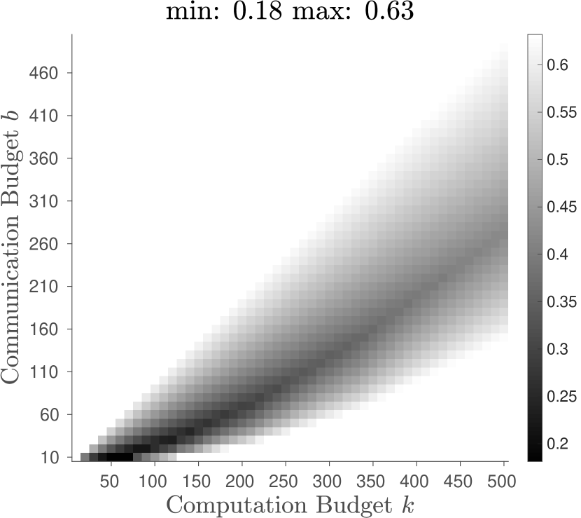
(a) KITTI 00 ($\Delta=41$)

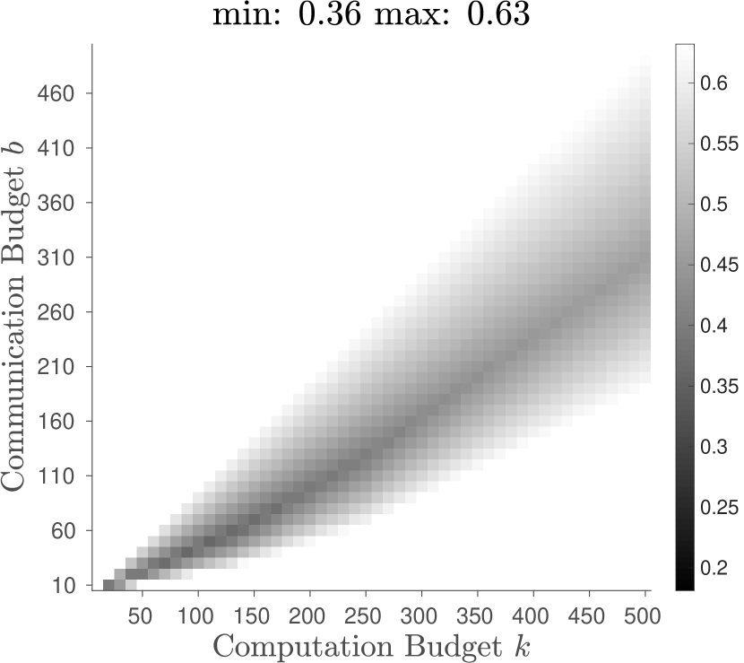
(b) KITTI 00 ($\Delta=5$)

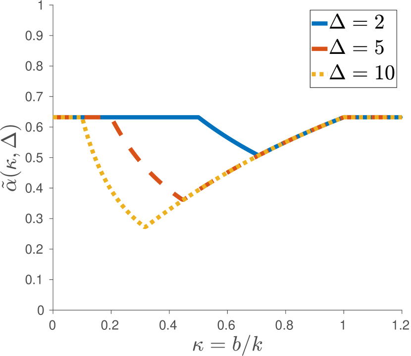
(c) $\tilde{\alpha}(\kappa,\Delta)$

Figure 2: (a) S-Greedy approximation factor in KITTI 00 with $\Delta=41$. The approximation factor in this case varies between $0.18$ and $0.63$. (b) S-Greedy approximation factor in KITTI 00 with the maximum degree capped at $\Delta=5$. The approximation factor varies between $0.36$ and $0.63$. (c) The approximate S-Greedy performance guarantee as a function of $\kappa\triangleq b/k$ with different $\Delta$.

To gain more intuition, let us approximate $\lfloor k/\Delta\rfloor$ in $\alpha(b,k,\Delta)$ with $k/\Delta$. With this simplification, the performance guarantee can be represented as $\tilde{\alpha}(\kappa,\Delta)$, i.e., a function of the budgets ratio $\kappa\triangleq b/k$ and $\Delta$. Figure 2(c) shows $\tilde{\alpha}(\kappa,\Delta)$ as a function of $\kappa$, with different maximum degree $\Delta$ (independent of any specific $\mathcal{G}_{\mathsf{x}}$).

Remark 2

It is worth noting that $\alpha(b,k,\Delta)$ can be bounded from below by a function of $\Delta$, i.e., independent of $b$ and $k$. More precisely, after some algebraic manipulation, it can be shown that $\alpha(b,k,\Delta)\geq 1-\exp(-c(\Delta))$ where $1/(\Delta+1)\leq c(\Delta)\leq 1/\sqrt{\Delta}$. This implies that for a bounded $\Delta\leq\Delta_{\text{max}}$, S-Greedy is a constant-factor approximation algorithm for $\text{P}_{1}$.

5 Experimental Results

Figure 3: Left: KITTI 00; Right: 2D simulation [29]. Each figure shows simulated trajectories of five robots. The KITTI trajectories shown are estimated purely using prior beliefs and odometry measurements (hence the drift). The simulated trajectories shown are the exact ground truth.

(a) KITTI 00

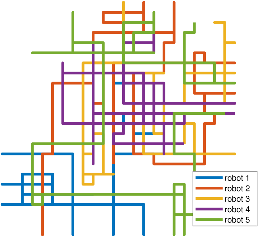
(b) Simulation

We evaluate the proposed algorithms using sequence 00 of the KITTI odometry benchmark [9] and a synthetic Manhattan-like dataset [29]. Each dataset is divided into multiple trajectories to simulate individual robots’ paths (Figure 3). For the KITTI sequence, we project the trajectories to the 2D plane in order to use the tree-connectivity objective [14]. Visual odometry measurements and potential loop closures are obtained from a modified version of ORB-SLAM2 [22]. We estimate the probability of each potential loop closure by normalizing the corresponding DBoW2 score [8]. For any specific environment, better mapping from the similarity score to the corresponding probability can be learned offline. Nonetheless, these estimated probabilities are merely used to encourage the selection of more promising potential matches, and the exact mapping used is orthogonal to the evaluation of the proposed approximation algorithms. For simulation, noisy odometry and loop closures are generated using the 2D simulator of g2o [18]. Each loop closure in the original dataset is considered a potential match with an occurrence probability generated randomly according to the uniform distribution $\mathcal{U}(0,1)$. Then, we decide if each potential match is a “true” loop closure by sampling from a Bernoulli distribution with the corresponding occurrence probability. This process thus provides unbiased estimates of the actual occurrence probabilities.

In our experiments, each visual observation contains about $2000$ keypoints. We ignore the insignificant variation in observation sizes and design all test cases under the TU communication cost regime. Assuming each keypoint (consisting of a descriptor and coordinates) uses $40$ bytes of data, a communication budget of $50$, for example, translates to about $4$MB of data transmission [29].

5.1 Certifying Near-Optimality via Convex Relaxation

Evaluating the proposed algorithms ideally requires access to the optimal value (OPT) of $\text{P}_{1}$. However, computing OPT by brute force is challenging even in relatively small instances. Following [29], we compute an upper bound UPT $\geq$ OPT by solving a natural convex relaxation of $\text{P}_{1}$, and use UPT as a surrogate for OPT. Comparing with UPT provides an a posteriori certificate of near-optimality for solutions returned by the proposed algorithms. Let $\boldsymbol{\pi}\triangleq[\pi_{1},\dots,\pi_{n}]^{\top}$ and $\boldsymbol{\ell}\triangleq[\ell_{1},\dots,\ell_{m}]^{\top}$ be indicator variables corresponding to vertices and edges of $\mathcal{G}_{\mathsf{x}}$, respectively. Let $\mathbf{A}$ be the undirected incidence matrix of $\mathcal{G}_{\mathsf{x}}$. $\text{P}_{1}$ can then be formulated in terms of $\boldsymbol{\pi}$ and $\boldsymbol{\ell}$. For example, for modular objectives (Section 3) under the TU communication model, $\text{P}_{1}$ is equivalent to maximizing $f^{\star}(\boldsymbol{\ell})\triangleq\sum_{e\in\mathcal{E}_{\mathsf{x}}}p(e)\cdot\ell_{e}$ subject to $(\boldsymbol{\pi},\boldsymbol{\ell})\in\mathcal{F}_{\text{int}}$, where $\mathcal{F}_{\text{int}}\triangleq\big{\{}(\boldsymbol{\pi},\boldsymbol{\ell})\in\{0,1\}^{n}\times\{0,1\}^{m}:\mathbf{1}^{\top}\boldsymbol{\pi}\leq b,\mathbf{1}^{\top}\boldsymbol{\ell}\leq k,\mathbf{A}^{\top}\boldsymbol{\pi}\geq\boldsymbol{\ell}\big{\}}$. Relaxing $\mathcal{F}_{\text{int}}$ to $\mathcal{F}\triangleq\big{\{}(\boldsymbol{\pi},\boldsymbol{\ell})\in[0,1]^{n}\times[0,1]^{m}:\mathbf{1}^{\top}\boldsymbol{\pi}\leq b,\mathbf{1}^{\top}\boldsymbol{\ell}\leq k,\mathbf{A}^{\top}\boldsymbol{\pi}\geq\boldsymbol{\ell}\big{\}}$ gives the natural LP relaxation, whose optimal value is an upper bound on OPT. Note that in this special case, we can also compute OPT directly by solving the original ILP (this is not practical for real-world applications). On the other hand, for maximizing the D-criterion and tree-connectivity (Section 4), convex relaxation produces determinant maximization (maxdet) problems [31] subject to affine constraints. In our experiments, all LP and ILP instances are solved using built-in solvers in MATLAB. All maxdet problems are modeled using the YALMIP toolbox [20] and solved using SDPT3 [30] in MATLAB.

5.2 Results with Modular Objectives

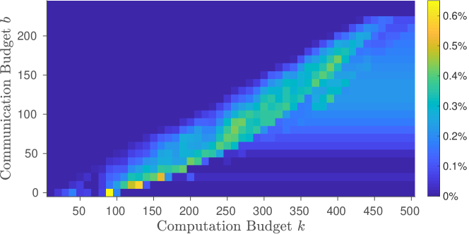
Figure 5: Optimality gap of M-Greedy in KITTI 00 under TU. In this case, the objective is to maximize the expected number of loop closures ([29, Eq. $4$]). For each problem instance specified by a pair of budgets $(b,k)$, we calculate the difference between the achieved value and the optimal value obtained by solving the ILP. Each value is then normalized by the maximum achievable value given infinite budgets and shown in percentage.

For brevity, we refer to the proposed greedy algorithm in Section 3 under TU (see Algorithm 1) as M-Greedy. Figure 5 shows the optimality gap of M-Greedy evaluated on the KITTI 00 dataset. In this case, the objective is to maximize the expected number of true loop closures ([29, Eq. $4$]). Given the exchange graph, we vary the communication budget $b$ and computation budget $k$ to produce different instances of $\text{P}_{1}$. For each instance, we compute the difference between the achieved value and the optimal value obtained by solving the corresponding ILP (Section 5.1). The computed difference is then normalized by the maximum achievable value given infinite budgets and converted into percentage. The result for each instance is shown as an individual cell in Figure 5. In all instances, the optimality gaps are close to zero. In fact, the maximum unnormalized difference across all instances is about $1.35$, i.e., the achieved value and the optimal value only differ by $1.35$ expected loop closures. These results clearly confirm the near-optimal performance of the proposed algorithm. Furthermore, in many instances, M-Greedy finds optimal solutions (shown in dark blue). We note that this result is expected when $b>k$ (top-left region), as in this case $\text{P}_{1}$ reduces to a degenerate instance of the knapsack problem, for which greedy algorithm is known to be optimal.

5.3 Results with Submodular Objectives

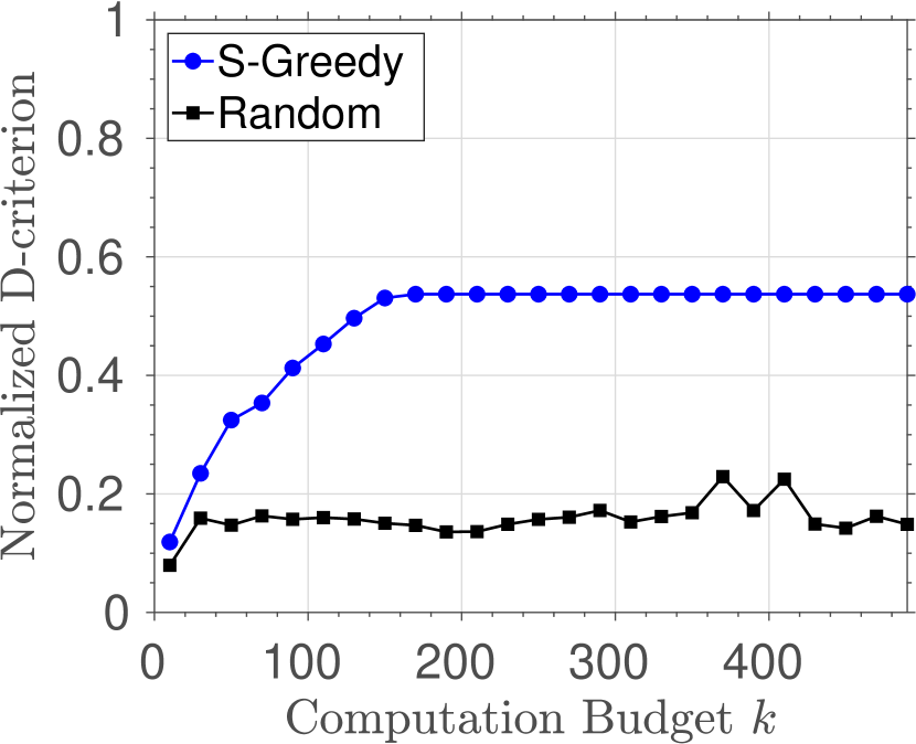
(a) $b=20$

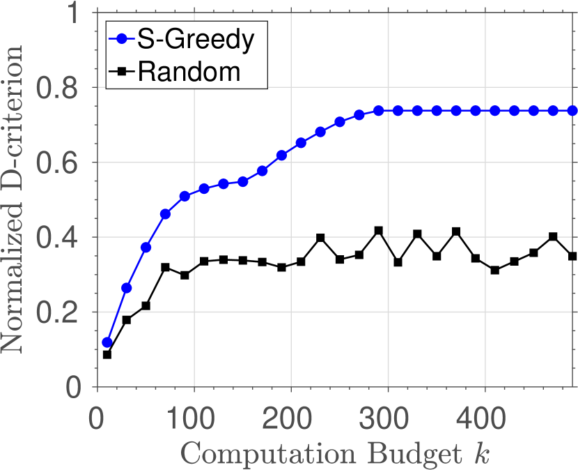
(b) $b=70$

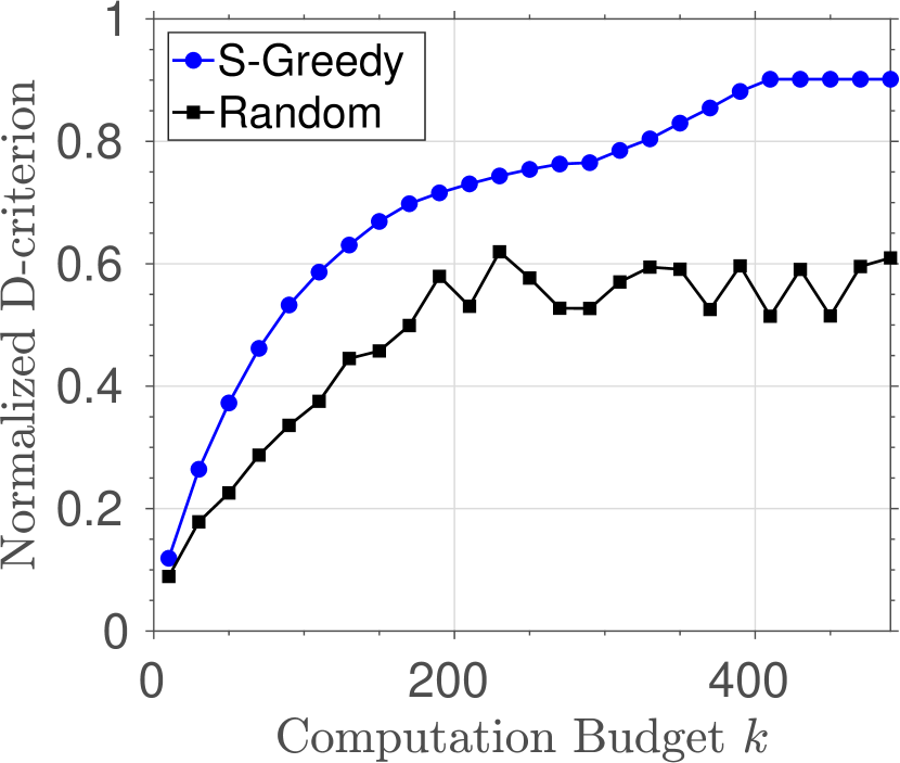
(c) $b=150$

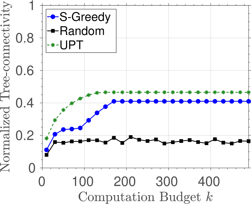
(d) $b=20$

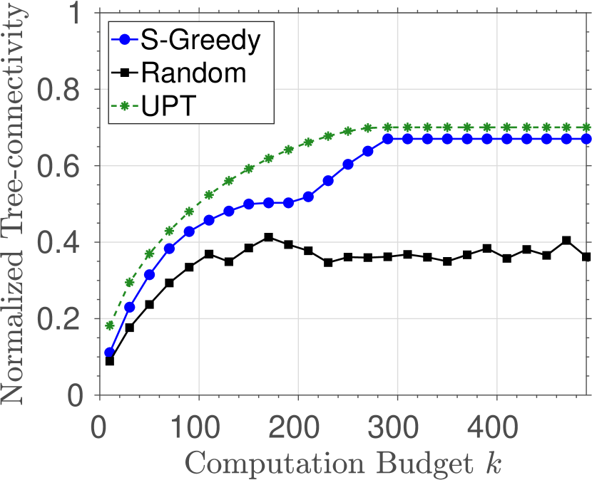
(e) $b=70$

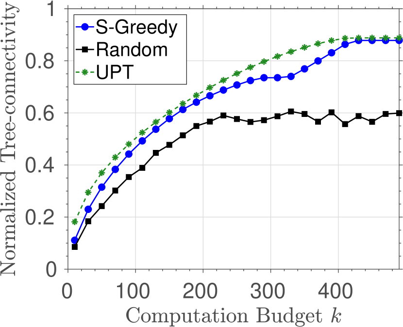
(f) $b=150$

Figure 6: Performance of Submodular-Greedy in KITTI 00 under TU, with the D-criterion objective in (a)-(c) and tree-connectivity objective in (d)-(f). Each figure shows one scenario with a fixed communication budget $b$ and varying computation budget $k$. The proposed algorithm is compared against a random baseline. With the tree-connectivity objective, we also show the upper bound (UPT) computed using convex relaxation. All values are normalized by the maximum achievable value given infinite budgets.

Figure 6 shows performance of S-Greedy in KITTI 00 under the TU regime. Figures 6(a)-6(c) use the D-criterion objective [29, Eq. $2$], and 6(d)-6(f) use the tree-connectivity objective [29, Eq. $3$]. Each figure corresponds to one scenario with a fixed communication budget $b$ and varying computation budget $k$. We compare the proposed algorithm with a baseline that randomly selects $b$ vertices, and then selects $k$ edges at random from the set of edges incident to the selected vertices. When using the tree-connectivity objective, we also plot the upper bound (UPT) computed using convex relaxation (Section 5.1). All values shown are normalized by the maximum achievable value given infinite budgets. In all instances, S-Greedy clearly outperforms the random baseline. Moreover, in 6(d)-6(f), the achieved objective values are close to UPT. In particular, using the fact that UPT $\geq$ OPT, we compute a lower bound on the empirical approximation ratio in 6(d)-6(f), which varies between $0.58$ and $0.99$. This confirms the near-optimality of the approximate solutions found by S-Greedy. The inflection point of each S-Greedy curve in Figure 6(a)-6(f) corresponds to the point where the algorithm switches from greedily selecting edges (E-Greedy) to greedily selecting vertices (V-Greedy). Note that in all scenarios, the achieved value of S-Greedy eventually saturates. This is because as $k$ increases, S-Greedy eventually spends the entire communication budget and halts. In these cases, since we already select the maximum number (i.e., $b$) of vertices, the algorithm achieves a constant approximation factor of $1-1/e$ (see Lemma 4 in Appendix H). Due to space limitation, additional results on the simulated datasets and results comparing M-Greedy with S-Greedy in the case of modular objectives are reported in Appendix I.

6 Conclusion

Inter-robot loop closure detection is a critical component for many multirobot applications, including those that require collaborative localization and mapping. The resource-intensive nature of this process, together with the limited nature of mission-critical resources available on-board necessitate intelligent utilization of available/allocated resources. This paper studied distributed inter-robot loop closure detection under computation and communication budgets. More specifically, we sought to maximize monotone submodular performance metrics by selecting a subset of potential inter-robot loop closures that is feasible with respect to both computation and communication budgets. This problem generalizes previously studied NP-hard problems that assume either unbounded computation or communication.

In particular, for monotone modular objectives (e.g., expected number of true loop closures) we presented a family of greedy algorithms with constant-factor approximation ratios under multiple communication cost regimes. This was made possible through establishing an approximation-factor preserving reduction to well-studied instances of monotone submodular maximization problems under cardinality, knapsack, and partition matroid constraints. More generally, for any monotone submodular objective, we presented an approximation algorithm that exploits the complementary nature of greedily selecting potential loop closures for verification and greedily broadcasting observations, in order to establish a performance guarantee. The performance guarantee in this more general case depends on resource budgets and the extent of perceptual ambiguity.

It remains an open problem whether constant-factor approximation for any monotone submodular objective is possible. We plan to study this open problem as part of our future work. Additionally, although the burden of verifying potential loop closures is distributed among the robots, our current framework still relies on a centralized scheme for evaluating the performance metric and running the approximation algorithms presented for $\text{P}_{1}$. In the future, we aim to eliminate such reliance on centralized computation.

Acknowledgments

This work was supported in part by the NASA Convergent Aeronautics Solutions project Design Environment for Novel Vertical Lift Vehicles (DELIVER), by ONR under BRC award N000141712072, and by ARL DCIST under Cooperative Agreement Number W911NF-17-2-0181.

Appendix G Algorithms

Algorithm 1 Modular-Greedy (TU)

1:

2:- Exchange graph $\mathcal{G}_{\mathsf{x}}=(\mathcal{V}_{\mathsf{x}},\mathcal{E}_{\mathsf{x}})$

3:- Communication budget $b$ and computation budget $k$

4:- Modular $f:2^{\mathcal{E}_{\mathsf{x}}}\to\mathbb{R}_{\geq 0}$ and $g$ as defined in Section 3

5:

6:- A budget-feasible pair $\mathcal{V}_{\text{grd}}\subseteq\mathcal{V}_{\mathsf{x}},\mathcal{E}_{\text{grd}}\subseteq\mathcal{E}_{\mathsf{x}}$.

7:$\mathcal{V}_{\text{grd}}\leftarrow\varnothing$

8:for $i=1:b$ do $\triangleright$ greedy loop

9:     $v^{\star}\leftarrow\operatorname*{arg\,max}_{v\in\mathcal{V}_{\mathsf{x}}\setminus\mathcal{V}_{\text{grd}}}g(\mathcal{V}_{\text{grd}}\cup\{v\})$

10:     $\mathcal{V}_{\text{grd}}\leftarrow\mathcal{V}_{\text{grd}}\cup\{v^{\star}\}$

11:end for

12:$\mathcal{E}_{\text{grd}}\leftarrow\mathsf{edges}(\mathcal{V}_{\text{grd}})$

13:return $\mathcal{V}_{\text{grd}},\mathcal{E}_{\text{grd}}$

Algorithm 2 Edge-Greedy (TU)

1:

2:- Exchange graph $\mathcal{G}_{\mathsf{x}}=(\mathcal{V}_{\mathsf{x}},\mathcal{E}_{\mathsf{x}})$

3:- Communication budget $b$ and computation budget $k$

4:- $f:2^{\mathcal{E}_{\mathsf{x}}}\to\mathbb{R}_{\geq 0}$

5:

6:- A budget-feasible pair $\mathcal{V}_{\text{grd}}\subseteq\mathcal{V}_{\mathsf{x}},\mathcal{E}_{\text{grd}}\subseteq\mathcal{E}_{\mathsf{x}}$.

7:$\mathcal{E}_{\text{grd}}\leftarrow\varnothing$

8:for $i=1:\min(b,k)$ do $\triangleright$ greedy loop

9:     $e^{\star}\leftarrow\operatorname*{arg\,max}_{e\in\mathcal{E}_{\mathsf{x}}\setminus\mathcal{E}_{\text{grd}}}f(\mathcal{E}_{\text{grd}}\cup\{e\})$

10:     $\mathcal{E}_{\text{grd}}\leftarrow\mathcal{E}_{\text{grd}}\cup\{e^{\star}\}$

11:end for

12:$\mathcal{V}_{\text{grd}}\leftarrow\textsc{\small VertexCover}(\mathcal{E}_{\text{grd}})$ $\triangleright$ any vertex cover of $\mathcal{E}_{\text{grd}}$

13:if $k>b$ then $\triangleright$ local optimization

14:     $\mathcal{E}_{\text{free}}\leftarrow\mathsf{edges}(\mathcal{V}_{\text{grd}})\setminus\mathcal{E}_{\text{grd}}$ $\triangleright$ identify comm-free edges

15:     for $i=1:\min(|\mathcal{E}_{\text{free}}|,k-b)$ do

16:         $e^{\star}\leftarrow\operatorname*{arg\,max}_{e\in\mathcal{E}_{\text{free}}\setminus\mathcal{E}_{\text{grd}}}f(\mathcal{E}_{\text{grd}}\cup\{e\})$

17:         $\mathcal{E}_{\text{grd}}\leftarrow\mathcal{E}_{\text{grd}}\cup\{e^{\star}\}$

18:     end for

19:end if

20:return $\mathcal{V}_{\text{grd}},\mathcal{E}_{\text{grd}}$

Algorithm 3 Vertex-Greedy (TU)

1:

2:- Exchange graph $\mathcal{G}_{\mathsf{x}}=(\mathcal{V}_{\mathsf{x}},\mathcal{E}_{\mathsf{x}})$

3:- Communication budget $b$ and computation budget $k$

4:- $f:2^{\mathcal{E}_{\mathsf{x}}}\to\mathbb{R}_{\geq 0}$ and $g:\mathcal{V}\mapsto f\big{(}\mathsf{edges}(\mathcal{V})\big{)}$

5:

6:- A budget-feasible pair $\mathcal{V}_{\text{grd}}\subseteq\mathcal{V}_{\mathsf{x}},\mathcal{E}_{\text{grd}}\subseteq\mathcal{E}_{\mathsf{x}}$.

7:$\mathcal{V}_{\text{grd}}\leftarrow\varnothing$

8:while True do $\triangleright$ greedy loop

9:     $v^{\star}\leftarrow\operatorname*{arg\,max}_{v\in\mathcal{V}_{\mathsf{x}}\setminus\mathcal{V}_{\text{grd}}}g(\mathcal{V}_{\text{grd}}\cup\{v\})$ $\triangleright$ find next best vertex

10:     if $|\mathcal{V}_{\text{grd}}\cup\{v^{\star}\}|>b$ or $|\mathsf{edges}(\mathcal{V}_{\text{grd}}\cup\{v^{\star}\})|>k$  then

11:         break $\triangleright$ stop if violating budget

12:     end if

13:     $\mathcal{V}_{\text{grd}}\leftarrow\mathcal{V}_{\text{grd}}\cup\{v^{\star}\}$

14:end while

15:$\mathcal{E}_{\text{grd}}\leftarrow\mathsf{edges}(\mathcal{V}_{\text{grd}})$

16:return $\mathcal{V}_{\text{grd}},\mathcal{E}_{\text{grd}}$

Appendix H Proofs

Proof (Theorem 3.1)

For convenience, we present the proof after modifying the definition of $g$ according to

$$g(\mathcal{V})=\underset{\mathcal{E}\subseteq\mathsf{edges}(\mathcal{V})\cup\mathcal{N}}{\max}\hskip 2.84544pt\sum_{e\in\mathcal{E}}p(e)\quad\text{s.t.}\quad|\mathcal{E}|=k$$ (1)

where now $\mathcal{N}$ is a set of $k$ null items with $p(e)=0$ for all $e\in\mathcal{N}$. It is easy to see this modification does not change the function $g$.

• Normalized: $g(\varnothing)=0$ by definition.

• Monotone: for any $\mathcal{S}\subseteq\mathcal{Q}\subseteq\mathcal{V}_{\mathsf{x}}$, $\mathsf{edges}(\mathcal{S})\subseteq\mathsf{edges}(\mathcal{Q})$ and thus $g(\mathcal{S})\leq g(\mathcal{Q})$.

• Submodular: we need to show that for any $\mathcal{S}\subseteq\mathcal{Q}\subseteq\mathcal{V}_{\mathsf{x}}$ and all $v\in\mathcal{V}_{\mathsf{x}}/\mathcal{Q}$:

  $$g(\mathcal{S}\cup\{v\})-g(\mathcal{S})\geq g(\mathcal{Q}\cup\{v\})-g(\mathcal{Q})$$ (2)

  If $g(\mathcal{Q}\cup\{v\})=g(\mathcal{Q})$, (2) follows from the monotonicity of $g$. We thus focus on cases where $g(\mathcal{Q}\cup\{v\})>g(\mathcal{Q})$. Recall that for any $\mathcal{V}\subseteq\mathcal{V}_{\mathsf{x}}$, $g(\mathcal{V})$ is the sum of top $k$ edge probabilities in $\mathsf{edges}(\mathcal{V})\cup\mathcal{N}$. Let $\mathsf{edges}(\mathcal{V};k)$ represent such a set. We have,

  $$g(\mathcal{Q}\cup\{v\})-g(\mathcal{Q}) =\sum_{e\in\mathcal{E}_{\boxplus}}p(e)-\sum_{e\in\mathcal{E}_{\boxminus}}p(e)$$ (3)

  where $\mathcal{E}_{\boxplus}\triangleq\mathsf{edges}(\mathcal{Q}\cup\{v\};k)\setminus\mathsf{edges}(\mathcal{Q};k)$ and $\mathcal{E}_{\boxminus}\triangleq\mathsf{edges}(\mathcal{Q};k)\setminus\mathsf{edges}(\mathcal{Q}\cup\{v\};k)$. We know that $|\mathcal{E}_{\boxplus}|=|\mathcal{E}_{\boxminus}|$ since $|\mathsf{edges}(\mathcal{Q}\cup\{v\};k)|=|\mathsf{edges}(\mathcal{Q};k)|=k$. Now we claim that,

  $$g(\mathcal{S}\cup\{v\})\geq g(\mathcal{S})+\sum_{e\in\mathcal{E}_{\boxplus}}p(e)-\sum_{e\in\mathcal{E}_{\boxminus}^{\ast}}p(e)$$ (4)

  in which $\mathcal{E}_{\boxminus}^{\ast}$ is the set of $|\mathcal{E}_{\boxplus}|$ edges in $\mathsf{edges}(\mathcal{S};k)$ with lowest probabilities. To see this, note that $\mathsf{edges}(\mathcal{S};k)\cup\mathcal{E}_{\boxplus}\setminus\mathcal{E}^{\ast}_{\boxminus}$ is a $k$-subset of $\mathsf{edges}(\mathcal{S}\cup\{v\})\cup\mathcal{N}$. Therefore,

  $$g(\mathcal{S}\cup\{v\}) \triangleq\underset{\mathcal{E}\subseteq\mathsf{edges}(\mathcal{V})\cup\mathcal{N}}{\max}\hskip 2.84544pt\sum_{e\in\mathcal{E}}p(e)\quad\text{s.t.}\quad|\mathcal{E}|=k$$ (5)

  $$\geq\sum_{e\in\mathsf{edges}(\mathcal{S};k)\cup\mathcal{E}_{\boxplus}\setminus\mathcal{E}^{\ast}_{\boxminus}}p(e)$$ (6)

  $$=g(\mathcal{S})+\sum_{e\in\mathcal{E}_{\boxplus}}p(e)-\sum_{e\in\mathcal{E}_{\boxminus}^{\ast}}p(e)$$ (7)

  Now let us sort edges according to their probabilities in $\mathsf{edges}(\mathcal{S};k)$ and in $\mathsf{edges}(\mathcal{Q};k)$. Since $\mathcal{S}\subseteq\mathcal{Q}$ and, consequently, $\mathsf{edges}(\mathcal{S})\subseteq\mathsf{edges}(\mathcal{Q})$, the probability of the $i$th most-probable edge in $\mathsf{edges}(\mathcal{Q};k)$ is at least that of the $i$th most-probable edge in $\mathsf{edges}(\mathcal{S};k)$. This shows that $\sum_{e\in\mathcal{E}_{\boxminus}}p(e)\geq\sum_{e\in\mathcal{E}_{\boxminus}^{\ast}}p(e)$, which together with (3) and (4) conclude the proof.

Lemma 1

For any $\mathcal{V}\subseteq\mathcal{V}_{\mathsf{x}}$ that is $\text{P}_{2}$-feasible, define

$$\mathsf{edges}(\mathcal{V};k)\in\underset{\mathcal{E}\subseteq\mathsf{edges}(\mathcal{V})}{\operatorname*{arg\,max}}f(\mathcal{E})\text{ s.t. }|\mathcal{E}|\leq k.$$ (8)

Then, $\mathsf{edges}(\mathcal{V};k)$ is $\text{P}_{1}$-feasible.

Proof (Lemma 8)

By construction, $|\mathsf{edges}(\mathcal{V};k)|\leq k$. Also, there exists a cover of $\mathsf{edges}(\mathcal{V};k)$ (namely, $\mathcal{V}$) that satisfies CB. This concludes the proof.

Lemma 2

Let OPT₁ and OPT₂ denote the optimal values of $\text{P}_{1}$ and $\text{P}_{2}$, respectively. Then $\text{\text{OPT}${}_{1}$}=\text{\text{OPT}${}_{2}$}$.

Proof (Lemma 2)

We prove $\text{\text{OPT}${}_{1}$}\geq\text{\text{OPT}${}_{2}$}$ and $\text{\text{OPT}${}_{2}$}\geq\text{\text{OPT}${}_{1}$}$.

• $\text{\text{OPT}${}_{1}$}\geq\text{\text{OPT}${}_{2}$}$: Suppose $\mathcal{V}^{\star}$ is an optimal solution to $\text{P}_{2}$. Let $\mathcal{E}^{\star}\triangleq\mathsf{edges}(\mathcal{V}^{\star};k)$. By Lemma 8, $\mathcal{E}^{\star}$ is $\text{P}_{1}$-feasible. In addition, $f(\mathcal{E}^{\star})=\text{\text{OPT}${}_{2}$}$ by the definition of $g$. Therefore, $\text{\text{OPT}${}_{1}$}\geq f(\mathcal{E}^{\star})=\text{\text{OPT}${}_{2}$}$.

• $\text{\text{OPT}${}_{2}$}\geq\text{\text{OPT}${}_{1}$}$: Suppose $\mathcal{E}^{\star}$ is an optimal solution to $\text{P}_{1}$. Then there exists $\mathcal{V}^{\star}\in\mathsf{cover}(\mathcal{E}^{\star})$ that satisfies CB. Thus $\mathcal{V}^{\star}$ is $\text{P}_{2}$-feasible. Also, $g(\mathcal{V}^{\star})\geq\text{\text{OPT}${}_{1}$}$ by the definition of $g$. Therefore, $\text{\text{OPT}${}_{2}$}\geq g(\mathcal{V}^{\star})\geq\text{\text{OPT}${}_{1}$}$.

Proof (Theorem 3.2)

Let $\tilde{\mathcal{E}}$ be the edge set returned by the procedure. By Lemma 8, $\tilde{\mathcal{E}}$ is $\text{P}_{1}$-feasible. Now,

$$f(\tilde{\mathcal{E}}) =g(\mathcal{V}) g$$ (def. of ) (9)

$$\geq\alpha\cdot\text{\text{OPT}${}_{2}$}$$ (assumption on ALG) (10)

$$=\alpha\cdot\text{\text{OPT}${}_{1}$}.$$ (Lemma 2) (11)

Lemma 3

Edge-Greedy (Algorithm 2) is an $\alpha_{e}(b,k)$-approximation algorithm for $\text{P}_{1}$ under TU, where

$$\alpha_{e}(b,k)\triangleq 1-\exp\big{(}-\min\,\{1,b/k\}\big{)}.$$ (12)

Proof (Lemma 3)

We first show that Algorithm 2 returns a feasible solution to $\text{P}_{1}$. The algorithm proceeds in two phases. In phase I (line 8-12), we greedily select $\min(b,k)$ edges. This clearly satisfies the computation budget $k$. Then, we find an arbitrary vertex cover of the selected edges (line 12), e.g., by selecting one of the two vertices for each edge. For the rest of the algorithm, we fix this vertex cover as the subset of vertices we return. Note that in the worst case, the selected edges will be disjoint. Consequently, the size of the vertex cover is at most $\min(b,k)$, satisfying the communication budget $b$. Thus, by the end of phase I, the constructed solution is $\text{P}_{1}$-feasible.

Phase II (line 13-19) improves the current solution while ensuring feasibility. Given the selected vertices, we identify the set of unselected edges that are “communication-free”, i.e., no extra communication cost will be incurred if we select any of these edges. In other words, an edge is “communication-free” if it is already covered by the current vertex cover. In Phase II, the algorithm simply adds “communication-free” edges greedily, until there is no computation budget left. The final solution thus remains $\text{P}_{1}$-feasible.

Next, we prove the performance guarantee presented in the lemma. To do so, we only need to look at the solution after Phase I. Let OPT₁ denote the optimal value of $\text{P}_{1}$. Consider the relaxed version of $\text{P}_{1}$ where we remove the communication budget,

$$\underset{\mathcal{E}\subseteq\mathcal{E}_{\mathsf{x}}}{\text{maximize }}f(\mathcal{E})\text{ s.t. }|\mathcal{E}|\leq k.$$ (13)

Let OPT_e denote the optimal value of the relaxed problem. Clearly, OPT_e $\geq\text{\text{OPT}${}_{1}$}$. Let $\mathcal{E}_{\text{grd}}$ be the set of selected edges after Phase I. By construction, $|\mathcal{E}_{\text{grd}}|\geq\min(b,k)$. Thus,

$$f(\mathcal{E}_{\text{grd}}) \geq\Big{(}1-\exp\big{(}-\min\{b,k\}/k\big{)}\Big{)}\cdot\text{\text{OPT}${}_{e}$} 1.5$$ ([16, Theorem ]) (14)

$$=\alpha_{e}(b,k)\cdot\text{\text{OPT}${}_{e}$} \alpha_{e}$$ (def. of ) (15)

$$\geq\alpha_{e}(b,k)\cdot\text{\text{OPT}${}_{1}$}. {}_{e}\geq\text{\text{OPT}${}_{1}$}$$ (OPT) (16)

Finally, note that because of Phase II, $\min(b,k)$ is only a lower bound on the number of edges selected by E-Greedy.

Lemma 4

Let $\Delta$ be the maximum vertex degree in $\mathcal{G}_{\mathsf{x}}$. Vertex-Greedy (Algorithm 3) is an $\alpha_{v}(b,k,\Delta)$-approximation algorithm for $\text{P}_{1}$ under TU, where

$$\alpha_{v}(b,k,\Delta) \triangleq 1-\exp\big{(}-\min\,\{1,\lfloor k/\Delta\rfloor/b\}\big{)}.$$ (17)

Proof (Lemma 4)

As shown in Algorithm 3, we terminate the greedy loop if the next selected vertex violates either one of the budgets (line 11). Thus, the returned solution is guaranteed to be $\text{P}_{1}$-feasible. Note that the number of vertices we select is at least $\min(b,\lfloor k/\Delta\rfloor)$. This is because whenever we select less than this number of vertices, there is guaranteed to be enough computation and communication budgets to select the next vertex and include all its incident edges.

Next, we prove the performance guarantee presented in the lemma. Let OPT₁ denote the optimal value of $\text{P}_{1}$. Consider the relaxed version of $\text{P}_{1}$ under TU where we remove the computation budget,

$$\underset{\mathcal{E}\subseteq\mathcal{E}_{\mathsf{x}}}{\text{maximize }}f(\mathcal{E})\text{ s.t. }\exists\,\mathcal{V}\in\mathsf{cover}(\mathcal{E})\text{ s.t. }|\mathcal{V}|\leq b.$$ (18)

By [29, Theorem $2$], there is an approximation-preserving reduction from the above problem to the following problem,

$$\underset{\mathcal{V}\subseteq\mathcal{V}_{\mathsf{x}}}{\text{maximize }}h(\mathcal{V})\text{ s.t. }|\mathcal{V}|\leq b.$$ (19)

where $h:2^{\mathcal{V}_{\mathsf{x}}}\to\mathbb{R}_{\geq 0}:\mathcal{V}\mapsto f(\mathsf{edges}(\mathcal{V}))$. Let OPT_v and OPT${}^{\prime}_{v}$ denote the optimal values of (18) and (19), respectively. By [29, Lemma $1.2$], OPT_v $=$ OPT${}^{\prime}_{v}$. Clearly, OPT_v $\geq\text{\text{OPT}${}_{1}$}$. Let $\mathcal{E}_{\text{grd}},\mathcal{V}_{\text{grd}}$ be the edges and vertices selected by Vertex-Greedy. By construction, $|\mathcal{V}_{\text{grd}}|\geq\min(b,\lfloor k/\Delta\rfloor)$. Thus,

$$f(\mathcal{E}_{\text{grd}}) =h(\mathcal{V}_{\text{grd}}) h$$ (def. of ) (20)

$$\geq\Big{(}1-\exp\big{(}-\frac{\min\{b,\lfloor k/\Delta\rfloor\}}{b}\big{)}\Big{)}\cdot\text{\text{OPT}${}^{\prime}_{v}$} 1.5$$ ([16, Theorem ]) (21)

$$=\alpha_{v}(b,k,\Delta)\cdot\text{\text{OPT}${}^{\prime}_{v}$} \alpha_{v}$$ (def. of ) (22)

$$=\alpha_{v}(b,k,\Delta)\cdot\text{\text{OPT}${}_{v}$} 1.2$$ ([29, Lemma ]) (23)

$$\geq\alpha_{v}(b,k,\Delta)\cdot\text{\text{OPT}${}_{1}$}. {}_{v}\geq\text{\text{OPT}${}_{1}$}$$ (OPT) (24)

As mentioned above, $\min(b,\lfloor k/\Delta\rfloor)$ is only a lower bound on the number of vertices selected by V-Greedy.

Proof (Theorem 4.1)

By Lemma 3 and Lemma 4,

$$\alpha(b,k,\Delta) =\max\,\{\alpha_{e}(b,k),\alpha_{v}(b,k,\Delta)\}$$ (25)

$$=1-\exp\big{(}-\min\big{\{}1,\max\,(b/k,\lfloor k/\Delta\rfloor/b)\big{\}}\big{)}$$ (26)

$$=1-\exp\big{(}-\min\{1,\gamma\}\big{)}.$$ (27)

Appendix I Additional Results

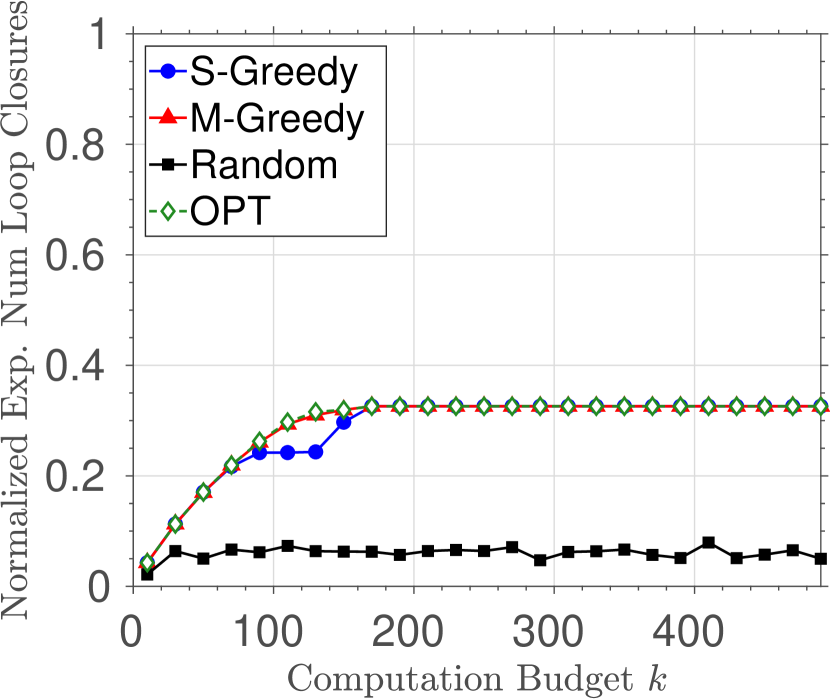
(a) $b=20$

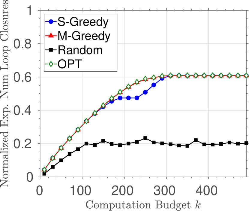
(b) $b=70$

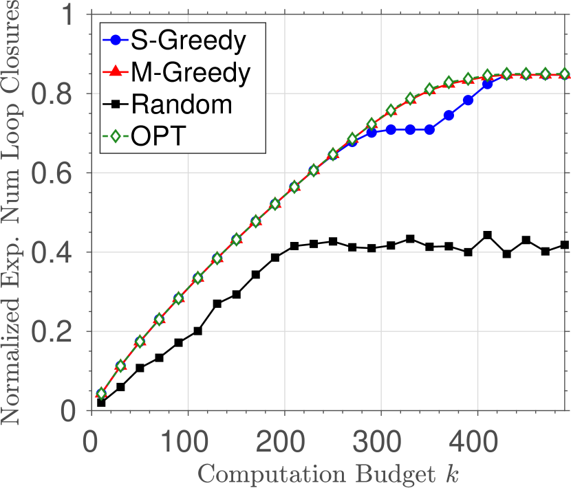
(c) $b=150$

Figure 7: Comparison of M-Greedy and S-Greedy when maximizing the expected number of true loop closures in KITTI 00. Each subplot shows one scenario with a fixed communication budget $b$ and varying computation budget $k$. For completeness we also include the random baseline and the optimal values (OPT) computed by solving the corresponding ILP.

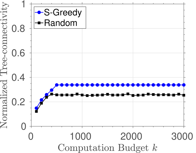
(a) $b=50$

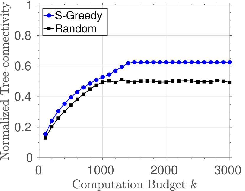
(b) $b=150$

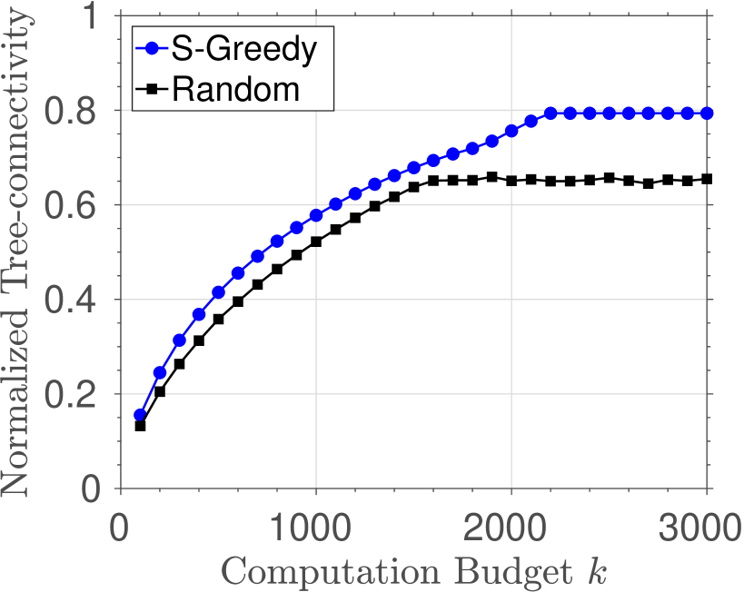
(c) $b=250$

Figure 8: Performance of Submodular-Greedy in simulation under the TU regime, with the tree-connectivity objective. Each subplot shows one scenario with a fixed communication budget $b$ and varying computation budget $k$. The proposed algorithm is compared against a random baseline. In this case, we do not compute the upper bound (UPT) using convex relaxation as it is too time-consuming.

References

- Calinescu et al. [2011] G. Calinescu, C. Chekuri, M. Pál, and J. Vondrák. Maximizing a monotone submodular function subject to a matroid constraint. SIAM Journal on Computing, 40(6):1740–1766, 2011. doi: 10.1137/080733991.
- Carlone and Karaman [2017] Luca Carlone and Sertac Karaman. Attention and anticipation in fast visual-inertial navigation. In Robotics and Automation (ICRA), 2017 IEEE International Conference on, pages 3886–3893. IEEE, 2017.
- Choudhary et al. [2017] Siddharth Choudhary, Luca Carlone, Carlos Nieto, John Rogers, Henrik I Christensen, and Frank Dellaert. Distributed mapping with privacy and communication constraints: Lightweight algorithms and object-based models. The International Journal of Robotics Research, 36(12):1286–1311, 2017. doi: 10.1177/0278364917732640.
- Cieslewski and Scaramuzza [2017] Titus Cieslewski and Davide Scaramuzza. Efficient decentralized visual place recognition using a distributed inverted index. IEEE Robotics and Automation Letters, 2(2):640–647, 2017.
- Cieslewski et al. [2017] Titus Cieslewski, Siddharth Choudhary, and Davide Scaramuzza. Data-efficient decentralized visual SLAM. CoRR, abs/1710.05772, 2017.
- [6] Andrew J Davison. Active search for real-time vision. In Computer Vision, 2005. ICCV 2005. Tenth IEEE International Conference on, volume 1, pages 66–73.
- Fisher et al. [1978] Marshall L Fisher, George L Nemhauser, and Laurence A Wolsey. An analysis of approximations for maximizing submodular set functions—ii. In Polyhedral combinatorics, pages 73–87. Springer, 1978.
- Gálvez-López and Tardós [2012] Dorian Gálvez-López and J. D. Tardós. Bags of binary words for fast place recognition in image sequences. IEEE Transactions on Robotics, 28(5):1188–1197, October 2012. ISSN 1552-3098. doi: 10.1109/TRO.2012.2197158.
- Geiger et al. [2012] Andreas Geiger, Philip Lenz, and Raquel Urtasun. Are we ready for autonomous driving? the kitti vision benchmark suite. In Conference on Computer Vision and Pattern Recognition (CVPR), 2012.
- Giamou et al. [2018] Matthew Giamou, Kasra Khosoussi, and Jonathan P How. Talk resource-efficiently to me: Optimal communication planning for distributed loop closure detection. In IEEE International Conference on Robotics and Automation (ICRA), 2018.
- Heinly et al. [2015] Jared Heinly, Johannes Lutz Schönberger, Enrique Dunn, and Jan-Michael Frahm. Reconstructing the World* in Six Days *(As Captured by the Yahoo 100 Million Image Dataset). In Computer Vision and Pattern Recognition (CVPR), 2015.
- Ila et al. [2010] Viorela Ila, Josep M Porta, and Juan Andrade-Cetto. Information-based compact pose SLAM. Robotics, IEEE Transactions on, 26(1):78–93, 2010.
- Joshi and Boyd [2009] Siddharth Joshi and Stephen Boyd. Sensor selection via convex optimization. Signal Processing, IEEE Transactions on, 57(2):451–462, 2009.
- Khosoussi et al. [2016] Kasra Khosoussi, Gaurav S. Sukhatme, Shoudong Huang, and Gamini Dissanayake. Designing sparse reliable pose-graph SLAM: A graph-theoretic approach. International Workshop on the Algorithmic Foundations of Robotics, 2016.
- Khosoussi et al. [2019] Kasra Khosoussi, Matthew Giamou, Gaurav S Sukhatme, Shoudong Huang, Gamini Dissanayake, and Jonathan P How. Reliable graphs for SLAM. International Journal of Robotics Research, 2019. To appear.
- Krause and Golovin [2014] Andreas Krause and Daniel Golovin. Submodular function maximization. In Lucas Bordeaux, Youssef Hamadi, and Pushmeet Kohli, editors, Tractability: Practical Approaches to Hard Problems, pages 71–104. Cambridge University Press, 2014. ISBN 9781139177801.
- Kulik et al. [2009] Ariel Kulik, Hadas Shachnai, and Tami Tamir. Maximizing submodular set functions subject to multiple linear constraints. In Proceedings of the Twentieth Annual ACM-SIAM Symposium on Discrete Algorithms, SODA ’09, pages 545–554, Philadelphia, PA, USA, 2009. Society for Industrial and Applied Mathematics.
- Kümmerle et al. [2011] Rainer Kümmerle, Giorgio Grisetti, Hauke Strasdat, Kurt Konolige, and Wolfram Burgard. g 2 o: A general framework for graph optimization. In Robotics and Automation (ICRA), 2011 IEEE International Conference on, pages 3607–3613. IEEE, 2011.
- Leskovec et al. [2007] Jure Leskovec, Andreas Krause, Carlos Guestrin, Christos Faloutsos, Jeanne VanBriesen, and Natalie Glance. Cost-effective outbreak detection in networks. In Proceedings of the 13th ACM SIGKDD international conference on Knowledge discovery and data mining, pages 420–429. ACM, 2007.
- Löfberg [2004] J. Löfberg. Yalmip : A toolbox for modeling and optimization in matlab. In In Proceedings of the CACSD Conference, Taipei, Taiwan, 2004.
- Minoux [1978] Michel Minoux. Accelerated greedy algorithms for maximizing submodular set functions. In Optimization techniques, pages 234–243. Springer, 1978.
- Mur-Artal and Tardós [2017] Raúl Mur-Artal and Juan D. Tardós. ORB-SLAM2: an open-source SLAM system for monocular, stereo and RGB-D cameras. IEEE Transactions on Robotics, 33(5):1255–1262, 2017. doi: 10.1109/TRO.2017.2705103.
- Nemhauser et al. [1978] George L Nemhauser, Laurence A Wolsey, and Marshall L Fisher. An analysis of approximations for maximizing submodular set functions—i. Mathematical Programming, 14(1):265–294, 1978.
- Paull et al. [2016] Liam Paull, Guoquan Huang, and John J Leonard. A unified resource-constrained framework for graph SLAM. In Robotics and Automation (ICRA), 2016 IEEE International Conference on, pages 1346–1353. IEEE, 2016.
- Pukelsheim [1993] Friedrich Pukelsheim. Optimal design of experiments, volume 50. SIAM, 1993.
- Raguram et al. [2012] Rahul Raguram, Joseph Tighe, and Jan Michael Frahm. Improved geometric verification for large scale landmark image collections. In BMVC 2012 - Electronic Proceedings of the British Machine Vision Conference 2012. British Machine Vision Association, BMVA, 2012. doi: 10.5244/C.26.77.
- Shamaiah et al. [2010] Manohar Shamaiah, Siddhartha Banerjee, and Haris Vikalo. Greedy sensor selection: Leveraging submodularity. In 49th IEEE Conference on Decision and Control (CDC), pages 2572–2577. IEEE, 2010.
- Sviridenko [2004] Maxim Sviridenko. A note on maximizing a submodular set function subject to a knapsack constraint. Operations Research Letters, 32(1):41–43, 2004.
- Tian et al. [2018] Yulun Tian, Kasra Khosoussi, Matthew Giamou, Jonathan P How, and Jonathan Kelly. Near-optimal budgeted data exchange for distributed loop closure detection. In Proceedings of Robotics: Science and Systems, Pittsburgh, USA, June 2018.
- Toh et al. [1999] K. C. Toh, M.J. Todd, and R. H. Tütüncü. SDPT3 – a matlab software package for semidefinite programming. Optimization Methods and Software, 11:545–581, 1999.
- Vandenberghe et al. [1998] Lieven Vandenberghe, Stephen Boyd, and Shao-Po Wu. Determinant maximization with linear matrix inequality constraints. SIAM journal on matrix analysis and applications, 19(2):499–533, 1998.