Optomechanical Gigahertz Oscillator made of a Two Photon Absorption free piezoelectric III/V semiconductor

Abstract

Oscillators in the GHz frequency range are key building blocks for telecommunication and positioning applications. Operating directly in the GHz while keeping high frequency stability and compactness, is still an up-to-date challenge. Recently, optomechanical crystals have demonstrated GHz frequency modes, thus gathering prerequisite features for using them as oscillators. Here we report on the demonstration, in ambient atmospheric conditions, of an optomechanical oscillator designed with an original concept based on bichromaticity. This oscillator is made of InGaP, a low loss and TPA-free piezoelectric material which makes it valuable for optomechanics. Self-sustained oscillations directly at 3 GHz are routinely achieved with a low optical power threshold of 40 $\mu W$ and short-term linewidth narrowed down to 100 Hz in agreement with phase noise measurements (-110 dBc/Hz at 1 MHz from the carrier) for free running optomechanical oscillators.

Introduction

Optomechanical (OM) resonators, exploiting the interaction between light and a moving optical cavity Kippenberg and Vahala (2008), have been actively looked into in recent years with impressive demonstrations in the quantum regime Riedinger et al. (2018); Cohen et al. (2015); Purdy et al. (2017). Meanwhile, other important applications have also been found for ultra-compact sensors Krause et al. (2012), microwave to optics transduction Balram et al. (2016), radiofrequency signals amplification Massel et al. (2011) or stable microwave oscillators Hossein-Zadeh and Vahala (2010). Essential feature in modern navigation, communication and timing systems, microwave oscillators at high frequencies are compared in the light of their stability at their natural frequency and their form-factor. With their micrometric size and their mechanical resonance frequency already in the GHz range, OM crystals Eichenfield et al. (2009) (OMC) present a unique potential to reach ultra-compact stable microwave oscillators. OM oscillators have been investigated but still lie far from the microwave domain and spectral purity is, for the moment, an issue which has been scarcely addressed.
Besides, a shared limitation for every application is thermo-optical instabilities which limit the optical power injected inside the resonator. First OM resonators, and especially OMCs, made of silicon, suffer from two-photon absorption preventing quantum regime in cooling experiments to be achieved. Hence, different materials such as Silica Enzian et al. (2019), Silicon Nitride Davanço et al. (2014) and diamond Burek et al. (2016); Mitchell et al. (2016) have been considered as materials of choice thanks to their large thermal conductivity and low optical absorption. Thus, a high number of intracavity photons has been reached with diamond OMC Burek et al. (2016). None of these materials shows piezoelectric properties which could efficiently bridge microwave to optics. Thus, they are unsuitable for hybrid opto-electro-mechanical devices Midolo et al. (2018), particularly attractive in various contexts, from telecommunications to quantum information and from classical radar to quantum radar Barzanjeh et al. (2015). That is why non centro-symmetric crystals such as large electronic bandgap III-V semiconductors are appealing for optomechanics and have been recently investigated (Gallium Phosphide Schneider et al. (2018); Mitchell et al. (2014) and Aluminium Nitride Bochmann et al. (2013)) as they do not suffer from Two Photon Absorption (TPA) when operating in the practical telecom spectral range.
Here we consider another material, Indium Gallium Phosphide (In_0.5Ga_0.5P) grown on GaAs. Owing to a large electronic forbidden gap ($\approx 1.9eV$) two-photon absorption is suppressed at telecom wavelengths Combrié et al. (2009), which allows reaching a very large optical energy density and triggers nonlinear effects such as soliton pulse compression Colman et al. (2010). For these reasons, InGaP has been introduced recently in optomechanics Bückle et al. (2018); Cole et al. (2014); Guha et al. (2017), but an OMC have not been realized yet. We introduce a new design concept, relying on bichromaticity Combrié et al. (2017), which presents the advantage of being robust to fabrication disorder Dodane et al. (2018) and thus achieved systematically functional devices with large optical Q factors and low mechanical losses. The self-sustained oscillation has been characterized in detail all the way to the measurement of the phase noise, revealing that our OMC is comparable to much larger microtoroids made of Silicon Nitride.

Cavity design and modeling

The widespread designs introduced in Safavi-Naeini et al. (2011); Gomis-Bresco et al. (2014) rely on tapering the crystal parameters, following a well optimized profile, according to the concept of “gentle confinement” Song et al. . Our design is based on a radically different concept, which does not use any tapering at all: all holes are the same with constant radius $r$ and period $a$ while the sidewall modulation has a constant depth $y_{th}=0.27a$ and is strictly periodic with period $a^{\prime}$. The two periods are however slightly different, $a^{\prime}=0.98a$. As shown by Alpeggiani et al. (2015) in the context of two dimensional photonic crystals, this creates an effective confining potential which minimizes radiative leakage but still keeps the mode volume low. Thus, the design is described by only 4 parameters and requires no optimization as the radiative leakage limited Q of the fundamental mode, calculated by Finite Difference Time Domain method, is always above $10^{6}$ as $r$ and $y_{th}$ are varied over a fairly broad range (see Supplementary Information), which also suggests robustness against fabrication tolerances. The next optical mode is located about 2 THz below in the spectrum (see supplementary).
The implementation of this concept in the context of optomechanics also requires that the same structure also confines mechanical modes. To the best of our knowledge, the possibility of localizing a mechanical mode using a bichromatic structure has not been considered. The mechanical modes in Fig. 1c are computed using the Finite Element Method, implemented in the COMSOL software. The confinement of the mechanical breathing mode oscillating at about 3 GHz (Fig.1c) is explained by the local increase of the stiffness in the structure induced by the increasing misalignment of holes and sidewalls as moving outwards from the center of the cavity. The fundamental mode has the highest frequency (see supplementary information for mechanical spectrum).
The calculated optical mode volume $V_{opt}$, the effective oscillator mass $m_{eff}$, the mechanical mode volume $V_{m}$ and the vacuum optomechanical coupling constant $g_{0}$ depend on the parameter $a^{\prime}/a\approx 1$, providing a simple “knob” for tuning the device properties (details in supplementary). The largest $g_{0}$ involves the fundamental optical and mechanical modes, any other combination of modes results in a much smaller coupling. The calculated photoelastic and moving boundary contributionsBaker et al. (2014) are: $g_{0,MB}/2\pi=-117kHz$ and $g_{0,PE}/2\pi=494kHz$, hence $g_{0}/2\pi=377kHz$ (see supplementary for details on $g_{0}$ computation and the values of the photoelastic tensor).

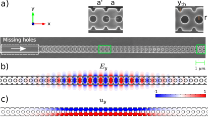
Figure 1: a) Scanning Electron Microscope image of the fabricated structure; the area where holes are removed is delimited by a dashed white line; white arrow: input light b) calculated normalized real part of the field $E_{y}$ for the fundamental optical mode at $\lambda$=1545 nm ; c) calculated normalized mechanical displacement $u_{y}$ at $f_{m}=3.12GHz$.

This design ensures the simultaneous localization of photons (Fig. 1b, $V_{opt}=0.97(\lambda/n)^{3}$) and phonons (Fig. 1c, $V_{m}=2.5\times 10^{-19}m^{3}$, $m_{eff}=1.01pg$). The cavity is coupled to the input waveguide by removing $n_{lh}$ holes and sidewall corrugation on one side (out of the 51 holes in total) and the waveguide is coupled to a lensed fiber using an inverse taper Tran et al. (2009).

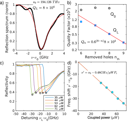
Figure 2: Fundamental mode: a) Reflection spectrum (black), Lorentzian fit (red) and extracted loaded Q factor for a cavity with 7 holes removed; b) measured loaded and intrinsic Q-factors as a function of the number of holes removed, and exponential fit (red line); c) normalized reflectivity as a function of the detuning; d) extracted thermo-optic shift as a function of the on-chip power $P_{c}$ for a cavity with 9 holes removed.

The device is fabricated on an InGaP membrane grown by MOCVD lattice-matched to GaAs. The OM crystal is processed following the same recipe as for two dimensional photonic crystalsCombrié et al. (2017, 2009).

Optical characterization

The optical resonances are probed in a reflection geometry using a high resolution optical heterodyne techniqueCombrié et al. (2017). This provides access to the complex spectrum of the cavity (see supplementary). Its modulus is shown in Fig. 2a. We consider the mode in the spectrum with the highest frequency (the fundamental). The loaded quality factor $Q_{L}$ decreases by a factor 0.6 for each period removed, while the intrinsic quality factor $Q_{0}$, extracted from the fit of the measured complex amplitude, is $2.2\pm 0.2\times 10^{5}$ (Fig. 2b).We measured an intrinsic quality factor over $10^{5}$ in 9 out of 12 nominally identical cavities. The whole spectrum is shown in Fig.9 of the supplementary information where the first order mode can be seen.
Absorption, at room temperature, is extracted from the normalized reflectivity as a function of the laser detuning $\nu_{L}-\nu_{0}$ swept from blue to red such that the resonance is thermally pulled Carmon et al. (2004) until the bistable transition occurs (Fig. 2c). This, to a very good approximation, corresponds to the detuned resonance $\nu^{\prime}$ (see supplementary information). When plotted against the on-chip power (i.e. the incident power), $\nu^{\prime}$ reveals a linear dependence (Fig. 2d), hence suggesting linear absorption, likely due to defects at the surface. Following the same procedure as in Martin et al. (2017), the dissipated power is extracted based on the calculated thermal resistance and the measured dependence of the resonance with temperature. This leads to an estimate of the absorption rate $\Gamma_{abs}/2\pi=8\,MHz$, which is much smaller than the total intrinsic losses $\Gamma_{0}/2\pi\approx 1GHz$. Correspondingly, the fraction of the dissipated on-chip power is $\alpha=4\Gamma_{abs}(\kappa-\Gamma_{0})/\kappa^{2}\approx 0.4\%$, with $\kappa$ the photon cavity decay rate. Absorption could be interpreted in terms of an effective imaginary refractive index through $n^{\prime}(InGaP)=n(InGaP)\Gamma_{abs}/2\pi\nu\approx 10^{-7}$, which is substantially lower than the estimate in Cole et al. (2014) at $\lambda=$1064nm and consistent with measurement of intrinsic $Q>10^{6}$ still limited by elastic scatteringCombrié et al. (2017).

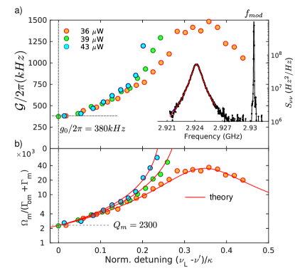
Figure 3: a) Measured vacuum optomechanical coupling as a function of the normalized laser detuning for 3 different on-chip laser power; inset : calibrated power spectral density of the frequency fluctuation along with calibration tone $f_{mod}$ and Lorentzian fit. b) corresponding measured mechanical linewidth compared to theory.

Probing of Brownian motion of the oscillator

The optomechanical crystal considered in this section* has an optical quality factor of $Q=3\times 10^{4}$. The noise spectrum of the mechanical resonator reveals several peaks. The one with the largest frequency ($f_{m}=2.924\ GHz$, see inset Fig3a) is identified as the fundamental mode (see Fig.10 of the supplementary for mechanical spectrum). The vacuum optomechanical coupling is measured at room temperature and standard pressure with the technique discussed in  Gorodetksy et al. (2010). The reflected optical power is detected by a fast Avalanche Photodiode which is amplified by a 40dB low noise amplifier before going to an electric spectrum analyser (ESA). The electric power spectra corresponding to the mechanical motion of the resonator is compared to a calibration tone with spectrum $S_{mod}$ generated by a phase modulator in the input optical path, allowing the measurement of the power spectrum of the frequency modulation $S_{\nu\nu}$, as shown in the inset of Fig. 3a (details in supplementary). In our case, it was not possible to operate the OM resonator at low enough power to avoid dynamical backaction while maintaining the detection level well above noise. Thus, what we measure and plot on Fig. 3a is a quantity $\mathcal{G}=\sqrt{\frac{\int{S_{\nu\nu}(f)df}}{n_{th}}}$ that corresponds to $g_{0}$ at vanishing laser-cavity detuning $\nu_{L}-\nu^{\prime}$, which is corrected for the thermally induced spectral shift, see supplementary. Considering the uncertainty on the photoelastic coefficients, the measured $g_{0}/2\pi=380$ kHz is very close to the calculations solely including the photoelastic and moving boundary contributions. This is consistent with the fact that the thermo-mechanical termGuha et al. (2017) is negligible in our system (discussion in Supplementary).
The corresponding mechanical linewidth (Fig. 3b) is measured and compared to theory Aspelmeyer et al. (2014) accounting for the narrowing due to the dynamical backaction $\Gamma_{om}$, when $\Delta=\nu_{L}-\nu^{\prime}>0$:

$$\Gamma_{om} =n_{h\nu}g_{0}^{2}\times$$

$$\times\left[\frac{\kappa}{(\Delta+2\pi f_{m})^{2}+\kappa^{2}/4}-\frac{\kappa}{\left(\Delta-2\pi f_{m}\right)^{2}+\kappa^{2}/4}\right]$$

with the number of photons in the cavity given by the usual coupled mode theory.

The parameters used in the model (gathered in a table in the supplementary) are measured: $\kappa/2\pi=6.5$ GHz, $\Gamma_{0}/2\pi=0.9$ GHz, $\Omega_{m}/2\pi=2.92$ GHz and $g_{0}/2\pi=380$ kHz. Only the on-chip laser power levels used in the model, $P_{c}=43.5$, $47.9$ and $51$ $\mu W$, have been adjusted within 20% of the experimental values indicated in Fig 3a. From the lorentzian fit in the inset of Fig 3a, the mechanical linewidth is equal to $\Gamma_{m}/2\pi=1.2MHz$ and the mechanical Q factor at room temperature and atmospheric pressure is $Q_{m}=\Omega_{m}/\Gamma_{m}=2300\pm 150$ corresponds to the measurement at zero detuning.

Self-sustained oscillations

We routinely observe self-sustained oscillations on devices with different loaded Q factor. We focus on the cavity with loaded quality factor $Q=30\ 000$. As the power is increased, the resonator eventually undergoes regenerative oscillations. The threshold is predicted by the condition that the mechanical loss equates the optical anti-damping calculated above: $\Gamma_{m}+\Gamma_{om}=0$. Using the measured parameters above yields $P_{c,tr}=47\mu W$, which is again, within 20% of the measured value, 40 $\mu W$.
The measurement is performed as the laser is swept towards the red across the resonance and repeated as the on-chip power is increased. Through the dynamical backaction, the mechanical mode drifts by 700 kHz for an on-chip power of $53\mu W$ (Fig. 4a). The mechanical linewidth is very well fitted by a Voigt function (Fig. 4b) which is the convolution of a gaussian function which Full Width at Half Maximum is equal to $\sigma_{G}=5047\pm 929Hz$ (which corresponds to the Resolution Bandwidth used to record the different spectra) and a lorentzian function. The lorentzian linewidth, corresponding to the short-term linewidth, decreases from $1.2\pm 0.08$ MHz to $\Gamma_{eff,L}/2\pi=80\pm 20Hz$ for an on-chip power of $53\mu W$.
On Fig. 4c), the short-term linewidth is plotted against the RF integrated power. We consider the transduction of the mechanical movement to the optical signal to be constant and linear. In that case, the number of phonons $\overline{n}$ can be deduced from $\overline{n}_{th}/\overline{n}=P_{RF,th}/P_{RF}$ where $\overline{n}_{th}$ is the number of phonons at thermal equilibrium, given by $\overline{n}_{th}=k_{B}T/\hbar\Omega_{m}$ and $P_{RF,th}$ is the RF integrated power at thermal equlibrium, when there is no dynamical backaction. The knowledge of the number of phonons allows one to calculate the limit to the short-term linewidth given in Vahala (2008); Hossein-Zadeh and Vahala (2010), similarly to the Shawlow-Townes limit for lasers:

$$\Gamma_{eff,L}=\Gamma_{m}\left(\frac{\overline{n}_{th}}{2\overline{n}}+\frac{1}{2\overline{n}}\right)\approx\Gamma_{m}\frac{\overline{n}_{th}}{2\overline{n}}$$ (1)

Eq 1 is valid above threshold and is plotted in black on Fig. 4c). As the measurements are performed at room temperature, $\overline{n}_{th}+1\approx\overline{n}_{th}$ and in that case, as pointed out in Ref.Hossein-Zadeh and Vahala (2010), the short-term linewidth is limited by thermal noise. As the experimental points obtained by fitting the spectra with the Voigt function follow the limit given by eq.1, we can conclude that the short-term linewidth of the self-sustained oscillations is limited by Brownian motion and this should be improved by lowering the temperature bath.

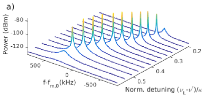
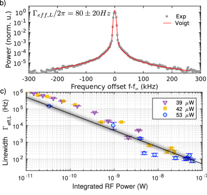
Figure 4: a) Raw spectra of the detected signal as a function of the detuning for $P_{c}=53\mu W$; b) Fit of normalized RF spectrum with the Voigt function; c) fitted Lorentzian linewidth $\Gamma{eff,L}$ as a function of the RF integrated power for different optical pump levels, the black line represents the estimated short term limit based on eq. 1, blur represents uncertainty on the measurement of the RF power at thermal equilibrium.

A deeper insight in the noise properties of the oscillatorHossein-Zadeh and Vahala (2010) is gained by examining the spectral density of the phase noise $\mathcal{L}(f)$ (Fig. 5), measured when the device is oscillating at its maximum amplitude. The cavity considered for this measurement has slightly different parameters (in particular a lower optical quality factor $Q=2.5\times 10^{4}$) and a stronger Signal to Noise Ratio is obtained through optical heterodyning (see supplementary). From 5kHz to 2 MHz the phase noise spectral power density follows the slope $PSD=\Gamma_{eff,L}/f^{2}$, which is associated to phase random walk. The Lorentzian linewidth $\Gamma_{eff,L}/2\pi=120Hz$ is extracted, which is consistent with the direct measurement on the signal spectral power (Fig. 4). While white phase noise, due to thermal noise in the photodetector, dominates at higher frequencies, technical noise ($1/f^{3}$) dominates below 5kHz, which is typical of a free running oscillator.

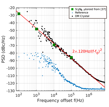
Figure 5: Measured phase noise spectrum (black filled circles), reference (blue filled circle), phase random walk noise corresponding to a Lorentzian linewidth $\Gamma_{eff,L}/2\pi=120Hz$ (red line) and corrected phase noise of the silicon nitride microtoroid from Tallur et al. (2011) (green squares)

Conclusion

In conclusion, an optomechanical crystal based on InGaP, a III-V piezoelectric semiconductor, has been developed based on a novel design involving only 4 parameters and requiring no optimization. The typical intrinsic optical Q factor is about $2\times 10^{5}$, whereas the loaded Q is controlled by removing holes. While nonlinear absorption is absent in the telecom spectral range, owing to the large electronic band-gap, the linear absorption is very small ($\Gamma_{abs}/2\pi=8MHz$), which, combined to a long thermal relaxation rate compared to the oscillation frequency, implies a negligible contribution of thermomechanical forces to damping $\Gamma_{om}$. The measured vacuum coupling constant is $g_{0}/2\pi\approx 380$ kHz, in good agreement with modeling. At room temperature and standard pressure, the mechanical damping is $Q_{m}=2300$, with a corresponding figure of merit $Q\times f=6\times 10^{12}$, which is of the same order of magnitude as Cole et al. (2014). Self-sustained oscillations are achieved routinely with a loaded optical $Q_{L}>2.5\times 10^{4}$, with an on-chip optical power level of about 40 $\mu W$. The measured mechanical short-term linewidth narrows down to about 100 Hz, limited by classical Brownian noise and would decrease with temperature. Compared to other optomechanical oscillators, the $1/f^{2}$ term of the phase noise is basically the same as in Silicon Nitride microtoroidsTallur et al. (2011), which is also a low loss material, once corrected for the carrier frequency to allow a fair comparison. We note that Micro-Electro-Mechanical Systems (MEMS) Sridaran and Bhave (2012) are about 10 dB below but our OMC provides an optical output, convenient for the distribution of the signal on-chip. Completed with piezo-electric transducers and hybridized on a Silicon Photonic circuit Tsvirkun et al. (2015), this device could be used for microwave to optical conversion and more elaborate miniaturized optoelectronic oscillators. We note that self-stabilisation schemes have been proposed for OM resonatorsMatsko et al. (2011). Further improvement could be achieved by inducing tensile stress in the membrane Bückle et al. (2018); Ghadimi et al. (2018). In perspective, this technology could be suitable for the investigation of complex non linear phenomena Navarro-Urrios et al. (2017), synchronization of several oscillators Heinrich et al. (2011) or quantum experiments.

Calculated parametric dependence of radiation losses, volume and OM coupling

.1 Dependence with hole radius

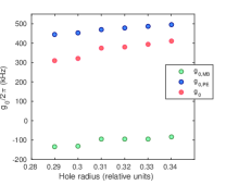
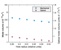
Figure 6: Evolution of the optomechanical coupling with the hole radius (units of a)

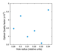
Figure 7: Evolution of the optical and mechanical volume with the hole radius (units of a)

Figure 8: Evolution of the optical quality factor with the hole radius (units of a)

The radius of the hole is a diffcult parameter to control during fabrication. The graph in Fig 8 show a variation of as much as 100 kHz for the optomechanical coupling with holes of increasing values.

.2 Dependence with teeth depth

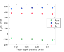
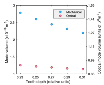
Figure 9: Evolution of the optomechanical coupling with teeth depth (units of a)

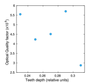
Figure 10: Evolution of the optical and mechanical volume with the teeth depth (units of a)

Figure 11: Evolution of the optical quality factor with the teeth depth (units of a)

As can be seen on Fig11, the depth of the teeth does not seem to have a significant influence on the optomechanical coupling $g_{0}$.
From figures 11 and 8, it can be seen that the optical quality factor does not depend on the hole radius and teeth depth when these paramters are changed over almost 30 nm, which suggests robustness against fabrication disorder.

Dependence with the ratio between the periods of the two lattices

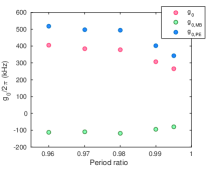
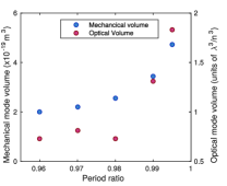
Figure 12: Evolution of the optomechanical coupling with the ratio of the periods (units of a)

Figure 13: Evolution of the optomechanical coupling with the ratio of the periods (units of a)

From Fig.13 and Fig.13, it is clear that as the ratio increases, the optical and the mechanical modes have a larger volume. Moreover, the optomechanical coupling $g_{0}$ is stronger when the mechanical and the optical modes are confined in a smaller volume.

Computing of vacuum OM coupling

The optomechanical coupling is calculated using the expressions from Balram et al. (2014) :

$$g_{0,MB} =-\frac{\omega_{0}}{2}\frac{\iint_{S}\overline{\overline{Q}}.\vec{n}\left(\Delta\varepsilon\left|\left|\vec{E}_{\parallel}\right|\right|^{2}-\Delta\varepsilon^{-1}\left|\left|\vec{D}_{\perp}\right|\right|^{2}\right)dS}{\iiint_{V}\varepsilon\left|\left|\vec{E}\right|\right|^{2}dV}$$ (2)

$$g_{0,PE} =\frac{\omega_{0}\varepsilon_{0}n^{4}}{2}\frac{\iiint_{V}\vec{E}\cdot p_{idkl}S_{kl}\cdot\vec{E}^{\ast}dV}{\iiint_{V}\varepsilon\left|\left|\vec{E}\right|\right|^{2}dV}$$ (3)

Photoelastic parameters

The photoelastic parameters for the computation of $g_{0}$ are taken from Mytsyk et al. (2015) :

$$p_{11} =-0.23$$

$$p_{12} =-0.13$$

$$p_{44} =-0.10$$

We note that there is an uncertainty of about $10\%$ on the above values. These values are given for a null angle with the (001) axis. As the injection axis of our cavities is along (110), a rotation must be applied to the photoelastic tensor.Balram et al. (2014).

Optical spectrum

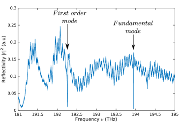
Figure 14: Optical spectrum of a cavity with $Q_{L}=120\ 000$ for the fundamental mode. The fundamental mode and the first order mode can be seen at respectively 194 THz and 192.25 THz

The spectrum on Fig.14 is recorded by Optical Coherence Tomography method Combrié et al. (2017). Two resonances can be seen on this spectrum : the resonance with the highest frequency (the fundamental mode) is around 194 THz and the next resonance (the first order mode) is around 192.25 THz. Interferences can also be seen in the reflection spectrum : the low frequency signature is attributed to the interference between the input of the waveguide and the fiber facet whereas the high frequency feature is linked to an interference between the input of the waveguide and the input of the photonic crystal. Further analysis of the reflection spectrum of such a cavity can be found in Lian et al. (2017).

Mechanical spectrum

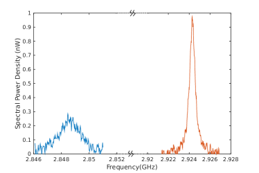
Figure 15: Mechanical spectrum of the bichromatic optomechanical crystal. The fundamental mode (orange) and the second order mode (blue) can be seen at respectively 2.92 GHz and 2.85 GHz

As can be seen on Fig.15, the fundamental mode at 2.92 GHz is indeed the mode with the highest mechanical frequency. The first order mode cannot be seen as it has an odd symmetry, whereas the fundamental optical mode has an even symmetry. According to calculation, $g_{0}$ between the fundamental optical mode and the second order mechanical mode is equal to $g_{0}/2\pi=23kHz$ which is much smaller than the $g_{0}/2\pi=380kHz$ for the coupling between the fundamental optical and mechanical modes.

Extraction of the Complex Amplitude Spectrum

The interferogram $s(\nu)$ which is measured with the OCT system is related to the complex amplitude of the optical field from the sample $\tilde{E}(\nu)=r(\nu)E_{r}$ through: $s=\tilde{E}E_{r}^{*}+c.c.=r\left|E_{r}\right|^{2}+c.c.$, where $E_{r}$ is the reference field. The transfer function (here the complex reflectivity) $r(\nu)$ can be retrieved using the Hilbert transform, as shown for instance in  Gottesman et al. (2004, 2010) to extract a complex spectrum from the time interferogram $r(t)$ measured by continuously changing the length of one of the arms of an unbalanced Michelson interferometer and a partially coherent light source. Here, the Hilbert transform is applied to a signal in the frequency domain, but the procedure is formally identical. This is achieved by taking the inverse Fourier transform $S$ of the interferogram $s$ and then calculating: $R(t)=S(t)+sign(t)S(t)$ and finally by Fourier transforming again to obtain $r(\nu)$.
From $r(\nu)$, the intrinsic losses $\Gamma_{0}$ and the coupling losses $\gamma$ can be deduced Combrié et al. (2017) :

$$r(\nu)=\frac{2\pi\nu-z}{2\pi\nu-p}$$ (4)

with $z$ and $p$ equal to :

$$z =2\pi\nu_{0}+i(\Gamma_{0}-\gamma)/2$$ (5)

$$p =2\pi\nu_{0}+i(\Gamma_{0}+\gamma)/2$$ (6)

Thermo Optic induced spectral shift

For a linear evolution of the resonance frequency with the on-chip power, the time-domain Coupled Mode Theory Fan et al. (2003) yields the following equation for the true value of the detuning :

$$\Delta^{\prime}=\Delta-\alpha P_{L}\frac{1}{1+\left[\frac{\Delta^{\prime}}{\kappa}\right]^{2}}$$ (7)

where $\Delta^{\prime}=2\pi(\nu_{L}-\nu_{0}^{\prime})$ and $\Delta=2\pi(\nu_{L}-\nu_{0})$, $\nu_{0}^{\prime}$ being the current resonance frequency and $\nu_{0}$ the ”cold” cavity resonance frequency.
From eq. (5) of Carmon et al. (2004), the maximum temperature change the system can undergo occurs when $\nu_{L}=\nu_{0}^{\prime}$ or equivalently, when $\Delta=\Delta\nu_{bist}$, $\Delta^{\prime}=0$ . Therefore, the true detuning can be written as a function of $\kappa$:

$$\Delta^{\prime}=\Delta-\frac{\Delta\nu_{bist}}{1+(4\pi\Delta^{\prime})^{2}/\kappa^{2}}$$ (8)

The above equation is therefore solved to obtain the real detuning.

Estimation of the on-chip power

Optical power is coupled into the photonic crystal cavity using a fiber-collimator and a microscope objective. When the pump is out of resonance, these two optical component are the main sources of losses. Therefore, the on-chip power is estimated by taking into account losses coming from the collimator and the objective :

$$P_{on-chip}=\alpha_{c}\alpha_{m}P_{input}$$ (9)

$$P_{reflected}=\alpha_{m}\alpha_{c}P_{on-chip}$$ (10)

where $\alpha_{c}$ corresponds to the loss due to the fiber-collimator and $\alpha_{m}$ represents the loss due to the microscope objective. Therefore, the on-chip power is found using the formula below :

$$P_{on-chip}=\sqrt{P_{reflected}P_{input}}$$ (11)

Measurement of the vacuum OM coupling

The optical source is a Keysight tuneable laser. The laser is then modulated by a MPZ LN 10 phase modulator from Photline Technologies. After coupling into the cavity, the reflected light is detected by an Optilab APR-10-M APD photodetector and analyzed by a Rhode and Schwarz FSV 40 Electrical Spectrum Analyser (ESA). The fiber link is entirely polarization maintaining.
The measurement of $g_{0}$ is carried out according to the method described in  Gorodetksy et al. (2010). The optomechanical coupling corresponds to the optical frequency shift resulting from the displacement of the mechanical resonator, therefore the method consist in measuring the power density spectrum of the frequency shift $S_{\nu\nu}(f)$ at thermal equilibrium, where the average amplitude of the thermal mechanical fluctuation is known and corresponds to $n_{th}=\frac{k_{B}T}{\hbar\Omega_{m}}$ phonons.
The vacuum coupling constant is therefore (by definition):

$$g_{0}^{2}=\frac{\int{S_{\nu\nu}(f)df}}{n_{th}}$$ (12)

where the integral is computed about the mechanical resonance $f_{m}$. The unknown transduction coefficient relating $S_{\nu\nu}$ to the measured electric power spectrum $S$ is determined using a calibration tone generated by phase modulator which is inserted in the input path between the light source and the cavity.

$$\int{S_{\nu\nu}(f)df}=\frac{\int{S(f)df}}{\int{S_{cal}(f)df}}\Phi_{0}^{2}\frac{(\pi f_{m})^{2}}{4}$$ (13)

where $S_{cal}$ is the spectral power density in the phase modulation peak and $\phi_{0}=\pi\frac{V_{cal}}{V_{\pi}}$, with $V_{\pi}=6.11$ V.
As the ESA measures the electrical power $\tilde{S}$ within the selected resolution bandwidth $RBW$, it follows that $\int{S_{cal}(f)df}=\tilde{S}_{cal}$ as the calibration tone is spectrally narrower than $RBW$. In contrast, the spectrum of the frequency fluctuations of the OM oscillator is broader and, following Gorodetksy et al. (2010), its integral is evaluated from the fitted Lorentzian lineshape with FWHM $\Gamma_{m}$ as: $\int{S(f)df}=\max(\tilde{S})\Gamma_{m}/RBW$. This leads to the known formula:

$$g_{0}^{2}=\frac{\max(\tilde{S})}{S_{cal}}\frac{\Gamma_{m}}{n_{th}}\phi_{0}^{2}\frac{\pi^{2}f_{m}^{2}}{4RBW}$$ (14)

The experiment is carried out by setting the calibration tone away from the resonance but still close enough such that the transduction function can still be considered constant.

Parameters used in the model

Optical properties	Coupled quality factor	$Q$	$30\ 000$
	Intrinsic quality factor	$Q_{0}$	$200\ 000$
	Resonance Frequency (THz)	$\nu_{0}$	$193.79$
Mechanical properties	Mechanical frequency(GHz)	$f_{m}$	$2.92$
	Quality factor	$Q_{m}$	2300
	Zero point fluctuation (fm)	$x_{ZPF}$	$1.6$
	Effective mass(fg)	$m_{eff}$	$1.07$
Thermal properties	Relaxation time $(\mu s)$	$\tau_{th}$	18
	Linear thermal expansion ($10^{-6}K$)	$\alpha$	5.3
	Thermomechanical force (nN)	$F_{th}$	$0.6$
Frequency shift per displacement ($Hz/m^{-1}$)		G	$1.51.10^{21}$
Optomechanical coupling ($kHz$)		$g_{0}$	$2\pi.385$

Influence of photothermal forces on anti-damping and optical spring

To quantify the influence of photothermal forces, we use the model developed in Guha et al. (2017), which takes into account the evolution of temperature in the OMC :

$$m_{eff}\ddot{x}+\Gamma_{m}m_{eff}\dot{x}+\omega_{m}^{2}x=\hbar G\left|a\right|^{2}+F_{th}$$ (15)

$$\dot{a}+\left(\frac{\kappa}{2}-i\Delta-iGx-\frac{\omega_{cav}}{n}\frac{dn}{dT}\right)a-\kappa_{ex}a_{in}=0$$ (16)

$$\frac{d\Delta T}{dt}=-\frac{\Delta T}{\tau_{th}}+\frac{\Gamma_{th}\left|a\right|^{2}}{\tau_{th}}$$ (17)

where $\Gamma_{th}=R_{th}\hbar\omega_{L}\kappa_{abs}$. $\tau_{th}$ is the thermal relaxation time, which is found by numerical simulation. $F_{th}$ is the photothermal force, found by considering the influence of a linear expansion of the OMC due to one photon absorbed. By linearizing around an equilibrium point, we find the expressions for the optical spring and anti-damping as a function of normalized detuning $x=\frac{\Delta}{\kappa}$ :

$$\begin{split}&\Gamma_{eff}=\frac{G}{m_{eff}\Omega\hbar\nu_{L}}\frac{\kappa_{ex}P}{\left[x^{2}+1/4\right]\kappa^{2}}\left[\frac{1}{2\kappa}\left[\hbar G+\frac{F_{th}}{1+(\Omega\tau_{th})^{2}}\right]\right.\\ &\left.\left[\frac{1}{1/4+(x+\Omega/\kappa)^{2}}-\frac{1}{1/4+(x-\Omega/\kappa)^{2}}\right]+\frac{F_{th}\Omega\tau_{th}}{1+(\Omega\tau_{th})^{2}}\right.\\ &\left.\left[\frac{x-\Omega/\kappa}{1/4+(x-\Omega/\kappa)^{2}}-\frac{x+\Omega/\kappa}{1/4+(x+\Omega/\kappa)^{2}}\right]\right]\end{split}$$ (18)

$$\begin{split}&\delta\Omega_{eff}=\frac{G}{m_{eff}\Omega}\frac{\kappa_{ex}P}{\left[x^{2}+1/4\right]\kappa^{2}}\frac{1}{\hbar\Omega_{L}}\left[\frac{1}{2\kappa}\left[\hbar G+\frac{F_{th}}{1+(\Omega\tau_{th})^{2}}\right]\right.\\ &\left[\frac{x+\Omega/\kappa}{1/4+(x+\Omega/\kappa)^{2}}+\frac{x-\Omega/\kappa}{1/4+(x-\Omega/\kappa)^{2}}\right]+\\ &\left.\frac{F_{th}\Omega\tau_{th}}{1+(\Omega\tau_{th})^{2}}\frac{1}{\kappa}\left[\frac{1/2}{1/4+(x-\Omega/\kappa)^{2}}-\frac{1/2}{1/4+(x+\Omega/\kappa)^{2}}\right]\right]\end{split}$$ (19)

From these equations, one can surmise that the influence of photothermal forces is negligible when the relaxation time is slow compared to the oscillation dynamics. Indeed, when plotting the contribution of photothermal forces to antidamping and comparing it to the antidamping due to radiation pressure (Fig 16), a difference of 4 orders of magnitude is clear between the two contributions.

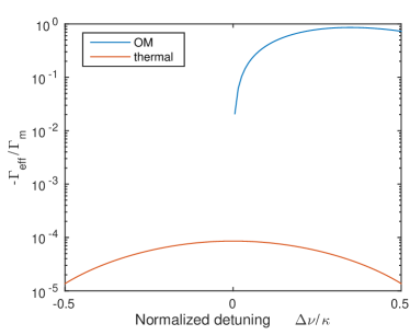
Figure 16: Comparison of the photothermal contribution and the contribution of the radiation pressure to antidamping as a function of normalized detuning

Measurement of the RF resonance

The RF spectra are fitted using the Voigt lineshape. This function is defined as the convolution of a Lorentzian lineshape $\mathcal{L}(x)=\gamma\pi^{-1}(x^{2}+\gamma^{2})^{-1}$ and a Gaussian broadening function $\mathcal{G}(x)=\exp(-x^{2}/2\sigma^{2})/\sqrt{2\pi}\sigma$, namely:

$$V(x;\gamma,\sigma)=\int{\mathcal{G}(x;\sigma)\mathcal{L}(x-x^{\prime};\gamma)dx^{\prime}}$$ (20)

The Voigt function is calculated efficiently through the Faddeeva function $w(z)$, (implemented in ), through the relations: $V(x;\gamma,\sigma)=\mathcal{R}[w(z)]/\sigma\sqrt{2\pi}$ and $z=(x+\imath\gamma)/\sigma\sqrt{2}$.

The fit is taken considering data points above the noise level estimated at -55 dB below the peak.
The integrated power is obtained by integrating the raw spectra $P_{RF}=\int{S}/RBW$, the resolution bandwidth, as above, unless the linewidth is narrower than the instrument resolution, where the peak level is taken instead.

Measurement of the phase noise

Phase noise is measured through the heterodyne technique Howe et al. (1981) using a Frequency Synthesizer as local oscillator at $f_{LO}$. First, the optical signal extracted from the cavity is mixed with a continuous wave strong optical carrier. The optical signal obtained after mixing is sent to a balanced photodetector (Discovery Semiconductors). The electrical signal is amplified using a 20 dB Mini Circuits amplifier then further amplified by another 40 dB (Femto Amplifier) before the mixer. The low frequency signal $v(t)$ is digitized with a 12bit real time sampling oscilloscope (Lecroy HDO), sampling time $1.25\times 10^{6}$ samples/s, with $N=2.5\times 10^{6}$ samples. Then, the signal $v_{n}=v(n\Delta t)$ is processed as in Maxin (2014) First $v_{n}$ is multiplied by $\exp(-2\pi\imath f_{0}\Delta tn)$ and Fourier transformed using FFT (denoted as $\mathcal{F})$. Then the low-frequency part of the spectrum ($|f|<BW$) is transformed back in the time domain, which gives the analytic signal $v_{a}$ around the carrier frequency $f_{0}=f_{OM}-f_{LO}$. The phase is obtained by taking the argument of each sample $\phi_{n}=arg(v_{a}(t_{n}))$. Then the power spectral density of the phase is evaluated within a certain spectral band $f\in[f_{i},f_{i+1}]$ using the standard procedure. This defines a time span $1/2f_{i}$ long enough to resolve $f_{i}$. Consequently $\phi_{n}$ is distributed in $N_{i}$ consecutive windows $\Delta W_{j}$ with duration $1/2f_{i}$ and containing $M_{i}$ samples, such that $M_{i}N_{i}=N$. In each time window, the non stationary contributions (trend and average) are removed and then a suitable window function (Hanning $h_{n}$) is applied to the signal $\tilde{\phi}_{n,j,i}$, before Fourier transform (FFT). Finally, the power spectra $S_{j,i}(f_{k,i})=|\mathcal{F}(\tilde{\phi}_{n,j,i}h_{n})|^{2}$ are averaged over the windows, being , $f_{k,i}\in[f_{i},f_{i+1}]$ . More precisely:

$$\mathcal{L}({f_{k,i})\approx\frac{\Delta t}{N_{i}M_{i}^{2}}\frac{\sum_{j=1}^{N_{i}}{S_{j,i}(f_{k,i})}}{\sum_{n}^{M_{i}}{h_{n}^{2}}}}$$ (21)

References

- Kippenberg and Vahala (2008) T. J. Kippenberg and K. J. Vahala, Science 321, 1172 (2008).
- Riedinger et al. (2018) R. Riedinger, A. Wallucks, I. Marinković, C. Löschnauer, M. Aspelmeyer, S. Hong, and S. Gröblacher, Nature 556, 473 (2018).
- Cohen et al. (2015) J. D. Cohen, S. M. Meenehan, G. S. MacCabe, S. Gröblacher, A. H. Safavi-Naeini, F. Marsili, M. D. Shaw, and O. Painter, Nature 520, 522 (2015).
- Purdy et al. (2017) T. P. Purdy, K. E. Grutter, K. Srinivasan, and J. M. Taylor, Science 356, 1265 (2017).
- Krause et al. (2012) A. G. Krause, M. Winger, T. D. Blasius, Q. Lin, and O. Painter, Nature Photonics 6, 768 (2012).
- Balram et al. (2016) K. C. Balram, M. I. Davanço, J. D. Song, and K. Srinivasan, Nature Photonics , 346 (2016).
- Massel et al. (2011) F. Massel, T. Heikkilä, J.-M. Pirkkalainen, S.-U. Cho, H. Saloniemi, P. J. Hakonen, and M. A. Sillanpää, Nature 480, 351 (2011).
- Hossein-Zadeh and Vahala (2010) M. Hossein-Zadeh and K. J. Vahala, IEEE Journal of Selected Topics in Quantum Electronics 16, 276 (2010).
- Eichenfield et al. (2009) M. Eichenfield, J. Chan, R. M. Camacho, K. J. Vahala, and O. Painter, Nature 462, 78 (2009).
- Enzian et al. (2019) G. Enzian, M. Szczykulska, J. Silver, L. D. Bino, S. Zhang, I. A. Walmsley, P. Del’Haye, and M. R. Vanner, Optica 6, 7 (2019).
- Davanço et al. (2014) M. Davanço, S. Ates, Y. Liu, and K. Srinivasan, Applied Physics Letters 104, 041101 (2014).
- Burek et al. (2016) M. J. Burek, J. D. Cohen, S. M. Meenehan, N. El-Sawah, C. Chia, T. Ruelle, S. Meesala, J. Rochman, H. A. Atikian, M. Markham, D. J. Twitchen, M. D. Lukin, O. Painter, and M. Lončar, Optica 3, 1404 (2016).
- Mitchell et al. (2016) M. Mitchell, B. Khanaliloo, D. P. Lake, T. Masuda, J. P. Hadden, and P. E. Barclay, Optica 3, 963 (2016).
- Midolo et al. (2018) L. Midolo, A. Schliesser, and A. Fiore, Nature nanotechnology 13, 11 (2018).
- Barzanjeh et al. (2015) S. Barzanjeh, S. Guha, C. Weedbrook, D. Vitali, J. H. Shapiro, and S. Pirandola, Phys. Rev. Lett. 114, 080503 (2015).
- Schneider et al. (2018) K. Schneider, Y. Baumgartner, S. Hönl, P. Welter, H. Hahn, D. J. Wilson, L. Czornomaz, and P. Seidler, arXiv:1812.00631 (2018).
- Mitchell et al. (2014) M. Mitchell, A. C. Hryciw, and P. E. Barclay, Applied Physics Letters 104, 141104 (2014).
- Bochmann et al. (2013) J. Bochmann, A. Vainsencher, D. D. Awschalom, and A. N. Cleland, Nature Physics 9, 712 (2013).
- Combrié et al. (2009) S. Combrié, Q. V. Tran, A. De Rossi, C. Husko, and P. Colman, Appl. Phys. Lett. 95, 221108 (2009).
- Colman et al. (2010) P. Colman, C. Husko, S. Combrié, I. Sagnes, C. W. Wong, and A. De Rossi, Nature Photonics 4, 862 (2010).
- Bückle et al. (2018) M. Bückle, V. C. Hauber, G. D. Cole, C. Gärtner, U. Zeimer, J. Grenzer, and E. M. Weig, Applied Physics Letters 113, 201903 (2018).
- Cole et al. (2014) G. D. Cole, P.-L. Yu, C. Gärtner, K. Siquans, R. Moghadas Nia, J. Schmöle, J. Hoelscher-Obermaier, T. P. Purdy, W. Wieczorek, C. A. Regal, and M. Aspelmeyer, Applied Physics Letters 104, 201908 (2014).
- Guha et al. (2017) B. Guha, S. Mariani, A. Lemaître, S. Combrié, G. Leo, and I. Favero, Optics Express 25, 24639 (2017).
- Combrié et al. (2017) S. Combrié, G. Lehoucq, G. Moille, A. Martin, and A. De Rossi, Laser and Photonics Reviews 11, 1700099 (2017).
- Dodane et al. (2018) D. Dodane, J. Bourderionnet, S. Combrié, and A. De Rossi, Optics Express 26, 20868 (2018).
- Safavi-Naeini et al. (2011) A. H. Safavi-Naeini, T. P. M. Alegre, J. Chan, M. Eichenfield, M. Winger, Q. Lin, J. T. Hill, D. E. Chang, and O. Painter, Nature 472, 69 (2011).
- Gomis-Bresco et al. (2014) J. Gomis-Bresco, D. Navarro-Urrios, M. Oudich, S. El-Jallal, A. Griol, D. Puerto, E. Chavez, Y. Pennec, B. Djafari-Rouhani, F. Alzina, et al., Nature Communications 5, 4452 (2014).
- (28) B.-S. Song, S. Noda, T. Asano, and Y. Akahane, Nature Materials 4, 207.
- Alpeggiani et al. (2015) F. Alpeggiani, L. C. Andreani, and D. Gerace, Applied Physics Letters 107, 261110 (2015).
- Baker et al. (2014) C. Baker, W. Hease, D.-T. Nguyen, A. Andronico, S. Ducci, G. Leo, and I. Favero, Opt. Express 22, 14072 (2014).
- Tran et al. (2009) Q. V. Tran, S. Combrié, P. Colman, and A. De Rossi, Appl. Phys. Lett. 95, 061105 (2009).
- Carmon et al. (2004) T. Carmon, L. Yang, and K. J. Vahala, Optics Express 12, 4742 (2004).
- Martin et al. (2017) A. Martin, D. Sanchez, S. Combrié, A. de Rossi, and F. Raineri, Opt. Lett. 42, 599 (2017).
- Gorodetksy et al. (2010) M. Gorodetksy, A. Schliesser, G. Anetsberger, S. Deleglise, and T. J. Kippenberg, Optics express 18, 23236 (2010).
- Aspelmeyer et al. (2014) M. Aspelmeyer, T. J. Kippenberg, and F. Marquardt, Reviews of Modern Physics 86, 1391 (2014).
- Vahala (2008) K. J. Vahala, Phys. Rev. A 78, 023832 (2008).
- Tallur et al. (2011) S. Tallur, S. Sridaran, and S. A. Bhave, Optics Express 19, 24522 (2011).
- Sridaran and Bhave (2012) S. Sridaran and S. A. Bhave, in 2012 IEEE 25th International Conference on Micro Electro Mechanical Systems (MEMS) (IEEE, 2012) pp. 664–667.
- Tsvirkun et al. (2015) V. Tsvirkun, A. Surrente, F. Raineri, G. Beaudoin, R. Raj, I. Sagnes, I. Robert-Philip, and R. Braive, Scientific Reports 5, 16526 (2015).
- Matsko et al. (2011) A. B. Matsko, A. A. Savchenkov, V. S. Ilchenko, D. Seidel, and L. Maleki, Phys. Rev. A 83, 021801(R) (2011).
- Ghadimi et al. (2018) A. H. Ghadimi, S. A. Fedorov, N. J. Engelsen, M. J. Bereyhi, R. Schilling, D. J. Wilson, and T. J. Kippenberg, Science 360, 764 (2018).
- Navarro-Urrios et al. (2017) D. Navarro-Urrios, N. E. Capuj, M. F. Colombano, P. D. Garcia, M. Sledzinska, F. Alzina, A. Griol, M. Alejandro, and C. M. Sotomayor-Torres, Nature Communications 8, 14965 (2017).
- Heinrich et al. (2011) G. Heinrich, M. Ludwig, J. Qian, B. Kubala, and F. Marquardt, Physical Review Letters 107, 043603 (2011).
- Balram et al. (2014) K. C. Balram, M. Davanço, J. Y. Lim, J. D. Song, and K. Srinivasan, Optica 1, 414 (2014).
- Mytsyk et al. (2015) B. G. Mytsyk, N. M. Demyanyshyn, and O. M. Sakharuk, Appl. Opt. 54, 8546 (2015).
- Lian et al. (2017) J. Lian, S. Sokolov, E. Yüce, S. Combrié, A. De Rossi, and A. P. Mosk, Phys. Rev. A 96, 033812 (2017).
- Gottesman et al. (2004) Y. Gottesman, E. Rao, and D. Rabus, J. Lightwave Tech. 22, 1566 (2004).
- Gottesman et al. (2010) Y. Gottesman, S. Combrié, A. DeRossi, A. Talneau, P. Hamel, A. Parini, R. Gabet, Y. Jaouen, B.-E. Benkelfat, and E. V. Rao, J. Lightwave Tech. 28, 816 (2010).
- Fan et al. (2003) . S. Fan, W. Suh, and J. Joannopoulos, J. Opt. Soc. Am. A 20, 569 (2003).
- Howe et al. (1981) A. Howe, D. W. Allan, and J. A. Barnes, Proc. 35th ann. symp. Freq. Control (1981).
- Maxin (2014) J. Maxin, Widely tunable optoelectronic oscillator and low noise for radar applications, Ph.D. thesis, Universite Toulouse III Paul Sabatier (2014).