PoS(LATTICE2018)119
ADP-18-32/T1080
DESY 18-220
Liverpool LTH 1190

The strange quark contribution to the spin of the nucleon

Abstract:

Quark line disconnected matrix elements of an operator, such as the axial current, are difficult to compute on the lattice. The standard method uses a stochastic estimator of the operator, which is generally very noisy. We discuss and develop further our alternative approach using the Feynman-Hellmann theorem which involves only evaluating two-point correlation functions. This is applied to computing the contribution of the quark spin to the nucleon and in particular for the strange quark. In this process we also pay particular attention to the development of an SU(3) flavour breaking expansion for singlet operators.

1 Introduction/Approach

The proton consists of two valence up quarks and one down quark together with a ‘sea’ of quark anti-quark pairs and gluons. How each constituent contributes to the total spin of the proton has remained a mystery for many years. In particular the quark contribution is much smaller than expected from the naive quark model. We discuss here our lattice QCD determination of the quark contribution, using a novel technique, based on a field theoretic application of the Feynman-Hellmann theorem, [1, 2].

There are two common spin decompositions or ‘schemes’: Jaffe–Manohar (JM), [3], and Ji, [4]. They both have a common quark spin term, $\Delta\Sigma/2$ but other pieces vary. In particular the JM approach has a gluon spin piece, $\Delta G$, which can be measured in $pp$ machines, while the Ji approach is more suitable for polarised DIS and DVCS processes and also lattice QCD determinations.

The Ji gauge invariant decomposition of the proton spin derived from the symmetric energy–momentum tensor is given by

$${1\over 2}={1\over 2}\Delta\Sigma_{p}+\sum_{q}L_{q}+J_{g}\,,$$ (1)

where $L_{q}$ is the orbital angular momentum of valence quark $q$ and $J_{g}$ is the gluon angular momentum. We shall not discuss these terms further here. The total quark spin $\Delta\Sigma_{p}=\Delta\Sigma^{\rm\scriptscriptstyle con}_{p}+\Delta\Sigma^{\rm\scriptscriptstyle dis}_{p}$ with

$$\Delta\Sigma^{\rm\scriptscriptstyle con}_{p}=\Delta u^{\rm\scriptscriptstyle con}_{p}+\Delta d^{\rm\scriptscriptstyle con}_{p}\,,\qquad\Delta\Sigma^{\rm\scriptscriptstyle dis}_{p}=\Delta u^{\rm\scriptscriptstyle dis}_{p}+\Delta d^{\rm\scriptscriptstyle dis}_{p}+\Delta s^{\rm\scriptscriptstyle dis}_{p}\,,$$ (2)

where $\Delta q^{\rm\scriptscriptstyle con,\,\rm\scriptscriptstyle dis}_{p}$ are the quark line connected and disconnected proton, $p$, matrix elements of the axial current respectively. We shall discuss the disconnected matrix elements further in the next section noting here that for the proton there is only a disconnected piece for the strange quark, so $\Delta s_{p}^{\rm\scriptscriptstyle dis}\equiv\Delta s_{p}$. Similar relations also hold for the other members of the baryon, $B$, nucleon octet.

The ‘Spin crisis’, discovered many years ago is that $\Delta\Sigma_{p}$ is small and only around $\sim 35\%$ of total spin, whereas in the naive quark model it would be expected that the valence quarks give the complete contribution $\Delta\Sigma_{p}\sim 1$. Here we shall consider $\Delta\Sigma^{\rm\scriptscriptstyle dis}_{B}$ and the $\Delta s^{\rm\scriptscriptstyle dis}_{B}$ pieces.

2 Feynman–Hellmann applied to field theories

If we modify the action by $S(\lambda)=S+\lambda O$, then it can be shown that [1]

$${\partial E_{B}(\lambda)\over\partial\lambda}={1\over 2E_{B}(\lambda)}\left\langle B\left|:\widehat{O}:\right|B\right\rangle_{\lambda}\,,$$ (3)

(where $:\ldots:$ means that the vacuum term has been subtracted.) Thus by suitably choosing $O$ and by identifying numerically the gradient of $E_{B}(\lambda)$ at $\lambda=0$ we can determine the desired matrix element. The computation requires only $2$-point correlation functions (rather than the more complicated $3$-point functions).

The modification location determines the contributions we access, as indicated in Fig. 1.

Figure 1: Left panel: Quark line connected $3$-point correlation functions; Right panel: Quark line disconnected $3$-point correlation functions.

We can modify the Dirac fermion matrix before quark propagator inversion

$$D^{\prime\,-1}=\left[D+\lambda O\right]^{-1}\quad\Rightarrow\quad\left.{\partial\over\partial\lambda}D^{\prime\,-1}\right|_{\lambda=0}=D^{-1}OD^{-1}\,,$$

which inserts connected contributions on the quark line or we can modify the field weighting during the HMC

$$\det D^{\prime}\,e^{-S_{g}}=\det[D+\lambda O]\,e^{-S_{g}}\quad\Rightarrow\quad\left.{\partial\over\partial\lambda}\det D^{\prime}\right|_{\lambda=0}=\mbox{tr}(D^{-1}O)\,\det D\,,$$ (4)

which acesses disconnected contributions. (Or do both modifications and obtain both connected and disconnected terms.) While the connected piece is easy to implement, the disconnected piece requires the generation of new configurations.

For a nucleon polarised in the $z$-direction we have

$$\langle B,\sigma|i\,\overline{q}\gamma_{3}\gamma_{5}q|B,\sigma\rangle=2M_{B}\sigma\Delta q\,\qquad\sigma=\pm\,,$$ (5)

which may be determined by applying the FH theorem to

$$C_{\sigma}(\lambda,t)\equiv(\Gamma_{\sigma})_{\beta\alpha}\langle B_{\alpha}(t)\overline{B}_{\beta}(0)\rangle_{\lambda}=A_{B}(\sigma\lambda)e^{-E_{B}(\sigma\lambda)}\,,$$ (6)

with corresponding projection operator $\Gamma_{\sigma}=\mbox{\small$\frac{1}{2}$}(1+\gamma_{4})(1+i\sigma\gamma_{3}\gamma_{5})$. As can be seen from eq. (5) flipping the sign of $\lambda$ is equivalent to flipping the spin polarisation, so we can write the amplitude and energy as a combined function of $\sigma\lambda$ . For the connected contributions this is sufficient, but a further complication arises for the disconnected terms, as for the generation of configurations using HMC the fermion matrix in the action must be $\gamma_{5}$-hermitian for HMC, i.e. we now need

$$S=S_{g}+\sum_{q\,x}\lambda_{q}\overline{q}(x)\gamma_{3}\gamma_{5}q(x)\,,$$ (7)

(rather than for the connected pieces, $D^{\prime}=D+i\sum_{q\,x}\lambda_{q}\overline{q}(x)\gamma_{3}\gamma_{5}q(x)$). The correlation function thus develops imaginary parts in both the amplitude $A_{B}(\sigma\lambda)\to A_{B}(\sigma\lambda)e^{i\delta(\sigma\lambda)}$, and energy $E_{B}(\sigma\lambda)\to E_{B}(\sigma\lambda)+i\phi(\sigma\lambda)$. Forming the ratio

$$R(\lambda,t)={{\rm Im}C_{+}(\lambda,t)-{\rm Im}C_{-}(-\lambda,t)\over{\rm Re}C_{+}(\lambda,t)-{\rm Re}C_{-}(-\lambda,t)}=-\tan(\phi(\lambda)t-\delta(\lambda))\,,$$ (8)

with effective phase shift

$$\phi(\lambda)={1\over t}\tan^{-1}\left(-R(\lambda,t)\right)\,,\qquad\mbox{where}\quad\phi(\lambda)=\phi_{0}\lambda+\phi_{1}\lambda^{3}+\ldots\,,$$ (9)

giving

$$\Delta q_{B}=\left.{\partial\phi(\lambda)\over\partial\lambda}\right|_{\lambda=0}\,.$$ (10)

This expression also holds for the connected piece and a test has been performed for the connected piece using the imaginary signal, to demonstrate its feasibility. (But of course it is better to use in this case the form where no imaginary piece develops.)

3 $SU(3)$ flavour symmetry breaking quark mass expansion

In [5] we developed $SU(3)$ flavour breaking expansions for hadron masses for $2+1$ flavours and extended it to matrix elements in [6]. We follow and extend the results given there (here just to ‘leading order’ or LO). The flavour structure is given from

$$A^{I}={1\over\sqrt{3}}\left(\bar{u}\gamma u+\bar{d}\gamma d+\bar{s}\gamma s\right)\,,\quad A^{\pi^{0}}={1\over\sqrt{2}}\left(\bar{u}\gamma u-\bar{d}\gamma d\right)\,,\quad A^{\eta}={1\over\sqrt{6}}\left(\bar{u}\gamma u+\bar{d}\gamma d-2\bar{s}\gamma s\right)$$ (11)

where $\gamma\sim\gamma_{i}\gamma_{5}$, $A$ for the axial current. So we can solve for $\bar{q}\gamma q\sim\Delta q$ in terms of $A^{I}$, $A^{\pi^{0}}$ and $A^{\eta}$. $SU(3)$ flavour breaking expansions for $A^{\pi^{0}}$, $A^{\eta}$, are given in [6]. In addition for the singlet operators, $A^{I}$ we need to consider $8\times 1\times 8$ tensors, which are similar to the mass expansions, [5].

We now consider the quark line ‘connected’ and ‘disconnected’ pieces separately and just give here the results for the disconnected part. (Complete expansions will be given in [7].) To LO we have for the $SU(3)$ flavour breaking expansion for $A^{I}$ for the baryon octet

$${1\over\sqrt{3}}\Delta\Sigma_{N}^{\rm\scriptscriptstyle dis} = a_{0}^{\rm\scriptscriptstyle dis}+3a_{1}^{\rm\scriptscriptstyle dis}\delta m_{l}$$

$${1\over\sqrt{3}}\Delta\Sigma_{\Sigma}^{\rm\scriptscriptstyle dis} = a_{0}^{\rm\scriptscriptstyle dis}-3a_{2}^{\rm\scriptscriptstyle dis}\delta m_{l}$$

$${1\over\sqrt{3}}\Delta\Sigma_{\Xi}^{\rm\scriptscriptstyle dis} = a_{0}^{\rm\scriptscriptstyle dis}-3(a_{1}^{\rm\scriptscriptstyle dis}-a_{2}^{\rm\scriptscriptstyle dis})\delta m_{l}\,,$$ (12)

together with $\Delta\Sigma_{\Lambda}^{\rm\scriptscriptstyle dis}/\sqrt{3}=a_{0}^{\rm\scriptscriptstyle dis}+3a_{2}^{\rm\scriptscriptstyle dis}\delta m_{l}$ and $\Delta\Sigma_{N_{s}}^{\rm\scriptscriptstyle dis}/\sqrt{3}=a_{0}^{\rm\scriptscriptstyle dis}-6a_{1}^{\rm\scriptscriptstyle dis}\delta m_{l}$, where $\Delta\Sigma_{B}^{\rm\scriptscriptstyle dis}=\Delta u_{B}^{\rm\scriptscriptstyle dis}+\Delta d_{B}^{\rm\scriptscriptstyle dis}+\Delta s_{B}^{\rm\scriptscriptstyle dis}$. All the expansions used here are for $2+1$ quark flavours, $m_{u}=m_{d}\equiv m_{l}$, $m_{s}$ and the ‘distance’ from the flavour symmetric point ($m_{l}=m_{s}$) is given by $\delta m_{l}=m_{l}-\overline{m}$, [5], where $\overline{m}$ is the average quark mass, held constant in simulations, so the expansion parameters remain constant. We have extended the nucleon octet to include a fictitious nucleon consisting of strange quarks, denoted by $N_{s}$. (As well as the $N$, $\Sigma$ and $\Xi$ this state can also be measured in a lattice simulation.) As we are primarily interested in the nucleon, and hence just $a_{1}^{\rm\scriptscriptstyle dis}$, it is convenient to consider the average of the $\Sigma$ and $\Xi$ expansions

$${1\over 2\sqrt{3}}(\Delta\Sigma_{\Sigma}^{\rm\scriptscriptstyle dis}+\Delta\Sigma_{\Xi}^{\rm\scriptscriptstyle dis})=a_{0}^{\rm\scriptscriptstyle dis}-{3\over 2}a_{1}^{\rm\scriptscriptstyle dis}\delta m_{l}\,.$$ (13)

Using the above results together with those for $A^{\pi^{0}}$ and $A^{\eta}$ gives the separate expansions of

$$\Delta s^{\rm\scriptscriptstyle dis}_{N} = {1\over\sqrt{3}}a_{0}^{\rm\scriptscriptstyle dis}+\left(\sqrt{3}a_{1}^{\rm\scriptscriptstyle dis}-{2\over\sqrt{6}}r_{1}^{\rm\scriptscriptstyle dis}\right)\delta m_{l}$$

$$\Delta s^{\rm\scriptscriptstyle dis}_{\Sigma} = {1\over\sqrt{3}}a_{0}^{\rm\scriptscriptstyle dis}+\left(-\sqrt{3}a_{2}^{\rm\scriptscriptstyle dis}-{2\over\sqrt{6}}r_{1}^{\rm\scriptscriptstyle dis}\right)\delta m_{l}$$

$$\Delta s^{\rm\scriptscriptstyle dis}_{\Xi} = {1\over\sqrt{3}}a_{0}^{\rm\scriptscriptstyle dis}+\left(-\sqrt{3}(a_{1}^{\rm\scriptscriptstyle dis}-a_{2}^{\rm\scriptscriptstyle dis})-{2\over\sqrt{6}}r_{1}^{\rm\scriptscriptstyle dis}\right)\delta m_{l}\,,$$ (14)

together with $\Delta s^{\rm\scriptscriptstyle dis}_{\Lambda}=a_{0}^{\rm\scriptscriptstyle dis}/\sqrt{3}+(\sqrt{3}a_{2}^{\rm\scriptscriptstyle dis}-2(r_{1}^{\rm\scriptscriptstyle dis}+2r_{2}^{\rm\scriptscriptstyle dis})/\sqrt{6})\delta m_{l}$, $\Delta s^{\rm\scriptscriptstyle dis}_{N_{s}}=a_{0}^{\rm\scriptscriptstyle dis}/\sqrt{3}+(-2\sqrt{3}a_{2}^{\rm\scriptscriptstyle dis}-2r_{1}^{\rm\scriptscriptstyle dis}/\sqrt{6})\delta m_{l}$. Due to isospin invariance we have $\Delta q_{p}^{\rm\scriptscriptstyle dis}=\Delta q_{n}^{\rm\scriptscriptstyle dis}\equiv\Delta q_{N}^{\rm\scriptscriptstyle dis}$, $\Delta q_{\Sigma^{+}}^{\rm\scriptscriptstyle dis}=\Delta q_{\Sigma^{-}}^{\rm\scriptscriptstyle dis}\equiv\Delta q_{\Sigma}^{\rm\scriptscriptstyle dis}$, $\Delta q_{\Xi^{0}}^{\rm\scriptscriptstyle dis}=\Delta q_{\Xi^{-}}^{\rm\scriptscriptstyle dis}\equiv\Delta q_{\Xi}^{\rm\scriptscriptstyle dis}$, for $q=u$, $d$, $s$. Note that due to constraints, the cancellation of the disconnected piece in $\Delta u_{N}^{\rm\scriptscriptstyle dis}-\Delta d_{N}^{\rm\scriptscriptstyle dis}$, $\Delta u_{\Sigma}^{\rm\scriptscriptstyle dis}-\Delta d_{\Sigma}^{\rm\scriptscriptstyle dis}$ and $\Delta u_{\Xi}^{\rm\scriptscriptstyle dis}-\Delta d_{\Xi}^{\rm\scriptscriptstyle dis}$ leads to the vanishing of $f^{\rm\scriptscriptstyle dis}$, $d^{\rm\scriptscriptstyle dis}$, $r_{3}^{\rm\scriptscriptstyle dis}$, $s_{1}^{\rm\scriptscriptstyle dis}$, $s_{2}^{\rm\scriptscriptstyle dis}$ in [6]. The results are more complicated for the ‘connected’ pieces; there are less constraints, [7].

Useful results are here to consider a ‘singlet of singlets’ and the strange quark terms alone

$$X_{\Delta\Sigma}^{\rm\scriptscriptstyle dis}\equiv{1\over 3}(\Delta\Sigma_{N}^{\rm\scriptscriptstyle dis}+\Delta\Sigma_{\Sigma}^{\rm\scriptscriptstyle dis}+\Delta\Sigma_{\Xi}^{\rm\scriptscriptstyle dis}) = \sqrt{3}a_{0}^{\rm\scriptscriptstyle dis}$$

$${1\over 3}\left(\Delta s_{N}^{\rm\scriptscriptstyle dis}+\Delta s_{\Sigma}^{\rm\scriptscriptstyle dis}+\Delta s_{\Xi}^{\rm\scriptscriptstyle dis}\right) = {1\over\sqrt{3}}a_{0}^{\rm\scriptscriptstyle dis}-\sqrt{2\over 3}r_{1}^{\rm\scriptscriptstyle dis}\delta m_{l}\,,$$ (15)

which together with eq. (13) allow separate determinations of $a_{0}^{\rm\scriptscriptstyle dis}$, $a_{1}^{\rm\scriptscriptstyle dis}$ and $r_{1}^{\rm\scriptscriptstyle dis}$.

4 Renormalisation

As the axial non-singlet currents $A^{\pi^{0}}$ and $A^{\eta}$ are (partially) conserved currents, they have no anomalous dimensions and so are scheme and scale independent. However the singlet current, $A^{I}$ is no longer conserved if $n_{f}\not=0$, as a topological term $\propto 2n_{f}(\alpha_{s}/4\pi)F_{\mu\nu}\widetilde{F}_{\mu\nu}$ appears in the Ward identity. Thus we expect the renormalisation constant to become scheme and scale dependent. It is also convenient to again consider the renormalisation of the quark line connected and disconnected pieces separately. We find [8, 9, 10]

$$\Delta q^{\rm\scriptscriptstyle con\,R}=Z_{A}\Delta q^{\rm\scriptscriptstyle con}\,,\qquad\Delta q^{\rm\scriptscriptstyle dis\,R}=Z_{A}\Delta q^{\rm\scriptscriptstyle dis}+{1\over 3}(Z_{A}^{\rm S}-Z_{A})(\Delta\Sigma^{\rm\scriptscriptstyle con}+\Delta\Sigma^{\rm\scriptscriptstyle dis})\,,$$ (16)

where $Z_{A}$ is the non-singlet renormalisation and $Z_{A}^{\rm S}$ is the singlet renormalisation factor. This gives

$$\Delta\Sigma^{\rm\scriptscriptstyle con\,\rm R}=Z_{A}\Delta\Sigma^{\rm\scriptscriptstyle con}\,,\qquad\Delta\Sigma^{\rm\scriptscriptstyle dis\,\rm R}=Z_{A}^{\rm S}\Delta\Sigma^{\rm\scriptscriptstyle dis}+(Z_{A}^{\rm S}-Z_{A})\Delta\Sigma^{\rm\scriptscriptstyle con}\,.$$ (17)

5 Results and Conclusions

We have a pion mass range from the flavour symmetric point $M_{\pi}\sim 460\,\mbox{MeV}$ down to $\sim 300\,\mbox{MeV}$ on $a\sim 0.074\,\mbox{fm}$, $32^{3}\times 64$ lattices and configurations as given in Table 1.

Data set $\#$	$\kappa_{l}$	$\kappa_{s}$	$\lambda_{l}$	$\lambda_{s}$
1	0.120900		-0.00625
2	0.120900		-0.0125 0
3	0.120900		0.0300
4	0.121095	0.120512	0.0000	0.0500
5	0.121095	0.120512	-0.0250
6	0.121095	0.120512	-0.0750

Table 1: Data sets used in the analysis.

We first consider $X_{\Delta\Sigma}^{\rm\scriptscriptstyle dis}$. In the left panel of Fig. 2 we show

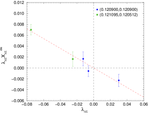
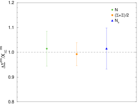
Figure 2: Left panel: $\phi_{\Delta\Sigma}=\lambda_{\Delta\Sigma}X_{\Delta\Sigma}^{\rm\scriptscriptstyle dis}$ together with a linear fit using data sets $1$–$3$ and $5$, $6$; Right panel: $\Delta\Sigma_{N}^{\rm\scriptscriptstyle dis}/X_{\Delta\Sigma}^{\rm\scriptscriptstyle dis}$, $(\Delta\Sigma_{\Sigma}^{\rm\scriptscriptstyle dis}+\Delta\Sigma_{\Xi}^{\rm\scriptscriptstyle dis})/(2X_{\Delta\Sigma}^{\rm\scriptscriptstyle dis})$ and $\Delta\Sigma_{N_{s}}^{\rm\scriptscriptstyle dis}/X_{\Delta\Sigma}^{\rm\scriptscriptstyle dis}$ for data set $6$.

$\phi_{\Delta\Sigma}=\lambda_{\Delta\Sigma}X_{\Delta\Sigma}$, from eq. (15) the gradient gives an estimation of $\sqrt{3}a_{0}^{\rm\scriptscriptstyle dis}$. Note that we can now use all the available data sets, $1$–$6$, to determine $X_{\Delta\Sigma}^{\rm\scriptscriptstyle dis}$ and hence $a_{0}^{\rm\scriptscriptstyle dis}$.

In the RH panel of Fig. 2 we show $\Delta\Sigma_{N}^{\rm\scriptscriptstyle dis}/X_{\Delta\Sigma}^{\rm\scriptscriptstyle dis}$, $(\Delta\Sigma_{\Sigma}^{\rm\scriptscriptstyle dis}+\Delta\Sigma_{\Xi}^{\rm\scriptscriptstyle dis})/(2X_{\Delta\Sigma}^{\rm\scriptscriptstyle dis})$ and $\Delta\Sigma_{N_{s}}^{\rm\scriptscriptstyle dis}/X_{\Delta\Sigma}^{\rm\scriptscriptstyle dis}$ for data set 6. From eqs. (12,13) we expect the numerical values of $1+3a_{1}^{\rm\scriptscriptstyle dis}/a_{0}^{\rm\scriptscriptstyle dis}\delta m_{l}$, $1+3/2a_{1}^{\rm\scriptscriptstyle dis}/a_{0}^{\rm\scriptscriptstyle dis}\delta m_{l}$ and $1-6a_{1}^{\rm\scriptscriptstyle dis}/a_{0}^{\rm\scriptscriptstyle dis}\delta m_{l}$ (where $\delta m_{l}\sim-0.07$) for $N$, $(\Sigma+\Xi)/2$ and $N_{s}$ respectively. We presently see very little pattern in the data, so presently we take $a_{1}^{\rm\scriptscriptstyle dis}\approx 0$. This indicates that this disconnected part is very small for all the baryons in the octet. A tentative general conclusion is that there is very little sign of $SU(3)$ flavour symmetry breaking effects in the disconnected pieces. Furthermore with $a_{1}^{\rm\scriptscriptstyle dis}\approx 0$ this also implies that

$$\Delta s_{N}^{\rm\scriptscriptstyle dis}\approx{1\over 3}\left(\Delta s_{N}^{\rm\scriptscriptstyle dis}+\Delta s_{\Sigma}^{\rm\scriptscriptstyle dis}+\Delta s_{\Xi}^{\rm\scriptscriptstyle dis}\right)\,,$$ (18)

also away from the $SU(3)$ flavour symmetry point. So when using data set 4 we can avoid a direct determination of $r_{1}^{\rm\scriptscriptstyle dis}$.

We have computed $Z_{A}$ and $Z_{A}^{\rm S}$ at $2\,\mbox{GeV}$ in [11], also using the FH method to give $Z_{A}=0.8458(8)$, $Z_{A}^{\rm S}(2\,\mbox{GeV})=0.8662(34)$ (the latter in the $\overline{MS}$ scheme). Note that this means that, as expected $(Z_{A}^{\rm S}-Z_{A})/Z_{A}^{\rm S}\sim 2\%$ a small difference, which we shall presently ignore. In Fig. 3 we show the renormalised results for $\Delta s_{N}$ in the $\overline{MS}$ scheme at a scale of $2\,\mbox{GeV}$.

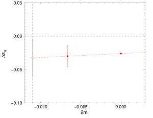
Figure 3: $\Delta s_{N}$ in the $\overline{MS}$ scheme at a scale of $2\,\mbox{GeV}$ versus $\delta m_{l}$. The vertical line indicates where the physical pion mass lies, [12].

Linearly extrapolating to the physical pion mass we find a preliminary result of $\Delta s_{N}(2\,\mbox{GeV})=-0.032(26)$.

In conclusion ‘disconnected’ quantities are notoriously difficult quantities to compute as they are a short distance quantity and suffers from large fluctuations. As alternative to more standard ‘stochastic’ approaches we have developed a method using the Feynman–Hellmann theorem, together with a $SU(3)$ flavour breaking expansion.

References

- [1] A. J. Chambers et al., [QCDSF–UKQCD–CSSM Collaborations], Phys. Rev. D90 (2014) 014510, [arXiv:1405.3019[hep-lat]].
- [2] A. J. Chambers et al., [QCDSF–UKQCD–CSSM Collaborations], Phys. Rev. D92 (2015) 114517, [arXiv:508.06856[hep-lat]].
- [3] R. L. Jaffe et al., Nucl. Phys. B337 (1990) 509.
- [4] X.-D. Ji, Phys. Rev. Lett. 78 (1997) 610, [arXiv:hep-ph/9603249].
- [5] W. Bietenholz et al., [QCDSF–UKQCD Collaborations], Phys. Rev. D84 (2011) 054509, [arXiv:1102.5300[hep-lat]].
- [6] A. N. Cooke et al., [QCDSF–UKQCD Collaborations], PoS(Lattice 2012) 116, arXiv:1212.2564[hep-lat].
- [7] QCDSF Collaboration, in preparation.
- [8] G. S. Bali et al., [QCDSF Collaboration], Phys. Rev. Lett. 108 (2012) 222001, [arXiv:1112.3354[hep-lat]].
- [9] J. Green et al., Phys. Rev. D95 (2017) 114502, [arXiv:1703.06703[hep-lat]].
- [10] J. Liang et al., [QCD Collaboration], Phys. Rev. D98 (2018) 074505, [arXiv:1806.08366[hep-lat]].
- [11] A. J. Chambers et al., [QCDSF Collaboration], Phys. Lett. B740 (2015) 30, [arXiv:1410.3078[hep-lat]].
- [12] R. Horsley et al., [QCDSF–UKQCD Collaborations], Phys. Rev. D91 (2015) 074512, arXiv:1411.7665[hep-lat].