Mixed Variational Inference

Abstract

The Laplace approximation has been one of the workhorses of Bayesian inference. It often delivers good approximations in practice despite the fact that it does not strictly take into account where the volume of posterior density lies. Variational approaches avoid this issue by explicitly minimising the Kullback-Leibler divergence D_KL between a postulated posterior and the true (unnormalised) logarithmic posterior. However, they rely on a closed form D_KL in order to update the variational parameters. To address this, stochastic versions of variational inference have been devised that approximate the intractable D_KL with a Monte Carlo average. This approximation allows calculating gradients with respect to the variational parameters. However, variational methods often postulate a factorised Gaussian approximating posterior. In doing so, they sacrifice a-posteriori correlations. In this work, we propose a method that combines the Laplace approximation with the variational approach. The advantages are that we maintain: applicability on non-conjugate models, posterior correlations and a reduced number of free variational parameters. Numerical experiments demonstrate improvement over the Laplace approximation and variational inference with factorised Gaussian posteriors.

I Introduction

Bayesian inference provides a way of making use of the complete information available either as data or prior knowledge. It enables us to capture the uncertainty present in the data and model assumptions, and propagate it to further tasks such as prediction and decision making. However, exact Bayesian inference is only possible whenever mathematically convenient priors are combined with particular likelihood functions (e.g. conjugacy). Deviation from such convenience, results in intractable calculations that call for approximations.

The Laplace approximation (LA) has helped the advancement of Bayesian methodology in the machine learning field [1] and has also been an important tool for practitioners [2]. LA produces a Gaussian approximating posterior. In doing so, it operates myopically in the sense that it determines the mean and covariance simply by looking locally around the mode instead of focusing on where the volume of the density actually lies. Despite this shortcoming, it has been found to produce good approximations in a variety of contexts. In a Gaussian process binary classification setting [3], LA is found to be on a par with other approximations in terms of error rate, though it performed poorer on other criteria. The work in [4] employs LA in order to calculate approximate intractable integrals within the Expectation Propagation algorithm [5]. In [6] LA is found to perform well when compared to Expectation Propagation in a bounded regression task. In [7] LA is used to formulate an approximate form of the marginal likelihood that facilitates the update of hyperparameters without the need to update the current Gaussian posterior given by LA.

Variational inference has been put forward (VI) [8, 9] as a solution to calculating posterior distributions in situations where certain expectations are not analytically tractable. Its use has been widespread in eliciting posterior densities in e.g. dimensionality reduction [10], classification [11], regression [9], density estimation [12] and in specialised applications like in astronomy [13]. The applicability of VI depends on choosing a posterior density form that allows the Kullback-Leibler divergence ($\operatorname{D\textsubscript{KL}}$) between the approximating and the true (unnormalised) posterior to be calculated in closed form. However, such a choice may not always exist.

Whenever it is not possible to obtain a closed-form $\operatorname{D\textsubscript{KL}}$ within the VI framework, approximations become necessary. One type of approximation approximates the logarithmic (unnormalised) posterior. In [14] the logarithmic posterior is linearised via a first-order Taylor expansion which allows then calculating the expectation with respect to the approximating posterior in the $\operatorname{D\textsubscript{KL}}$. In a similar vein, second order Taylor expansions are considered in [15]. Interestingly, [16] considers multiple second order Taylor expansions at different parameter locations of the logarithmic posterior. This results in an approximate posterior density expressed as a mixture of spherical Gaussians that has the potential to capture multiple modes. A second type of approximation [17, 18, 19, 20] approximates the $\operatorname{D\textsubscript{KL}}$ as a Monte Carlo average with samples drawn from the approximating posterior. The resulting expression allows calculating the gradient with respect to the free variational parameters. An update of the variational parameters follows, typically using a small step size in a stochastic gradient descent setting, after which the $\operatorname{D\textsubscript{KL}}$ is approximated with a new Monte Carlo average. In a slightly manner, [21, 22] fix the Monte Carlo average approximation of the $\operatorname{D\textsubscript{KL}}$ throughout the optimisation of the variational parameters. We finally note that often in practice e.g. [17, 19], VI methods choose to work with a factorised Gaussian posterior which has the advantage of reducing the number of free variational parameters that need to be optimised, but also has the inevitable disadvantage of discarding potential parameter correlations in the posterior.

In this work, we propose a method that combines the Laplace approximation with the variational approximation. The method works on non-conjugate models, captures a-posteriori correlations and limits the number of free variational parameters. The main idea is to take the Gaussian posterior obtained from the Laplace approximation, plug it into the variational lower bound and adapt it by optimising the lower bound. The crux of the approach is to allow only a partial update of the Laplace Gaussian posterior.

II Approximate Bayesian Inference

We briefly review methods for approximate inference as a gentle reminder and for the purpose of introducing relevant notation. We write the log-posterior as the sum of the model log-likelihood, log-prior and minus log-evidence:

$$\ln p(\mbox{\boldmath$w$}|\mbox{\boldmath$\theta$},\mathcal{D})=\ln p(\mathcal{D}|\mbox{\boldmath$w$},\mbox{\boldmath$\theta$}_{\ell})+\ln p(\mbox{\boldmath$w$}|\mbox{\boldmath$\theta$}_{\pi})-\ln\mathcal{Z}\ ,$$ (1)

where $\mathcal{D}$ are the data, $\mbox{\boldmath$w$}\in\mathbb{R}^{D}$ are the model parameters and $\mathcal{Z}=\int p(\mathcal{D}|\mbox{\boldmath$w$},\mbox{\boldmath$\theta$}_{\ell})p(\mbox{\boldmath$w$}|\mbox{\boldmath$\theta$}_{\pi})\mbox{\boldmath$dw$}$. The log-likelihood and log-prior terms have hyperparameters $\mbox{\boldmath$\theta$}_{\ell}$ and $\mbox{\boldmath$\theta$}_{\pi}$ which are jointly summarised as $\theta$ in the log-posterior. In the following, the evidence is a constant which we discard. Discarding it, gives us the unnormalised log-posterior $\ln\tilde{p}(\mbox{\boldmath$w$}|\mbox{\boldmath$\theta$},\mathcal{D})$.

II-A Laplace approximation

The Laplace approximation (LA) seeks the mode $\mbox{\boldmath$w$}^{*}$ of the log-posterior density $\ln\tilde{p}(\mbox{\boldmath$w$}|\mbox{\boldmath$\theta$},\mathcal{D})$ where $\mbox{\boldmath$0$}=\nabla_{\tiny\mbox{\boldmath$w$}}\ln\tilde{p}(\mbox{\boldmath$w$}|\mbox{\boldmath$\theta$},\mathcal{D})|_{\scriptstyle\mbox{\boldmath$\scriptstyle w$}=\mbox{\boldmath$\scriptstyle w$}^{*}}$. This may be carried out with gradient-based optimisation. At the found mode, we calculate the Hessian matrix $\mbox{\boldmath$H$}=\nabla\nabla\ln\tilde{p}(\mbox{\boldmath$w$}|\mbox{\boldmath$\theta$},\mathcal{D})|_{\scriptstyle\mbox{\boldmath$\scriptstyle w$}=\mbox{\boldmath$\scriptstyle w$}^{*}}$. The obtained approximating Gaussian posterior reads:

$$q(\mbox{\boldmath$w$})=\mathcal{N}(\mbox{\boldmath$w$}|\mbox{\boldmath$\mu$}_{LA}=\mbox{\boldmath$w$}^{*},\mbox{\boldmath$\Sigma$}_{LA}=-\mbox{\boldmath$H$}^{-1})\ .$$ (2)

We see that the covariance of the approximating posterior $q(\mbox{\boldmath$w$})$ is given by the local curvature of the posterior at the found mode. The approximation can be good, if the true posterior concentrates strongly around the mode.

II-B Variational Inference

Variational inference (VI) [8] postulates an approximating posterior $q(\mbox{\boldmath$w$})$. VI finds the $q(\mbox{\boldmath$w$})$ that maximises the following $\operatorname{D\textsubscript{KL}}$ based objective, also known as the variational lower bound [23, Chapter $10$] :

$$-\operatorname{D\textsubscript{KL}}(q(\mbox{\boldmath$w$})||\tilde{p}(\mbox{\boldmath$w$}|\mbox{\boldmath$\theta$},\mathcal{D})) =\int q(\mbox{\boldmath$w$})\ln\tilde{p}(\mbox{\boldmath$w$}|\mbox{\boldmath$\theta$},\mathcal{D})\mbox{\boldmath$dw$}$$

$$\ \ \ \ -\int q(\mbox{\boldmath$w$})\ln q(\mbox{\boldmath$w$})\mbox{\boldmath$dw$}\ .$$ (3)

In general, VI does not require that $q(\mbox{\boldmath$w$})$ is a Gaussian, but here we choose to work with $q(\mbox{\boldmath$w$})=\mathcal{N}(\mbox{\boldmath$w$}|\mbox{\boldmath$\mu$},\mbox{\boldmath$\Sigma$})$. For this choice, the above objective now reads as:

$$\int\mathcal{N}(\mbox{\boldmath$w$}|\mbox{\boldmath$\mu$},\mbox{\boldmath$\Sigma$})\ln\tilde{p}(\mbox{\boldmath$w$}|\mbox{\boldmath$\theta$},\mathcal{D})\mbox{\boldmath$dw$}+\frac{1}{2}\ln|2\pi e\mbox{\boldmath$\Sigma$}|\ ,$$ (4)

where the second term is the Gaussian entropy. The free parameters in objective (4) are the variational parameters $\mu$, $\Sigma$ and hyperparameters $\theta$.

II-C Stochastic variational inference

Stochastic variational inference [19] addresses the difficulty that arises when the expectation in the first term of (4) is not tractable. It does so by approximating the expectation by a Monte Carlo average with samples drawn from $\mbox{\boldmath$w$}_{s}\sim q(\mbox{\boldmath$w$})$:

$$\frac{1}{S}\sum_{s=1}^{S}\ln\tilde{p}(\mbox{\boldmath$w$}_{s}|\mbox{\boldmath$\theta$},\mathcal{D})+\frac{1}{2}\ln|2\pi e\mbox{\boldmath$\Sigma$}|\ .$$ (5)

The variational parameters no longer appear in the approximation, but it is possible to reintroduce them using the reparametrisation $\mbox{\boldmath$w$}_{s}=\mbox{\boldmath$\mu$}+\mbox{\boldmath$C$}\mbox{\boldmath$z$}_{s}$, in terms of samples $\mbox{\boldmath$z$}_{s}\sim\mathcal{N}(\mbox{\boldmath$0$},\mbox{\boldmath$I$}_{D})$:

$$\frac{1}{S}\sum_{s=1}^{S}\ln\tilde{p}(\mbox{\boldmath$\mu$}+\mbox{\boldmath$C$}\mbox{\boldmath$z$}_{s}|\mbox{\boldmath$\theta$},\mathcal{D})+\frac{1}{2}\ln|2\pi e\mbox{\boldmath$\Sigma$}|\ ,$$ (6)

where $C$ is a matrix such that $\mbox{\boldmath$C$}\mbox{\boldmath$C$}^{T}=\mbox{\boldmath$\Sigma$}$. The free parameters in objective (6) are $\mu$, $\Sigma$ and $\theta$. We note that, typically, one chooses covariance $\Sigma$ to be a diagonal matrix (e.g. [17, 19]) in order to limit the number of free variational parameters to be optimised. In this case, $q(\mbox{\boldmath$w$})$ is a factorised posterior.

III Proposed method

The motivation behind this work is to apply VI on non-conjugate models using an approximating posterior $q(\mbox{\boldmath$w$})$ that captures a-posteriori correlations but at the same time limits the number of free variational parameters that need to be optimised. To that end, we make use of the covariance $\mbox{\boldmath$\Sigma$}_{LA}$ of the approximating posterior $q(\mbox{\boldmath$w$})$ obtained via LA and the approximate variational lower bound in (6). Since the proposed method combines LA with the variational lower bound, we name it mixed variational inference (MVI). In the following, we propose three ways that MVI can exploit the correlation structure present in $\mbox{\boldmath$\Sigma$}_{LA}$.

III-A Adaptation of mean only - MVI_$\mu$

We perform the following Cholesky decomposition:

$$\mbox{\boldmath$\Sigma$}_{LA}=\mbox{\boldmath$C$}_{LA}\mbox{\boldmath$C$}_{LA}^{T}\ .$$ (7)

We propose the posterior $q(\mbox{\boldmath$w$})=\mathcal{N}(\mbox{\boldmath$w$}|\mbox{\boldmath$\mu$},\mbox{\boldmath$\Sigma$}_{LA})$ and use it in the approximate variational lower bound in (6), which results in the following objective:

$$\frac{1}{S}\sum_{s=1}^{S}\ln\tilde{p}(\mbox{\boldmath$\mu$}+\mbox{\boldmath$C$}_{LA}\mbox{\boldmath$z$}_{s}|\mbox{\boldmath$\theta$},\mathcal{D})+\frac{1}{2}\ln|2\pi e\mbox{\boldmath$\Sigma$}_{LA}|\ ,$$ (8)

The free parameters in (8) are the mean $\mu$ and hyperparameters $\theta$. Effectively, the proposed posterior is the Laplace posterior with the added flexibility of shifting its mean while keeping its covariance fixed to $\mbox{\boldmath$\Sigma$}_{LA}$. Note, that here the entropy is a constant term that can be discarded during optimisation.

III-B Mean and scaling of covariance - MVI_eig

We perform the following eigenvalue decomposition:

$$\mbox{\boldmath$\Sigma$}_{LA}=\mbox{\boldmath$Q$}_{LA}\operatorname{diag}(\mbox{\boldmath$r$}_{LA}^{2})\mbox{\boldmath$Q$}_{LA}^{T}\ ,$$ (9)

where matrix $\mbox{\boldmath$Q$}_{LA}\in\mathbb{R}^{D\times D}$ and vector $\mbox{\boldmath$r$}_{LA}\in\mathbb{R}^{D}$ hold the eigenvectors and square roots of the eigenvalues respectively. We propose $q(\mbox{\boldmath$w$})=\mathcal{N}(\mbox{\boldmath$w$}|\mbox{\boldmath$\mu$},\mbox{\boldmath$Q$}_{LA}\operatorname{diag}(\mbox{\boldmath$r$}^{2})\mbox{\boldmath$Q$}_{LA}^{T})$ and optimise:

$$\frac{1}{S}\sum_{s=1}^{S}\ln\tilde{p}(\mbox{\boldmath$\mu$}+\mbox{\boldmath$Q$}_{LA}\operatorname{diag}(\mbox{\boldmath$r$})\mbox{\boldmath$z$}_{s}|\mbox{\boldmath$\theta$},\mathcal{D})+\frac{1}{2}\ln|2\pi e\operatorname{diag}(\mbox{\boldmath$r$}^{2})|\ .$$ (10)

The free parameters in (10) are $\mu$, $r$ and $\theta$. Note the simplification in the entropy term due to the orthogonal $\mbox{\boldmath$Q$}_{LA}$, i.e. $|2\pi e\operatorname{diag}(\mbox{\boldmath$r$}^{2})\mbox{\boldmath$Q$}_{LA}^{T}\mbox{\boldmath$Q$}_{LA}|=|2\pi e\operatorname{diag}(\mbox{\boldmath$r$}^{2})|$. Effectively, the proposed posterior is the Laplace posterior which now has the added flexibility to shift the mean and scale the covariance matrix along its axes by adapting vector $r$.

III-C Mean and low rank update of covariance - MVI_lr

We introduce the vectors $\mbox{\boldmath$U$},\mbox{\boldmath$V$}\in\mathbb{R}^{D}$. We use the Cholesky decomposition $\mbox{\boldmath$\Sigma$}_{LA}=\mbox{\boldmath$C$}_{LA}\mbox{\boldmath$C$}_{LA}^{T}$ and form the matrix $\mbox{\boldmath$L$}=\mbox{\boldmath$C$}_{LA}+\mbox{\boldmath$U$}\mbox{\boldmath$V$}^{T}$. We propose the posterior $q(\mbox{\boldmath$w$})=\mathcal{N}(\mbox{\boldmath$w$}|\mbox{\boldmath$\mu$},\mbox{\boldmath$L$}\mbox{\boldmath$L$}^{T})$ and the associated objective:

$$\frac{1}{S}\sum_{s=1}^{S}\ln\tilde{p}(\mbox{\boldmath$\mu$}+\mbox{\boldmath$L$}\mbox{\boldmath$z$}_{s}|\mbox{\boldmath$\theta$},\mathcal{D})+\frac{1}{2}\ln|2\pi e\mbox{\boldmath$L$}\mbox{\boldmath$L$}^{T}|\ .$$ (11)

The free parameters in (11) are $\mu$, $U$, $V$ and $\theta$. Effectively, the proposed posterior is the Laplace posterior which now has the added flexibility to shift the mean but also modify its covariance matrix via a low-rank update.

The proposed posteriors are summarised in Table I.

III-D Initialisation

We use the mean $\mbox{\boldmath$\mu$}_{LA}$ and optimised hyperparameters $\mbox{\boldmath$\theta$}_{LA}$ obtained from the Laplace approximation to initialise the mean in $q(\mbox{\boldmath$w$})=\mathcal{N}(\mbox{\boldmath$w$}|\mbox{\boldmath$\mu$}=\mbox{\boldmath$\mu$}_{LA},\mbox{\boldmath$\Sigma$})$ and hyperparameters $\mbox{\boldmath$\theta$}=\mbox{\boldmath$\theta$}_{LA}$ in each of the three proposed objectives. We emphasize that the covariance in MVI_$\mu$ is initialised to $\mbox{\boldmath$\Sigma$}_{LA}$ and fixed. Vector $r$ in MVI_eig is initialised to the square root of the eigenvalues $\mbox{\boldmath$r$}_{LA}$. Vectors $U$,$V$ in MVI_lr are randomly initialised by drawing them from $\mathcal{N}(\mbox{\boldmath$0$},0.01\mbox{\boldmath$I$}_{D})$.

III-E Optimisation

TABLE I: Summary of MVI posteriors. Variables with the subscript LA are fixed parameters (not optimised) whose values are given by either the Cholesky or eigenvalue decomposition.

	MVI$\mu$	MVIeig	MVIlr
# parameters	D	2D	3D
mean	$\mu$	$\mu$	$\mu$
covariance “root”	$\mbox{\boldmath$C$}_{LA}$	$\mbox{\boldmath$Q$}_{LA}\operatorname{diag}(\mbox{\boldmath$r$})$	$\mbox{\boldmath$C$}_{LA}+\mbox{\boldmath$U$}\mbox{\boldmath$V$}^{T}$

Following [21, 22] we draw $S$ number of samples $\mbox{\boldmath$z$}_{s}\sim\mathcal{N}(\mbox{\boldmath$0$},\mbox{\boldmath$I$}_{D})$ which we keep fixed throughout the optimisation of the objectives in (8), (10) and (11). This enables the use of scaled-conjugate gradients (SCG) as the optimisation routine[24] in contrast to the typically employed stochastic gradient descent [19]. We note that the proposed method can in principle also employ the same optimisation scheme as in [19]. The free parameters $\mu$, $\theta$ and the ones pertaining to the covariance in each proposed posterior are jointly optimised via SCG. In all experiments we fix the number of drawn samples $\mbox{\boldmath$z$}_{s}$ to $S=10^{3}$.

IV Numerical setup

IV-A Comparisons

The proposed work builds on LA and VI in order to improve the performance (see section IV-B) of the Laplace approximation and do better than VI when employing a factorised Gaussian posterior. Specifically, the proposed posterior for the latter reads $\mbox{\boldmath$q$}(\mbox{\boldmath$w$})=\mathcal{N}(\mbox{\boldmath$w$}|\mbox{\boldmath$\mu$},\operatorname{diag}(\mbox{\boldmath$\sigma$}^{2}))$ and has a diagonal covariance matrix whose elements are specified by the vector $\mbox{\boldmath$\sigma$}\in\mathbb{R}^{D}$. The associated objective reads:

$$\frac{1}{S}\sum_{s=1}^{S}\ln\tilde{p}(\mbox{\boldmath$\mu$}+\operatorname{diag}(\mbox{\boldmath$\sigma$})\mbox{\boldmath$z$}_{s}|\mbox{\boldmath$\theta$},\mathcal{D})+\frac{1}{2}\ln|2\pi e\operatorname{diag}(\mbox{\boldmath$\sigma$}^{2})|\ .$$ (12)

The free parameters in (12) are $\mu$, $\sigma$ and $\theta$. We refer to this method as VI_diag.

In the numerical experiments, we initialise the mean and hyperparameters with $\mbox{\boldmath$\mu$}=\mbox{\boldmath$\mu$}_{LA}$ and $\mbox{\boldmath$\theta$}=\mbox{\boldmath$\theta$}_{LA}$. Regarding $\mbox{\boldmath$\sigma$}^{2}$, we experimented with two initialisations: either setting the elements of $\mbox{\boldmath$\sigma$}^{2}$ equal to the diagonal elements of $\mbox{\boldmath$\Sigma$}_{LA}$, or all equal to $10^{-4}$. In the experiments of Section V we report for VI_diag the best performance achieved by either initialisation.

IV-B Measuring performance

In the experiments of Section V, we measure performance in terms of the logarithmic predictive density (LPD) (i.e. marginal log-likelihood) evaluated on test data:

$$\ln p(\mathcal{D}_{test}|\mbox{\boldmath$\theta$}) =\ln\int p(\mathcal{D}_{test}|\mbox{\boldmath$w$},\mbox{\boldmath$\theta$})q(\mbox{\boldmath$w$})\mbox{\boldmath$dw$}$$

$$\approx\ln\frac{1}{S^{\prime}}\sum_{s^{\prime}=1}^{S^{\prime}}p(\mathcal{D}_{test}|\mbox{\boldmath$w$}_{s^{\prime}},\mbox{\boldmath$\theta$})\ .$$ (13)

The LPD is approximated by $S^{\prime}$ number of samples drawn from $\mbox{\boldmath$w$}_{s^{\prime}}\sim\mbox{\boldmath$q$}(\mbox{\boldmath$w$})$, where $\mbox{\boldmath$q$}(\mbox{\boldmath$w$})$ is the respective posterior obtained via LA, MVI or VI_diag. In all numerical experiments we use $S^{\prime}=10^{4}$.

Along LPD, we also report error rates. For the regression problem we report the mean squared error (MSE). For the classification problems, the error rate is the percentage of predicted labels not matching the true labels.

We compare MVI to LA and VI_diag on a number of datasets as detailed in the corresponding sections. Each dataset is split $100$ times into a training and testing set. The algorithms are run on each split, hence, we collect $100$ samples of the algorithms’ performance in terms of LPD and error rate on the test set. For each dataset, we report the median LPD and median error rate on the test set for each algorithm. The best performance is marked with bold in the tables reporting the results.

Moreover, we attempt to detect whether the observed differences in median, over the $100$ collected performances, are statistically significant. In the experiments, we observed that the collected performances are not normally distributed which precludes the use of a paired T-test. The Wilcoxon signed rank test is also precluded as it requires [25, Chapter 4.7] that the distribution of the difference in median of the tested pairs is symmetric. Therefore, we resort to using a sign test [25, Chapter 2.5.2], to check whether a difference in median performance exists (i.e. better or worse, but not by how much), and the confidence intervals constructed by the bootstrap [26].

We test whether the performance of the best algorithm (marked in the tables with bold) is statistically significantly better by checking two conditions: we pair the best performing algorithm with all other algorithms and carry out the sign test. The first condition is satisfied if for each pair, the sign test rejects the null hypothesis that the median of the best algorithm is equal to the median of its respective paired algorithm. The second condition is satisfied if the $95\%$ confidence interval constructed by the bootstrap on the difference of the paired medians does not contain the $0$ value. That is, if the $95\%$ confidence interval does not contain $0$, then $0$ is not a likely value for the difference in the true medians. If both conditions are satisfied, we declare the best performance as statistically significant and mark it with a $\bullet$ marker in the respective tables.

Figure 1: Contour plot of $p(\mbox{\boldmath$w$})$, see Section V-A. We also plot the Gaussian Laplace and MVI posteriors with $\boldsymbol{\times}$ for the mean and an ellipse for the covariance (70% confidence interval). The dashed lines are the axes of each ellipse. The legend reports the $\operatorname{D\textsubscript{KL}}(q(\mbox{\boldmath$w$})||p(\mbox{\boldmath$w$}))$ in each case. The figure is viewed best in digital form.

V Applications

We first demonstrate the behaviour of the proposed MVI posteriors on two synthetic examples. We then proceed with experiments on benchmark problems.

V-A Illustration with 2D posterior

We illustrate the MVI posteriors on a synthetic 2D example where we specify the true, target posterior as a mixture of two Gaussian components:

$$p({\mbox{\boldmath$w$}}) =\frac{2}{3}\mathcal{N}(\mbox{\boldmath$w$}|\begin{bmatrix}0\\ 0\end{bmatrix},\mbox{\boldmath$I$}_{2})+\frac{1}{3}\mathcal{N}(\mbox{\boldmath$w$}|\begin{bmatrix}-1.0\\ -2.0\end{bmatrix},\begin{bmatrix}3.5&0\\ 0&0.3\end{bmatrix})\ .$$ (14)

Fig. 1 displays a contour plot of $p(\mbox{\boldmath$w$})$. We approximate $p(\mbox{\boldmath$w$})$ with LA and the three proposed MVI posteriors and plot them in Fig. 1. The figure also reports the $\operatorname{D\textsubscript{KL}}(q(\mbox{\boldmath$w$})||p(\mbox{\boldmath$w$}))$ of each approximating posterior to the true posterior. Here $\operatorname{D\textsubscript{KL}}(q(\mbox{\boldmath$w$})||p(\mbox{\boldmath$w$}))$ is calculated numerically as there is no, at least not straightforward, closed-form expression for it. We observe that LA (black), by design, places its mean on the mode of $p(\mbox{\boldmath$w$})$. All other approximations place their means on alternative locations, but fairly close to one another. Even MVI_$\mu$ (red), whose covariance is constrained to be equal to that of LA, can shift its mean to a better location so that it covers more of the target density. We also note how the axes of MVI_eig (green) are parallel by design, but scaled compared to the axes of MVI_$\mu$ (red), i.e. we see that the red ellipse of MVI_$\mu$ is contained in the green ellipse of MVI_eig. By scaling its axes, MVI_eig achieves a lower $\operatorname{D\textsubscript{KL}}$. MVI_lr has the flexibility of rotating its covariance and, in this case, achieves the lowest $\operatorname{D\textsubscript{KL}}$ to the true posterior $p(\mbox{\boldmath$w$})$.

V-B Robust regression on synthetic task

TABLE II: LPD (higher is better) and MSE (lower is better) on test data for Cauchy regression over $100$ runs.

	Laplace	MVI$\mu$	MVIeig	MVIlr	VIdiag
LPD	-0.818	-0.771	$\mathbf{-0.722}$	-0.726	-0.736
MSE	0.155	0.142	0.129	$\mathbf{0.127}$	0.134

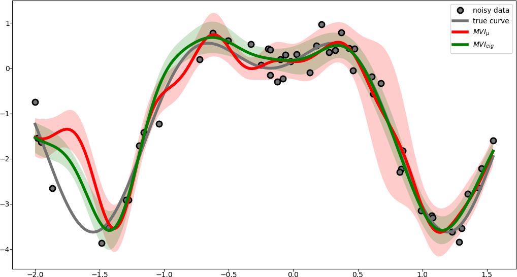
Figure 2: Regression task in Section V-B, on data corrupted with uniform noise. The mean predictions by MVI_$\mu$ (red) and MVI_eig (green) are plotted as solid lines. The shaded region around the means corresponds to $\pm$ 2 standard deviations of the predictions. Predictions are obtained through $S^{\prime}$ number of samples drawn from the corresponding approximating posterior $q(\mbox{\boldmath$w$})$.

We experiment with a regression task with $N=50$ input-target pairs $(x_{n},y_{n})$, $x_{n},\ y_{n}\in\mathbb{R}$. Inputs $x_{n}$ are drawn uniformly in $[-10.0,+10.0]$. Targets $y_{n}$ are generated through the expression

$$y_{n}=0.3x_{n}\sin(0.7x_{n})-0.03x_{n}^{2}$$ (15)

and corrupted with i.i.d. noise drawn from the uniform distribution with support $[-0.5,+0.5]$. This is a regression task where adopting a Gaussian likelihood would lead to poor results as it cannot adequately explain the noise. We adopt a Cauchy density instead. The unnormalised log-posterior reads:

$$\log\prod_{n=1}^{N}f(y_{n};\mbox{\boldmath$w$}^{T}\mbox{\boldmath$\phi$}_{n},\gamma)+\ln\mathcal{N}(\mbox{\boldmath$w$}|\mbox{\boldmath$0$},\alpha^{-1}\mbox{\boldmath$I$}_{D})\ ,$$ (16)

where $f(y;\mu,\gamma)=\left(\pi\gamma\ [1+(\frac{y-\mu}{\gamma})^{2}]\right)^{-1}$ is the Cauchy density. Additionally, we have calculated a set of $M$ radial basis functions on the data inputs:

$$\mbox{\boldmath$\phi$}_{n}=[\phi(\mbox{\boldmath$x$}_{n};r,\mbox{\boldmath$c$}_{1}),\ \dots,\ \phi(\mbox{\boldmath$x$}_{n};r,\mbox{\boldmath$c$}_{M}),\ 1]^{T}\ ,$$ (17)

where $\phi(\mbox{\boldmath$x$}_{n};r,\mbox{\boldmath$c$}_{m})=\exp(-\frac{\|\mbox{\boldmath$x$}_{n}-\mbox{\boldmath$c$}_{m}\|^{2}}{2r^{2}})$. The last element $1$ in (17) serves as a bias term. Hence, $\mbox{\boldmath$\phi$}_{n}\in\mathbb{R}^{M+1}$ and $\mbox{\boldmath$w$}\in\mathbb{R}^{D}$ with $D=M+1$.

In this numerical experiment, we generate $100$ datasets with $N=50$ training data items using (15). We also generate $N_{test}=1000$ test data items in precisely the same way. We report the median log-predictive density (LPD) on test data in Table II. Best performances are marked with bold. We see that the MVI_eig approximation performs the best, hence we mark it in bold. When looking at the results, we established that MVI_eig performs statistically significantly better than LA, MVI_$\mu$ and VI_diag. However, as MVI_eig  does not outperform MVI_lr  with statistical significance, we do not mark it additionally with $\bullet$ marker. In terms of error rate, we see that MVI_lr performs best and marginally better than MVI_eig. Finally, in figure 2 we show the true underlying curve, specified in (15), the observed training data as filled circles along with the regressions induced by MVI_$\mu$ and MVI_eig.

V-C Logistic Regression

TABLE III: Median LPD on test data for logistic regression over $100$ runs on the datasets (higher is better).

Dataset	Q	$N$	$N_{test}$	Laplace	MVI$\mu$	MVIeig	MVIlr	VIdiag
Banana	2	400	4900	-1238.76	-1219.19	-1221.41	$\mathbf{-1212.19}^{\bullet}$	-1253.36
Breast cancer	9	200	77	-42.82	-42.65	-42.53	$\mathbf{-42.38}$	-45.42
Diabetis	8	468	300	-145.98	-145.468	-145.31	$\mathbf{-144.89}^{\bullet}$	-193.27
Solar	9	666	400	-232.64	-232.37	-232.42	$\mathbf{-232.07}^{\bullet}$	-234.52
German	20	700	300	-151.71	-151.42	-151.31	$\mathbf{-150.70}^{\bullet}$	-179.29
Heart	13	170	100	-39.25	-38.973	-38.96	$\mathbf{-38.62}$	-48.37
Image	18	1300	1010	-304.33	-291.91	-284.19	-284.60	$\mathbf{-283.80}$
Ringnorm	20	400	7000	-309.87	$\mathbf{-308.80}$	-319.67	-309.80	-342.627
Splice	60	1000	2175	-1156.80	-900.00	$\mathbf{-897.33}$	-900.30	-899.501
Thyroid	5	140	75	-11.01	-10.189	-10.189	$\mathbf{-9.844}^{\bullet}$	-10.280
Titanic	3	150	2051	$\mathbf{-1018.92}^{\bullet}$	-1019.59	-1021.7	-1020.62	-1023.91
Twonorm	20	400	7000	-452.57	-450.716	-461.10	$\mathbf{-447.28}$	-543.115
Waveform	21	400	4600	-947.66	$\mathbf{-946.49}$	-948.62	-950.31	-969.61

TABLE IV: Median error rate $\%$ on test data for logistic regression over $100$ runs on the datasets (lower is better).

Dataset	Laplace	MVI$\mu$	MVIeig	MVIlr	VIdiag
Banana	11.76	11.49	11.53	$\mathbf{11.47}$	11.74
Breast cancer	28.95	28.84	28.84	$\mathbf{28.71}$	28.98
Diabetis	24.79	24.65	24.67	$\mathbf{24.38}$	34.33
Solar	35.15	35.14	35.16	$\mathbf{35.03}$	35.62
German	26.06	25.91	25.96	$\mathbf{25.75}$	29.00
Heart	18.05	17.81	17.68	$\mathbf{17.45}$	23.04
Image	13.96	13.38	12.86	13.14	$\mathbf{12.86}$
Ringnorm	1.95	$\mathbf{1.87}$	1.90	1.91	1.93
Splice	25.74	18.98	18.96	18.89	$\mathbf{18.71}$
Thyroid	6.35	6.08	6.09	$\mathbf{6.00}$	6.13
Titanic	$\mathbf{23.31}$	23.31	23.33	23.32	23.62
Twonorm	2.92	2.86	2.92	$\mathbf{2.84}$	2.96
Waveform	10.40	$\mathbf{10.33}$	10.36	10.34	10.44

We experiment with logistic regression [23, Chapter $4$]. The data are $N$ input-label pairs $(\mbox{\boldmath$x$}_{n},y_{n})$ with $\mbox{\boldmath$x$}_{n}\in\mathbb{R}^{Q},\ y_{n}\in\{0,1\}$. Just like in Section V-B, equation (17), we calculate a set of radial basis functions $\mbox{\boldmath$\phi$}_{n}\in\mathbb{R}^{M+1}$ on the data inputs $\mbox{\boldmath$x$}_{n}$. The weights are given by $\mbox{\boldmath$w$}\in\mathbb{R}^{D}$ with $D=M+1$. The unnormalised log-posterior reads:

$$\ln\prod_{n=1}^{N}\sigma(\mbox{\boldmath$\phi$}_{n}^{T}\mbox{\boldmath$w$})^{y_{n}}(1-\sigma(\mbox{\boldmath$\phi$}_{n}^{T}\mbox{\boldmath$w$}))^{1-y_{n}}+\ln\mathcal{N}(\mbox{\boldmath$w$}|\mbox{\boldmath$0$},\alpha^{-1}\mbox{\boldmath$I$}_{D})\ .$$ (18)

To avoid inadvertently selecting single datasets on which the proposed algorithm performs well, we experiment with the entire collection of datasets preprocessed by Rätsch et al. Each dataset has been standardised and split into $100$ training and testing instances, except for Image and Splice that have 20 splits. We approximate the log-posterior in (18) with LA, the MVI posteriors and VI_diag. To initialise the hyperparameters $\mbox{\boldmath$\theta$}=(M,r,\alpha,\mbox{\boldmath$c$}_{1},\dots,\mbox{\boldmath$c$}_{M})$ in Laplace, we proceed as follows: per dataset, we run LA for $10$ iterations for each combination of $M\in\{10,20,30\}$ and $10$ randomly drawn pairs $r\sim\mbox{Uniform}(0,1)$, $\alpha\sim\mbox{Uniform}(0,1)$, i.e. a total of $30$ combinations. The centres $\mbox{\boldmath$c$}_{m}$ are determined by K-means for each choice of $M$. The combination with the highest lower bound (we are maximising) is declared the winner and used to initialise LA which is then run for a maximum of $1000$ iterations. The MVI posteriors and hyperparameters in the respective objectives are initialised using the optimised Laplace posterior and hyperparameters, as described in Section III-D.

We report the median log-predictive density (LPD) on test data in Table III, along with details about the datasets. Best performances are marked with bold. Best performances that differ in a statistically significant way to all other performances (see Section IV-B) are additionally marked with a $\bullet$ marker. Table III reveals that, in general, the proposed MVI posteriors perform better than LA or VI_diag. In particular, we see that MVI_lr scores better on a number of datasets and that the difference in performance is often statistically significant. Table IV displays the results on error rates. We see that all methods achieved more or less the same error rates with no performance being statistically significantly superior. Nonetheless, we do observe a few exceptions, e.g. on datasets Splice and Diabetis LA and VI_diag respectively perform noticeably poorer.

V-D Multiclass Logistic Regression

TABLE V: Median LPD on test data for multiclass logistic regression over $100$ runs on the datasets (higher is better).

Dataset	K	Q	$N$	$N_{test}$	Laplace	MVI$\mu$	MVIeig	MVIlr	VIdiag
Ecoli	8	7	236	100	-50.32	-48.80	-49.31	$\mathbf{-48.52}^{\bullet}$	-51.39
Crabs	4	5	140	60	-64.59	-64.11	-64.28	$\mathbf{-64.10}$	-68.92
Iris	3	4	105	45	-9.06	-7.53	$\mathbf{-6.42}$	-7.46	-8.17
Soybean	4	35	33	14	-4.10	-2.35	$\mathbf{-0.66}^{\bullet}$	-2.36	-1.67
Wine	3	13	125	53	-5.72	-4.01	$\mathbf{-3.33}^{\bullet}$	-3.94	-4.66
Glass	6	9	150	64	-61.35	-60.39	$\mathbf{-59.79}$	-60.44	-76.26
Vehicle	4	18	593	293	-159.783	$\mathbf{-158.39}^{\bullet}$	-158.60	-159.15	-174.725
Balance	3	4	438	187	-23.5734	$\mathbf{-22.7321}$	-23.2197	-23.078	-31.587

TABLE VI: Median error rate $\%$ on test data for multiclass logistic regression over $100$ runs on the datasets (lower is better).

Dataset	Laplace	MVI$\mu$	MVIeig	MVIlr	VIdiag
Ecoli	17.22	16.75	17.23	$\mathbf{16.73}$	17.87
Crabs	55.75	$\mathbf{54.98}$	55.10	55.00	58.96
Iris	9.24	$\mathbf{7.57}$	7.86	7.58	9.76
Soybean	13.12	4.83	$\mathbf{3.85}^{\bullet}$	4.86	9.33
Wine	4.97	$\mathbf{3.11}$	3.31	3.14	4.72
Glass	42.93	41.14	$\mathbf{39.79}$	41.14	53.01
Vehicle	32.60	$\mathbf{32.15}$	32.34	32.22	34.61
Balance	6.56	$\mathbf{6.07}$	6.27	6.25	8.06

Similarly to logistic regression, multiclass logistic regression [23, Chapter $4$] does not allow direct Bayesian inference as the use of the softmax function renders integrals over the likelihood term intractable. The unnormalised log-posterior reads:

$$\ln\prod_{n=1}^{N}\prod_{k=1}^{K}p(C_{k}|\mbox{\boldmath$\phi$}_{n})^{y_{nk}}+\ln\prod_{k=1}^{K}\mathcal{N}(\mbox{\boldmath$w$}_{k}|\mbox{\boldmath$0$},\alpha^{-1}\mbox{\boldmath$I$}_{D})\ ,$$ (19)

where $K$ denotes the total number of classes. The data are input-label pairs $(\mbox{\boldmath$x$}_{n},\mbox{\boldmath$y$}_{n})$ with $\mbox{\boldmath$x$}_{n}\in\mathbb{R}^{Q}$. Vectors $\mbox{\boldmath$y$}_{n}$ are binary vectors encoding class labels using a $1$-of-$K$ coding scheme, e.g. $[0\ 1\ 0]$ encodes class label $2$ in a $3$-class problem. The probability $p(C_{k}|\mbox{\boldmath$\phi$}_{n})$ of the $n$-th data item belonging to class $C_{k}$ is modelled via the softmax function:

$$p(C_{k}|\mbox{\boldmath$\phi$}_{n})=\frac{\exp(\mbox{\boldmath$\phi$}_{n}^{T}\mbox{\boldmath$w$}_{k})}{\sum_{\ell=1}^{K}\exp(\mbox{\boldmath$\phi$}_{n}^{T}\mbox{\boldmath$w$}_{\ell})}\ ,$$ (20)

where each class $C_{k}$ is associated with a weight vector $\mbox{\boldmath$w$}_{k}\in\mathbb{R}^{D}$, with $D=M+1$. The basis functions $\mbox{\boldmath$\phi$}_{n}\in\mathbb{R}^{M+1}$ are defined in the same way as in Section V-B. We initialise hyperparameters $\mbox{\boldmath$\theta$}=(M,r,\alpha,\mbox{\boldmath$c$}_{1},\dots,\mbox{\boldmath$c$}_{M})$ in the same way as described in Section V-C.

To avoid inadvertently selecting single datasets on which the proposed algorithm performs well, we experiment with the collection of multiclass datasets used in the work of [27] in a different context. Details of the datasets are shown in Table V. We standardise the data column-wise to zero mean and unit standard deviation. Using random subsampling, we split each dataset $100$ times into a training ($70\%$ of the data) and testing ($30\%$) set. We report the median LPD for each dataset and algorithm in Table V and median error rate in Table VI. Again, best performances are marked in bold. We mark the best performance with a $\bullet$ marker if it is found to be statistically significant using the same two conditions described in Section IV-B. The results show an improvement over LA and the use of a factorised posterior in VI_diag. We also see that MVI_eig performs well on this set of problems in terms of LPD, though the picture is not as clear in terms of error rate in Table VI. Finally, we note the low performance of all methods on the dataset Crab, evidently in Table VI. This may be perhaps attributed to the particular choice of the RBF kernel made here, though other kernels (cf [27]) may be more appropriate.

VI Discussion and Conclusion

We proposed Mixed Variational Inference (MVI) as a method for approximate Bayesian inference in non-conjugate models. MVI makes use of the posterior obtained via the Laplace approximation and the objective function provided by variational inference. The adoption of the Laplace posterior helps with capturing a-posteriori correlations; the partial adaptation of the Laplace posterior, in the form of the proposed MVI posteriors, helps limit the number of free variational parameters that need to be optimised. The numerical results show that the MVI posteriors have the potential to improve on the performance of the Laplace approximation and on the performance of the commonly adopted factorised Gaussian posterior in variational inference.

Strictly speaking, however, one should be aware of the fact that a posterior $q(\mbox{\boldmath$w$})$ that approximates the true posterior better, does not necessarily guarantee improved log-predictive density; vice versa, a “naive” approximating posterior (e.g. factorised) may in principle provide satisfactory predictive performance. This observation has been previously stated in [3] where a variety of approximations are evaluated in the context of Gaussian process binary classification. Therein it is stated that, in principle, even a poor approximation in terms of posterior moments can still provide good predictions. After all, as far as variational approximations are concerned, it is evident in objective (3) that the goal is to find a $q(\mbox{\boldmath$w$})$ that is as close as possible to the true posterior; this does not necessarily correlate with improved predictive performance. Nevertheless, one does expect in practice that an approximation that captures posterior correlations in the parameters to be more useful than a factorised approximation that practically draws the parameters independently of one another when making predictions (see (13)). But beyond this expectation, it is admittedly difficult to anticipate what approximation may perform best. Indeed, in the numerical experiments we notice that while MVI_lr  seems well suited for logistic regression (see Table III), this is not necessarily the case in multiclass logistic regression (see Table V).

In its present form, MVI is limited to Gaussian posteriors. It would be interesting to extend MVI to non-Gaussian posteriors, though at first sight it seems that its dependence on the Laplace approximation considerably limits it. An interesting direction, inspired by [16], would be to postulate a posterior $q(\mbox{\boldmath$w$})$ based on a mixture of Gaussians, where the covariance of each Gaussian comes from a Laplace approximation performed at a different mode. Forming an approximating posterior using multiple modes procured by the Laplace approximation has been previously suggested in [28]. However, therein no objective function akin to (6) is guiding the inference of the posterior. This could be potentially addressed by extending MVI so that $q(\mbox{\boldmath$w$})$ is now a Gaussian mixture whose covariance matrices are given by the Laplace approximation and partially updated as suggested in Sections III-A, III-B, III-C. We reserve such investigations for future research.

References

- [1] D. J. MacKay, “A practical bayesian framework for backpropagation networks,” Neural computation, vol. 4, no. 3, pp. 448–472, 1992.
- [2] D. Sivia and J. Skilling, Data analysis: a Bayesian tutorial. OUP Oxford, 2006.
- [3] H. Nickisch and C. E. Rasmussen, “Approximations for binary gaussian process classification,” Journal of Machine Learning Research, vol. 9, no. Oct, pp. 2035–2078, 2008.
- [4] E. Eskin, A. J. Smola, and S. Vishwanathan, “Laplace propagation,” in Advances in neural information processing systems, 2004, pp. 441–448.
- [5] T. P. Minka, “Expectation propagation for approximate bayesian inference,” in Proceedings of the Seventeenth conference on Uncertainty in artificial intelligence. Morgan Kaufmann Publishers Inc., 2001, pp. 362–369.
- [6] B. S. Jensen, J. B. Nielsen, and J. Larsen, “Bounded gaussian process regression,” in Machine Learning for Signal Processing (MLSP), 2013 IEEE International Workshop on. IEEE, 2013, pp. 1–6.
- [7] A. Wu, N. G. Roy, S. Keeley, and J. W. Pillow, “Gaussian process based nonlinear latent structure discovery in multivariate spike train data,” in Advances in Neural Information Processing Systems, 2017, pp. 3496–3505.
- [8] M. J. Beal, “Variational Algorithms for Approximate Bayesian Inference,” Ph.D. dissertation, Gatsby Computational Neuroscience Unit, University College London, 2003.
- [9] D. Tzikas, C. Likas, and N. Galatsanos, “The Variational Approximation for Bayesian inference,” Signal Processing Magazine, IEEE, vol. 25, no. 6, pp. 131–146, 2008.
- [10] H. Soh, “Distance-preserving probabilistic embeddings with side information: Variational bayesian multidimensional scaling gaussian process.” in IJCAI, 2016, pp. 2011–2017.
- [11] A. Kabán, “On bayesian classification with laplace priors,” Pattern Recognition Letters, vol. 28, no. 10, pp. 1271–1282, 2007.
- [12] S. Yu, K. Yu, V. Tresp, and H.-P. Kriegel, “Variational bayesian dirichlet-multinomial allocation for exponential family mixtures,” in European Conference on Machine Learning. Springer, 2006, pp. 841–848.
- [13] J. Regier, A. Miller, J. McAuliffe, R. Adams, M. Hoffman, D. Lang, D. Schlegel, and M. Prabhat, “Celeste: Variational inference for a generative model of astronomical images,” in International Conference on Machine Learning, 2015, pp. 2095–2103.
- [14] M. A. Chappell, A. R. Groves, B. Whitcher, and M. W. Woolrich, “Variational bayesian inference for a nonlinear forward model,” IEEE Transactions on Signal Processing, vol. 57, no. 1, pp. 223–236, 2009.
- [15] M. W. Woolrich and T. E. Behrens, “Variational bayes inference of spatial mixture models for segmentation,” IEEE Transactions on Medical Imaging, vol. 25, no. 10, pp. 1380–1391, 2006.
- [16] S. J. Gershman, M. D. Hoffman, and D. M. Blei, “Nonparametric variational inference,” in Proceedings of the 29th International Coference on International Conference on Machine Learning. Omnipress, 2012, pp. 235–242.
- [17] J. Paisley, D. M. Blei, and M. I. Jordan, “Variational bayesian inference with stochastic search,” in Proceedings of the 29th International Coference on International Conference on Machine Learning. Omnipress, 2012, pp. 1363–1370.
- [18] T. Salimans, D. A. Knowles et al., “Fixed-form variational posterior approximation through stochastic linear regression,” Bayesian Analysis, vol. 8, no. 4, pp. 837–882, 2013.
- [19] M. Titsias and M. Lázaro-Gredilla, “Doubly stochastic variational bayes for non-conjugate inference,” in International Conference on Machine Learning, 2014, pp. 1971–1979.
- [20] D. P. Kingma and M. Welling, “Auto-encoding variational bayes,” arXiv preprint arXiv:1312.6114, 2013.
- [21] N. Gianniotis, C. Schnörr, C. Molkenthin, and S. S. Bora, “Approximate variational inference based on a finite sample of gaussian latent variables,” Pattern Analysis and Applications, vol. 19, no. 2, pp. 475–485, May 2016.
- [22] N. Depraetere and M. Vandebroek, “A comparison of variational approximations for fast inference in mixed logit models,” Computational Statistics, vol. 32, no. 1, pp. 93–125, 2017.
- [23] C. M. Bishop, Pattern Recognition and Machine Learning. Springer, 2006.
- [24] P. K. Mogensen and A. N. Riseth, “Optim: A mathematical optimization package for julia,” Journal of Open Source Software, vol. 3, no. 24, 2018.
- [25] P. Dalgaard, Introductory statistics with R. Springer Science & Business Media, 2008.
- [26] A. C. Davison, D. V. Hinkley et al., Bootstrap methods and their application. Cambridge university press, 1997, vol. 1.
- [27] I. Psorakis, T. Damoulas, and M. A. Girolami, “Multiclass Relevance Vector Machines: Sparsity and Accuracy,” IEEE Transactions on Neural Networks, vol. 21, no. 10, pp. 1588–1598, 2010.
- [28] A. Gelman, H. S. Stern, J. B. Carlin, D. B. Dunson, A. Vehtari, and D. B. Rubin, Bayesian data analysis. Chapman and Hall/CRC, 2013.