Averaged optical characteristics of an ensemble of metal nanoparticles

Abstract

A theory for the averaged optical characteristics of an ensemble of metal nanoparticles with different shapes has been developed. The theory is applicable both for the nanoparticle size at which the optical conductivity of the particle is a scalar and for the nanoparticle size at which the optical conductivity should be considered as a tensor. The averaged characteristics were obtained taking into account the influence of nanoparticle shape on the depolarization coefficient and the components of the optical conductivity tensor. The dependences of magnetic absorption by a spheroidal metal nanoparticle on the ratio between its curvature radii and the angle between the spheroid symmetry axis and the magnetic field vector were derived and theoretically considered. An original variant of the distribution function for nanoparticle shapes, which is based on the combined application of the Gaussian and “hat” functions, was proposed and analyzed.

I Introduction

A typical attribute of the optical spectra of ensembles of metal nanoparticle is the availability of plasma resonances. The number of those resonances, as well as their frequency positions and damping decrements, depend on the metal nanoparticle shape (see, e.g., Refs. 1 ; 2 ). Since it is hardly possible to create an ensemble of absolutely identical nanoparticles, experimenters, when studying the processes of light absorption and scattering by such ensembles, usually deal with averaged (apparent) optical characteristics. The procedure of averaging the optical characteristics for ensembles of spheroidal metal nanoparticles was described, e.g., in Refṡ. 3 ; 4 .

While examining the influence of the shape of metal nanoparticles on their optical properties, the authors of previous papers supposed that dissipative processes in nanoparticles are characterized by a scalar high-frequency conductivity. However, we have shown 2 ; 5 ; 6 that if the size of non-spherical nanoparticles does not exceed the electron free path length, the optical conductivity becomes a tensor quantity. The diagonal elements of this tensor together with the depolarization coefficients govern the half-widths of plasma resonances 2 ; 7 . In this case, the averaging over the nanoparticle shape is no more reduced to the averaging over the depolarization coefficients 3 . Therefore, in this paper, we consistently summarized the theoretical basis that was previously developed for the optical properties of an ensemble of elliptic metal nanoparticles, including the components of the optical conductivity tensor and the depolarization tensor 2 ; 5 ; 6 ; 7 . As a result, the depolarization coefficients and the components of the optical conductivity tensor averaged over the nanoparticle forms were calculated. While averaging over the nanoparticle shapes, the influence of this parameter on the conductivity was taken into account for the first time.

II Formulation of the problem

The study of optical properties of nanoparticles has a long history (see, e.g., Refs. 1 ; 3 ; 8 ; 9 ). In particular, the expression for the absorption cross-section of a plane electromagnetic wave with the frequency $\omega$ by a spherical nanoparticle which size is smaller than the wavelength has been known for a long time 10 :

$$K(\omega)=\frac{12\pi\,\omega\,a^{3}\epsilon^{\prime\prime}}{c}\left\{{\frac{1}{|\epsilon|^{2}}+\frac{\omega^{2}a^{2}}{90\,c^{2}}}\right\}.$$ (1)

Here, $c$ is the light velocity; $\epsilon$ the dielectric permittivity, which has the form

$$\epsilon=\epsilon^{\prime}+i\epsilon^{\prime\prime}=1-\frac{\omega_{p}^{2}}{\omega^{2}+\nu^{2}}+i\,\frac{\nu}{\omega}\frac{\omega_{p}^{2}}{\omega^{2}+\nu^{2}}$$ (2)

in the Drude model 1 ; $\nu$ is the bulk collision frequency;

$$\omega_{p}=\left(\frac{4\pi n_{0}e^{2}}{m}\right)^{1/2}$$ (3)

is the plasma frequency; and $e$, $m$, and $n_{0}$ are the electron charge, mass, and concentration, respectively. The first term in the braces in Eq. (1) is associated with the electric wave component, and the corresponding absorption is called electric absorption, whereas the second term is associated with the magnetic component and the corresponding absorption is called magnetic 10 .

The most general theory describing the optical properties of small particles, which simultaneously is the most cited one, is the Mie theory 11 . It was developed for spherical particles in the assumption that the vector of electric current density in the particle, $\mathbf{{j}}(\mathbf{{r}},t)$, is related to the generating field $\mathbf{{E}}(\mathbf{{r}},t)$ by Ohm’s law

$$\mathbf{{j}}(\mathbf{{r}},t)=\sigma\,\mathbf{{E}}(\mathbf{{r}},t),$$ (4)

where $\sigma$ is the scalar conductivity, $\mathbf{r}$ the coordinate vector, and $t$ the time. Generally speaking, relation (4) is valid for particles which sizes are much larger than the free electron path length 2 . Otherwise, this relation becomes non-local 12 , and, moreover, the conductivity becomes a tensor quantity in the case of asymmetric particles 2 .

Let a metal particle be in the field of an external electromagnetic wave

$$\left({\begin{array}[c]{l}\mathbf{{E}}\\ \mathbf{{H}}\end{array}}\right)=\left({\begin{array}[c]{l}\mathbf{{E}}^{(0)}\\ \mathbf{{H}}^{(0)}\end{array}}\right)\;e^{i\left({\mathbf{{k}}\mathbf{{r}}-\omega t}\right)},$$ (5)

where $\mathbf{E}$ and $\mathbf{H}$ are the electric and magnetic, respectively, components of the wave field; and $\mathbf{k}$ is the wave vector ($k=2\pi/\lambda$, where $\lambda$ is the wavelength). Then, the problem of finding the current density vector $\mathbf{{j}}(\mathbf{{r}},t)$, which governs the energy absorption, is split into two stages. At the first stage, we have to determine internal fields generated by wave (5) in the nanoparticle. At the second stage, we have to determine how these internal fields modify the electron velocity distribution function, i.e. to find a correction induced by the internal fields to the equilibrium Fermi distribution.

Since the internal fields induced by wave (5) in the nanoparticle depend on the particle shape, we will assume that the nanoparticle is an ellipsoid. It is convenient to develop a theory for this form, because the results obtained can be extended to a wide range of nanoparticle forms (from discoid- to rod-shaped) by changing the ellipsoid curvature radii.

If the wavelength $\lambda$ is much larger than the nanoparticle size ($\lambda\gg\max\left\{{R_{i}}\right\}$, where $R_{i}~{}(i=1,2,3)$ are the curvature radii), then the relation between the internal fields and external ones ($\mathbf{{E}}^{(0)}$ and $\mathbf{{H}}^{(0)}$) is known 10 . In particular, in the coordinate frame oriented along the principal ellipsoid axes, the electric (potential) component of the internal field has the form 10

$$(E_{in})_{j}=\frac{E_{j}^{(0)}}{1+L_{j}\left[\epsilon{(\omega)-1}\right]},$$ (6)

where $L_{j}$ is the $j$-th diagonal component of the depolarization tensor. Similarly, the eddy component of the electric field induced by the magnetic field $\mathbf{{H}}^{(0)}$ equals 2

$$(E_{ed})_{x}=i\frac{\,\omega\,}{c}\left\{{\frac{z\,H_{y}^{(0)}}{R_{z}^{2}+R_{y}^{2}}-\frac{y\,H_{x}^{(0)}}{R_{x}^{2}+R_{y}^{2}}}\right\}.$$ (7)

The other eddy field components can be obtained from Eq. (7) by cyclically permutating the subscripts. Let us also recall that $H^{(0)}=E^{(0)}$.

III Electron velocity distribution function and energy absorption by metal nanoparticles

The velocity distribution function of electrons in metal nanoparticles in the presence of fields (6) can be expressed as the sum of the equilibrium Fermi function $f_{0}(\varepsilon)$, where $\varepsilon=\frac{1}{2}mv^{2}$ is the electron energy, and the solution $f_{1}(\mathbf{{r}},\mathbf{{v}})$ of the kinetic equation linearized in the total (potential and eddy) field

$$\mathbf{{F}}=\mathbf{{E}}_{in}+\mathbf{{E}}_{ed};$$ (8)

namely,

$$(\nu-i\,\omega)\,f_{1}+\mathbf{{v}}\frac{\partial f_{1}}{\partial\mathbf{{r}}}+e\,\mathbf{{F}}(\mathbf{{r}})\mathbf{{v}}\frac{\partial f_{0}}{\partial\varepsilon}=0.$$ (9)

The function $f_{1}(\mathbf{{r}},\mathbf{{v}})$ must also satisfy the boundary condition

$$\left.{f_{1}(\mathbf{{r}},\mathbf{{v}})}\right|_{S}=0~{}\mathrm{at~{}}v_{n}<0,$$ (10)

where $v_{n}$ is the velocity component directed normally to the surface. The solution of the boundary problem (9), (10) for the ellipsoidal particle looks like

$$f_{1}(\mathbf{{r}},\mathbf{{v}})=-{f}_{0}^{\prime}(\varepsilon)\int\limits_{0}^{t_{0}}{d\tau\,e^{-\tilde{{\nu}}(t_{0}-\tau)}e\,\mathbf{{F}}({\mathbf{{r}}}^{\prime}-{\mathbf{{v}}}^{\prime}(t_{0}-\tau))}.$$ (11)

Here, $\tilde{{\nu}}=\nu-i\,\omega$, and

$$t_{0}=\frac{1}{{v}^{\prime}{}^{2}}\left[{\mathbf{{r}}}^{\prime}{\mathbf{{v}}}^{\prime}+\sqrt{(R^{2}-{r}^{\prime}{}^{2}){v}^{\prime}{}^{2}+({\mathbf{{r}}}^{\prime}{\mathbf{{v}}}^{\prime})^{2}}\right]$$ (12)

is a characteristic of Eq. (9). The primes in Eqs. (11) and (12) mark the corresponding quantities in a deformed coordinate frame, in which the ellipsoidal particle becomes spherical 2 . The coordinate and velocity components in the deformed and undeformed frames are mutually related:

$$x_{j}=\frac{R_{j}}{R}{x}_{j}^{\prime},\quad v_{j}=\frac{R_{j}}{R}{v}_{j}^{\prime},\quad(j=1,2,3),$$ (13)

where $R=(R_{1}R_{2}R_{3})^{1/3}$.

Knowing the electron velocity distribution function, the current density vector can be found:

$$\mathbf{{j}}(\mathbf{{r}},\omega)=\mathrm{Re}\left({\frac{m}{2\pi\hbar}}\right)^{3}\int{\mathbf{{v}}\,f_{1}(\mathbf{{r}},\mathbf{{v}})}\,d^{3}(v).$$ (14)

In accordance with Eqs. (8) and (11), this vector has two components: the electric and magnetic ones induced by $\mathbf{{E}}_{in}$ and $\mathbf{{E}}_{ed}$, respectively:

$$\mathbf{{j}}(\mathbf{{r}},\omega)=\mathbf{{j}}_{e}(\mathbf{{r}},\omega)+\mathbf{{j}}_{m}(\mathbf{{r}},\omega),$$ (15)

The explicit forms can be determined for both components by substituting Eq. (11) into Eq. (14).

Accordingly, the energy absorbed by the metal nanoparticle,

$$W=W_{e}+W_{m}=\frac{1}{2}\mathrm{Re}\int\limits_{V}{d\,\mathbf{{r}}}\left\{{\mathbf{{j}}_{e}\,\mathbf{{E}}_{in}^{\ast}+\mathbf{{j}}_{m}\,\mathbf{{E}}_{ed}^{\ast}}\right\},$$ (16)

is also the sum of the electric and magnetic contributions. By normalizing Eq. (16) to the magnitude of the flux incident on the nanoparticle, we obtain the absorption coefficients. For example, the coefficient of electric light absorption by a metal particle of the volume $V$ located in a matrix with the dielectric constant $\epsilon_{m}$ equals

$$K\left(\omega\right)=4\pi\,\mathrm{Re}\int\limits_{V}{d\mathbf{{r}}}\frac{{\mathbf{{j}}_{e}\left({\mathbf{{r}},\omega}\right)\mathbf{{E}}_{in}^{\ast}\left({\mathbf{{r}},\omega}\right)}}{{c\sqrt{\epsilon_{m}}|E^{\left(0\right)}|^{2}}}.$$ (17)

IV Optical parameters of an ensemble of spheroidal metal nanoparticles

Below, an ensemble of spheroidal (ellipsoid of rotation) metal nanoparticles is considered. This shape is the simplest among asymmetric ones, because its asymmetry is characterized by a single dimensionless parameter: either the ratio between the spheroid curvature radii , $\rho=R_{\bot}/R_{||}$, or the spheroid eccentricity $e_{p}=\sqrt{\left|{1-\rho^{2}}\right|}$. In this case, the obtained theoretical results can be applied to explain the optical properties of particles within a wide interval of shapes, from discoid to rod-like, by simply changing the curvature radii.

First of all, we are interested in how the dispersion of nanoparticle shapes affects the optical characteristics of nanoparticle ensemble. Recall that the nanoparticle form governs the frequencies and the number of plasma resonances. Therefore, in order to emphasize the shape effect, let us assume that the nanoparticles in the ensemble have the same volume $V$, but different eccentricities $e_{p}$’s.

The coefficient of electric light absorption by a single spheroidal metal nanoparticle can be obtained as the sum

$$K\left({\omega,\rho}\right)=\,K_{\bot}\left({\omega,\rho}\right)+K_{||}\left({\omega,\rho}\right),$$ (18)

where each $s$-th component $(s=\bot,\|)$ is determined by Eq. (17), so that

$$K_{s=\bot,\|}\left({\omega,\rho}\right)\\ =\dfrac{\mu_{s}\,\omega^{4}\sigma_{s}\left({\omega,\rho}\right)}{\left[(\omega^{2}-\omega_{s}^{2})g_{s}(\rho)\right]^{2}+\left[4\pi\,L_{s}(\rho)\sigma_{s}(\omega,\rho)\omega\right]^{2}}.$$ (19)

Here, the averaging over the orientations of the spheroid symmetry axis has already been made, and the following notations are introduced:

$$\begin{array}[c]{l}\mu_{||}=\dfrac{4\pi\epsilon_{m}^{3/2}}{3c},\quad\mu_{\bot}=2\mu_{||},\\ g_{s}(\rho)=\epsilon_{m}+L_{s}(\rho)\,(1-\epsilon_{m});\end{array}$$ (20)

the quantities

$$\omega_{s}(\rho)=\omega_{p}\sqrt{\frac{L_{s}(\rho)}{g_{s}(\rho)}}$$

are the frequencies corresponding to collective (plasma) oscillations of conduction electrons in the nanoparticles in the directions perpendicularly $(s=\perp)$ and in parallel $(s=\|)$ to the spheroid symmetry axis; and $\sigma_{\bot,\parallel}(\omega,\rho)$ are the components of the optical conductivity tensor.

In the coordinate frame with the axis $OZ$ directed along the spheroid symmetry axis, the diagonal components of the optical conductivity tensor look like

$$\sigma_{xx}=\sigma_{yy}\equiv\sigma_{\bot},\quad\sigma_{zz}\equiv\sigma_{\parallel}.$$ (21)

Analogously,

$$L_{x}=L_{y}\equiv L_{\bot},\quad L_{z}=L_{\parallel}.$$ (22)

The principal values of the depolarization tensor are

$$L_{\bot} =\frac{1}{2}(1-L_{||}),$$ (23)

$$L_{||} =\left\{{\begin{array}[c]{ll}\dfrac{1-e_{p}^{2}}{2e_{p}^{3}}\left[\ln\left({\dfrac{1+e_{p}}{1-e_{p}}}\right)-2e_{p}\right]&\mathrm{for}~{}\rho<1,\\ \dfrac{1+e_{p}^{2}}{e_{p}^{3}}(e_{p}-\arctan e_{p})&\mathrm{for}~{}\rho>1.\end{array}}\right.$$ (26)

In Refs 2 ; 5 , it was shown that, if a non-spherical metal nanoparticle is smaller than the electron free path length in it, the optical conductivity becomes a tensor quantity, unlike the spherical case, where it is a scalar. The components of this tensor were also analyzed in Refs 2 ; 5 in the general case of ellipsoidal nanoparticles and in various limiting cases. Here, we are interested in the non-zero components of the optical conductivity tensor for spheroidal nanoparticles, $\sigma_{\bot}$ and $\sigma_{||}$. Let us confine the consideration to the case when the influence of the nanoparticle shape on the optical conductivity tensor components is maximum. Expression (11) makes allowance for both the bulk (by means of the parameter $\nu$) and the surface (by means of the characteristic $t_{0}$) electron scattering. The mere surface electron scattering can be formally obtained from Eq. (11) by putting $\nu\rightarrow 0$. Actually, we mean the inequality $\nu\ll v_{F}/R$, i.e. the bulk collision frequency is small in comparison with the frequency of electron oscillations between the nanoparticle walls. As a result, we obtain (for more details, see Refs 2 ; 5 ) that

$$\sigma_{\bot}=\frac{3\sigma_{0}}{16}\times\left\{{\begin{array}[c]{ll}\dfrac{\left({1-e_{p}^{2}}\right)^{1/3}}{e_{p}^{3}}\left[{e_{p}\left({1+2e_{p}^{2}}\right)-}\dfrac{{\left({1-4e_{p}^{2}}\right)}}{{\left({1-e_{p}^{2}}\right)^{1/2}}}{\arcsin e_{p}}\right]&\mathrm{for}~{}\rho<1,\\ \dfrac{\left({1+e_{p}^{2}}\right)^{1/3}}{e_{p}^{3}}\left[{-e_{p}\left({1-2e_{p}^{2}}\right)+}\dfrac{{\left({1+4e_{p}^{2}}\right)}}{{\left({1+e_{p}^{2}}\right)^{1/2}}}{\ln\left({e_{p}+\sqrt{1+e_{p}^{2}}}\right)}\right]&\mathrm{for}~{}\rho>1,\end{array}}\right.$$ (27)

$$\sigma_{||}=\frac{3\sigma_{0}}{8}\times\left\{{\begin{array}[c]{ll}\dfrac{\left({1-e_{p}^{2}}\right)^{1/3}}{e_{p}^{3}}\left[{-e_{p}\left({1-2e_{p}^{2}}\right)+}\dfrac{1}{{\left({1-e_{p}^{2}}\right)^{1/2}}}{\arcsin e_{p}}\right]&\mathrm{for}~{}\rho<1,\\ \dfrac{(1+e_{p}^{2})^{{}^{1/3}}}{e_{p}^{3}}\left[{e_{p}\left({1+2e_{p}^{2}}\right)-}\dfrac{1}{{\left({1+e_{p}^{2}}\right)^{1/2}}}{\ln\left({e_{p}+\sqrt{1+e_{p}^{2}}}\right)}\right]&\mathrm{for}~{}\rho>1.\end{array}}\right.$$ (28)

Here,

$$\sigma_{0}=\frac{3n_{0}e^{2}}{2m\omega^{2}}\nu_{s}=\frac{n_{0}e^{2}}{m\omega^{2}}\left({\frac{3}{4}\frac{v_{F}}{R}}\right)$$ (29)

is the well-known expression for the optical conductivity of spherical nanoparticle, in which

$$\nu_{s}=\frac{{v_{F}}}{2R}$$ (30)

is the electron oscillation frequency between the walls, $v_{F}$ is the Fermi velocity, and $R$ the radius of spherical particle. For an ellipsoidal nanoparticle, the parameter $\nu_{s}$ is the electron oscillation frequency between the walls but in a spherical nanoparticle with the same volume. One can see that the both results (27) and (28) tends to formula (29), if the nanoparticle shape approaches the spherical one (at $e_{p}\rightarrow 0$). In expressions (27) and (28), we omitted the oscillatory terms associated with the frequency resonance between the external electromagnetic wave and the electron oscillations between the walls. In the visible spectral interval, this resonance is not significant (for more details, see Refs. 13 ; 14 ).

Therefore, the principal values of not only the depolarization tensor [see Eqs. (23) and (26)], but also of the optical conductivity tensor [Eqs. (27) and (28)], depend on the nanoparticle shape described by the eccentricity $e_{p}$ (or the curvature radius ratio $\rho$). Therefore, the both dependencies have to be taken into account when averaging over the shape spread.

In Fig. 1(a), the dependence $K\left({\lambda,\rho}\right)$ of the coefficient $K$ of electric light absorption by a spheroidal nanoparticle averaged over the nanoparticle orientation on the electromagnetic wave length $\lambda$ and the nanoparticle shape described by the curvature radius ratio $\rho$ is depicted. Two ridges correspond to two plasma resonances, which mutually intersect at the $\left({\lambda,\rho}\right)$-point with $\rho=1$ corresponding to the plasma resonance in a spherical nanoparticle. Panel (a) only exhibits a local fragment of the dependence $K\left({\lambda,\rho}\right)$. For a more complete understanding of the behavior of indicated plasma resonances, panel (b) illustrates their traces $K_{\bot}^{t}$ and $K_{||}^{t}$ in a wider area of the plane $\left({\lambda,\rho}\right)$.

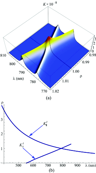
Figure 1: (Color online) (a) Dependence of the coefficient $K$ of electric light absorption by a spheroidal nanoparticle averaged over the nanoparticle orientation on the electromagnetic wave length $\lambda$ and the nanoparticle shape described by the curvature radius ratio $\rho$. (b) Traces of plasma resonances $K_{\bot}^{t}$ and $K_{||}^{t}$ in the plane $\left({\lambda,\rho}\right)$.

In order to obtian an expression for the total light absorption coefficient for an ensemble of metal nanoparticles that takes into account the spread of particle shapes, expression (18) has to be averaged with the weigh $\Pi(\rho)$. The latter describes the probability to find a nanoparticle with the given $\rho$-value in the ensemble. We assume the function $\Pi(\rho)$ to be normalized to the nanoparticle concentration $N$:

$$\int\limits_{0}^{\infty}{\Pi\left(\rho\right)}\,d\rho=N,$$ (31)

In terms of the function $P(\rho)=\frac{1}{N}{\Pi\left(\rho\right)}$, the apparent value of the total absorption coefficient reads

$$\overline{K\left(\omega\right)}=\int\limits_{0}^{\infty}{K\left({\omega,\rho}\right)P\left(\rho\right)}\,d\rho.$$ (32)

V Selection of the function $P(\rho)$

The function $P(\rho)$ is nothing else but a probability to find a nanoparticle with a definite $\rho$-value from the interval $0\leq\rho<\infty$. It can be considered as the probability density for the function $K\left({\omega,\rho}\right)$, so that Eq. (32) describes the averaging of the total absorption coefficient of the nanoparticle ensemble over the nanoparticle shapes.

While constructing $P(\rho)$, let us firstly pay attention that its domain includes only non-negative $\rho$-values, so that

$$P(\rho<0)=0.$$ (33a)

Let the distribution $$P(\rho) \rho \rho=a 0<\rho<a \rho>a R_{\bot}\geq aR_{||}$$ be characterized by a maximum at a certain -value , which separates the regions of “oblate” () and “prolate” () particles. Let the shape distribution of “prolate” particles () be described by the Gaussian function

$$P(\rho>a)=\alpha\exp[-\beta_{1}(\rho-a)^{2}]\,,$$ (33b)

where the parameters $$\alpha \beta_{1}$$ and have a clear meaning.

The expression for the function $P(\rho)$ within the “oblate” interval $0\leq\rho\leq a$ was chosen to satisfy the continuity conditions at its ends, i.e. $P(\rho=0)=0$ and $P(\rho=a+0)=P(\rho=a-0)=\alpha$. For this purpose, we selected the function

$$P(0\leq\rho\leq a)=\alpha\exp\left[{-\frac{\beta_{0}\,(\rho-a)^{2}}{a^{2}-(\rho-a)^{2}}}\right],$$ (33c)

which is an extention of Sobolev’s “hat” function 15 ; 16 . The meaning of the parameters $\alpha$ and $\beta_{0}$ in Eq. (33c) is also quite clear. The properties of Sobolev’s “hat” function make it very attractive for the solution of a good many problems 17 . An additional advantage of this choice is a high smoothness of the resulting “cap” function (33) within the whole interval of its definition, because both Gaussian (33b) and function (33c) are infinitely differentiable ones. The value of the parameter $\alpha$ corresponds to the maximum value of the function $P(\rho)$ at $\rho=a$ and is determined from the normalization condition $\int\limits_{0}^{\infty}{P(\rho)\,d\rho}=1$.

The proposed model function $P(\rho)$ was selected on the heuristic principle. Its application strongly simplifies the solution of a rather complicated problem concerning the influence of the metal nanoparticle shape dispersion on the total absorption coefficient of nanoparticle ensemble. The functions describing the size distribution of nanoparticles 18 ; 19 are an argument in favor of our choice.

The illustrative calculations below were made for three parameter sets (I, II, and III) of the function ${P(\rho)}$, which are quoted in Table 1. The corresponding plots are depicted in Fig. 2.

Table 1: Parameter sets of the function $P(\rho)$.

Variant	$a$	$\beta_{0}$	$\beta_{1}$	$\alpha$
I	1.0	1.0	1.638	0.772
II	1.0	0.194	0.262	0.391
III	2.0	1.0	0.410	0.386

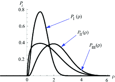
Figure 2: (Color online) ‘‘Cap’’ probability functions $P_{\mathrm{I,II,III}}(\rho)$ describing the distributions of nanoparticles over their shape.

VI Results of computational experiment and their interpretation

In computations, the following values of problem parameterswere used: $\omega_{p}=1.37\times 10^{16}~{}\mathrm{s}^{-1}$, $\nu=3.39\times 10^{13}~{}\mathrm{s}^{-1}$, $R=2.0\times 10^{-6}~{}\mathrm{cm}$, $c=3.0\times 10^{10}~{}\mathrm{cm/s}$, $v_{F}=1.39\times 10^{8}~{}\mathrm{cm/s}$, $n=10^{22}~{}\mathrm{cm}^{-3}$, $m=9.11\times 10^{-27}~{}\mathrm{g}$, and $\epsilon_{m}=16.$

One of the results obtained for the dependence $K\left({\lambda,\rho}\right)$ of the absorption coefficient for a spheroidal metal nanoparticle is shown in Fig. 1(a). This figure illustrates the dependence $K\left({\lambda,\rho}\right)$ in the vicinity of resonance with the external electromagnetic field for nanoparticles which forms are close to the spherical one ($\rho=1$). Let us also introduce two functions, $K_{\bot}^{(\max)}(\rho)$ and $K_{||}^{(\max)}(\rho)$, corresponding to the first and second components, respectively, in Eq. (18). They are projections of the maximum values of the orthogonal ($\perp$) and parallel ($\parallel$) components of the light absorption coefficient $K\left({\omega,\rho}\right)$ for the spheroidal metal nanoparticle onto the plane $(K,\rho)$ [see Fig. 3(a)]. (In what follows, it is more convenient to use the frequency dependence of sought coefficients, taking into account the dependences of the plasma resonance frequencies on the nanoparticle shape.) In other words, $K_{\bot}^{(\max)}(\rho)$ and $K_{||}^{(\max)}(\rho)$ are projections of two ridges in the dependence $K\left({\omega,\rho}\right)$ corresponding to two plasma resonances (Fig. 1) onto the plane $(K,\rho)$ [Fig. 3(a)]. Three segments in Fig. 3(a) illustrates the half-widths of the functions $P_{i}(\rho)$ ($i=\mathrm{I},\mathrm{II},\mathrm{III}$). The $x$-coordinates $\rho_{a}$ and $\rho_{b}$ of segment ends coincide with the calculated values $\rho_{a}^{(\mathrm{I})}\approx 0.36$, $\rho_{b}^{(\mathrm{I})}\approx 1.65$, $\rho_{a}^{(\mathrm{II})}\approx 0.13$, $\rho_{b}^{(\mathrm{II})}\approx 2.63$, $\rho_{a}^{(\mathrm{III})}\approx 0.72$, and $\rho_{b}^{(\mathrm{III})}\approx 3.30$. The ordinate positions of those segments are irrelevant.

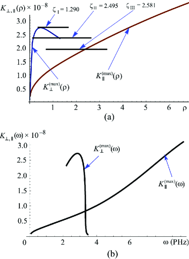
Figure 3: (Color online) (a) Projections $K_{\bot}^{(\max)}(\rho)$ and $K_{||}^{(\max)}(\rho)$ of the maximum values of the orthogonal and parallel components of the absorption coefficient $K\left({\omega,\rho}\right)$ for the spheroidal metal nanoparticle onto the plane $(K,\rho)$, and the segments corresponding to the half-widths of the functions $P_{i}(\rho)$ $(i=\mathrm{I\,,II\,,III})$. (b) The same as in panel (a), but the projections $K_{\bot}^{(\max)}(\omega)$ and $K_{||}^{(\max)}(\omega)$ are made onto the plane $(K,\omega)$.

Similarly, the functions $K_{\bot}^{(\max)}(\omega)$ and $K_{||}^{(\max)}(\omega)$ are the projections of the maximums of the orthogonal and parallel, respectively, components of the absorption coefficient by a spheroidal metal nanoparticle onto the plane $(K,\omega)$ [Fig. 3(b)].

First of all, attention is attracted by the fact that the domain of the orthogonal component (ridge) of the light absorption coefficient, $K_{\bot}\left({\omega,\rho}\right)$, is very narrow. Really, as follows from calculations, the function $K_{\bot}^{(\max)}(\rho)$ is determined in the interval $\rho\in(0,1.414)$ [Fig. 3(a)], whereas the domain of the function $K_{\bot}^{(\max)}(\omega)$ is the interval $\omega\in(2.14\times 10^{15}~{}\mathrm{s}^{-1},3.47\times 10^{15}~{}\mathrm{s}^{-1})$ [Fig. 3(b)]. On the other hand, from the dependence of the plasma resonance frequency on the nanoparticle shape, it follows that the transverse resonance frequency $\omega_{\bot}(\rho)$ falls within the interval $(2.14\times 10^{15}~{}\mathrm{s}^{-1},3.32\times 10^{15}~{}\mathrm{s}^{-1})$. (We conventionally call plasma oscillations in the directions along the spheroid axis and perpendicularly to it as longitudinal and transverse, respectively.) Thus, the domain of the function $K_{\bot}^{(\max)}(\omega)$ is composed of two sections: the resonance, $\omega_{r}\in(2.14\times 10^{15}~{}\mathrm{s}^{-1},3.32\times 10^{15}~{}\mathrm{s}^{-1})$, and the deflation, $\omega_{d}\in[3.32\times 10^{15}~{}\mathrm{s}^{-1},3.47\times 10^{15}~{}\mathrm{s}^{-1})$, ones. In the latter, $K_{\bot}^{(\max)}(\omega)$ drastically decreases to the background values of $K\left({\omega,\rho}\right)$ (In geology, deflation is the process of the particle dispersing and removal by the wind.) It is also important to mark that there is a single plasma resonance in $K_{||}\left({\omega,\rho}\right)$ at $\omega>3.47\times 10^{15}~{}\mathrm{s}^{-1}$.

The main aim of the computational experiment was to determine the apparent values of the total absorption coefficient,

$$\overline{K_{i}\left(\omega\right)}=\int\limits_{0}^{\infty}{K\left({\omega,\rho}\right)P_{i}\left(\rho\right)}\,d\rho\;,$$ (34)

for various functions $P_{i}(\rho)$ $(i=\mathrm{I,\,II,\,III})$. The corresponding results are shown in Fig. 4.

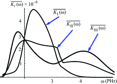
Figure 4: (Color online) Averaged dependencesof the total absorption coefficient $\overline{K\left(\omega\right)}$ for ensembles of spheroidal nanoparticle with various nanoparticle-shape distribution functions ${P_{i}\left(\rho\right)}$ ($i=\mathrm{I,II,III}$).

By comparing the spectral dependence of the total light absorption coefficient for a single spheroidal metal nanoparticle (Fig. 1) with the same dependence for nanoparticle ensembles (Fig. 4), we arrive at a conclusion that the corresponding values differ from one another by about two orders of magnitude. This ratio is rather general. Let us consider the plots of the functions $\overline{K_{i}\left(\omega\right)}$ (Fig. 4) in more detail.

A comparison between the plots of the functions $K_{\bot}^{(\max)}(\rho)$ and $K_{||}^{(\max)}(\rho)$, on the one hand, and the half-widths $\zeta_{i}$ of the functions $P_{i}(\rho)$ $(i=\mathrm{I\,,II\,,III})$, on the other hand, brings us to the following conclusions.

$\bullet$ The main factor “affecting” the function $P_{I}(\rho)$ at integral transformation (34) is the orthogonal component $K_{\perp}\left({\omega,\rho}\right)$ of the coefficient of light absorption by a spheroidal metal nanoparticle $K\left({\omega,\rho}\right)$ [cf. $K_{\bot}^{(\max)}(\rho)$ and $\zeta_{I}$ in Fig. 3(a)]. Therefore, in the resonance region $\omega_{r}$, the curve $\overline{K_{I}\left(\omega\right)}$ in Fig. 4 is, in a sense, similar to its “parent” $P_{I}(\rho<1.414)$. The behavior of the curve $\overline{K_{I}\left(\omega\right)}$ in Fig. 4 appreciably changes in the deflation section $\omega_{d}$.

$\bullet$ The function $\overline{K_{II}\left(\omega\right)}$ changes the most substantially in the deflation section $\omega_{d}$ and its right wing, where the influence of $K_{||}^{(\max)}(\rho>1.414)$ and $K_{||}^{\max}(\omega>3.47\times 10^{15}~{}\mathrm{s}^{-1})$ is appreciable.

$\bullet$ The function $\overline{K_{III}\left(\omega\right)}$ most adequately describes the real situation. It completely takes into account the influence of both the transversal $K_{\bot}\left({\omega,\rho}\right)$ and longitudinal $K_{||}\left({\omega,\rho}\right)$ components of the light absorption coefficient on $P_{III}(\rho)$.

VII Magnetic absorption

Let us consider the frequency interval

$$\nu\ll\omega\ll\omega_{s}\quad(s=\bot,||).$$ (35)

For typical metals, $\nu\sim 10^{13}~{}\mathrm{s}^{-1}$. The inequality $\nu\ll\omega$ allows us to neglect the bulk scattering of electrons. The inequality $\omega\ll\left(\omega_{\bot},\omega_{||}\right)$ means that we are far from plasma resonances, and the electrical absorption does not “obscure” the magnetic one . By substituting Eq. (14) into Eq. (16), we obtain the following expression for the energy of magnetic light absorption by a spheroidal ($R_{1}=R_{2}\equiv R_{\bot}$, $R_{3}\equiv R_{||}$) metal nanoparticle 5 ; 22 :

$$W_{m}=\frac{9}{128}V\frac{n\,\,e^{2}}{mc^{2}}v_{F}R_{\bot}\\ \times\left[{\chi_{H}\left({H_{||}^{(0)}}\right)^{2}+\eta_{H}\left({\frac{R_{||}^{2}}{R_{\bot}^{2}+R_{||}^{2}}H_{\bot}^{(0)}}\right)^{2}}\right].$$ (36)

Here, $H_{||}^{(0)}$ and $H_{\bot|}^{(0)}$ are the amplitudes of the magnetic wave field components that are parallel ($\parallel$) and orthogonal ($\perp$) to the rotation axis of spheroid. Formula (36) includes only the magnetic components, because they are engaged in the magnetic light absorption by a nonspherical nanoparticle. Finally,

$$\chi_{H}=\dfrac{1}{8e_{p}^{2}}\times\left\{{\begin{array}[c]{ll}\left({1+2e_{p}^{2}}\right)\left({1-e_{p}^{2}}\right)^{1/2}-\dfrac{{1-4e_{p}^{2}}}{e_{p}}\arcsin e_{p}&\mathrm{for~{}}\rho<1,\\ -\left({1-2e_{p}^{2}}\right)\left({1+e_{p}^{2}}\right)^{1/2}+\dfrac{{1+4e_{p}^{2}}}{e_{p}}\ln\left({e_{p}+\sqrt{1+e_{p}^{2}}}\right)&\mathrm{for~{}}\rho>1;\end{array}}\right.$$ (37)

$$\eta_{H}=\frac{1}{4e_{p}^{2}}\times\left\{{\begin{array}[c]{ll}-\left({1-8e_{p}^{2}+4e_{p}^{4}}\right)\left({1-e_{p}^{2}}\right)^{1/2}+\dfrac{{1+2e_{p}^{2}}}{e_{p}}\arcsin e_{p}&\mathrm{for~{}}\rho<1,\\ \left({1+8e_{p}^{2}+4e_{p}^{4}}\right)\left({1+e_{p}^{2}}\right)^{1/2}-\dfrac{{1-2e_{p}^{2}}}{e_{p}}\ln\left({e_{p}+\sqrt{1+e_{p}^{2}}}\right)&\mathrm{for~{}}\rho>1.\end{array}}\right.$$ (38)

In the case of spherical nanoparticle, $R_{\bot}=R_{||}=a$, i.e. $e_{p}\rightarrow 0$, so that $\chi_{H}=2/3$ and $\eta_{H}=8/3$, and we obtain the result of Ref. 5 ,

$$W_{m}^{(0)}=\frac{3}{64}V\frac{n\,\,e^{2}v_{F}}{mc^{2}}a\left({H^{(0)}}\right)^{2}.$$ (39)

In what follows, when studying the dependence of absorption by a nanoparticle on its shape, it is convenient to consider the ratio between the energy absorbed by a spheroidal particle and the energy absorbed by a spherical particle with the same volume, i.e. the ratio of expressions (36) and (39):

$$\frac{W_{m}}{W_{m}^{(0)}}=\frac{3}{2}\rho^{1/3}\frac{\chi_{H}\left({H_{||}^{(0)}}\right)^{2}+\dfrac{\eta_{H}}{(1+\rho^{2})^{2}}\left({H_{\bot}^{(0)}}\right)^{2}}{\left({H^{(0)}}\right)^{2}}.$$ (40)

When deriving this formula, we took into account that

$$\frac{R_{\bot}}{a}=\frac{R_{\bot}}{(R_{\bot}^{2}R_{||})^{1/3}}=\rho^{1/3}.$$

Ratio (40) is also equal to the ratio between the absorption coefficients of spheroidal and spherical nanoparticles. In the coordinate frame oriented along the principal spheroid axes,

$$H_{||}^{(0)}=H^{(0)}\cos\theta,\quad H_{\bot}^{(0)}=H^{(0)}\sin\theta,$$ (41)

where $\theta$ is the angle between the vector $\mathbf{H}^{(0)}$ and the spheroid axis of rotation. As a result, we obtain

$$\frac{W_{m}}{W_{m}^{(0)}}=\frac{3}{2}\rho^{1/3}\left[\chi_{H}\cos^{2}\theta+\frac{\eta_{H}}{(1+\rho^{2})^{2}}\sin^{2}\theta\right].$$ (42)

A 3D plot demonstrating the dependence of this ratio on the variables $\rho$ and $\theta$ is shown in Fig. 5. The adequacy of the plotted geometric surface to the physical picture is evidenced by the following facts. First of all, attention is drawn by a boundary between two surface sections, convex (at $0\leq\rho<1$) and concave (at $\rho>1$) ones. This boundary is a straight line, with its every point satisfying the equality

$$W_{m}(\rho=1,0\leq\theta\leq\pi)=W_{m}^{(0)}.$$

From the physical viewpoint, this equality is confirmed by a simple fact: for a particle with $\rho=R_{\bot}/R_{||}=1$, the absorbed energy is identical to that adsorbed by a spherical particle, $W_{m}(\rho=1,\theta)=W_{m}^{(0)}$, irrespective of the angle $\theta$ between the vector $\mathbf{H}^{(0)}$ and the axis of sphere rotation.

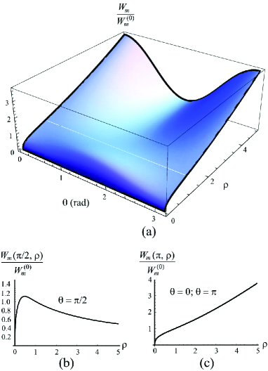
Figure 5: (Color online) (a) 3D plot demonstrating the dependence of the magnetic energy $W_{m}(\rho,\theta)$ absorbed by a spheroidal particle on its shape (the parameter $=R_{\bot}/R_{||}$) and orientation with respect to the electromagnetic wave vector (the angle $\theta$). The values are normalized by the energy $W_{m}^{(0)}$ absorbed by a spherical particle. (b and c) Profiles of this surface along (b)$~{}\theta=\pi/2$ and (c) $\theta=0$ and $\pi$.

Another interesting fact is the growth of the energy absorbed by a spheroidal nanoparticle as the ratio $\rho=R_{\bot}/R_{||}$ between the curvature radii increases (the growth of the disk-like character of nanoparticle shape) at any angle $\theta$. The only $\theta$-value at which $W_{m}(\rho,\theta)$ asymptotically approaches zero at $\rho\rightarrow\infty$ is $\theta=\pi/2$ [Fig. 5(b)]. At the same time, magnetic absorption by a spheroidal metal nanoparticle symmetrically attains maximum at two $\theta$-values: 0 and $\pi$ [Fig. 5(b)]. Really, if an almost flat particle is oriented orthogonally to the magnetic field vector ($\theta=0$ or $\pi$), then its interaction with this field is maximum. But if the same (almost flat) particle is oriented along the magnetic field vector ($\theta=\pi/2$), its interaction with this field is small.

Now, let an ensemble of spheroidal metal nanoparticles be chaotically oriented in a dielectric matrix. Then, expression (42) should be averaged over all values of the angle $\theta$. After averaging, the ratio between the energies of magnetic light absorption by ensembles of randomly oriented spheroidal and spherical (with the same volume) metal nanoparticle reads

$$\left\langle\frac{W_{m}}{W_{m}^{(0)}}\right\rangle=\frac{3}{4}\rho^{1/3}\left[\chi_{H}+\frac{\eta_{H}}{(1+\rho^{2})^{2}}\right].$$ (43)

Note that magnetic absorption (43) does not depend on the wave frequency in interval (35). This effect can be easily understood on an example of spherical nanoparticles. Magnetic absorption is described by the second term in expression (1). In the frequency interval (35), as one can see from Eq. (2), we have $\omega{\epsilon}^{\prime\prime}\sim\nu\omega_{p}^{2}/\omega^{2}$. If this relationship is substituted into formula (1), the frequency dependence of magnetic absorption disappears. We should also emphasize that formula (1) was obtained for the case when the nanoparticle size strongly exceeds the electron free path length. In the general case, i.e. at an arbitrary ratio between those parameters, the problem of light scattering light by a spherical metal particle was solved in Ref. 23 .

Figure 6 demonstrates the dependence of the ratio

$$\frac{\left\langle K_{m}\right\rangle}{K_{m}^{(0)}}=\left\langle\frac{W_{m}}{W_{m}^{(0)}}\right\rangle$$

between the coefficients of magnetic light absorption by ensembles of randomlyfig1 oriented spheroidal and spherical (with the same volume) metal nanoparticle on the ratio $\rho=R_{\bot}/R_{||}$ between the spheroid curvature radii (in the former ensemble). Here $K_{m}^{(0)}$ is the coefficient of magnetic absorption by a spherical particle with the volume equal to that of spheroidal particle. From this figure, the following conclusion can be drawn: for spheroidal nanoparticles with more discoidal shapes, the averaged magnetic absorption is higher. This growth has a smooth character at $\rho>0.5$.

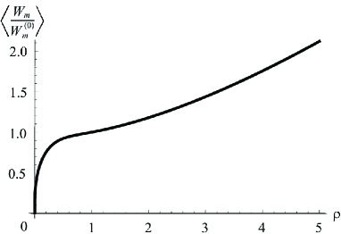
Figure 6: (Color online) Dependence of the average value of the ratio $\,W_{m}/W_{m}^{(0)}$ between the energies of magnetic absorption by a spheroidal metal nanoparticle and a spherical particle with the same volume on the curvature radius ratio $\rho=R_{\bot}/R_{||}$ for the spheroidal particle.

VIII Conclusions

To summarize, a theory describing the dependence of electromagnetic energy absorption by metal nanoparticles on their shape has been developed. Unlike magnetic absorption, electric absorption was found to strongly depend on the nanoparticle shape. This difference is explained by the fact that, in the visible spectral interval, electric absorption is mainly associated with the availability of plasma resonances in nanoparticles. However, the frequencies of plasma resonances, their half-widths and number depend on the nanoparticle shape. Therefore, by changing the parameter $\rho=R_{\bot}/R_{||}$ at a fixed frequency $\omega$ of external irradiation, we can enter into the resonance conditions with the characteristic plasma frequencies of nanoparticles and exit from them. This circumstance is responsible for a drastic dependence of electric absorption on the shape of metal nanoparticles. On the other hand, in the frequency interval where it can be significant [see Eq. (35)], magnetic absorption does not depend on the frequency at all. As one can see from Fig. 5, the dependence of magnetic absorption by nanoparticles on their shape mainly reveals itself in the angular dependence.

We presented the results of our theoretical studies concerning the optical characteristics of an ensemble of spheroidal metal nanoparticle, such as the components of the optical conductivity tensor, the principal values of depolarization tensor components, and the absorption coefficient. The averaged parameters were calculated taking into account the influence of the nanoparticle shape on the depolarization coefficients and the optical conductivity tensor components. The influence of nanoparticle shape on the conductivity was taken into account in the averaging procedure for the first time.

It is well-known that the number of plasma resonances, their frequencies and decrements depend on the nanoparticle shape. In particular, spherical nanoparticles are characterized by one plasma resonance, spheroidal nanoparticles by two, and elliptical ones by three plasma resonances. The result of our calculation testifies that in the case of spheroidal nanoparticle, there are two plasma resonances in a finite frequency interval determined by the input problem parameters. Beyond this interval, only one plasma resonance, $K_{||}\left({\omega,\rho}\right)$, takes place.

A “cap” function (a combination of the “hat” and Gaussian functions) was used to approximate the distribution of nanoparticles over their shape, $P(\rho)$. This model substantially simplifies the solution of a rather complicated problem concerning the influence of the nanoparticle shape non-uniformity over the ensemble on the total absorption coefficient. Furthermore, it was found to be optimal for the qualitative theoretical study of the averaging over the shape spread. The variation of the characteristic parameters of the function $P(\rho)$, such as its half-width and the maximum position, was found to substantially affect the averaged total absorption coefficient $\overline{K\left(\omega\right)}$.

References

- (1) V.V. Klimov, Nanoplasmonics (Fizmatlit, Moscow, 2010) (in Russian).
- (2) P.M. Tomchuk and N.I. Grigorchuk, Phys. Rev. B 73, 155423 (2006).
- (3) E.F. Venger, A.V. Goncharenko, and M.L. Dmytruk, Optics of Small Particles and Dispersion Media (Naukova Dumka, Kyiv, 1999) (in Ukrainian).
- (4) A.V. Goncharenko, E.F. Venger, and S.N. Zavadskii, J. Opt. Soc. Am. B 13, 2392 (1996).
- (5) P.M. Tomchuk and B.P. Tomchuk, Zh. Èksp. Teor. Fiz. 112, 661 (1997).
- (6) R.D. Fedorovich, A.G. Naumovets, and P.M. Tomchuk, Phys. Rep. 328, 73 (2000).
- (7) D.V. Butenko and P.M. Tomchuk, Surf. Sci. 606, 1892 (2012).
- (8) C.F. Boren and D.R. Huffman, Absorption and Scattering of Light by Small Particles (John Wiley and Sons, New York, 1983).
- (9) H.C. van de Hulst, Light Scattering by Small Particles (John Wiley and Sons, New York, 1957).
- (10) L.D. Landau and E.M. Lifshits, Electrodynamics of Continuous Media (Pergamon Press, New York, 1984).
- (11) G. Mie, Beiträge zur Optik trüber Medien, speziell kolloidaler Metallösungen, Ann. Phys. 25, 377 (1908).
- (12) P.M. Tomchuk and D.V. Butenko, Int. J. Mod. Phys. B 31, 1750029 (2017).
- (13) N.I. Grygorchuk and P.M. Tomchuk, Ukr. Fiz. Zh. 51, 921 (2006).
- (14) P.M. Tomchuk and D.V. Butenko, Ukr. Fiz. Zh. 60, 1042 (2015).
- (15) S.L. Sobolev, Some Applications of Functional Analysis in Mathematical Physics (Nauka, Moscow, 1988) (in Russian).
- (16) V.S. Vladimirov, Equations of Mathematical Physics (Nauka, Moscow, 1988) (in Russian).
- (17) V.N. Starkov, M.S. Brodyn, P.M. Tomchuk V.Ya. Gaivoronskyi, and O.Yu. Boyarchuk, Ukr. Fiz. Zh. 60, 602 (2015).
- (18) W. Haiss, N.T.K. Thanh, J. Aveyard, and D.G. Fernig, Anal. Chem. 79, 4215 (2007).
- (19) A. Carrillo-Cazares, N.P. Jiménez-Mancilla, M.A. Luna-Gutiérrez, K. Isaac-Olivé, and M.A. Camacho-López, J. Nanomater. 2017, 3628970 (2017).
- (20) M.I. Grygorchuk and P.M. Tomchuk, J. Phys. Stud. 9, 135 (2005).
- (21) I.A. Kuznetsova, M.E. Lebedev, and A.A. Yushkanov, Zh. Tekhn. Fiz. 85, N 9, 1 (2015).