Continuity properties of folding entropy

Abstract.

The folding entropy is a quantity originally proposed by Ruelle in 1996 during the study of entropy production in the non-equilibrium statistical mechanics [35]. As derived through a limiting process to the non-equilibrium steady state, the continuity of entropy production plays a key role in its physical interpretations. In this paper, we study the continuity of folding entropy for a general (non-invertible) differentiable dynamical system with degeneracy. By introducing a notion called degenerate rate, we prove that on any subset of measures with uniform degenerate rate, the folding entropy, and hence the entropy production, is upper semi-continuous. This extends the upper semi-continuity result in [35] from endomorphisms to all $C^{r}(r>1)$ maps.

We further apply to the one-dimensional setting. In achieving this, an equality between the folding entropy and (Kolmogorov-Sinai) metric entropy, as well as a general dimension formula are established. These admit their own interests. The upper semi-continuity of metric entropy and dimension are then valid when measures with uniform degenerate rate are considered. Moreover, the sharpness of uniform degenerate rate is also investigated by examples in the scope of positive metric (or folding) entropy.

1. Introduction

In the study of non-equilibrium statistical mechanics, the statistical mechanical entropy is exhibited to be persistently pumped out of systems during time evolutions due to the energy or heat exchange with the environment. The numerical experiments in practice indicate that the entropy production is non-negative and usually positive in accordance with the second law of thermodynamics [10, 11, 13], and such phenomenon in the mathematical representations as well has been effectively discussed and justified to certain extent in the stochastic process theory [16, 18, 32, 38, 42].

As a fundamental approach to interpret the thermodynamics, the entropy production theory was especially developed in the framework of dynamical systems [12, 13, 14, 35, 36]. In [35], Ruelle investigated the entropy production in the standard dynamical system $(M,f,\mu)$ where $M$ is a compact Riemannian manifold, the evolution $f:M\to M$ is either a diffeomorphism or a non-invertible differentiable map, and $\mu$ is the non-equilibrium steady state which is normally thought as an SRB (Sinai-Ruelle-Bowen) measure [14, 36]. The entropy production with respect to $\mu$, denoted as $e_{f}(\mu)$, was illustrated through a limiting process in which a quantity called folding entropy naturally arises. Adopting the Shannon-type expression $S(\bar{\rho})=-\int\rho(x)\log\rho(x)dx$ as the statistical mechanical entropy for a probability measure $\bar{\rho}$ with density $\rho,$ the entropy pumped out of the system (to keep the energy fixed due to the non-conservative forces acting on the system) within one-time step is

$$e_{f}(\bar{\rho})=-[S(f\bar{\rho})-S(\bar{\rho})]:=F_{f}(\bar{\rho})-\int_{M}\log|\operatorname{Jac}(D_{x}f)|\rho(x)dx,$$

where $f\bar{\rho}$ denotes the image of $\bar{\rho}$ under $f$. The emerging term $F_{f}(\bar{\rho}),$ called the folding entropy of $\bar{\rho}$, exactly expresses the complexities as $f$ “folds” the different states, according to their $\rho$-weights (or -masses), into a same one. By assuming a general state $\mu$ as the limit of a sequence of absolutely continuous measures with probability densities $\{\rho_{n}\}_{n\geq 1},$ the entropy production with respect to $\mu$ is intuitively given by

$$e_{f}(\mu)=F_{f}(\mu)-\int_{M}\log|\operatorname{Jac}(D_{x}f)|d\mu.$$

Physically considering $\mu$ as an idealization of $\bar{\rho}_{n}$ when $n$ large enough, a natural question is what is the relationship between $e_{f}(\mu)$ and the limiting quantity (if exists) $\lim_{n\to\infty}e_{f}(\bar{\rho}_{n})$? Under some non-degenerate assumptions that essentially requires $f$ to be endomorphism-type, Ruelle [35] showed that the folding entropy is upper semi-continuous and hence

$$e_{f}(\mu)\geq\limsup\nolimits_{n\to\infty}e_{f}(\bar{\rho}_{n}).$$ (1.1)

We remark that when $f$ is a diffeomorphism, the folding entropy is always zero (since no space-folding any more), and the entropy production is simply characterized by the phase volume contraction $-\int\log|\operatorname{Jac}(D_{x}f)|d\mu.$ This relation was earlier pointed in the discussion of more concrete non-equilibrium molecular dynamics models [9, 10, 15] and theoretically revealed in [1, 13]. In this situation, the equality in the limiting process (1.1) naturally holds due to the continuity of the function $\log|\operatorname{Jac}(D_{x}f)|$.

By the physical motivations to general situations, the results in [35] were conjecturally extended and a unified presentation was suggested. The further progress actually depends on the study in the ergodic theory of differentiable dynamical systems. For a general (non-invertible) system beyond endomorphism, the analysis difficulty of entropy production is in the handling of the possible accumulation of “foldings” due to the degeneracy (even with zero measure) in the approximation process. In this paper, we assume, standardly, that $f$ is a $C^{r}(r>1)$ map on a compact Riemannian manifold $M$. Our main goal is to explore the mechanism for the upper semi-continuity of folding entropy. By introducing a notion called degenerate rate which captures the complexity arising near the degenerate set $\Sigma_{f}:=\{x\in M:\operatorname{Jac}(D_{x}f)=0\}$, we shall establish the upper semi-continuity of folding entropy on any set of measures with uniform degenerate rate. This thus justifies (1.1) in the limiting process.

1.1. Folding entropy and degenerate rate

We begin with the precise definition of folding entropy. Denote by $\operatorname{\mathcal{P}}(M)$ the set of all Borel probability measures on $M$. For $\mu\in\operatorname{\mathcal{P}}(M),$ the folding entropy $F_{f}(\mu)$ is a conditional entropy measuring the complexities of the $\mu$-weighted preimages of $f.$ More specifically, denote $f^{-1}\epsilon=\big{\{}\{f^{-1}x\}\big{\}}_{x\in M}$ as the preimage partition of $f$ with $\epsilon:=\{\{x\}\}_{x\in M}$ being the partition into single points. Then the folding entropy of $f$ with respect to $\mu$ is the conditional entropy of $\epsilon$ relative to $f^{-1}\epsilon$:

$$F_{f}(\mu)=H_{\mu}(\epsilon|f^{-1}\operatorname{\epsilon})=\displaystyle\int_{M}H_{\tilde{\mu}_{x}}(\epsilon)d(f\mu),$$

where $\{\tilde{\mu}_{x}\}$ is the family of conditional measure of $\mu$ disintegrated along the preimage sets $\{f^{-1}x\}$.

Despite for its seemingly abstract form, the folding entropy is in practice rather intuitive; see Figure 1(A). We see that if there are only finitely many preimage branches, say $N,$ then the folding entropy is always bounded by $\log N$ since $H(\tilde{\mu}_{x})\leq\log N$, and the equality is achieved if all the $N$ preimages are equally $\mu$-weighted. In particular, if $f$ is a diffeomorphism, then $N=1$ and hence $F_{f}(\mu)=0$. A simple but illuminating example is to consider $M=\operatorname{\mathbb{S}}^{1}$ and $f:x\mapsto Nx$ (mod 1) for $N\in\mathbb{N}.$ In this example, since $f$ “evenly” expands the state space $\operatorname{\mathbb{S}}^{1}$, the folding entropy with respect to the Lebesgue measure (which is also an SRB measure) is $F_{f}(\mathcal{L}eb)=\log N.$ Generalizing a bit more in the situation of two preimage pieces, consider $f(x)=px$ for $x\in[0,1/p)$ and $f(x)=\frac{p}{p-1}(1-x)$ for $x\in[1/p,1)$, where $1<p\neq 2$. The subintervals $[0,1/p)$ and $[1/p,1)$ are stretched by $f$ in different scales. Still, the Lebesgue measure is an SRB measure, however the folding entropy $F_{f}(\mathcal{L}eb)=-\frac{1}{p}\log\frac{1}{p}-\frac{p-1}{p}\log\frac{p-1}{p}<\log 2.$

As a consequence of physically motivated and mathematically intuitive role played by the folding entropy, a folding-type entropy inequality on the backward process was simultaneously revealed in [35] in contrast with the forward evolution. To be specific, for a $C^{r}(r>1)$ map $f$ on a compact Riemannian manifold $M$ and an $f$-invariant measure $\mu,$ the folding-type Ruelle inequality reads as

$$h_{\mu}(f)\leq F_{f}(\mu)-\int_{M}\sum_{\lambda_{i}(f,x)<0}\lambda_{i}(f,x)d\mu,$$ (1.2)

where $\lambda_{i}(f,x)$ denote the Lyapunov exponents, existing for $\mu$-a.e. $x\in M$ by the Oseledec theorem [29]. The inequality (1.2) was conjectured in [35] providing an approach to the non-negativity of entropy production and was mathematically rigorously proved by Liu [24] for $C^{r}(r>1)$ maps under some polynomial-like degeneracy conditions, and then by the authors [23] for all $C^{r}(r>1)$ maps. We would like to mention that in the classical Margulis-Ruelle inequality [34], the RHS is simply the sum of positive Lyapunov exponents [34]. With respect to the backward process, however, since one trajectory may split into many branches, the folding entropy appears as a characterization of this “global” expansion in terms of branches, while the “local” expansions inside each branch are captured by the Lyapunov exponents.

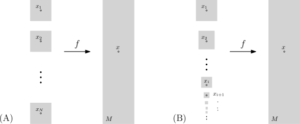
Figure 1. (A) There are $N$ branches containing the $N$ preimages, $x_{1},\cdots,x_{N},$ of a typical $x\in M,$ i.e., $f(x_{1})=\cdots=f(x_{N})=x.$  (B) There are countably many branches containing the preimages, $x_{1},\cdots,x_{i},\cdots,$ of a typical $x\in M.$ The accumulation happens near the degenerate set.

In [35], it was shown that under the “endomorphism-type” assumptions, the folding entropy varies in an upper semi-continuous way. In this situation, a single coarse-grained partition alone can exhaust all the complexities in the folding process. However, this does not work in general, especially when arbitrarily many preimage branches accumulate around the degenerate set; see Figure 1(B). A general influence mechanism by the degeneracy for systems beyond endomorphisms remains unknown yet. The main goal of this paper is to develop a such mechanism. To achieve this, we introduce a notion called degenerate rate to capture the emerging complexities in the refining coarse-graining process. Take firstly a decreasing sequence of open neighborhoods of $\Sigma_{f},$ denoted by $\mathcal{V}=\{V_{m}\}_{m\geq 1},$ such that

$$d_{H}(V_{m},\Sigma_{f})\to 0,\quad m\to\infty,$$ (1.3)

where $d_{H}$ denotes the Hausdorff distance. Let $\bar{\eta}=\{\eta_{m}\}_{m\geq 1}$ be any sequence of positive real numbers approaching to zero. Given $\mu\in\operatorname{\mathcal{P}}(M),$ $f$ is said to admit degenerate rate $\bar{\eta}$ with respect to $\mu$ if

$$\Big{|}\int_{V_{m}}\log|\operatorname{Jac}(D_{x}f)|d\mu\Big{|}\leq\eta_{m},\quad\forall m\geq 1.$$

In the definition, $\bar{\eta}$ actually characterizes the level of complexities arising near $\Sigma_{f}$, i.e., how $|\operatorname{Jac}(D_{x}f)|$ diminishes on the shrinking domains around $\Sigma_{f}$. It is well-defined for any $\mu\in\operatorname{\mathcal{P}}(M)$ satisfying the integrable condition

$$\Big{|}\int\log|\operatorname{Jac}(D_{x}f)|d\mu\Big{|}<\infty.$$ (1.4)

We will focus on the probability measures with a uniform degenerate rate. Define

$$\operatorname{\mathcal{P}}_{\bar{\eta}}(f):=\Big{\{}\nu\in\operatorname{\mathcal{P}}(M):\Big{|}\int_{V_{m}}\log|\operatorname{Jac}(D_{x}f)|d\mu\Big{|}\leq\eta_{m},\,\,\forall m\geq 1\Big{\}},$$

i.e., $\operatorname{\mathcal{P}}_{\bar{\eta}}(f)$ collects all the probability measures with the degenerate rate $\bar{\eta}$. Note that any $\mu\in\operatorname{\mathcal{P}}_{\bar{\eta}}(f)$, $\mu(\Sigma_{f})=0$ holds automatically. Before proceeding to the theorems, we give two remarks about $\operatorname{\mathcal{P}}_{\bar{\eta}}(f)$:

(i) $\operatorname{\mathcal{P}}_{\bar{\eta}}(f)$ is a closed subset of $\operatorname{\mathcal{P}}(M)$ in the weak^∗-topology. To see this, let $\{\mu_{i}\}_{i\geq 1}$ be a sequence of measures in $\operatorname{\mathcal{P}}_{\bar{\eta}}(f)$ satisfying $\lim_{i\to\infty}\mu_{i}=\mu$. Without loss of generality, we assume that $|\operatorname{Jac}(D_{x}f)|\big{|}_{V_{m}}<1$ for all $m\geq 1.$ Then for any $s>m$, $|\int_{V_{m}\setminus V_{s}}\log|\operatorname{Jac}(D_{x}f)|d\mu_{i}|\leq\eta_{m}.$ Hence,

$$\Big{|}\int_{V_{m}\setminus V_{s}}\log|\operatorname{Jac}(D_{x}f)|d\mu\Big{|}=\lim_{i\to\infty}\Big{|}\int_{V_{m}\setminus V_{s}}\log|\operatorname{Jac}(D_{x}f)|d\mu_{i}\Big{|}\leq\eta_{m}.$$

This, together with $\mu(\Sigma_{f})=0,$ yields

$$\Big{|}\int_{V_{m}}\log|\operatorname{Jac}(D_{x}f)|d\mu\Big{|}\leq\eta_{m},\quad\forall m\geq 1.$$

That is, $\mu\in\operatorname{\mathcal{P}}_{\bar{\eta}}(f).$

(ii) The uniform degenerate rate is independent on the choice of $\mathcal{V}=\{V_{m}\}_{m\geq 1}$. Actually, for any two sequences of neighborhoods of $\Sigma_{f},$ $\mathcal{V}^{(i)}=\{V_{m}^{(i)}\}_{m\geq 1}$ $(i=1,2)$ satisfying (1.3), the associated tails

$$\Big{\{}\Big{|}\int_{V_{m}^{(i)}}\log|\operatorname{Jac}(D_{x}f)|d\mu\Big{|}\Big{\}}_{m\geq 1}\quad(i=1,2),$$

are uniformly equivalent, i.e., for any $\gamma>0$ and $m_{1}\geq 1,$ there exists $m_{2}>0$ such that

$$\Big{|}\int_{V_{m}^{(2)}}\log|\operatorname{Jac}(D_{x}f)|d\mu\Big{|}<\Big{|}\int_{V_{m_{1}}^{(1)}}\log|\operatorname{Jac}(D_{x}f)|d\mu\Big{|}+\gamma,\quad\forall m\geq m_{2},$$

and vice versa. Henceforth, we fix a decreasing sequence $\mathcal{V}=\{V_{m}\}_{m\geq 1}$ satisfying (1.3). By the variation of the sequence $\bar{\eta}=\{\eta_{m}\}_{m\geq 1}$ with zero limit, all the settings of uniform degenerate rate will then be exhausted.

For a general $C^{r}(r>1)$ system, the upper semi-continuity of folding entropy is established when measures with uniform degenerate rates are considered.

Theorem 1.1.

Let $f$ be a $C^{r}(r>1)$ map on a compact Riemannian manifold $M.$ Then the folding entropy

$$\mu\mapsto F_{f}(\mu)$$

is upper semi-continuous on $\operatorname{\mathcal{P}}_{\bar{\eta}}(f).$

Note that on $\operatorname{\mathcal{P}}_{\bar{\eta}}(f),$ the map $\mu\mapsto\int\log|\operatorname{Jac}(D_{x}f)|d\mu$ is continuous because the singular part, i.e., the integral on the neighborhood of $\Sigma_{f}$, is uniformly controlled. Thus, Theorem 1.1 directly yields the upper semi-continuity of the entropy production.

Corollary 1.2.

Let $f$ be a $C^{r}(r>1)$ map on a compact Riemannian manifold $M.$ Let $\{\mu_{n}\}_{n\geq 1}\subseteq\operatorname{\mathcal{P}}_{\bar{\eta}}(f)$ be a sequence of measures such that $\lim_{n\to\infty}\mu_{n}=\mu.$ Then it holds that

$$e_{f}(\mu)\geq\limsup\nolimits_{n\to\infty}e_{f}(\mu_{n}).$$

1.2. Applications to interval maps

As is well-known that for a measurable dynamical system, the (Kolmogorov-Sinai) metric entropy measures the complexities (or uncertainties) produced during the dynamical evolutions. Among the various properties of metric entropy that has been well studied, the upper semi-continuity has drawn much attention as it plays a key role for the existence of equilibrium states [3, 39]. In the context of interval maps, we will establish an equality relation between folding entropy and metric entropy; see Theorem 4.1. Then as an application of Theorem 1.1, the upper semi-continuity property of the latter one is obtained when invariant measures with uniform degenerate rates are considered. Henceforth, for an interval map $f$, let $\operatorname{\mathcal{M}}_{inv}(f)$ be the set of all $f$-invariant Borel probability measures, and still, $\bar{\eta}=\{\eta_{m}\}_{m\geq 1}$ be the any sequence of positive real numbers approaching to zero. Then

$$\mathcal{M}_{\bar{\eta},inv}(f):=\operatorname{\mathcal{P}}_{\bar{\eta}}(f)\cap\mathcal{M}_{inv}(f)$$

denotes the set of all $f$-invariant Borel probability measures with uniform degenerate rate $\bar{\eta}$.

Theorem 1.3.

Let $f$ be a $C^{r}(r>1)$ interval map. Then the metric entropy

$$\mu\mapsto h_{\mu}(f)$$

is upper semi-continuous on $\mathcal{M}_{\bar{\eta},inv}(f).$

Remark: In the theory of differentiable dynamical systems, the hyperbolicity and the smoothness are two basic mechanisms leading to the upper semi-continuity of metric entropy. On the one hand, for all $C^{\infty}$ systems, the upper semi-continuity of metric (or topological entropy) always holds true [28, 40]. In fact, $C^{\infty}$ smoothness brings about the uniform control of degeneracy and hence foldings, which, as already shown by various examples [6, 26, 27, 37], can be destroyed if only finite smoothness is considered. On the other hand, for systems with some hyperbolicity, e.g., the uniformly hyperbolic systems [2], the partially hyperbolic systems with one dimensional center [7, 8], and the diffeomorphisms away from tangencies [22], the upper semi-continuity property of metric entropy is shown to be valid. In the particular setting of non-uniformly hyperbolic systems, Newhouse proposed hyperbolic rate to characterize the level of hyperbolicity for invariant measures, and proved the upper semi-continuity of metric entropy on the set with uniform hyperbolic rate [28]. The degenerate rate in this paper for the studying of folding entropy, without any requirements of measure preserving and hyperbolicity, plays an analogous role of the hyperbolic rate from the view of the degeneracy.

Besides the entropy, dimension is another intrinsic characteristic of complexity in the dynamical theory. For a differentiable dynamical system, the interrelation among the various dynamical quantities has been intensively investigated [19, 21, 30, 34, 41]. In particular, for an interval map $f$ and an ergodic $f$-invariant Borel probability measure $\mu,$ the following formula

$$h_{\mu}(f)=\lambda^{+}(\mu)\operatorname{dim}(\mu)$$ (1.5)

was established in [19] under certain assumptions on the degeneracy, where $\lambda^{+}(\mu)=\max\{\lambda(\mu),0\}$ is the positive part of the Lyapunov exponent $\lambda(\mu)$ of $\mu$. In Section 4, by developing an integrable version of the Brin-Katok formula, we show the validity of (1.5) for any $C^{r}(r>1)$ interval map $f$ and hyperbolic (i.e., $\lambda(\mu)\neq 0$) ergodic Borel probability measure $\mu$; see Theorem 4.2. We emphasize that the hyperbolicity of measure is necessary here, since the dimension may not exist for non-hyperbolic measures in general [17, 20]. As a consequence of Theorem 1.3, we obtain the upper semi-continuity of dimension at all hyperbolic measures on the set of ergodic measures with uniform degenerate rate. For convenience, write

$$\mathcal{M}_{\bar{\eta},erg}(f)=\mathcal{P}_{\bar{\eta}}(f)\cap\mathcal{M}_{erg}(f),$$

where $\operatorname{\mathcal{M}}_{erg}(f)$ denotes the set of all ergodic $f$-invariant Borel probability measures.

Theorem 1.4.

Let $f$ be a $C^{r}(r>1)$ interval map. Then the dimension

$$\mu\mapsto\operatorname{dim}(\mu)$$

is upper semi-continuous at all hyperbolic measures in $\mathcal{M}_{\bar{\eta},erg}(f).$

1.3. Sharpness of the uniform degenerate rate condition

For the previous known examples concerning the loss of upper semi-continuity of metric entropy, the ergodic measures at which the upper semi-continuity fails are all atomic and hence admit zero metric entropy (see, for instance, [6, 27, 37]). Note that the positivity of metric entropy for an ergodic measure implies that the hyperbolicity holds in a nontrivial full-measure set (due to the Margulis-Ruelle inequality [34] and ergodicity). In the consideration that the hyperbolicity has been a possible approach to the upper semi-continuity of metric entropy [2], there arises a natural question suggested by Burguet in [5]

Question: Is the metric entropy of a $C^{r}$ ($r>1$) interval map upper semi-continuous at ergodic measures with positive entropy?

Taking into account the approximation of measures by the generic orbits, we will construct a type of modified examples in Section 5 for which the loss of upper semi-continuity of metric entropy occurs at a non-atomic ergodic measure, say $\mu,$ with positive entropy. The defect of upper semi-continuity of metric entropy at $\mu$ follows from the infinite “foldings” around a homoclinic tangency whose images in average converging to $\mu;$ see Figure 5. The approximation is realized by taking some generic point of $\mu,$ say $x_{0}$, and then elaborately choose a sequence of (ergodic) measures whose generic points follow the orbit of $x_{0}$ with large frequency, but do NOT admit a uniform degenerate rate. This indicates that in the setting of differentiable systems (with degeneracy), the uniform degenerate rate serves as an essential condition for the upper semi-continuity of folding entropy.

Theorem 1.5.

For any $1<r<\infty$, there exist $C^{r}$ interval maps admitting ergodic measures with positive entropy as the non upper semi-continuity points of the metric (or folding) entropy.

This paper is organized as follows. In Section 2, we review the basic notions in the ergodic and entropy theory that will be used throughout this paper. In Section 3, we prove Theorem 1.1. In Section 4, we discuss the applications to the one-dimensional setting. An entropy formula (Theorem 4.1) and a dimension formula (Theorem 4.2) are established for all $C^{r}(r>1)$ interval maps. Theorem 1.3 and Theorem 1.4 then follows almost immediately. In Section 5, we concretely construct a type of modified interval maps for which a typical failing mechanism of the upper semi-continuity of metric entropy at an ergodic measure with positive entropy is developed. The sharpness of the condition about the uniform degenerate rate in Theorem 1.1 and Theorem 1.3 is also illustrated.

2. Preliminaries

In this section, we recall some basic notions and facts in the ergodic and entropy theory that will be used in the later discussions. Readers may refer to [33, 39] for more details.

- Invariant measure, partition and entropy. Let $X$ be a compact metric space with the Borel $\sigma$-algebra $\mathcal{B}$, and $f:X\to X$ be a measurable transformation. Recall as in the introduction that $\operatorname{\mathcal{P}}(X)$ denotes the set of all Borel probability measures on $X$ endowed with the weak^∗-topology, i.e., $\mu_{n}\to\mu$ in $\operatorname{\mathcal{P}}(X)$ if and only if for any continuous function $\varphi$, $\int\varphi d\mu_{n}\to\int\varphi d\mu$ as $n\to\infty.$ For $\mu\in\operatorname{\mathcal{P}}(X),$ the image of $\mu$ under $f$ is given by $f\mu(B)=\mu(f^{-1}B),\forall B\in\operatorname{\mathcal{B}},$ and $\mu$ is said to be $f$-invariant if $f\mu=\mu.$ Denote by $\operatorname{\mathcal{M}}_{inv}(f)$ the set of all $f$-invariant Borel probability measures.

A partition $\xi=\{A_{\operatorname{\alpha}}\}_{\operatorname{\alpha}\in\mathscr{A}}$ of $X$ is a collection of disjoint elements of $\operatorname{\mathcal{B}}$ such that $\cup_{\alpha\in\mathscr{A}}A_{\operatorname{\alpha}}=X.$ In particular, $\xi$ is called finite if the cardinality $\#\mathscr{A}<\infty.$ Given two partitions $\xi=\{A_{\alpha}\}_{\alpha\in\mathscr{A}}$ and $\zeta=\{C_{\gamma}\}_{\operatorname{\gamma}\in\mathscr{C}},$ the join of $\xi$ and $\zeta$ is a partition of $X$, denoted as $\xi\vee\zeta,$ such that

$$\xi\vee\zeta=\{A_{\alpha}\cap C_{\gamma}\}_{\alpha\in\mathscr{A},\gamma\in\mathscr{C}}.$$

If $\xi\vee\zeta=\zeta,$ i.e., each element of $\xi$ is a union of elements of $\zeta,$ then we call $\zeta$ is a refinement of $\xi,$ and write $\xi\preceq\zeta.$ A sequence of partitions $\{\xi_{n}\}_{n\geq 1}$ is said to be refining (or increasing) if $\xi_{1}\preceq\xi_{2}\preceq\cdots\preceq\xi_{n}\preceq\cdots.$

Given $\mu\in\operatorname{\mathcal{P}}(X)$ and a finite partition $\xi$ of $X,$ the entropy of $\xi$ with respect to $\mu$ is

$$H_{\mu}(\xi)=\displaystyle\int_{X}-\log\mu(\xi(x))d\mu(x),$$

where $\xi(x)$ denotes the element of $\xi$ containing $x.$ For any two finite partitions $\xi$ and $\zeta$, the conditional entropy of $\xi$ given $\zeta$ is

$$H_{\mu}(\xi|\zeta)=\sum_{C\in\zeta}\mu(C)H_{\mu_{C}}(\xi|_{C})=\sum_{A\in\xi,C\in\zeta}-\mu(A\cap C)\log\Big{(}\dfrac{\mu(A\cap C)}{\mu(C)}\Big{)}$$

where $\mu_{C}(A):=\mu(A\cap C)/\mu(C)$ is the conditional measure of $A$ given $C,$ and $\xi|_{C}$ denotes the partition $\xi$ restricted on $C.$ For any $\mu\in\operatorname{\mathcal{M}}_{inv}(f)$, the metric entropy of $f$ with respect to $\mu$ and $\xi$ is

$$h_{\mu}(f,\xi)=\lim_{n\to\infty}H_{\mu}(\xi|\bigvee_{i=1}^{n}f^{-i}\xi)=\inf_{n\geq 1}H_{\mu}(\xi|\bigvee_{i=1}^{n}f^{-i}\xi),$$ (2.1)

and the metric entropy of $f$ with respect to $\mu$ is

$$h_{\mu}(f)=\sup_{\xi}h_{\mu}(f,\xi),$$

where the supremum is taken over all finite partitions of $X.$

We remark that the entropy and conditional entropy can be defined in the more general setting where $(X,\operatorname{\mathcal{B}},\mu)$ is a Lebesgue space and $\xi,\zeta$ are measurable partitions. The folding entropy is a particular type of conditional entropy in this setting with $\xi$ and $\zeta$ be chosen as $\operatorname{\epsilon}$ and $f^{-1}\operatorname{\epsilon},$ respectively. See [33] for more discussions on this.

In the estimation of entropy, a basically important function from the information theory is as follows:

$$\phi(x)=\begin{cases}-x\log x,&x\in(0,1];\\ 0,&x=0.\end{cases}$$

As a simple result of the concavity of $\phi$, the following proposition will be use several times in section 3.

Proposition 2.1.

Let $\{p_{i}\}_{i=1}^{n}$ be such that $\sum_{i=1}^{n}p_{i}=1$ and $p_{i}\geq 0,1\leq i\leq n$, and $\{x_{i}\}_{i=1}^{n}\subset[0,1]$. Then

$$\sum_{i=1}^{n}p_{i}\phi(x_{i})\leq\phi(\sum_{i=1}^{n}p_{i}x_{i}).$$

In particular, $\sum_{i=1}^{n}\phi(p_{i})\leq\log n.$

- Dimension of a measure. For the compact metric space $X$ with distance $d$, given any finite Borel measure $\mu$, for $\mu$-a.e. $x\in X$, the lower and upper local dimension are respectively defined as

$$\underline{\operatorname{dim}}(x)=\liminf_{\delta\to 0}\frac{\log\mu(B(x,\delta))}{\log\delta},\quad\overline{\operatorname{dim}}(x)=\limsup_{\delta\to 0}\frac{\log\mu(B(x,\delta))}{\log\delta},$$

where $B(x,\delta)=\{y\in X:d(y,x)<\delta\}.$ The measure $\mu$ is said to have local dimension at $x$ if $\underline{\operatorname{dim}}(x)=\overline{\operatorname{dim}}(x).$ For a subset $Y\subset X$ and a number $t>0$, the $t$-Hausdorff measure of $Y$ is defined by

$$m_{H}(Y,t)=\lim_{\operatorname{\varepsilon}\to 0}\inf_{\mathcal{U}}\sum\nolimits_{U\in\mathcal{U}}\operatorname{diam}^{t}(U),$$

where the infimum is taken over all finite or countable coverings $\mathcal{U}$ of $Y$ by open sets with $\operatorname{diam}(\mathcal{U})\leq\operatorname{\varepsilon}$. The Hausdorff dimension of $Y$ and then of $\mu$ are respectively defined as

$$\operatorname{dim}_{H}(Y)=\inf\big{\{}t:m_{H}(Y,t)=0\big{\}}=\sup\big{\{}t:m_{H}(Y,t)=\infty\big{\}},$$

$$\operatorname{dim}_{H}(\mu)=\inf\big{\{}\operatorname{dim}_{H}(Y):\mu(Y)=1\big{\}}.$$

The following classical result says that under standard conditions, the local dimension exists and coincides with the Hausdorff dimension.

Proposition 2.2 (Young [41]).

Let $X$ be a compact separable metric space of finite topological dimension and $\mu$ be a finite Borel measure on $X$ satisfying

$$\underline{\operatorname{dim}}(x)=\overline{\operatorname{dim}}(x)=D,\quad\mu{\text{-a.e.}}\ x\in X.$$ (2.2)

Then $\operatorname{dim}_{H}(\mu)=D.$

Any measure $\mu$ satisfying (2.2) is said to be exact dimensional with the common value denoted by $\operatorname{dim}(\mu).$

3. upper semi-continuity of folding entropy

In this section, we prove Theorem 1.1. Throughout, let $f$ be a $C^{r}(r>1)$ map on a compact Riemannian manifold $M.$ Before proceeding to the proof, we would like to note that the basic idea in the handling of the degeneracy in the proof, though are based on that in [23] with some further refining estimations, are more clearly explained and revealed here.

3.1. Construction of refining partitions

For convenience of analysis, we embed $M$ into an Euclidean space $\mathbb{R}^{N}.$ Then, one can find tubular neighborhoods ${T_{1}}\subset T_{2}$ of $M$ in $\mathbb{R}^{N},$ and a $C^{r}$ extension $g$ of $f$ from $T_{1}$ to $T_{2}$ such that $g^{-1}(\overline{T}_{1}))\subset T_{1}$ and $M=\cap_{n\in\mathbb{N}}\,g^{-n}(T_{1})$. Without confusion, we still write $g|_{T_{1}}$ as $f$ for simplicity. Let $\alpha=\min\{r-1,1\}.$ Then the derivative of $f$, denoted as $Df,$ is $\alpha$-Hölder continuous, i.e, there exists $K>1$ such that

$$\|D_{x}f-D_{y}f\|\leq\,Kd(x,y)^{\alpha},\quad\forall\,x,y\in T_{1}.$$ (3.1)

To approximate the folding entropy, we shall use a sequence of refining finite partitions to approximate the measurable partitions $\{\operatorname{\epsilon}|_{f^{-1}\operatorname{\epsilon}(x)}\}_{x\in T_{1}}$. To begin with, for each $k\in\operatorname{\mathbb{N}},$ define the partition $\Gamma_{k}$ of $\operatorname{\mathbb{R}}^{N}$ as

$$\Gamma_{k}=\Big{\{}(\frac{q_{1}}{2^{k}},\frac{q_{1}+1}{2^{k}})\overbrace{\times\cdots\times}^{N}(\frac{q_{N}}{2^{k}},\frac{q_{N}+1}{2^{k}})~{}:~{}q_{1},\cdots,q_{N}\in\mathbb{Z}\Big{\}}.$$

Plainly, $\Gamma_{1}\preceq\cdots\preceq\operatorname{\Gamma}_{k}\preceq\cdots.$ Since $f$ only acts on $T_{1},$ henceforth, by $\Gamma_{k}$ we mean $\Gamma_{k}|_{T_{1}}.$ Note that there exists a constant $C_{1}>0$, independent of $k,N$, such that

$$\#\big{\{}A\in\Gamma_{k}:A\cap T_{1}\neq\emptyset\big{\}}\leq C_{1}2^{kN},\quad\forall\,k\in\mathbb{N}.$$ (3.2)

Intuitively, to approximate the $f$-inverse partition $f^{-1}\operatorname{\epsilon},$ we need to consider the “pull-back” of $\{\Gamma_{k}\}.$ In achieving this, we have to deal with the degeneracy of $f$. Given any $\operatorname{\varepsilon}>0$, define

$$U_{\operatorname{\varepsilon}}=\big{\{}x\in T_{1}:m(D_{x}f)<\operatorname{\varepsilon}\big{\}},\quad G_{\operatorname{\varepsilon}}=\big{\{}x\in T_{1}:m(D_{x}f)\geq\operatorname{\varepsilon}\big{\}},$$

where $m(\Phi):=\inf_{\|z\|=1}\|\Phi(z)\|$ denotes the small norm of a linear operator $\Phi$. By (3.1), if take $r_{\operatorname{\varepsilon}}=(\frac{\operatorname{\varepsilon}^{2}}{4K})^{\frac{1}{\alpha}},$ we have $m(D_{x}f)>\frac{\operatorname{\varepsilon}}{2},\forall x\in G_{\operatorname{\varepsilon}}.$ For each $k\in\operatorname{\mathbb{N}},$ let $\operatorname{\varepsilon}_{k}=\operatorname{\varepsilon}_{0}2^{-k\beta}$ with $\beta=\frac{\alpha}{2+\alpha}$ and $\operatorname{\varepsilon}_{0}=(2(4K)^{\frac{1}{\alpha}}\sqrt{N})^{\beta}.$ Then corresponding to each $\operatorname{\Gamma}_{k}$, $k\in\operatorname{\mathbb{N}},$

$$f(B(x,r_{\operatorname{\varepsilon}_{k}}))\supseteq\Gamma_{k}(fx),\quad\forall x\in G_{\operatorname{\varepsilon}_{k}},$$ (3.3)

where $\Gamma_{k}(fx)$ denotes the element of $\Gamma_{k}$ containing $fx.$ Obviously, $\{U_{\operatorname{\varepsilon}_{k}}\}$ is a sequence of decreasing neighborhoods of $\Sigma_{f}$ as $k\to\infty.$

Now, for each $P\in\Gamma_{k}$, denote $P^{-1,c}$ as the set of all the connected components of $f^{-1}P.$ Separating and collecting the components “near” $\Sigma_{f}$, let

$$B_{k}=\bigcup_{P\in\Gamma_{k}}\,\,\bigcup_{\begin{subarray}{c}Q\in P^{-1,c},\\ Q\cap U_{\operatorname{\varepsilon}_{k}}\neq\emptyset\end{subarray}}\,\,Q.$$

Obviously, $B_{k}\supset U_{\operatorname{\varepsilon}_{k}};$ see Figure 2(A). The following lemma shows that $B_{k}$ is contained in certain $U_{\delta}$ for $\delta$ being the same order as $\operatorname{\varepsilon}_{k}.$

Lemma 3.1.

For any $k\geq 1,$

$$B_{k}\subset U_{C_{2}2^{-k\beta}},$$

for some constant $C_{2}>0$ independent of $k,\beta.$

Proof.

We claim that for any $Q\in P^{-1,c},$ where $P\in\operatorname{\Gamma}_{k},$ such that $Q\cap U_{\operatorname{\varepsilon}_{k}}\neq\varnothing,$ it holds that

$$B(x,r_{\operatorname{\varepsilon}_{k}})\cap U_{\operatorname{\varepsilon}_{k}}\neq\varnothing,\quad\forall x\in Q.$$ (3.4)

For otherwise, if for some $x_{0}\in Q$ such that $B(x_{0},r_{\operatorname{\varepsilon}_{k}})\cap U_{\operatorname{\varepsilon}_{k}}=\varnothing,$ then by (3.3), $B(x_{0},r_{\operatorname{\varepsilon}_{k}})$ contains certain preimage component of $f^{-1}\big{(}\operatorname{\Gamma}_{k}(fx_{0})\big{)},$ say $Q_{0},$ such that $x_{0}\in Q_{0}$. Hence, $Q=Q_{0}.$ This contradicts with $Q\cap U_{\operatorname{\varepsilon}_{k}}\neq\varnothing.$

Now, together with (3.1), (3.4) yields

$$m(D_{x}f)\leq\operatorname{\varepsilon}_{k}+Kr_{\operatorname{\varepsilon}_{k}}^{\alpha}\leq C_{2}2^{-k\beta},\quad\forall x\in B_{k},$$

for some constant $C_{2}>0.$ Hence, $B_{k}\subset U_{C_{2}2^{-k\beta}}.$ ∎

Define the pullback partition of $\Gamma_{k},$ denoted by $\Gamma_{k}^{-1,c}$, as

$$\Gamma^{-1,c}_{k}:=\{B_{k}\}\bigcup_{P\in\Gamma_{k}}\{Q\in P^{-1,c}:Q\cap U_{\operatorname{\varepsilon}_{k}}=\emptyset\}.$$

We note that $\operatorname{\Gamma}^{-1,c}_{k}$ is a finite approximation of the measurable partition $\operatorname{\epsilon}|_{f^{-1}\operatorname{\epsilon}}$ in such a way that all the preimages away from $\Sigma_{f}$ are separated by different components $Q\in P^{-1,c},$ while those close to $\Sigma_{f}$ are collected by $B_{k};$ see Figure 2(B). We call $B_{k}$ the degenerate component of $\operatorname{\Gamma}_{k}^{-1,c}.$ In the following, we shall use the conditional entropy $H_{\mu}(\operatorname{\Gamma}_{k}^{-1,c}|f^{-1}\operatorname{\Gamma}_{k})$ to approximate the folding entropy through the refining process $k\to\infty.$

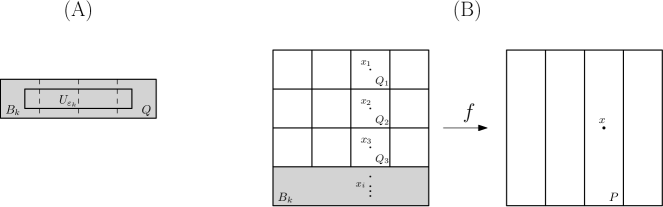
Figure 2. (A) The degenerate component $B_{k}$ consists of all the components $Q\in\operatorname{\Gamma}_{k}$ (denoted by dashed line) that intersect with $U_{\operatorname{\varepsilon}_{k}}.$ (B) The left panel denotes the pullback partition $\operatorname{\Gamma}_{k}^{-1,c};$ the right panel denotes the partition $\operatorname{\Gamma}_{k}.$ For a typical $P\in\Gamma_{k},$ $x\in P,$ the preimages of $x,$ $x_{i}(i=1,2,3)$ lie in the different components $Q_{i}\in P^{-1,c}(i=1,2,3).$ The other preimages $x_{i}(i=4,\cdots)$ are all collected by the degenerate component $B_{k}\in\operatorname{\Gamma}_{k}^{-1,c}.$

3.2. Approximating the folding entropy

Up to the end of this section, we consider measures $\nu\in\operatorname{\mathcal{P}}(M)$ for certain degenerate rate $\bar{\eta}.$ Then it holds that

$$\Big{|}\int\log|\operatorname{Jac}(D_{x}f)|d\nu(x)\Big{|}<\infty.$$

Hence, $\nu(B_{k})\to 0$ as $k\to\infty.$ By construction, for $\nu$-a.e. $x,$ $\Gamma^{-1,c}_{k}$ is increasing to $\epsilon|_{(f^{-1}\operatorname{\epsilon})(x)}$ as $k\to\infty$. Therefore,

$$F_{f}(\nu) = \lim_{k\to+\infty}H_{\mu}(\Gamma^{-1,c}_{k}\mid f^{-1}\epsilon)$$ (3.5)

$$\leq \limsup_{k\to+\infty}H_{\mu}(\Gamma^{-1,c}_{k}\mid f^{-1}\Gamma_{k})$$

$$= \limsup_{k\to\infty}\sum_{P\in\Gamma_{k}}\sum_{Q\in\Gamma^{-1,c}_{k}}-\nu(Q\cap f^{-1}P)\log\Big{(}\frac{\nu(Q\cap f^{-1}P)}{\nu(f^{-1}P)}\Big{)}.$$

For the (upper semi-)continuity analysis later, we shall split the summation in (3.5) into two parts to collect the complexities near and away from $\Sigma_{f},$ respectively. First, we note that for any $Q\in\operatorname{\Gamma}_{k}^{-1,c},$ either $Q=B_{k},$ or $Q\cap B_{k}=\varnothing,$ where in the latter case, $f|_{Q}$ is a diffeomorphism such that $fQ=P$ for certain $P\in\operatorname{\Gamma}_{k}.$ Now according to whether $Q$ equal to $B_{k}$ or not, the RHS of (3.5) is split into two parts:

$$\Delta_{k}^{(1)}(\nu) = \sum_{P\in\Gamma_{k}}-\nu(B_{k}\cap f^{-1}P)\log\Big{(}\dfrac{\nu(B_{k}\cap f^{-1}P)}{\nu(f^{-1}P)}\Big{)},$$

$$\Delta_{k}^{(2)}(\nu) = \sum_{\begin{subarray}{c}Q\in\Gamma^{-1,c}_{k}\setminus\{B_{k}\},\\ P=fQ\end{subarray}}-\nu(Q)\log\Big{(}\dfrac{\nu(Q)}{\nu(f^{-1}P)}\Big{)}.$$

Then alternatively, we have

$$F_{f}(\nu)\leq\limsup_{k\to\infty}\big{(}\Delta_{k}^{(1)}(\nu)+\Delta_{k}^{(2)}(\nu)\big{)}.$$ (3.6)

In the following, we will analyse $\Delta_{k}^{(1)}$ and $\Delta_{k}^{(2)},$ respectively.

3.2.1. Estimation of $\Delta_{k}^{(1)}$

This subsection shows that as $k$ increases, the complexities collected by the degenerate component $B_{k},$ $\Delta_{k}^{(1)},$ is uniformly small on any $\operatorname{\mathcal{P}}_{\bar{\eta}}(f).$ First, we present a technical lemma which establishes the relationship between the degeneracy of maps and the degeneracy of measures.

Lemma 3.2.

For any $k\geq 1$, it holds that

$$k\nu(B_{k})\leq C_{3}\nu(B_{k})-C_{4}\int_{B_{k}}\log|\operatorname{Jac}(D_{x}f)|d\nu(x),$$

where the constants $C_{3},C_{4}>0$ are independent of $k$ and $\nu.$

Proof.

By Lemma 3.1, for any $x\in B_{k},$

$$|\operatorname{Jac}(D_{x}f)|\leq C_{2}L^{N-1}2^{-\beta k},$$

where $L:=\max_{x\in T_{1}}\|D_{x}f\|.$ This can be equivalently written as

$$k\leq-\dfrac{1}{\beta\log 2}\log\big{(}|\operatorname{Jac}(D_{x}f)|/C_{2}L^{N-1}\big{)},\quad\forall x\in B_{k}.$$

Therefore,

$$\nu(B_{k})k \leq -\frac{1}{\beta\log 2}\int_{B_{k}}\log\big{(}|\operatorname{Jac}(D_{x}f)|/(C_{2}L^{N-1})\big{)}d\nu(x)$$

$$= \frac{\nu(B_{k})\log(C_{2}L^{N-1})}{\beta\log 2}-\frac{1}{\beta\log 2}\int_{B_{k}}\log|\operatorname{Jac}(D_{x}f)|d\nu(x).$$

The Lemma is proved by taking $C_{3}=\frac{\log(C_{2}L^{N-1})}{\beta\log 2},C_{4}=\frac{1}{\beta\log 2}.$ ∎

The following simple fact, as a consequence of Lemma 3.2, is helpful throughout this section.

Lemma 3.3.

For any $\nu\in\operatorname{\mathcal{P}}_{\bar{\eta}}(f),$ $\nu(B_{k})\to 0$ uniformly as $k\to\infty.$

Proof.

By Lemma 3.2, we only need to notice that for any $k$ sufficiently large, the term

$$\big{|}\int_{B_{k}}\log|\operatorname{Jac}(D_{x}f)|d\nu(x)\big{|}$$

is uniformly small for $\nu\in\operatorname{\mathcal{P}}_{\bar{\eta}}(f)$. ∎

Now, we are prepared to estimate $\Delta_{k}^{(1)}$.

Lemma 3.4.

For any $\operatorname{\varepsilon}>0$, there exists $k_{1}\in\mathbb{N}$ such that for any $\nu\in\mathcal{P}_{\bar{\eta}}(f)$ and $k\geq k_{1}$, it holds that

$$\Delta_{k}^{(1)}(\nu)<\operatorname{\varepsilon}.$$

Proof.

First, by noting that $\log\nu(f^{-1}P)\leq 0,$ we have

$$\Delta_{k}^{(1)}(\nu) \leq \sum_{P\in\Gamma_{k}}-\nu(B_{k}\cap f^{-1}P)\log\nu(B_{k}\cap f^{-1}P)$$ (3.7)

$$= \nu(B_{k})\sum_{P\in\Gamma_{k}}\phi\Big{(}\dfrac{\nu(B_{k}\cap f^{-1}P)}{\nu(B_{k})}\Big{)}-\nu(B_{k})\log\nu(B_{k}).$$

Applying Proposition 2.1 with $\{p_{i}\}=\Big{\{}\dfrac{\nu(B_{k}\cap f^{-1}P)}{\nu(B_{k})}\Big{\}}_{P\in\operatorname{\Gamma}_{k}},$ we have

$$\sum_{P\in\Gamma_{k}}\phi\Big{(}\dfrac{\nu(B_{k}\cap f^{-1}P)}{\nu(B_{k})}\Big{)}\leq\log(\#\operatorname{\Gamma}_{k})\leq\log(C_{1}2^{kN}),$$

where the last inequality comes form (3.2). Hence, it holds that

$$\Delta_{k}^{(1)}(\nu)\leq\log(C_{1}^{1/k}2^{N})k\nu(B_{k})-\nu(B_{k})\log\nu(B_{k}),$$

which, by Lemma 3.2, yields

$$\Delta_{k}^{(1)}(\nu)\leq\tilde{C}_{3}\nu(B_{k})-\tilde{C}_{4}\int_{B_{k}}\log|\operatorname{Jac}(D_{x}f)|d\nu(x)-\nu(B_{k})\log\nu(B_{k}),$$

where the constants $\tilde{C}_{3},\tilde{C}_{4}>0$ are independent of $k,\nu.$ Since the convergence

$$\int_{B_{k}}\log|\operatorname{Jac}(D_{x}f)|d\nu(x)\to 0,\quad k\to\infty$$

is uniform for any $\nu\in\mathcal{P}_{\bar{\eta}}(f)$. Then combined with Lemma 3.3, the lemma is proved. ∎

3.2.2. Analysis of $\Delta_{k}^{(2)}$

For analyzing $\Delta_{k}^{(2)}$, it is useful to carefully investigate the partition refining process. Note that as $i$ increased from $(k-1)$ to $k$, for the partition $\operatorname{\Gamma}_{i}^{-1,c},$ two scenarios occur simultaneously: the partition outside $B_{k-1}$ becomes finer; meanwhile, new connected components emerge, which are integrated as a whole by $B_{k-1}$, from $(B_{k-1}\backslash B_{k})$. By such observation, for each $k\geq 1$ define

$$\Gamma^{-1,c}_{k,1} = \Big{\{}Q\in\Gamma^{-1,c}_{k}:Q\,\,\text{is contained in some}\,\,Q^{\prime}\in\Gamma^{-1,c}_{k-1}\setminus\{B_{k-1}\}\Big{\}},$$

$$\operatorname{\Omega}_{k} = \Big{\{}Q\in\Gamma^{-1,c}_{k}\setminus\{B_{k}\}:Q\text{ is contained in }B_{k-1}\Big{\}},$$

see Figure 3(A).

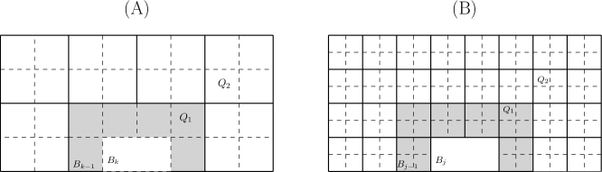
Figure 3. (A) The solid line denotes the partition $\operatorname{\Gamma}_{k-1}^{-1,c};$ the dashed line denotes the refined partition $\operatorname{\Gamma}_{k}^{-1,c}.$ The set difference $B_{k-1}\backslash B_{k}$ (the region in grey) is consists of the new-emerging components $Q_{1}\in\operatorname{\Omega}_{k}.$ Outside $B_{k-1},$ the partition $\operatorname{\Gamma}_{k-1}^{-1,c}$ is refined by the components $Q_{2}\in\Gamma_{k,1}^{-1,c}.$ (B) The solid line denotes the partition $\operatorname{\Gamma}_{j}^{-1,c};$ the dashed line denotes the refined partition $\operatorname{\Gamma}_{k}^{-1,c}.$ The set difference $B_{j-1}\backslash B_{j}$ (the region in grey) is refined by components $Q_{1}\in\operatorname{\Omega}^{\prime}_{k,j}.$ Outside $B_{j-1},$ the partition $\operatorname{\Gamma}_{j}^{-1,c}$ is refined by components $Q_{2}\in\operatorname{\mathcal{W}}_{k,j}.$

Correspondingly, we also split $\Delta_{k}^{(2)}$ into two parts: (i) the refining complexities outside $B_{k-1}$, denoted by $\Delta_{k}^{(2,1)}$; (ii) the new complexities released from $(B_{k-1}\backslash B_{k}),$ denoted by $\Delta_{k}^{(2,2)},$ as follows:

$$\Delta_{k}^{(2)}(\nu) = \sum_{\begin{subarray}{c}Q\in\Gamma^{-1,c}_{k,1},\\ P=fQ\end{subarray}}-\nu(Q)\log\Big{(}\dfrac{\nu(Q)}{\nu(f^{-1}P)}\Big{)}+\sum_{\begin{subarray}{c}Q\in\operatorname{\Omega}_{k},\\ P=fQ\end{subarray}}-\nu(Q)\log\Big{(}\dfrac{\nu(Q)}{\nu(f^{-1}P)}\Big{)}$$ (3.8)

$$=: \Delta_{k}^{(2,1)}(\nu)+\Delta_{k}^{(2,2)}(\nu).$$

The remainder of this subsection estimates $\Delta_{k}^{(2,2)}$ on any $\operatorname{\mathcal{P}}_{\bar{\eta}}(f).$ In the next subsection, we will establish the (non-increasing) monotonicity of $\Delta_{k}^{(2,1)}.$

Lemma 3.5.

For any $\operatorname{\varepsilon}>0$, there exists $k_{2}\in\mathbb{N}$ such that for any $k\geq k_{2}$ and $\nu\in\operatorname{\mathcal{P}}_{\bar{\eta}}(f)$,

$$\sum_{k>k_{2}}\Delta_{k}^{(2,2)}(\nu)<\operatorname{\varepsilon}.$$

Proof.

Since for any $k\geq 1$, $\cup_{Q\in\Omega_{k}}Q=B_{k-1}\setminus B_{k}$,

$$\Delta_{k}^{(2,2)}(\nu) \leq \sum_{Q\in\operatorname{\Omega}_{k}}-\nu(Q)\log\nu(Q).$$ (3.9)

Similar to (3.7), the RHS of (3.9) can be written as

$$\nu(B_{k-1}\setminus B_{k})\sum_{Q\in\Omega_{k}}\phi\Big{(}\frac{\nu(Q)}{\nu(B_{k-1}\setminus B_{k})}\Big{)}-\nu(B_{k-1}\setminus B_{k})\log\nu(B_{k-1}\setminus B_{k})$$

$$=: \Delta_{k}^{(2,2,1)}(\nu)+\Delta_{k}^{(2,2,2)}(\nu).$$

Thus, the estimation of $\Delta_{k}^{(2,2)}$ is reduced to that of $\Delta_{k}^{(2,2,1)}$ and $\Delta_{k}^{(2,2,2)},$ respectively.

We use similar approach in Lemma 3.4 to estimate $\Delta_{k}^{(2,2,1)}.$ First, note that each $Q\in\Omega_{k}$ contains a ball with radius at least $(2^{k+1}L)^{-1}.$ Thus, $\#\Omega_{k}\leq\tilde{C}_{1}^{N(k+1)}L^{N}$ for some constant $\tilde{C}_{1}>0$ independent of $k,L$ and $N$. Then applying Proposition 2.1 with $\{p_{i}\}=\{\frac{\nu(Q)}{\nu(B_{k-1}\setminus B_{k})}\}_{Q\in\operatorname{\Omega}_{k}},$ we have

$$\Delta_{k}^{(2,2,1)}(\nu) \leq \log(\#\tilde{C}_{1}^{N(k+1)}L^{N}),$$ (3.10)

which, using the estimatition as in Lemma 3.2 with $B_{k}$ replaced by $(B_{k}\backslash B_{k-1}),$ yields

$$\Delta_{k}^{(2,2,1)}(\nu) \leq \tilde{C}_{3}\nu(B_{k-1}\setminus B_{k})-\tilde{C}_{4}\int_{B_{k-1}\setminus B_{k}}\log|\operatorname{Jac}(D_{x}f)|d\nu(x)$$

where the constants $\tilde{C}_{3},\tilde{C}_{4}>0$ are independent of $k$ and $\nu.$ Thus, for any $k_{2}\in\operatorname{\mathbb{N}},$

$$\sum_{k>k_{2}}\Delta_{k}^{(2,2,1)}(\nu) \leq \tilde{C}_{3}\nu(B_{k_{2}})-\tilde{C}_{4}\int_{B_{k_{2}}}\log|\operatorname{Jac}(D_{x}f)|d\nu(x).$$ (3.11)

For the estimation of $\Delta_{k}^{(2,2,2)},$ denote

$$I_{1}=\big{\{}k\in\operatorname{\mathbb{N}}:\,\,k\geq-\log\nu(B_{k}\setminus B_{k-1})\big{\}},\quad I_{2}=\big{\{}k\in\operatorname{\mathbb{N}}:\,\,k<-\log\nu(B_{k}\setminus B_{k-1})\big{\}}.$$

Then for any $k_{2}\in\operatorname{\mathbb{N}},$

$$\sum_{k>k_{2}}\Delta_{k}^{(2,2,2)} = \sum_{k\in I_{1},k>k_{2}}-\nu(B_{k}\setminus B_{k-1})\log\nu(B_{k}\setminus B_{k-1})$$

$$+\sum_{k\in I_{2},k>k_{2}}-\nu(B_{k}\setminus B_{k-1})\log\nu(B_{k}\setminus B_{k-1})$$

$$\leq \sum_{k\in I_{1},k>k_{2}}k\nu(B_{k}\setminus B_{k-1})+\sum_{k\in I_{2},k>k_{2}}ie^{-i}.$$

Furthermore, applying Lemma 3.2, we have

$$\sum_{k>k_{2}}\Delta_{k}^{(2,2,2)} \leq C_{3}\nu(B_{k_{2}})-C_{4}\int_{B_{k_{2}}}\log|\operatorname{Jac}(D_{x}f)|d\nu(x)+\sum_{k\in I_{2},k>k_{2}}ke^{-k}.$$ (3.12)

Note that $\sum_{k>k_{2}}ke^{-k}\to 0$ as $k_{2}\to\infty$. Also, as $k_{2}\to\infty,$ both $\int_{B_{k_{2}}}\log|\operatorname{Jac}(D_{x}f)|d\nu(x)$ and $\nu(B_{k_{2}})$ converge to zero uniformly on $\operatorname{\mathcal{P}}_{\bar{\eta}}(f)$. Then combing (3.11) and (3.12), the lemma is proved. ∎

3.2.3. Monotonicity by refining partitions

In this subsection, we demonstrate the (non-increasing) monotonicity for complexities outside any degenerate component $B_{k}\in\operatorname{\Gamma}_{k}^{-1,c}$ during the partition refining process. We remark that distinct from the previous two subsections where the uniform estimations require the measures to admit a uniform degenerate rate, the monotonicity analysis in this subsection applies to all measures in $\operatorname{\mathcal{P}}(M).$

For any $1\leq j\leq k$, define

$$\operatorname{\mathcal{W}}_{k,j} = \Big{\{}Q\in\Gamma^{-1,c}_{k}\backslash\{B_{k}\}:Q\subseteq Q^{\prime}\text{\ for\ some \ }Q^{\prime}\in\Gamma^{-1,c}_{j}\backslash\{B_{j}\}\Big{\}},$$

$$\Omega^{\prime}_{k,j} = \Big{\{}Q\in\Gamma^{-1,c}_{k}\setminus\{B_{k}\}:Q\subseteq Q^{\prime}\,\,\text{for some}\,Q^{\prime}\in\Omega_{j}\Big{\}}.$$

In the same spirit as $\Gamma_{k,1}^{-1,c}$ and $\operatorname{\Omega}_{k}$ in section 3.2.2, both $\operatorname{\mathcal{W}}_{k,j}$ and $\operatorname{\Gamma}_{k,1}^{-1,c}$ are to refine the elements in $\operatorname{\Gamma}_{j}^{-1,c}\backslash\{B_{j}\}$ by using the more refined partition $\operatorname{\Gamma}_{k}^{-1,c}$; see Figure 3(B). In particular, $\operatorname{\mathcal{W}}_{k,k-1}=\Gamma_{k,1}^{-1,c},$ $\operatorname{\Omega}^{\prime}_{k,k}=\operatorname{\Omega}_{k}.$ We denote the respective complexities captured by $\operatorname{\mathcal{W}}_{k,j}$ and $\Omega^{\prime}_{k,j}$ as

$$I_{k,j}(\nu)=\sum_{\begin{subarray}{c}Q\in\operatorname{\mathcal{W}}_{k,j},\\ P=fQ\end{subarray}}-\nu(Q)\log\Big{(}\dfrac{\nu(Q)}{\nu(f^{-1}P)}\Big{)},\quad I^{\prime}_{k,j}(\nu)=\sum_{\begin{subarray}{c}Q\in\operatorname{\Omega}^{\prime}_{k,j},\\ P=fQ\end{subarray}}-\nu(Q)\log\Big{(}\dfrac{\nu(Q)}{\nu(f^{-1}P)}\Big{)}.$$

As a natural linkage to $\Delta_{k}^{(2)}$, it is not hard to see the following.

Proposition 3.6.

Fix any $k_{0}\in\operatorname{\mathbb{N}}.$ Then for any $k>k_{0}$ and $\nu\in\operatorname{\mathcal{P}}(M),$

$$\Delta_{k}^{(2)}(\nu)=I_{k,k_{0}}(\nu)+\sum_{j=k_{0}+1}^{k}I^{\prime}_{k,j}(\nu).$$

In particular, (3.8) is yielded by taking $k_{0}=k-1,$ i.e.,

$$\Delta_{k}^{(2)}(\nu)=I_{k,k-1}(\nu)+I^{\prime}_{k,k}(\nu),$$

where $I_{k,k-1}=\Delta_{k}^{(2,1)},I^{\prime}_{k,k}=\Delta_{k}^{(2,2)}.$

Lemma 3.7.

Given any $\nu\in\operatorname{\mathcal{P}}(M)$ and $j\in\operatorname{\mathbb{N}}.$ Then for any $k\geq j,$ $I_{k,j}(\nu)$ (resp. $I^{\prime}_{k,j}(\nu)$) is non-increasing with respect to $k.$ In particular, $I^{\prime}_{k,j}(\nu)\leq I^{\prime}_{j,j}(\nu)=\Delta_{j}^{(2,2)}(\nu).$

Proof.

We only prove the non-increasing monotonicity for $I_{k,j}.$ The same argument applies to $I^{\prime}_{k,j}$ as well. A key observation is that for any $k^{\prime}>k\geq j,$ the partitions $\operatorname{\Gamma}_{k^{\prime}}^{-1,c}$ and $\operatorname{\Gamma}_{k^{\prime}}$ refine the respective $\operatorname{\Gamma}_{k}^{-1,c}$ and $\operatorname{\Gamma}_{k}$ in a consistent manner. More specifically, for any $Q\in\operatorname{\mathcal{W}}_{k,j},$ since $f|_{Q}$ is a diffeomorphism, then there is a one-one correspondence, through $f,$ between the refining of $P$ by $\operatorname{\Gamma}_{k^{\prime}}$ and the refining of $Q$ by $\operatorname{\mathcal{W}}_{k^{\prime},j}$; see Figure 4.

Figure 4. The component $Q\in\operatorname{\mathcal{W}}_{k,j}$ (resp. $P\in\operatorname{\Gamma}_{k}$) is refined by components $Q^{\prime}\in\operatorname{\mathcal{W}}_{k^{\prime},j}$ (resp. $P^{\prime}\in\operatorname{\Gamma}_{k^{\prime}}$) in a one-one corresponding way such that each $P^{\prime}=fQ^{\prime}.$

Thus, $I_{k^{\prime},j}$ can be written as

$$I_{k^{\prime},j} = \sum_{Q\in\operatorname{\mathcal{W}}_{k,j}}\sum_{\begin{subarray}{c}Q^{\prime}\in\operatorname{\mathcal{W}}_{k^{\prime},j},\\ Q^{\prime}\subseteq Q,P^{\prime}=fQ^{\prime}\end{subarray}}\nu(f^{-1}P^{\prime})\phi\Big{(}\dfrac{\nu(Q^{\prime})}{\nu(f^{-1}P^{\prime})}\Big{)}$$ (3.13)

$$= \sum_{\begin{subarray}{c}Q\in\operatorname{\mathcal{W}}_{k,j},\\ P=fQ\end{subarray}}\nu(f^{-1}P)\sum_{\begin{subarray}{c}Q^{\prime}\in\operatorname{\mathcal{W}}_{k^{\prime},j},\\ Q^{\prime}\subseteq Q,P^{\prime}=fQ^{\prime}\end{subarray}}\dfrac{\nu(f^{-1}P^{\prime})}{\nu(f^{-1}P)}\phi\Big{(}\dfrac{\nu(Q^{\prime})}{\nu(f^{-1}P^{\prime})}\Big{)}.$$

Since $\{P^{\prime}\}$ is a refinement of $P$, applying Proposition 2.1 with $\{p_{i}\}=\{\frac{\nu(f^{-1}P^{\prime})}{\nu(f^{-1}P)}\}_{P^{\prime}},$ $\{x_{i}\}=\{\frac{\nu(Q^{\prime})}{\nu(f^{-1}P^{\prime})}\}_{Q^{\prime}},$ for the first summation in (3.13), we have

$$\sum_{\begin{subarray}{c}Q^{\prime}\in\operatorname{\mathcal{W}}_{k^{\prime},j},\\ Q^{\prime}\subseteq Q,P^{\prime}=fQ^{\prime}\end{subarray}}\dfrac{\nu(f^{-1}P^{\prime})}{\nu(f^{-1}P)}\phi\Big{(}\dfrac{\nu(Q^{\prime})}{\nu(f^{-1}P^{\prime})}\Big{)}\leq\phi\Big{(}\sum_{\begin{subarray}{c}Q^{\prime}\in\operatorname{\mathcal{W}}_{k^{\prime},j},\\ Q^{\prime}\subseteq Q,\end{subarray}}\dfrac{\nu(Q^{\prime})}{\nu(f^{-1}P)}\Big{)}=\phi\Big{(}\dfrac{\nu(Q)}{\nu(f^{-1}P)}\Big{)}.$$

Therefore,

$$I_{k^{\prime},j}\leq\sum_{\begin{subarray}{c}Q\in\operatorname{\mathcal{W}}_{k,j},\\ P=fQ\end{subarray}}\nu(f^{-1}P)\phi\Big{(}\dfrac{\nu(Q)}{\nu(f^{-1}P)}\Big{)}=\sum_{\begin{subarray}{c}Q\in\operatorname{\mathcal{W}}_{k,j},\\ P=fQ\end{subarray}}-\nu(f^{-1}P)\log\Big{(}\dfrac{\nu(Q)}{\nu(f^{-1}P)}\Big{)}=I_{k,j}.$$

∎

Fixing any $k_{0}\in\operatorname{\mathbb{N}},$ by Lemma 3.7, it is well-defined to put

$$I_{k_{0}}(\nu)=\lim\limits_{k\rightarrow\infty}I_{k,k_{0}}(\nu)=\inf\limits_{k\geq k_{0}}I_{k,k_{0}}(\nu).$$

For each $k\geq k_{0},$ since $\operatorname{\mathcal{W}}_{k,k_{0}}$ only contains the components of $\operatorname{\Gamma}_{k}^{-1,c}$ not intersecting with the degenerate component $B_{k_{0}}\in\operatorname{\Gamma}_{k_{0}}^{-1,c}$. Then as $k$ increases, $I_{k,k_{0}}$ approximates only the part of complexities in folding entropy away from $\Sigma_{f}$. Therefore,

$$I_{k_{0}}(\nu)\leq F_{f}(\nu),\quad\forall\nu\in\operatorname{\mathcal{P}}(M).$$ (3.14)

Also, as each $I_{k,k_{0}}$ is a finite summation, we directly obtain the upper semi-continuity property of $I_{k_{0}}$ on $\operatorname{\mathcal{P}}(M).$

Proposition 3.8.

For each $k\geq 1,$ $I_{k}(\cdot)$ is upper semi-continuous on $\operatorname{\mathcal{P}}(M).$

Proof.

Given any $\mu\in\operatorname{\mathcal{P}}(M).$ By a translation if necessary, we may assume $\mu(\partial\Gamma_{k})=\mu(\partial\operatorname{\Gamma}_{k}^{-1,c})=0$ for all $k\in\operatorname{\mathbb{N}}.$ Thus, for any $k\geq k_{0},$

$$I_{k,k_{0}}(\nu)=\sum_{\begin{subarray}{c}Q\in\operatorname{\mathcal{W}}_{k,k_{0}},\\ P=fQ\end{subarray}}-\nu(Q)\log\Big{(}\dfrac{\nu(Q)}{\nu(f^{-1}P)}\Big{)}$$

is continuous at $\mu.$ This implies the upper semi-continuity of $I_{k}=\inf_{k\geq k_{0}}I_{k,k_{0}}$ on $\operatorname{\mathcal{P}}(M).$ ∎

Now we are at the position to prove Theorem 1.1.

Proof of Theorem 1.1. Given any $\operatorname{\varepsilon}>0,$ by Lemmas 3.4 and 3.5, for $k_{0}=\min\{k_{1},k_{2}\}$ we have

$$\Delta_{k}^{(1)}(\nu)<\operatorname{\varepsilon},\quad\sum_{k_{0}\leq j\leq k}\Delta_{j}^{(2,2)}(\nu)<\operatorname{\varepsilon},\quad\forall k\geq k_{0}.$$

By Proposition 3.6 and Lemma 3.7,

$$\Delta_{k}^{(2)}(\nu)\leq I_{k,k_{0}}(\nu)+\sum_{k_{0}<j\leq k}\Delta_{j}^{(2,2)}(\nu)<I_{k,k_{0}}(\nu)+\operatorname{\varepsilon}.$$

It then follows from (3.6) that

$$F_{f}(\nu)<I_{k,k_{0}}(\nu)+2\operatorname{\varepsilon},\quad\forall k\geq k_{0},$$ (3.15)

where we enlarge $k_{0}$ if necessary.

Now, let $\{\mu_{i}\}\subseteq\mathcal{M}_{\bar{\eta}}(f)$ such that $\mu_{i}$ converge to $\mu$. Applying (3.15) with $\nu$ being $\{\mu_{i}\}$, together with Proposition 3.8, we have

$$\limsup_{i\to\infty}F_{f}(\mu_{i})\leq\limsup_{i\to\infty}I_{k,k_{0}}(\mu_{i})+2\operatorname{\varepsilon}\leq I_{k,k_{0}}(\mu)+2\operatorname{\varepsilon},\quad\forall k\geq k_{0},$$

which, by (3.14), implies

$$\limsup\limits_{i\to\infty}F_{f}(\mu_{i})\leq F_{f}(\mu)+2\operatorname{\varepsilon}.$$

The proof of Theorem 1.1 is concluded by the arbitrariness of $\operatorname{\varepsilon}$. $\Box$

4. Applications to interval maps

In this section, we focus on the one-dimensional setting by considering $C^{r}(r>1)$ interval maps. As applications of Theorem 1.1, we will show the upper semi-continuity of both the metric entropy $h_{\mu}(f)$ and the dimension $\operatorname{dim}(\mu)$ when measures with uniform degenerate rate are considered. To achieve this, we will establish a entropy formula and a dimension formula to the very general nature of $f.$

4.1. Upper semi-continuity of metric entropy

For a $C^{r}(r>1)$ interval map $f$ and $\mu\in\operatorname{\mathcal{M}}_{inv}(f),$ recall the following inequalities for the metric entropy $h_{\mu}(f)$:

$$h_{\mu}(f) \leq \displaystyle\int\max\{\lambda(f,x),0\}d\mu(x),$$ (4.1)

$$h_{\mu}(f) \leq F_{f}(\mu)-\displaystyle\int\min\{\lambda(f,x),0\}d\mu(x),$$ (4.2)

where $\lambda(f,x)$ is the Lyapunov exponent of $f$ at $x$. The first inequality in (4.1) is the well-known Margulis-Ruelle inequality [34], and (4.2) is the folding-type Ruelle inequality (1.2) applied in the one-dimensional setting. The following theorem shows that in the one-dimensional setting, the metric entropy and folding entropy are actually equal.

Theorem 4.1.

Let $f$ be a $C^{r}(r>1)$ map on an interval $I$. Then for any $\mu\in\mathcal{M}_{inv}(f)$, it holds that

$$h_{\mu}(f)=F_{f}(\mu).$$ (4.3)

Proof.

First, we have that

$$h_{\mu}(f)\geq F_{\mu}(f),\quad\forall\mu\in\operatorname{\mathcal{M}}_{inv}(f).$$ (4.4)

To see this, let $\{\xi_{n}\}_{n\geq 1}$ be a sequence of increasing finite partitions of $I$ such that $\bigvee\limits_{n\geq 1}\xi_{n}=\epsilon(\mod\mu)$. Then by (2.1), for each $n\geq 1,$

$$h_{\mu}(f,\xi_{n})=H_{\mu}(\xi_{n}|\bigvee\limits_{i=1}^{\infty}f^{-i}\xi_{n})\geq H_{\mu}(\xi_{n}|f^{-1}\epsilon),$$

where the inequality is by observing that $f^{-1}\epsilon\succeq\bigvee\limits_{i=1}^{\infty}f^{-i}\xi_{n}=f^{-1}(\bigvee\limits_{i=0}^{\infty}f^{-i}\xi_{n}).$ Thus,

$$h_{\mu}(f)=\lim\limits_{n\rightarrow\infty}h_{\mu}(f,\xi_{n})\geq\lim\limits_{n\rightarrow\infty}H_{\mu}(\xi_{n}|f^{-1}\epsilon)=H_{\mu}(\epsilon|f^{-1}\epsilon).$$

Now, we only need to show $h_{\mu}(f)\leq F_{f}(\mu).$ Denote

$$A_{1}=\{x\in I:\lambda(f,x)\leq 0\}\quad\text{and}\quad A_{2}=\{x\in I:\lambda(f,x)>0\}.$$

Without loss of generality, assume that $A_{1}$ and $A_{2}$ are both positive $\mu$-measured, since for otherwise, the situations would be easier. Let $\mu^{(i)}=\mu/\mu(A_{i}),i=1,2$, and we write $\mu=\sum_{i=1,2}\mu(A_{i})\mu^{(i)}.$

By (4.1) we have $h_{\mu^{(1)}}(f)=0.$ Then combined with (4.4), one gets

$$F_{f}(\mu)=h_{\mu^{(1)}}(f)=0.$$ (4.5)

For $\mu^{(2)},$ one directly gets, from (4.2), that

$$h_{\mu^{(2)}}(f)\leq F_{f}(\mu^{(2)}).$$ (4.6)

Since both $A_{1}$ and $A_{2}$ are $f$-invariant (mod $\mu$), we have

$$F_{f}(\mu)=\int_{I}H_{\tilde{\mu}_{x}}(\epsilon)d\mu=\sum_{i=1,2}\int_{A_{i}}H_{\tilde{\mu}_{x}}(\epsilon)d\mu=\sum_{i=1,2}\mu(A_{i})F_{f}(\mu^{(i)}),$$

where recall that $\tilde{\mu}_{x}$ is the disintegration of $\mu$ along the partition $\{f^{-1}x\}.$ Now, combining (4.5) and (4.6), we have

$$h_{\mu}(f)=\sum_{i=1,2}\mu^{(i)}(A_{i})h_{\mu^{(i)}}(f)\leq\sum_{i=1,2}\mu^{(i)}(A_{i})F_{f}({\mu^{(i)}})=F_{f}(\mu).$$

∎

Proof of Theorem 1.3. By (4.3), Theorem 1.3 is a direct consequence of Theorem 1.1.

4.2. Upper semi-continuity of dimension

For an ergodic $\mu\in\operatorname{\mathcal{M}}_{inv}(f),$ the Lyapunov exponents of $f$ are constants with respect to $\mu$-a.e. $x$, and in the one-dimensional setting particularly, we have only one Lyapunov exponent and denote it as $\lambda(\mu)$. The main estimation of this subsection is to establish the following dimension formula which relates the dimension to metric entropy through Lyapunov exponent for all $C^{r}(r>1)$ interval maps.

Theorem 4.2.

Let $f$ be a $C^{r}(r>1)$ map on an interval $I.$ Given a hyperbolic $\mu\in\operatorname{\mathcal{M}}_{erg}(f)$, then $\mu$ is exact dimensional and satisfies

$$h_{\mu}(f)=\lambda^{+}(\mu)\operatorname{dim}(\mu),$$ (4.7)

where $\lambda^{+}(\mu)=\max\{\lambda(\mu),0\}.$

Before proceeding to its proof, we would like to state two remarks of Theorem 4.2: (i) The hyperbolicity assumption of $\mu$ is sharp. Both $C^{r}(r<\infty)$ and analytical examples are constructed in respective [20] and [17] showing that for a non-hyperbolic ergodic measure $\mu$ with zero exponent, the local dimension may not exist almost everywhere; (ii) The formula (4.7) is proved by Ledrappier in [19] for an interval map $f$ under the assumption that the entropy of the partition by the degenerate sets of $f$ and $f^{\prime}$ are finite. Thus, Theorem 4.2 is a general result in this respect.

A key step in the proof of Theorem 4.2 is an integrable version of the classical Brin-Katok formula; see Lemma 4.5. Let $f$ be a continuous map on a compact metric space $M$. For any $\delta>0$, $n\in\mathbb{N}$ and $x\in M$, define

$$B_{n}(x,\delta)=\big{\{}y\in M:d(f^{i}x,f^{i}y)<\delta,0\leq i\leq n-1\big{\}}.$$

The following local entropy formula was established by Brin and Katok in [4].

Proposition 4.3 (Brin-Katok [4]).

Let $\mu\in\operatorname{\mathcal{M}}_{inv}(f).$ Then for $\mu$-a.e. $x\in M$,

$$\lim_{\delta\to 0}\liminf_{n\to\infty}-\frac{\log\mu(B_{n}(x,\delta))}{n}=\lim_{\delta\to 0}\limsup_{n\to\infty}-\frac{\log\mu(B_{n}(x,\delta))}{n}:=h_{\mu}(f,x),$$ (4.8)

where the local entropy $h_{\mu}(f,x)$ satisfies

$$\int_{X}h_{\mu}(f,x)d\mu=h_{\mu}(f).$$

In particular, if $\mu$ is ergodic, then

$$h_{\mu}(f,x)=h_{\mu}(f),\quad\mu{\text{-a.e.}}\ x\in M.$$

We will prove an integrable version of (4.8) by replacing $\delta$ with any $\log$-integrable function. To be specific, let $\mathscr{S}$ be the set of all functions $\psi:M\to\mathbb{R}^{+}$ satisfying

$$\int-\log\psi(x)d\mu(x)<\infty.$$

For any $\psi\in\mathscr{S}$, $n\in\mathbb{N}$, and $x\in M$ define

$$B_{n}(x,\psi)=\big{\{}y\in M:d(f^{i}x,f^{i}y)<\psi(f^{i}x),0\leq i\leq n-1\big{\}}.$$

It has been shown by Mañé that

Proposition 4.4 (Mañé[25]).

For any $\psi\in\mathscr{S}$,

$$\int\limsup_{n\to\infty}-\frac{\log\mu(B_{n}(x,\psi))}{n}d\mu(x)\leq h_{\mu}(f).$$

Based on Propositions 4.3 and 4.4, we obtain the following generalized local entropy formula.

Lemma 4.5.

Let $f$ be a continuous map on a compact metric space $M$ and $\mu\in\operatorname{\mathcal{M}}_{inv}(f).$ Then given any $\psi\in\mathscr{S},$ for $\mu$-a.e. $x\in M$,

$$\lim_{\delta\to 0}\liminf_{n\to\infty}\ -\frac{\log\mu(B_{n}(x,\psi^{\delta}))}{n}=\lim_{\delta\to 0}\limsup_{n\to\infty}-\frac{\log\mu(B_{n}(x,\psi^{\delta}))}{n}=h_{\mu}(f,x),$$

where $\psi^{\delta}(x):=\min\{\psi(x),\delta\}$ and $h_{\mu}(f,x)$ is given as in Proposition 4.3.

Proof.

For one thing, since $B_{n}(x,\psi^{\delta})\subseteq B_{n}(x,\delta)$, we have

$$\lim_{\delta\to 0}\liminf_{n\to\infty}-\frac{\log\mu(B_{n}(x,\psi^{\delta}))}{n} \geq h_{\mu}(f,x)$$ (4.9)

which, by (4.8), yields

$$\int_{M}\lim_{\delta\to 0}\liminf_{n\to\infty}-\frac{\log\mu(B_{n}(x,\psi^{\delta}))}{n}d\mu \geq \int_{M}h_{\mu}(f,x)d\mu=h_{\mu}(f).$$ (4.10)

For another, by Proposition 4.4,

$$\int_{M}\lim_{\delta\to 0}\limsup_{n\to\infty}-\frac{\log\mu(B_{n}(x,\psi^{\delta}))}{n}d\mu=\lim_{\delta\to 0}\int_{M}\limsup_{n\to\infty}-\frac{\log\mu(B_{n}(x,\psi^{\delta}))}{n}d\mu\leq h_{\mu}(f).$$ (4.11)

Combining (4.10) and (4.11), we have

$$\int_{M}\lim_{\delta\to 0}\limsup_{n\to\infty}-\frac{\log\mu(B_{n}(x,\psi^{\delta}))}{n}d\mu = \int_{X}\lim_{\delta\to 0}\liminf_{n\to\infty}-\frac{\log\mu(B_{n}(x,\psi^{\delta}))}{n}d\mu$$

$$= \int_{X}h_{\mu}(f,x)d\mu=h_{\mu}(f).$$

Then together with (4.9), for $\mu$-a.e. $x\in M,$ it holds that

$$\lim_{\delta\to 0}\limsup_{n\to\infty}\ -\frac{\log\mu(B_{n}(x,\psi^{\delta}))}{n}=\lim_{\delta\to 0}\liminf_{n\to\infty}-\frac{\log\mu(B_{n}(x,\psi^{\delta}))}{n}=h_{\mu}(f,x).$$

∎

Proof of Theorem 4.2: Denote $\alpha=\min\{r-1,1\}$ and $L=\max_{x\in I}\{|f^{\prime}(x)|,1\}$. Then $f$ is $C^{1+\alpha},$ i.e., for some constant $K>0,$ $|f^{\prime}(x)-f^{\prime}(y)|\leq K|x-y|^{\alpha},\ \forall x,y\in I.$ Take small $\gamma\in(0,1),$ and for any $x\in I\backslash\Sigma_{f}$ let $\rho(x)=(\frac{\gamma|f^{\prime}(x)|}{K})^{\frac{1}{\alpha}}.$ Then

$$(1-\gamma)|f^{\prime}(x)|\leq|f^{\prime}(y)|\leq(1+\gamma)|f^{\prime}(x)|,\quad\forall\,y\in B(x,\rho(x)),$$

which implies that $f|_{B(x,\rho(x))}$ is a local diffeomorphism.

By the definition of Lyapunov exponent, for $\mu$-a.e. $x\in I$,

$$\int_{M}\log|f^{\prime}(x)|d\mu(x)=\lim_{n\to\infty}\frac{1}{n}\sum_{i=0}^{n-1}\log|f^{\prime}(f^{i}x)|=\lambda(\mu),$$

or equivalently,

$$\lim_{n\to\infty}\frac{1}{n}\sum_{i=0}^{n-1}\log\big{|}(f^{-1}\mid_{f(B(f^{i}x,\rho(f^{i}x)))})^{\prime}(f^{i+1}x)\big{|}=-\lambda(\mu).$$

Thus, there exists $N(x)\in\mathbb{N}$ such that for any $n\geq N(x),$

$$\prod_{i=0}^{n-1}|f^{\prime}(f^{i}x)|\in\big{(}e^{n(\lambda(\mu)-\gamma)},\,e^{n(\lambda(\mu)+\gamma)}\big{)},$$ (4.12)

or equivalently

$$\prod_{i=0}^{n-1}\big{|}(f^{-1}\mid_{f(B(f^{i}x,\rho(f^{i}x)))})^{\prime}(f^{i+1}x)\big{|}\in\big{(}e^{n(-\lambda(\mu)-\gamma\big{)}},\,e^{n(-\lambda(\mu)+\gamma)}).$$ (4.13)

Let $D(x)=\min_{0\leq i\leq N(x)}\{\rho(f^{i}x),1\}$. Note that the integrability of $\log|f^{\prime}(x)|$ (and thus $\log\rho(x)$) implies $\mu(\Sigma_{f})=0,$ which in turns yields $D(x)>0$ for $\mu$-a.e. $x\in I.$

Now, for any small $\delta\in(0,1)$, denote $A_{\delta}=\{x\in I:\rho(x)\leq\delta\},$ and for any $n\in\mathbb{N}$, define

$$\Phi_{n}(x)=\prod_{0\leq i<n:f^{i}x\in A_{\delta}}\,\,\rho(f^{i}x).$$

Then $\delta\Phi_{n}(x)\leq\rho^{\delta}(f^{i}x),0\leq i<n.$ By the Birkhoff ergodic theorem, for $\mu$-a.e. $x\in I,$

$$\frac{\log\Phi_{n}(x)}{n}\to\int_{A_{\delta}}\log\rho(z)d\mu(z),\quad n\to\infty.$$ (4.14)

Now, for any $n\in\operatorname{\mathbb{N}}$ let

$$\tilde{r}_{n} = D(x)L^{-N(x)}\delta\Phi_{n}(x)(1+\gamma)^{-n}e^{-n(\lambda(\mu)+\gamma)},$$

$$\hat{r}_{n} = (1-\gamma)^{-n}e^{-n(\lambda(\mu)-\gamma)}.$$

Obviously, $\tilde{r}_{n}\to 0,\hat{r}_{n}\to 0$ as $n\to\infty.$

Claim 4.6.

For $\mu$-a.e. $x\in M$ and $n\geq N(x),$

$$B(x,\tilde{r}_{n})\subset B_{n}(x,\rho^{\delta})\subset B(x,\hat{r}_{n}).$$ (4.15)

We postpone the proof of Claim 4.6 for the time being and proceed to finish the proof of Theorem 4.2. By (4.15) we have

$$\overline{\operatorname{dim}}(x)=\limsup_{n\to\infty}\frac{\log\mu(B(x,\hat{r}_{n}))}{\log\hat{r}_{n}}\leq\limsup_{n\to\infty}\frac{\log\mu(B_{n}(x,\rho^{\delta}))}{-n}\frac{1}{\log(1-\gamma)+\lambda(\mu)-\gamma}.$$

Then Lemma 4.5, together with the arbitrariness of $\delta$ and $\gamma$, yields

$$\overline{\operatorname{dim}}(x)\leq\frac{h_{\mu}(f,x)}{\lambda(\mu)}.$$

Since $\mu$ is ergodic, it follows from Propositions 2.2 and 4.3 that

$$\overline{\operatorname{dim}}(\mu)\leq\dfrac{h_{\mu}(f)}{\lambda(\mu)}.$$ (4.16)

On the other hand, (4.15) also yields

$$\underline{\operatorname{dim}}(x) = \liminf_{n\to\infty}\frac{\log\mu(B(x,\tilde{r}_{n}))}{\tilde{r}_{n}}$$

$$\geq \liminf_{n\to\infty}\frac{\log\mu(B_{n}(x,\rho^{\delta}))}{-n}\frac{1}{\frac{\log\Phi_{n}(x)}{n}+\log(1+\gamma)+\lambda(\mu)+\gamma}$$

$$= \liminf_{n\to\infty}\frac{\log\mu(B_{n}(x,\rho^{\delta}))}{-n}\cdot\frac{1}{\int_{A_{\delta}}\log\rho(z)d\mu(z)+\lambda(\mu)+\gamma},$$

where the last equality is from (4.14). Note that $\mu(A_{\delta})\to 0$ as $\delta\to 0.$ Thus, $\int_{A_{\delta}}\log\rho(z)d\mu(z)$ can be arbitrarily small by choosing small $\delta\in(0,1)$. Again, applying Lemma 4.5, Propositions 2.2 and 4.3, together with the arbitrariness of $\delta$ and $\gamma$, we have

$$\underline{\operatorname{dim}}(\mu)\geq\frac{h_{\mu}(f)}{\lambda(\mu)}.$$ (4.17)

Combining (4.17) and (4.16), the proof of Theorem 4.2 is concluded.

Proof of Claim 4.6: To prove $\tilde{B}_{n}(x)\subset B_{n}(x,\rho^{\delta}),$ we only need to show

$$f^{i}(\tilde{B}_{n}(x))\subset B(f^{i}x,\rho^{\delta}(f^{i}x)),\quad 0\leq i<n.$$ (4.18)

First, it is not hard to see that (4.18) holds for $0\leq i\leq N(x).$ Now, assume that for $N(x)<i\leq n,$ (4.18) holds for $j=0,1,\cdots,i-1.$ Then for any $y\in\tilde{B}_{n}(x),$ by (4.12) we have

$$\prod_{j=0}^{i-1}\big{|}f^{\prime}(f^{j}y)\big{|}\leq\Big{(}\prod_{j=0}^{i-1}\big{|}f^{\prime}(f^{j}x)\big{|}\Big{)}(1+\gamma)^{i}\leq e^{i(\lambda(\mu)+\gamma)}(1+\gamma)^{i}\leq e^{n(\lambda(\mu)+\gamma)}(1+\gamma)^{n}.$$

Thus,

$$f^{i}(\tilde{B}_{n}(x))\subset B(f^{i}x,D(x)L^{-N(x)}\delta\Phi_{n}(x))\subset B(f^{i}x,\delta\Phi_{n}(x))\subset B(f^{i}x,\rho^{\delta}(f^{i}x)).$$

Then the induction establishes (4.18).

To establish $B_{n}(x,\rho^{\delta})\subset\hat{B}_{n}(x),$ note that for any $y\in f^{n}(B_{n}(x,\rho^{\delta})),$

$$f^{i}y\in B(f^{i}x,\rho(f^{i}x)),\ 0\leq i\leq n,$$

and hence for $0\leq i\leq n$,

$$\big{|}f^{-1}\mid_{f(B(f^{i}(x),\rho(f^{i}x))})^{\prime}(f^{i+1}y)\big{|}\leq(1-\gamma)^{-1}\big{|}f^{-1}\mid_{f(B(f^{i}(x),\rho(f^{i}x))})^{\prime}(f^{i+1}x)\big{|}.$$

Then (4.13) yields

$$\prod_{0\leq i<n}|(f^{-1}\mid_{f(B(f^{i}(x),\rho(f^{i}x))})^{\prime}(f^{i+1}y)|\leq(1-\gamma)^{-n}e^{-n(\lambda(\mu)-\gamma)}.$$

By noting that $f^{n}|_{B_{n}(x,\rho^{\delta})}$ is a local diffeomorphism, we have

$$B_{n}(x,\rho^{\delta})\subset\hat{B}_{n}(x).$$

This completes the proof of Claim 4.6. $\Box$

Proof of Theorem 1.4.

First, note that the Lyapunov exponent $\lambda(\nu)=\int\log|f^{\prime}(x)|d\nu(x)$ is continuous on $\operatorname{\mathcal{M}}_{\bar{\eta},erg}(f)$. Thus, suppose that $\{\mu_{i}\}\subseteq\mathcal{M}_{\bar{\eta},erg}(f)$ and $\mu_{i}$ converge to some hyperbolic $\mu\in\mathcal{M}_{\bar{\eta},erg}(f)$. We have that $\{\mu_{i}\}$ are hyperbolic for all $i$ large such that $\lambda(\mu_{i})>0$ (resp. $<0$) if $\lambda(\mu)>0$ (resp. $<0$). Assume $\lambda(\mu)<0.$ In this case, every one of $\mu$ and $\mu_{i}$ ($i\gg 1$) is supported at some contracting periodic orbit, and hence the corresponding $\operatorname{dim}(\mu)$ and $\operatorname{dim}(\mu_{i})$ are always zero, and Theorem 1.4 is proved. Now, assume $\lambda(\mu)>0,$ and hence $\lambda(\mu_{i})>0,i\gg 1.$ By Theorem 4.2, the dimension formula (4.7) applies for all $\mu,\mu_{i}(i\gg 1).$ Since the continuity of metric entropy (by Theorem 1.3) and the Lyapunov exponent holds on $\operatorname{\mathcal{M}}_{\bar{\eta},erg}(f),$ we have $\limsup_{i\to\infty}\operatorname{dim}(\mu_{i})\leq\operatorname{dim}(\mu).$ Thus, the upper semi-continuity of $\operatorname{dim}(\cdot)$ on $\operatorname{\mathcal{M}}_{\bar{\eta},erg}(f)$ is obtained. ∎

5. An example of interval maps

In this section, for each $r\in(1,\infty),$ we construct a $C^{r}$ interval map $f$ which admits ergodic measures with positive entropy as non upper semi-continuity points of the metric (or folding entropy). Before describing the example, we recall a quantitative proposition about the (one-sided) shift that will be used in our discussion.

Proposition 5.1 (see Theorem 4.26 and its Remark in [39]).

Consider the $k$-full shift $(\Sigma_{k},\sigma)$. For any probability vector $(p_{0},\cdots,p_{k-1}),$ the Markov measure associated with the $(p_{0},\cdots,p_{k-1})$-shift is ergodic with the entropy equals $\sum\limits_{i=0}^{k-1}-p_{i}\log p_{i}.$ In particular, the metric entropy of $(\frac{1}{k},\cdots,\frac{1}{k})$-shift achieves the topological entropy of the full shift $(\Sigma_{k},\sigma)$ which equals to $\log k.$

By Proposition 5.1, given any full shift with topological entropy $h,$ any real number in $(0,h]$ can be achieved by an ergodic invariant measure with full support.

Figure 5. Accumulation of small horseshoes

5.1. Example description

In this subsection, we describe in detail how the interval map $f:I\rightarrow I$ is constructed on $I=[0,1]$; see Figure 5 for its qualitative depiction. In Figure 5, $I_{1}$ and $I_{2}$ are two subintervals of $I$ on which $f$ acts linearly with slope $\lambda$ such that

$$f(I_{i})\supseteq I_{1}\cup I_{2},\quad i=1,2.$$

Let

$$\Lambda=\bigcap\limits_{i=0}^{\infty}f^{-i}(I_{1}\cup I_{2}).$$

Then $(f,\Lambda)$ is uniformly expanding and conjugate to a (one-sided) full shift of two symbols. Thus, the topological entropy $h_{\operatorname{top}}(f|_{\Lambda})=\log 2$.

In the following, for any subinterval $J\subset I$, by $|J|$ we mean the length of $J$. Any $y\in I$ stands for either a point in $I$ or a real number when $I$ is considered as a subinterval of $\mathbb{R}$. Let $x_{*}$ and $x_{*}^{\prime}$ be the left and right end point of $I_{1}$ and $I_{2}$, respectively. We further require that $x_{*}$ is a fixed point of $f$ such that $f(x_{*}^{\prime})=f(x_{*})=x_{*}$. For simplicity, set $a=x_{*}=|I_{1}|=|I_{2}|$ and $d_{H}(I_{1},I_{2})=3a$. Also, let $\lambda$ be large enough so that

$$I_{1}\cup I_{2}\subset[x_{*},x_{*}+\dfrac{a\lambda}{2}].$$

Since $(f,\Lambda)$ conjugates to a one-sided 2-full shift, by Proposition 5.1, for any $c\in(0,c_{0})$ where $c_{0}=\min\{\log 2,\frac{1}{r}\log\lambda\},$ we can find $\mu\in\operatorname{\mathcal{M}}_{erg}(f)$ supported on $\Lambda$ such that

$$h_{\mu}(f)=c<\frac{1}{r}\log\lambda.$$ (5.1)

Take $\delta_{0}=a/(2\lambda).$ Observing that $x_{*}\in\Lambda$, we can choose a generic point $x_{0}\in\operatorname{supp}\mu\cap[x_{*},\delta_{0}/2]$ of $\mu$ in the sense that

$$\dfrac{1}{n}\sum\limits_{i=0}^{n-1}\delta_{f^{i}(x_{0})}\rightarrow\mu,\quad\text{as}\,\,n\rightarrow\infty,$$

in the weak*-topology. As denoted in Figure 5, arrange $z_{0}$ to be a preimage of $x_{0}$ lying on the right side of $x_{*}^{\prime}$ such that $|x_{*}^{\prime}-z_{0}|=a.$ Also, we can require that $f$ remains linear with slope $\lambda$ in the $\delta_{0}$-neighborhood of $I_{1}\cup I_{2}$ since $d_{H}(I_{1},I_{2})=3a$.

Lemma 5.2.

Let $\delta_{1}=x_{0}-x_{*}$. Then there exist $N_{1},N_{2}\in\mathbb{N}$ such that

$$f^{N_{1}}([x_{0}-\delta_{1},x_{0}])\supset[z_{0}-a,z_{0}+3a],\quad f^{N_{2}}([x_{0},x_{0}+\delta_{1}])\supset[z_{0}-a,z_{0}+3a].$$

Proof.

Since $x_{*}$ is a fixed point, the expanding property of $f$ on $I_{1}$ gives certain $N_{1}\in\mathbb{N}$ such that

$$f^{N_{1}}([x_{0}-\delta_{1},x_{0}])\supset f(I_{1})\supset[z_{0}-a,z_{0}+3a].$$

Then by the continuity of $f,$ there exists $\delta\in(0,\delta_{1})$ such that

$$f^{N_{1}}([x_{0}-\delta_{1}+\delta,x_{0}])\supset[z_{0}-a,z_{0}+3a].$$

Recall that $x_{0}$ is a generic point of $\mu$. Since $\mu([x_{0}-\delta_{1},x_{0}-\delta_{1}+\delta])>0$, there exists $t\in\mathbb{N}$ such that

$$f^{t}(x_{0})\in[x_{0}-\delta_{1},x_{0}-\delta_{1}+\delta].$$

Now, consider the $f$-iterates of $[x_{0},x_{0}+\delta_{1}]$ successively cut by the interval $[x_{*}-\delta_{0},x_{*}^{\prime}+\delta_{0}]$. Then there exists $t_{0}>0$ such that for each $i>t_{0},$ $f^{i}([x_{0},x_{0}+\delta_{1}])$ contains an interval $R_{i}$ of length $\delta_{0}$ with $f^{i}(x_{0})$ being one of its end points. In particular, let $t>t_{0}.$ Now, we proceed according to the cases where $f^{t}(x_{0})$ is the left and right end point of $R_{t},$ respectively. If $f^{t}(x_{0})$ is the left end point, we have $R_{t}\supset[x_{0}-\delta_{1}+\delta,x_{0}],$ and hence

$$f^{t+N_{1}}([x_{0},x_{0}+\delta_{1}])\supset f^{N_{1}}(R_{t})\supset[z_{0}-a,z_{0}+3a].$$

Then $N_{2}=t+N_{1}$ is as desired; If $f^{t}(x_{0})$ is the right end point of $R_{t}$, then

$$R_{t}\supset[x_{0}-\delta_{1},f^{t}x_{0}].$$

Once more, using the expanding property of $f$ on $I_{1}$, there exists $t^{\prime}\in\mathbb{N}$, such that

$$f^{t^{\prime}}([x_{0}-\delta_{1},f^{t}x_{0}])\supset[z_{0}-a,z_{0}+3a].$$

In this case, let $N_{2}=t+t^{\prime}$. So the proof is finished. ∎

By Lemma 5.2 and the continuity of $f$, there exists $\eta>0$ such that for any $x\in[x_{0}-\eta,x_{0}+\eta]$,

$$f^{N_{1}}([x-\delta_{1},x])\supset[z_{0},z_{0}+2a],\quad f^{N_{2}}([x,x+\delta_{1}])\supset[z_{0},z_{0}+2a].$$ (5.2)

Since $x_{0}$ is a generic point and $\mu([x_{0}-\eta,x_{0}+\eta])>0$, there exist $n_{1}<n_{2}<\cdots<n_{k}<\cdots$ such that $f^{n_{k}}(x_{0})\in[x_{0}-\eta,x_{0}+\eta]$. Now, let $\{J_{n}\}_{n\geq 1}$ be a sequence of disjoint subintervals of $I$ accumulating to $z_{0}$ from the right with the following:

• On each interval $J_{k},$ $f|_{J_{k}}=A_{k}^{r}\cos\omega_{k}(x-c_{k})+(x_{0}+A_{k}^{r}),$ where $\{c_{k}\}_{k\geq 1}$ is a sequence of real numbers decreasing to $z_{0},$ such that

  $$A_{k}=\big{(}\dfrac{\delta_{0}}{2}\lambda^{-n_{k}}\big{)}^{\frac{1}{r}},\quad\omega_{k}=\dfrac{L}{A_{k}},$$

  where $L\geq\lambda$ is chosen to satisfy $\max_{1\leq i\leq r}\sup\nolimits_{x\in I}|f^{(i)}(x)|\leq L^{r}$;

• On each interval $J_{k},$ $f$ oscillates $M_{k}$ times, where

  $$M_{k}=\frac{L\gamma_{0}}{2\pi k^{2}}\big{(}\frac{2}{\delta_{0}}\lambda^{n_{k}}\big{)}^{\frac{1}{r}}$$

  and $\gamma_{0}$ is a small real number.

Obviously, $x_{0}\in f(J_{k})$. Also, by (i) and (ii), we see that $|J_{k}|=\dfrac{2\pi M_{k}}{\omega_{k}}=\dfrac{\gamma_{0}}{k^{2}}.$ Thus, by choosing a small $\gamma_{0}>0$, we can have

$$\sum\limits_{k=1}^{\infty}|J_{k}|=\gamma_{0}\sum\limits_{k=1}^{\infty}\frac{1}{k^{2}}<a.$$

Make

$$\bigcup_{k\geq 1}J_{k}\subset[z_{0},z_{0}+2a].$$

Outside the intervals $\{I_{i}\}_{i=1,2}$ and $\{J_{k}\}_{k\geq 1},$ we extend $f$ in a smooth way as depicted in Figure 5.

5.2. Analysis of Example

In this subsection, we show that $\mu$ is approximated by the ergodic measures supported on a sequence of horseshoes with topological entropy having uniform gap from the metric entropy of $\mu$. Hence, the metric entropy is not upper semi-continuous at $\mu$.

For an interval map $g$ and integer $\ell\geq 2,$ by an $\ell$-horseshoe of $g$ we mean a family of disjoint closed intervals $(K_{1},\cdots,K_{\ell})$ such that

$$g(K_{i})\supseteq K_{j},\quad\forall\,i,\,j\in\{1,\cdots,\ell\}.$$

For an interval $K,$ we say $g$ admits an $\ell$-horseshoe on $K$ if $\cup_{1\leq i\leq\ell}K_{i}\subset K.$ Recall that an $\ell$-horseshoe is conjugated to the one-sided shift of $\ell$ symbols.

Lemma 5.3.

For each $k\geq 1,$ either $f^{n_{k}+N_{1}+1}(J_{k})\supseteq J_{k}$, or $f^{n_{k}+N_{2}+1}(J_{k})\supseteq J_{k}$.

Proof.

For each $k\geq 1$, since $x_{0}\in f(J_{k}),$ we have $f^{i}(x_{0})\in f^{i+1}(J_{k})$ for any $i\geq 1$. Note that for $0\leq i\leq n_{k}$,

$$|f^{i+1}(J_{k})|=\lambda^{i}|f(J_{k})|=\lambda^{i}\cdot 2A_{k}^{r}\leq\delta_{0}$$

and $|f^{n_{k}+1}(J_{k})|=\delta_{0}$. Moreover, $f^{n_{k}}(x_{0})\in[x_{0}-\eta,x_{0}+\eta]$, $\delta_{1}<\delta_{0}$. By (5.2) we have

$$f^{N_{1}}(f^{n_{k}+1}(J_{k}))\supset J_{k}\quad\text{or}\quad f^{N_{2}}(f^{n_{k}+1}(J_{k}))\supset J_{k}.$$

∎

In this following, we only consider the case $f^{n_{k}+N_{1}+1}(J_{k})\supseteq J_{k}$ since the other one is similar. Then $f^{n_{k}+N_{1}+1}|_{J_{k}}$ admits a $2M_{k}$-horseshoe. Let

$$\Lambda_{k}=\bigcup\limits_{j=0}^{n_{k}+N_{1}}f^{j}\Big{(}\bigcap\limits_{i\geq 0}f^{-(n_{k}+N_{1}+1)i}(J_{k})\Big{)}.$$

By Proposition 5.1, for each $k,$ there exists an ergodic measures $\nu_{k}$ supported on $\Lambda_{k}$ such that

$$h_{\nu_{k}}(f)=h_{\operatorname{top}}(f|_{\Lambda_{k}})=\dfrac{\log(2M_{k})}{n_{k}+N_{1}+1}.$$

Thus,

$$h_{\nu_{k}}(f)\to\frac{1}{r}{\log\lambda},\quad\quad k\rightarrow\infty.$$ (5.3)

Now, we show that $\nu_{k}\to\mu$ as $k\to\infty$. Given any continuous functions $\varphi_{1},\cdots\varphi_{s}$ on $X$, for any $\operatorname{\varepsilon}>0$, there exists $\gamma>0$ such that for any $x,y\in I$ satisfying $|x-y|<\gamma$,

$$|\varphi_{i}(x)-\varphi_{i}(y)|<\frac{\operatorname{\varepsilon}}{2},\quad i=1,\cdots,s.$$

Let

$$t_{k}=\operatorname{ln}({\gamma}/{2A_{k}^{r}})/\operatorname{ln}\lambda=\frac{\operatorname{ln}\gamma-\operatorname{ln}\delta_{0}}{\operatorname{ln}\lambda}+n_{k}.$$

Then

$$\lim_{k\to\infty}\frac{t_{k}}{n_{k}}=1\quad\text{and}\quad|f^{j+1}(J_{k})|\leq\gamma,\quad\forall\,0\leq j\leq t_{k},$$

which implies by letting $k$ large that

$$\lim_{k\to\infty}\Big{|}\int\varphi_{i}(x)d\nu_{k}(x)-\frac{1}{n_{k}}{\sum_{0\leq j\leq n_{k}-1}\varphi_{i}(f^{j}(x_{0}))}\Big{|}\leq\operatorname{\varepsilon},\quad i=1,\cdots,s.$$

Since $(1/n_{k})\sum_{0\leq j\leq n_{k}-1}\delta_{f^{j}x_{0}}\to\mu$ as $k\to\infty$, together with the arbitrariness of $\varphi_{1},\cdots,\varphi_{s}$ and $\operatorname{\varepsilon},$ we obtain the convergence of $\{\nu_{k}\}$ to $\mu$.

By (5.1) and (5.3),

$$\lim_{k\to\infty}h_{\nu_{k}}(f)=\frac{1}{r}\log\lambda>h_{\mu}(f),$$

Therefore, the metric entropy and hence the folding entropy, is not upper semi-continuous at $\mu.$ In the following, we show that $\{\nu_{n}\}$ does not admit uniform degenerate rate. This demonstrate that the condition of uniform degenerate rate in Theorem 1.1 is sharp.

Recall that $\Sigma_{f}=\{x\in I:f^{\prime}(x)=0\}.$ Note that in our example, $z_{0}\in\Sigma_{f}.$ Given a decreasing sequence of neighborhoods $\mathcal{V}=\{V_{m}\}_{m\geq 1}$ of $\Sigma_{f}.$ For any fixed $m\geq 1,$ we have $J_{k}\subseteq V_{m}$ for all $k$ sufficiently large. Let $y_{k}\in J_{k}$ be a generic point of $\nu_{k},$ i.e., $\dfrac{1}{t}\sum\limits_{i=0}^{t-1}\delta_{f^{t}y_{k}}\rightarrow\nu_{k}$, $t\rightarrow\infty.$ Note that

$$|f^{\prime}(x)|\leq A_{k}^{r}\omega_{k},\ \forall x\in J_{k}.$$

Then for any fixed $V_{m}$ and all large $k,$ we have

$$\displaystyle\int_{V_{m}}\log|f^{\prime}(x)|d\nu_{k} \leq \dfrac{1}{n_{k}+N_{1}+1}\log(A_{k}^{r}\omega_{k})$$

$$= \dfrac{1}{n_{k}+N_{1}+1}\log(\frac{\delta_{0}}{2}\lambda^{-n_{k}})^{\frac{r-1}{r}}$$

$$= \dfrac{\frac{r-1}{r}\log(\frac{\delta_{0}}{2})}{n_{k}+N_{1}+1}+\dfrac{\frac{r-1}{r}n_{k}\log\lambda^{-1}}{n_{k}+N_{1}+1},$$

which, as $k\rightarrow\infty,$ goes to $\frac{r-1}{r}\log\lambda^{-1}.$ Thus, for any $m\geq 1,$

$$\Big{|}\displaystyle\int_{V_{m}}\log|f^{\prime}(x)|d\nu_{k}\Big{|}>\dfrac{r-1}{2r}\log\lambda,\quad{\text{for all}}\ k\ {\text{sufficiently large}}.$$

That is, the sequence $\{\nu_{k}\}_{k\geq 1}$ does not have uniform degenerate rate. This implies that the uniform degenerate rate condition in Theorem 1.1 and Theorem 1.3 is sharp.

References

- [1] L. Andrey, The rate of entropy change in non-hamiltonian systems, Phys. Lett. A 111 (1985), no. 1-2, 45–46.
- [2] R. Bowen, Entropy expansive maps, Trans. Amer. Math. Soc. 164 (1972), 323–331.
- [3] by same author, Equilibrium states and the ergodic theory of Anosov diffeomorphisms. Second revised edition, Lecture Notes in Mathematics, vol. 470, Springer-Verlag, Berlin, 2008.
- [4] K. Brin and A. Katok, On local entropy, Geometric dynamics (Rio de Janeiro, 1981), Lecture Notes in Math., vol. 1007, Springer, Berlin, 1983, pp. 30–38.
- [5] D. Burguet, Existence of measures of maximal entropy for interval maps, Proc. Amer. Math. Soc. 142 (2014), no. 3, 957–968.
- [6] J. Buzzi, Intrinsic ergodicity of smooth interval maps, Israel J. Math. 100 (1997), no. 1, 125–161.
- [7] W. Cowieson and L.-S. Young, SRB measures as zero-noise limits, Ergodic Theory Dynam. Systems 25 (2005), no. 4, 1115–1138.
- [8] L. Díaz, T. Fisher, M. Pacifico, and J. Vieitez, Entropy-expansiveness for partially hyperbolic diffeomorphisms, Discrete Contin. Dyn. Syst. 32 (2012), no. 12, 4195–4207.
- [9] D. J. Evans, Response theory as a free-energy extremum, Phys. Rev. A. 32 (1985), no. 5, 2923–2925.
- [10] D. J. Evans, E. G. D. Cohen, and G. P. Morriss, Viscosity of a simple fluid from its maximal Lyapunov exponents, Phys. Rev. A. 42 (1990), no. 10, 5990–5997.
- [11] by same author, Probability of second law violations in shearing steady flows, Phys. Rev. Lett. 71 (1993), no. 15, 2401–2404.
- [12] G. Gallavotti, Entropy production and thermodynamics of nonequilibrium stationary states: a point of view, Chaos 14 (2004), no. 3, 680–690.
- [13] G. Gallavotti and E. G. D. Cohen, Dynamical ensembles in nonequilibrium statistical mechanics, Phys. Rev. Lett. 74 (1995), no. 14, 2694–2697.
- [14] G. Gallavotti and D. Ruelle, SRB states and nonequilibrium statistical mechanics close to equilibrium, Comm. Math. Phys. 190 (1997), no. 2, 279–285.
- [15] W. G. Hoover and H. A. Posch, Direct measurement of equilibrium and nonequilibrium Lyapunov spectra, Phys. Lett. A 123 (1987), no. 5, 227–230.
- [16] D.-Q. Jiang, M. Qian, and M.-P. Qian, Mathematical theory of nonequilibrium steady states, Lecture Notes in Mathematics, vol. 1833, Springer-Verlag, 2004.
- [17] B. Kalinin and V. Sadovskaya, On pointwise dimension of non-hyperbolic measures, Ergodic Theory Dynam. Systems 22 (2002), no. 6, 1783–1801.
- [18] A. I. Khinchin, Mathematical foundations of statistical mechanics, New York, Dover, 1949.
- [19] F Ledrappier, Some relations between dimension and Lyapunov exponents, Comm. Math. Phys. 81 (1981), no. 2, 229–238.
- [20] F. Ledrappier and M. Misiurewicz, Dimension of invariant measures for maps exponent zero, Ergodic Theory Dynam. Systems 5 (1985), no. 4, 595–610.
- [21] F. Ledrappier and L.-S. Young, The metric entropy of diffeomorphisms, I. Characterization of measures satisfying Pesin’s entropy formula; II. Relations between entropy, exponents and dimension, Ann. of Math. 122 (1985), no. 3, 509–539; 540–574.
- [22] G. Liao, M. Viana, and J. Yang, The entropy conjecture for diffeomorphisms away from tangencies, J. Eur. Math. Soc. 15 (2013), no. 6, 2043–2060.
- [23] G. Liao and S. Wang, Ruelle inequality of folding type for maps, Math. Z. 290 (2018), no. 1-2, 509–519.
- [24] P.-D. Liu, Ruelle inequality relating entropy, folding entropy and negative Lyapunov exponents, Comm. Math. Phys. 240 (2003), no. 3, 531–538.
- [25] R. Mañé, A proof of Pesin’s formula, Ergodic Theory Dynam. Systems 1 (1981), no. 1, 95–102.
- [26] M. Misiurewicz, On non-continuity of topological entropy, Bull. Acad. Polon. Sci. Sér. Sci. Math. Astronom. Phys. 19 (1971), 319–320.
- [27] by same author, Diffeomorphism without any measure with maximal entropy, Bull. Acad. Polon. Sci. Sér. Sci. Math. Astronom. Phys. 21 (1973), 903–910.
- [28] S. Newhouse, Continuity properties of entropy, Ann. of Math. 129 (1989), no. 1, 215–235.
- [29] V. I. Oseledec, A multiplicative ergodic theorem, Trans. Moscow Math. Soc. 19 (1968), no. 2, 179–210.
- [30] Y. B. Pesin, Characteristic Lyapunov exponents and smooth ergodic theory, Russian Math. Surveys 32 (1977), no. 4, 55–114.
- [31] by same author, Dimension theory in dynamical systems. Contemporary views and applications, Chicago Lectures in Mathematics, University of Chicago Press, Chicago, IL, 1997.
- [32] M.-P. Qian, M. Qian, and G.-L. Gong, The reversibility and the entropy production of Markov processes, Probability theory and its applications in China, Contemp. Math., vol. 118, 1991, pp. 255–261.
- [33] V. A. Rokhlin, Lectures on the entropy theory of measure-preserving transformations, Russian Math. Surveys 22 (1967), no. 5, 1–52.
- [34] D. Ruelle, An inequality for the entropy of differentiable maps, Bol. Soc. Brasil. Mat. 9 (1978), no. 1, 83–87.
- [35] by same author, Positivity of entropy production in nonequilibrium statistical mechanics, J. Statist. Phys. 85 (1996), no. 1-2, 1–23.
- [36] by same author, Smooth dynamics and new theoretical ideas in nonequilibrium statistical mechanics, J. Statist. Phys. 95 (1999), no. 1-2, 393–468.
- [37] S. Ruette, Mixing maps of the interval without maximal measure, Israel J. Math. 127 (2002), no. 1, 253–277.
- [38] U. Seifert, Stochastic thermodynamics, fluctuation theorems and molecular machines, Rep. Prog. Phys. 75 (2012), no. 12, 126001.
- [39] P. Walters, An introduction to ergodic theory, Graduate Texts in Mathematics, vol. 79, Springer-Verlag, 1982.
- [40] Y. Yomdin, Volume growth and entropy, Israel J. Math. 57 (1987), no. 3, 285–300.
- [41] L.-S. Young, Dimension, entropy and Lyapunov exponents, Ergodic Theory Dynam. Systems 2 (1982), no. 1, 109–124.
- [42] X.-J. Zhang, H. Qian, and M. Qian, Stochastic theory of nonequilibrium steady states and its applications. Part I., Phys. Rep. 510 (2012), no. 1-2, 1–86.