Characteristic scales of Townsend’s wall attached eddies

Abstract

Townsend (1976) proposed a structural model for the logarithmic layer (log-layer) of wall turbulence at high Reynolds numbers, where the dominant momentum-carrying motions are organised into a multi-scale population of eddies attached to the wall. In the attached eddy framework, the relevant length and velocity scales of the wall-attached eddies are the friction velocity and the distance to the wall. In the present work, we hypothesise that the momentum-carrying eddies are controlled by the mean momentum flux and mean shear with no explicit reference to the distance to the wall and propose new characteristic velocity, length, and time scales consistent with this argument. Our hypothesis is supported by direct numerical simulation (DNS) of turbulent channel flows driven by non-uniform body forces and modified mean velocity profiles, where the resulting outer-layer flow structures are substantially altered to accommodate the new mean momentum transfer. The proposed scaling is further corroborated by simulations where the no-slip wall is replaced by a Robin boundary condition for the three velocity components, allowing for substantial wall-normal transpiration at all lengths scales. We show that the outer-layer one-point statistics and spectra of this channel with transpiration agree quantitatively with those of its wall-bounded counterpart. The results reveal that the wall-parallel no-slip condition is not required to recover classic wall-bounded turbulence far from the wall and, more importantly, neither is the impermeability condition at the wall.

1 Introduction

At first sight, walls appear as the most relevant constituent of turbulence confined or limited by solid surfaces, and it seems natural to assume that they should be the source and organising agent of wall-bounded turbulence. Consequently, many efforts have been devoted to understanding the structure of turbulence in the presence of walls. Particularly interesting is the region within the so-called log-layer (Coles & Hirst, 1969), where most of the dissipation resides in the asymptotic limit of infinite Reynolds number (Marusic et al., 2013). The seminal work by Townsend (1976) conceived the flow across the log-layer as a self-similar population of eddies of different sizes attached to the wall and organised according to the remaining physical quantities once viscosity is neglected, i.e., the friction velocity and the distance to the wall. In the present work, we propose an extension of Townsend’s model where the length and velocity scales of the momentum-carrying eddies are controlled by the turbulent energy production rate without any direct reference to the distance to the wall.

In addition to Townsend’s attached eddy model (Townsend, 1976) and subsequent refinements by Perry & Chong (1982), Meneveau & Marusic (2013), and Agostini & Leschziner (2017), among others (see Marusic & Monty, 2019, for a comprehensive review), the presence of walls is key for many low-order models and theories aiming to understand the outer-layer dynamics. In the hairpin packet model (Adrian et al., 2000), arch-like eddies are created at the wall and migrate away from it, although other theories advocate for the opposite scenario of larger eddies creating top-down effects (Hunt & Morrison, 2000). Alternative models by Davidson et al. (2006) and Davidson & Krogstad (2009) do not require wall-attached eddies but still rely on the distance to the wall as a fundamental scaling property of the flow. The aforementioned proportionality of the sizes of eddies with the wall-normal distance was originally hypothesised as an asymptotic limit at very high Reynolds numbers and used in the classical derivation of the logarithmic velocity profile (Prandtl, 1925; Millikan, 1938) and later iterations (Rotta, 1962; Coles & Hirst, 1969; Wosnik et al., 2000; Oberlack, 2001; Buschmann & Gad-el Hak, 2003), but it has been observed experimentally and numerically in spectra and correlations at relatively modest Reynolds numbers in pipes (Morrison & Kronauer, 1969; Perry & Abell, 1975, 1977; Bullock et al., 1978; Kim & Adrian, 1999; Guala et al., 2006; McKeon et al., 2004; Bailey et al., 2008; Hultmark et al., 2012) and in turbulent channels and flat-plate boundary layers (Tomkins & Adrian, 2003; del Álamo et al., 2004; Hoyas & Jiménez, 2006; Monty et al., 2007; Hoyas & Jiménez, 2008; Vallikivi et al., 2015; Chandran et al., 2017). In this framework, the mechanism by which eddies can “feel” the distance to the wall is through the no transpiration boundary condition, i.e. impermeability.

Previous studies have also revealed that the outer flow can survive independently of the particular configuration of the eddies closest to the wall. The most well-known examples are the roughness experiments where properties of the logarithmic and outer layers remain essentially unaltered despite the fact that roughness modifies significantly the near-wall region (Nikuradse, 1933; Perry & Abell, 1977; Jiménez, 2004; Bakken et al., 2005; Flores & Jiménez, 2006; Flores et al., 2007). The independence of the outer layer with respect to the details of the near-wall region was formulated by Townsend (1976) in the context of rough walls, and it is usually referred to as Townsend’s similarity hypothesis. The numerical study by Chung et al. (2014) assessed an idealised version of the Townsend’s similarity hypothesis by introducing slip velocities parallel to the wall while still invoking the no transpiration condition for the wall-normal velocity. Flores & Jiménez (2006) showed that the characteristics of the outer part of a channel flow remain unchanged when perturbing the velocities at the wall. Although transpiration at the wall was allowed, it was only for a selected set of wavenumbers and the wall was still perceived as impermeable by most of the flow scales. Mizuno & Jiménez (2013) performed computations of turbulent channels in which the wall was substituted by an off-wall boundary condition mimicking the expected behaviour from an extended log-layer (and hence, a wall), bypassing the buffer layer, with relatively few deleterious effects on the flow far from the boundaries.

Other works have pointed out that the main role of the wall is to maintain the mean shear and that the flow motions are created at all wall-normal distances independently of others (Lee et al., 1990; del Álamo & Jiménez, 2006; Flores & Jiménez, 2006; Mizuno & Jiménez, 2011; Jiménez, 2013; Lozano-Durán & Jiménez, 2014b; Dong et al., 2017). In particular, Mizuno & Jiménez (2011) found that a mixing length based on the mean local shear is a better representation than the distance to the wall as characteristic length scale. Lee et al. (1990) revealed that streaky structures in homogeneous turbulence at high shear rates, in which there is shear but no walls, are similar to those observed in channels. Dong et al. (2017) further showed that there is indeed a smooth transition between the structures of homogeneous shear turbulence and the attached eddies of wall-bounded flows. Consistent with the previous idea, it was shown by Tuerke & Jiménez (2013) that even minor artificial changes in the mean shear can lead to significant modifications of the turbulence structure. A growing body of evidence also indicates that the generation of the log-layer eddies originates from the interaction with the mean shear via linear lift-up effect (del Álamo & Jiménez, 2006; Hwang & Cossu, 2010; Moarref et al., 2013; Alizard, 2015), and Hwang & Bengana (2016) have further shown that attached log-layer eddies follow an individual self-sustaining process independently of the details of the surrounding scales.

Among the previous studies, the underlying tentative consensus is that most of the energy- and momentum-carrying eddies of the log-layer are attached, in the sense that they span the full distance from the wall to their maximum height (Townsend, 1961), and that they evolve independently of the details of the buffer layer dynamics or even other scales. Recent surveys have been given by Adrian (2007); Smits et al. (2011); Jiménez (2012) and Jiménez (2018). However, the wall-normal distance remains a foundational element for most theories and models for wall turbulence, and the identification of the characteristic scales controlling momentum-carrying eddies consistent with a wall-independent formulation calls for further investigation. In the present work, we propose characteristic velocity, length, and time scales of the momentum-carrying eddies (i.e., Townsend’s eddies) by assuming that they are predominantly controlled by the mean momentum flux and mean shear. A preliminary version of the work can be found in Lozano-Durán & Bae (2019).

The paper is organised as follows. The new characteristic scales are presented in §2. The proposed scaling is assessed in turbulent channel flows with modified mean momentum flux in §3. The results show that the new scaling is satisfactory for the range of cases investigated. In §4, we introduce turbulent channels where the no-slip walls are replaced by Robin boundary conditions for the three velocity components. In this new set-up, transpiration is allowed at the boundary, blurring the wall-normal reference imposed by the impermeable wall. We show that the one-point statistics, spectra, and three-dimensional structure of the eddies responsible for the momentum transfer of a classic no-slip channel are identical to those obtained by replacing the wall by a Robin boundary condition. Finally, concluding remarks are made in §5.

2 Scales controlling momentum-carrying eddies

We will consider a statistically steady, wall-bounded turbulent flow confined between two parallel walls where $u_{i}$ with $i=1,2,3$ are the streamwise, wall-normal, and spanwise velocities, respectively. The pressure is denoted by $p$. The three spatial directions are $x_{i}$ with $i=1,2,3$, and the walls are located at $x_{2}=0$ and $x_{2}=2h$ where $h$ is the channel half-height. The fluid is incompressible with density $\rho$ and kinematic viscosity $\nu$. We further assume that the flow is homogeneous in the streamwise and spanwise directions.

First, we briefly revisit the classic scaling by Townsend (1976). The traditional argument for the characteristic velocity of eddies transporting tangential Reynolds stress is that their associated turbulence intensities equilibrate to comply with the mean integrated momentum balance

$$\langle u_{1}u_{2}\rangle\approx u_{\tau}^{2}\left(\frac{x_{2}}{h}-1\right),$$ (1)

where the viscous effects have been neglected, $\langle\cdot\rangle$ denotes averaging in the homogeneous directions and time, and $u_{\tau}$ is the so-called friction velocity defined as $u_{\tau}=\sqrt{\tau_{w}/\rho}$, where $\tau_{w}$ is total wall shear stress. For a no-slip wall, the friction velocity reduces to $u_{\tau}=\sqrt{\nu\partial\langle u_{1}\rangle/\partial x_{2}}|_{x_{2}=0}$. Hence, the relevant velocity scale at all wall-normal distances is identified as $u_{\tau}$. Regarding the characteristic length scale, the classic theory states that the log-layer motions are too large to be affected by viscosity but small compared to the most restrictive boundary layer limit $\mathcal{O}(h)$. It is argued then that the most meaningful length scale the log-layer eddies can be influenced by is the distance to the wall.

The hypothesis under consideration in the present work is that the wall is not the organising element of the momentum-carrying eddies, whose intensities and sizes are controlled instead by the mean production rate of turbulent kinetic energy, i.e., by the mean momentum flux $-\langle u_{1}u_{2}\rangle$ and associated mean shear $\partial\langle u_{1}\rangle/\partial x_{2}$. The proposed characteristic length $l^{*}$, time $t^{*}$, and velocity $u^{*}$ scales of wall-attached eddies are sketched in figure 1.

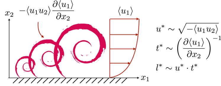
Figure 1: Sketch of wall-attached momentum-carrying eddies of different sizes in a turbulent boundary layer controlled by the mean production rate of turbulent kinetic energy, $-\langle u_{1}u_{2}\rangle\partial\langle u_{1}\rangle/\partial x_{2}$, and proposed velocity $u^{*}$, time $t^{*}$, and length $l^{*}$ scales.

The characteristic velocity scale proposed in the present work is dictated by the momentum flux

$$u^{*}\equiv\sqrt{-\langle u_{1}u_{2}\rangle}.$$ (2)

For direct comparisons with the classic scaling $u_{\tau}$, we can define an alternative characteristic velocity scale by analogy with (1) as $u^{\star}\equiv\sqrt{-\langle u_{1}u_{2}\rangle/(1-x_{2}/h)}$ (Tuerke & Jiménez, 2013). Note that the factor $\sqrt{1-x_{2}/h}$ in the definition of $u^{\star}$ is introduced only for convenience and such that $u^{\star}$ collapses to $u_{\tau}$ for a channel flow driven by a constant mean pressure gradient.

The scenario proposed for the characteristic time and length scales of wall-attached eddies also differs from the classic theory. Let us consider a momentum-carrying eddy of size $l^{*}\sim u^{*}\cdot t^{*}$ controlled by the injection of energy from the mean shear and, therefore, with characteristic lifespan

$$t^{*}\equiv\left(\frac{\partial\langle u_{1}\rangle}{\partial x_{2}}\right)^{-1}.$$ (3)

The scaling in (3) can also be interpreted as the average time for the eddies to extract energy from the mean shear. Considering the scaling proposed for $u^{*}$ in (2), the characteristic length scale is

$$l^{*}\equiv u^{*}\cdot t^{*}=\sqrt{-\langle u_{1}u_{2}\rangle}\left(\frac{\partial\langle u_{1}\rangle}{\partial x_{2}}\right)^{-1}.$$ (4)

Equation (4) can also be obtained by assuming that the momentum-carrying eddies are controlled by the mean production rate of turbulent kinetic energy, $P=-\langle u_{1}u_{2}\rangle\partial\langle u_{1}\rangle/\partial x_{2}\sim u^{*3}/l^{*}$, which together with (2) yields an expression identical to (4).

For the particular case of a plane channel flow with no-slip walls and constant mean pressure gradient we recover $u^{\star}=u_{\tau}$ away from the wall. Moreover, at high Reynolds numbers, the characteristic length $l^{*}$ in the log-region of the flow ($x_{2}\lesssim 0.2h$) with mean shear $\partial\langle u_{1}\rangle/\partial x_{2}=u_{\tau}/(\kappa x_{2})$ reduces to

$$l^{*}=u_{\tau}\sqrt{1-x_{2}/h}\left(\frac{u_{\tau}}{\kappa x_{2}}\right)^{-1}=\kappa x_{2}\sqrt{1-x_{2}/h}\approx\kappa x_{2},$$ (5)

which is proportional to the distance to the wall as commonly discussed in the literature. Therefore, the extension of the characteristic scales proposed above collapses to Townsend’s model for a canonical case. It is important to remark that despite the fact that the velocity and length scales specified by $u^{\star}$ and $l^{*}$ coincide with their classic counterparts $u_{\tau}$ and $x_{2}$ for the traditional channel flow, the former are conceptually different as they remain agnostic to the location of the wall.

3 Turbulent channel driven by $x_{2}$-dependent body force

3.1 Numerical scheme and computational domain

We perform a set of DNS of plane turbulent channel flows by solving the incompressible Navier-Stokes equations with a staggered, second-order, finite difference (Orlandi, 2000) and a fractional-step method (Kim & Moin, 1985) with a third-order Runge-Kutta time-advancing scheme (Wray, 1990). Periodic boundary conditions are imposed in the streamwise and spanwise directions, and no-slip at the walls. The code has been validated in previous studies in turbulent channel flows (Lozano-Durán & Bae, 2016; Bae et al., 2018a, b) and flat-plate boundary layers (Lozano-Durán et al., 2018).

Wall units are denoted by the superscript $+$ and defined in terms of the kinematic viscosity $\nu$ and friction velocity at the wall $u_{\tau}$. Accordingly, the friction Reynolds number is $Re_{\tau}=u_{\tau}h/\nu$. Velocities normalised by $u^{*}$ and $u^{\star}$ are denoted by the superscript $*$ and $\star$, respectively. Fluctuating quantities with respect to the mean are represented by $(\cdot)^{\prime}$. The computational domain for the present simulations is $2\pi h\times 2h\times\pi h$ in the streamwise, wall-normal, and spanwise directions, respectively. It has been shown that this domain size is large enough to accurately predict one-point turbulent statistics for $Re_{\tau}$ up to 4200 (Lozano-Durán & Jiménez, 2014a).

We compare our results with DNS data from del Álamo & Jiménez (2003) and Hoyas & Jiménez (2006) at $Re_{\tau}\approx 550,950$, and $2000$, which are labelled as NS550, NS950, and NS2000, respectively. The three cases have computational domains equal to $8\pi h\times 2h\times 3\pi h$ in the streamwise, wall-normal, and spanwise directions, respectively.

3.2 Numerical experiments of channels driven by $x_{2}$-dependent body force

We devise two sets of conceptual numerical experiments to unravel the characteristic scales of the outer-layer motions. The first set of experiments is a channel flow with no-slip walls driven by a $x_{2}$-dependent body force per unit mass of the form

$$f_{1}=\frac{u_{\tau}^{2}}{h}\left[1+\epsilon\left(2x_{2}/h-x_{2}^{2}/h^{2}\right)-2/3\epsilon\right],\ f_{2}=0,\ f_{3}=0,$$ (6)

where $f_{i}$ is the component of the force in the $i$-th direction, and $\epsilon$ is a non-dimensional adjustable parameter. Equation (6) is such that $Re_{\tau}$ remains unchanged with $\epsilon$. For $\epsilon=0$, we recover the constant body force typically used to drive the channel, $f_{1}=u_{\tau}^{2}/h$. The goal of (6) is to alter the natural balance between eddies, which are forced to readjust their intensities to accommodate the new momentum flux. Two cases are considered at $Re_{\tau}\approx 550$: $\epsilon=4$, labelled as NS550-p, and $\epsilon=-2$, labelled as NS550-n, where NS denotes no-slip boundary condition at the walls. Note that case NS550 corresponds to $\epsilon=0$.

The second set of experiments intends to clarify the characteristic length scales of the active energy-containing eddies. The change in $u^{*}$ and $t^{*}$ from NS550-p and NS550-n is not significant enough to assess conclusively the scaling proposed in (4). For that reason, two new simulations, NS550-s1 and NS550-s2, are considered by prescribing a synthetic mean velocity profile of the form

$$\frac{\langle u_{1}\rangle}{u_{\mathrm{ref}}}=\frac{\alpha+2}{\alpha+1}\left[1-(x_{2}/h-1)^{\alpha+1}\right]+\frac{\beta+2}{\beta+1}\left[1-(x_{2}/h-1)^{\beta+1}\right],$$ (7)

with $(\alpha,\beta)=(41,11)$ and $(3,3)$ for NS550-s1 and NS550-s2, respectively. The parameter $u_{\mathrm{ref}}$ was adjusted to achieve $Re_{\tau}\approx 550$. The profiles from (7) are purposely tailored to create distinguishable $l^{*}$ with values equal to $0.06h$, $0.03h$, and $0.04h$ at $x_{2}=0.10h$, for cases NS550, NS550-s1, and NS550-s2, respectively. These last two simulations are similar to channel flows driven by $x_{2}$-dependent body forces discussed above, in the sense that prescribing the mean velocity profile is equivalent to imposing a $x_{2}$-dependent (and time-dependent) forcing as in (6). Simulations of turbulent channels with prescribed velocity profiles can also be found in Tuerke & Jiménez (2013). All the cases above are designed such that $u_{\tau}$ and $x_{2}$ remain unchanged but do not coincide with the scaling proposed by $u^{\star}$ and $l^{*}$, in contrast with the traditional channel flow, where $u^{\star}\approx u_{\tau}$ and $l^{*}\approx\kappa x_{2}$. This will allow us to assess the validity of each scaling. The list of cases is summarised in table 1. All the simulations were run for at least 10 eddy turnover times (defined as $h/u_{\tau}$) after transients.

Case	$\Rey_{\tau}$	$\Delta x_{1}^{+}$	$\Delta x^{+}_{2,\mathrm{min}/\mathrm{max}}$	$\Delta x_{3}^{+}$	Driven by
NS550-p	546	6.7	0.2/9.9	3.3	$f_{1}$ with $\epsilon=4$
NS550-n	546	6.7	0.2/9.9	3.3	$f_{1}$ with $\epsilon=-2$
NS550-s1	531	6.5	0.2/9.7	3.2	prescribed $\langle u_{1}\rangle$
NS550-s2	546	6.7	0.2/9.9	3.3	prescribed $\langle u_{1}\rangle$

Table 1: Tabulated list of cases for §3. The numerical experiments are labelled following the convention NS[$\Rey_{\tau}$]-[specific case], where NS denotes channel with no-slip walls. $\Delta x_{1}$, $\Delta x_{2}$ and $\Delta x_{3}$ are the streamwise, wall-normal, and spanwise grid resolutions, respectively. The last column shows the method employed to drive the channel flow. See text for details.

3.3 Assessment of characteristic velocity and length scales

We examine scaling (2) in turbulent channel flows driven by (6). The imposed $x_{2}$-dependent body force breaks the global velocity scale with $u_{\tau}$, and the new balance for the mean momentum flux requires that

$$\langle u_{1}u_{2}\rangle\approx\int_{0}^{x_{2}}f_{1}(x^{\prime}_{2})\mathrm{d}x^{\prime}_{2}.$$ (8)

The total stresses consistent with (8) for cases NS550-p and NS550-n are shown in figure 2(a). Changes in the momentum flux propagate to the mean velocity profile as dictated by the integrated streamwise mean momentum equation, and the resulting profiles are shown in figure 2(b).

\psfrag{X}{$x_{2}/h$}\psfrag{Y}[cb]{$-\langle u_{1}^{+}u_{2}^{+}\rangle+\partial\langle u_{1}^{+}\rangle/\partial x_{2}^{+}$}\includegraphics[width=199.4681pt]{figures/uvtotal_550_eps42.eps}

(a)

\psfrag{X}{$x_{2}/h$}\psfrag{Y}[cb]{$-\langle u_{1}^{+}u_{2}^{+}\rangle+\partial\langle u_{1}^{+}\rangle/\partial x_{2}^{+}$}\psfrag{X}{$x_{2}^{+}$}\psfrag{Y}{$\langle u_{1}^{+}\rangle$}\includegraphics[width=199.4681pt]{figures/Umean_550_eps42.eps}

(b)

\psfrag{X}{$x_{2}/h$}\psfrag{Y}{$\langle{u_{i}^{\prime}}^{2+}\rangle^{1/2}$}\includegraphics[width=199.4681pt]{figures/rms_550_utau.eps}

(c)

\psfrag{X}{$x_{2}/h$}\psfrag{Y}{$\langle{u_{i}^{\prime}}^{2+}\rangle^{1/2}$}\psfrag{X}{$x_{2}/h$}\psfrag{Y}{$\langle{u_{i}^{\prime}}^{2\star}\rangle^{1/2}$}\includegraphics[width=199.4681pt]{figures/rms_550_utaun.eps}

(d)

Figure 2: Mean (a) total tangential Reynolds stress and (b) streamwise velocity profile for NS550 (            ), NS550-p ($\circ$), and NS550-n (•). Panels (c) and (d) contain the streamwise (circles and            ), wall-normal (triangles and                   ), and spanwise (squares and            ) root-mean-squared velocity fluctuations scaled with (c) $u_{\tau}$ and (d) $u^{\star}$. Symbols are for NS550-p (open) and NS550-n (closed). Lines without symbols are for NS550. For clarity, the profiles for the wall-normal and spanwise root-mean-squared velocity fluctuations are shifted vertically by 2.0 and 3.4 wall units.

The three root-mean-squared (r.m.s.) fluctuating velocities for NS550, NS550-p, and NS550-n are reported in figure 2(c). The pronounced lack of collapse among the three cases exposes the unsatisfactory scaling with $u_{\tau}$. Conversely, when the r.m.s. fluctuating velocities are scaled with $u^{\star}$, which can be analytically evaluated for cases NS550-p and NS550-n, the agreement is excellent (figure 2d). Appendix A shows results using $u^{*}$, which does not have any explicit functional dependence on $x_{2}$. Note that the argument above holds for Townsend’s active motions, i.e., those responsible for the mean momentum transfer, and that the inactive motions are not expected to scale with $u^{\star}$ (or $u^{*}$) but with the bulk velocity or a mixed scale as suggested in previous works (Zagarola & Smits, 1998; De Graaff & Eaton, 2000; del Álamo et al., 2004; Morrison et al., 2004).

Scaling (4) is investigated in cases NS550, NS550-s1, and NS550-s2 with mean velocity profiles shown in figure 3(a). Figure 3(b) contains the tangential Reynolds stress artificially generated to sustain $\langle u_{1}\rangle$.

\psfrag{X}{$x_{2}^{+}$}\psfrag{Y}{$\langle u_{1}^{+}\rangle$}\includegraphics[width=199.4681pt]{figures/Umean_550_Ufixed.eps}

(a)

\psfrag{X}{$x_{2}^{+}$}\psfrag{Y}{$\langle u_{1}^{+}\rangle$}\psfrag{X}{$x_{2}/h$}\psfrag{Y}[cb]{$-\langle u_{1}^{+}u_{2}^{+}\rangle$}\includegraphics[width=199.4681pt]{figures/uv_550_Ufixed.eps}

(b)

Figure 3: Mean (a) streamwise velocity profile and (b) tangential Reynolds stress for NS550 (            ), NS550-s1 ($\circ$), and NS550-s2 (•). The dash-dotted line is $x_{2}=0.1h$.

The relevant length scale of the momentum-carrying eddies is examined in figure 4 by comparing the premultiplied, two-dimensional velocity spectra at $x_{2}=0.10h$ as a function of the streamwise and spanwise wavelengths ($\lambda_{1}$ and $\lambda_{3}$) scaled by the distance to the wall (top panels) and $l^{*}$ (bottom panels). The spectra display a noticeable mismatch when the wavelengths are scaled by $x_{2}$, whereas the collapse is appreciably improved when $\lambda_{1}$ and $\lambda_{3}$ are normalised by $l^{*}$, especially for the most intense spectral cores. Therefore, $l^{*}$ stands as a more faithful characterisation of the eddy sizes compared to the distance to the wall.

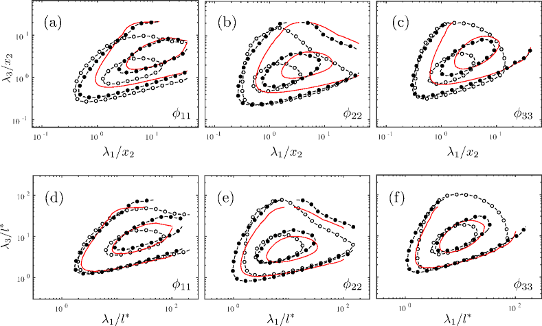
Figure 4: Premultiplied streamwise $\phi_{11}$ (a,d), wall-normal $\phi_{22}$ (b,e), and spanwise $\phi_{33}$ (c,f) velocity two-dimensional spectra at $x_{2}=0.10h$ for NS550 (   ), NS550-s1 ($\circ$), and NS550-s2 (•). The wavelengths are scaled by $x_{2}$ in the top panels and by $l^{*}$ in the bottom panels. Contours are 0.1 and 0.6 of the maximum.

We further examine the performance of $l^{*}$ at different wall-normal heights using the traditional channel flow NS2000. Figure 5 shows the premultiplied velocity spectra for multiple wall-normal distances ranging from $x_{2}=0.1h$ to $x_{2}=0.4h$. We test three different length scales to normalise the streamwise and spanwise wavelengths, namely, $h$ (figures 5 a,b,c), $x_{2}$ (figures 5 d,e,f), and $l^{*}$ (figures 5 g,h,i). Again, the best collapse is attained for $l^{*}$, although $x_{2}$ also provides a quantitative improvement with respect to $h$.

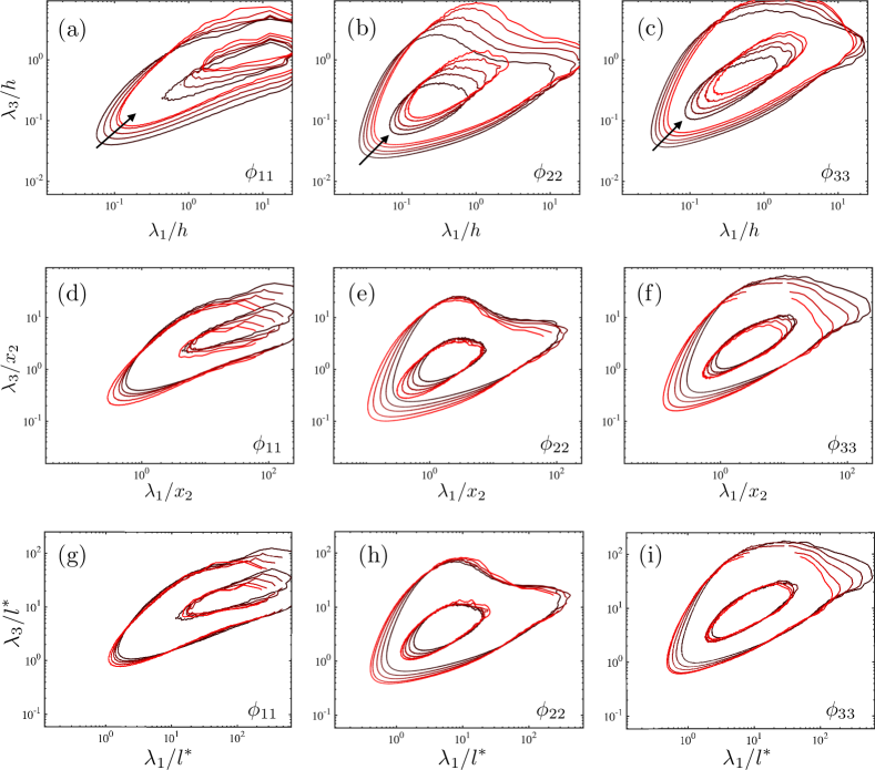
Figure 5: Premultiplied streamwise $\phi_{11}$ (a,d,g), wall-normal $\phi_{22}$ (b,e,h), and spanwise $\phi_{33}$ (c,f,i) two-dimensional velocity spectra at $x_{2}/h=0.10,0.15,0.20,0.30$ and $0.40$ (from black to red) for NS2000. The wavelengths are scaled by $h$ (a,b,c), $x_{2}$ (d,e,f), and $l^{*}$ (g,h,i). Contours are 0.1 and 0.6 of the maximum. The arrows in panels (a), (b), and (c) indicate increasing distance from the wall.

The normalisation by $l^{*}$ is still far from perfect, although this may be expected considering that the new scaling is only applicable to the active motions responsible for carrying the tangential momentum flux. For that reason, both the lower spectral contours and the large-scale tails of $\phi_{11}$ and $\phi_{33}$ are not required to scale with $l^{*}$, the former due to contamination from small eddies decoupled from the mean shear, and the latter due to their lack of tangential stress despite their non-zero energy content.

In summary, we have shown that $u^{*}$ (or $u^{\star}$) and $l^{*}$ are tenable candidates to represent the characteristic scales of the momentum-carrying eddies in wall-bounded turbulence. Although we have focused on channel flows, we expect $u^{*}$ and $l^{*}$ to perform similarly in turbulent boundary layers. The proposed scales are still consistent with the classic scaling provided by $u_{\tau}$ and $x_{2}$ for canonical flows, and can be considered as an extension for more general shear-dominated turbulence.

4 Turbulent channel with Robin boundary conditions

In this section, we analyse the significance of the distance to the wall for the outer flow by using turbulent channel flows where the no-slip wall is replaced by Robin boundary conditions. The new set-up allows for instantaneous velocities at the boundaries and, in particular, for wall-normal transpiration. No transpiration is considered to be the most distinctive feature of walls, and it is commonly understood as the mean by which the log-layer motions “feel” the distance to the wall. Hence, the non-zero $u_{2}$ at $x_{2}=0$ (and $x_{2}=2h$) introduced by the Robin boundary condition is intended to assess the role of impermeable walls as organising agents of wall-attached eddies.

4.1 Numerical experiments of channels with Robin boundary conditions

We perform a set of DNS of turbulent channel flows using the same numerical scheme and computational domain from §3.1. The no-slip wall is replaced by a Robin boundary condition of the form

$$u_{i}|_{w}=l\left.\frac{\partial u_{i}}{\partial n}\right|_{w},\quad i=1,2,3,$$ (9)

where the subscript $w$ refers to quantities evaluated at the wall, and $n$ is the wall-normal (or boundary-normal) direction. We define $l$ to be the slip length that, in general, may be a function of the spatial wall-parallel coordinates and time. The choice of $l$ must comply with the symmetries of the flow and, particularly for a channel flow configuration, (9) should satisfy

$$\langle u_{i}|_{w}\rangle=\left\langle\left.l\frac{\partial u_{i}}{\partial x_{2}}\right|_{w}\right\rangle=0,\quad i=2,3.$$ (10)

In the present study, we consider a constant value for $l$. This is consistent with (10) because $\langle u_{i}|_{w}\rangle=0$ and $\left.\left\langle{\partial u_{i}}/{\partial x_{2}}\right|_{w}\right\rangle=0$ for $i=2,3$. The cases simulated are summarised in table 2. All the simulations were run for at least 10 eddy turnover times after transients. Throughout the text, we occasionally refer to cases with the Robin boundary condition as Robin-bounded and those with the no-slip condition as wall-bounded. Robin boundary conditions have been previously employed in the wall-parallel directions to model the flow over hydrophobic surfaces (Min & Kim, 2004; Martell et al., 2009; Park et al., 2013; Jelly et al., 2014; Seo et al., 2015; Seo & Mani, 2016), but note that in the present study the boundary condition is also applied to the wall-normal velocity, which is seldom done in the literature. The slip lengths used here are also larger than the typical values in hydrophobic works.

Case	$\Rey_{\tau}$	$\Delta x_{1}^{+}$	$\Delta x^{+}_{2,\mathrm{min}/\mathrm{max}}$	$\Delta x_{3}^{+}$	$l/h$	Driven by
R550	546	6.7	0.2/9.9	3.3	0.10	constant $\langle\frac{\mathrm{d}p}{\mathrm{d}x_{1}}\rangle$
R550-l1	546	6.7	0.2/9.9	3.3	0.25	constant $\langle\frac{\mathrm{d}p}{\mathrm{d}x_{1}}\rangle$
R550-l2	546	6.7	0.2/9.9	3.3	0.50	constant $\langle\frac{\mathrm{d}p}{\mathrm{d}x_{1}}\rangle$
R950	934	5.7	0.5/10.1	2.8	0.10	constant $\langle\frac{\mathrm{d}p}{\mathrm{d}x_{1}}\rangle$
R2000	2003	6.1	0.7/15.0	3.1	0.10	constant $\langle\frac{\mathrm{d}p}{\mathrm{d}x_{1}}\rangle$

Table 2: Tabulated list of cases for §4. The numerical experiments are labelled following the convention R[$\Rey_{\tau}$]-[specific case], where R denotes channel with Robin boundary condition. $\Delta x_{1}$, $\Delta x_{2}$ and $\Delta x_{3}$ are the streamwise, wall-normal, and spanwise grid resolutions, respectively. The slip length used in the Robin boundary condition is $l$. The last column shows the method employed to drive the channel flow. See text for details.

The motivation of using (9) is to provide a boundary for the flow that deviates from the behaviour of a regular wall. Indeed, for large values of $l$, (9) constitutes a significant modification of the classic no-slip boundary condition by suppressing the formation of near-wall viscous layers (Lozano-Durán & Bae, 2016). The mean tangential Reynolds stress is shown in figure 6(a) for cases R550, R950, and R2000 with slip length $l=0.10h$. For the three Reynolds numbers under consideration, $-\langle u_{1}u_{2}\rangle$ captures more than 90% of the total stress, and this was the criteria used to select $l=0.10h$ as the reference slip length. As the Reynolds number increases, so does the contribution of $-\langle u_{1}u_{2}\rangle$ close to the wall at the expense of reducing the formation of near-wall viscous layers that appear prior to the proximity of the wall. Far from the boundaries, the tangential momentum flux is linear for the same reason as in wall-bounded channels, i.e., to balance the constant mean pressure gradient driving the flow. Cases R550-l1 and R550-l2 are for $l=0.25h$ and $l=0.50h$, respectively, and are intended to test the effect of increasing slip lengths.

\psfrag{X}{$x_{2}^{+}$}\psfrag{Y}{$-\langle u_{1}^{+}u_{2}^{+}\rangle$}\includegraphics[width=195.12767pt]{figures/uvmean_log.eps}

(a)

\psfrag{X}{$x_{2}^{+}$}\psfrag{Y}{$-\langle u_{1}^{+}u_{2}^{+}\rangle$}\psfrag{X}{$\lambda_{1}/h$}\psfrag{Y}{$\lambda_{3}/h$}\includegraphics[width=203.80193pt]{figures/spectra_Res-plane-1_var-2_DNS.eps}

(b)

Figure 6: (a) Mean tangential Reynolds stress as a function of the wall-normal coordinate for R550 ($\circ$), R950 ($\blacktriangledown$), R2000 ($\square$), NS550 (            ), NS950 (                ), and NS2000 (            ). (b) Premultiplied wall-normal two-dimensional velocity spectra for Robin-bounded channels at $x_{2}/h=0$. Contours are 0.1 and 0.6 of the maximum. The red dashed lines are $\lambda_{1}/h=1$ and $\lambda_{3}/h=1$. Symbols are as in (a).

Another two important properties of the Robin boundary condition are that it allows for transpiration at all flow scales and, it does not encode any specific information regarding the linear wall-normal scaling of the log-layer eddies. The spectral density of the wall-normal velocity, $\phi_{22}$, evaluated at $x_{2}/h=0$ for Robin-bounded cases is shown in figure 6(b) as a function of the streamwise and spanwise wavelengths, $\lambda_{1}$ and $\lambda_{3}$, respectively. The spectra are non-zero at the boundary with a non-negligible contribution from wavelengths up to $\lambda_{1}$ and $\lambda_{3}$ of $\mathcal{O}(h)$. Moreover, the spectral energies obtained by integrating $\phi_{22}$ at $x_{2}/h=0$ are approximately $u_{\tau}^{2}$, that is of the same order as the values in the bulk flow. This implies that the Robin boundary should alter the behaviour of eddies with sizes up to $\mathcal{O}(h)$ if they are controlled by the distance to the wall as commonly hypothesised (Townsend, 1976).

One could still argue that $\langle u_{2}|_{w}\rangle$ is zero, analogously to the scenario encountered for impermeable walls. However, note that this is also the case for $\langle u_{2}\rangle$ at each wall-normal location for a no-slip channel, and that (10), and hence $\langle u_{2}|_{w}\rangle=0$, is just the immediate consequence of the symmetries of the channel flow configuration rather than a result of the impermeability constraint. The only reminiscence of the wall in the Robin boundary condition comes from the fact that, by construction of (9), the velocities and their corresponding wall-normal derivatives are expected to show similar lengths scales in the vicinity of the wall akin to the production and dissipation in the buffer region of a smooth wall.

Instantaneous flow fields for the three velocity components at $Re_{\tau}=2000$ for NS2000 and R2000 are compared in figure 7. The similarities between both visualisations are striking, and their resemblance is confirmed by the quantitative analysis of the flow statistics presented in the following sections. Note that the Robin boundary condition is introduced in the present work just as a mean to confine the flow within a boundary which differs from a no-slip wall, especially regarding transpiration. In this sense, the Robin boundary condition is just a tool and it is not intended to model any particular flow phenomena. Moreover, the focus of this paper lies on the outer region and we are less interested in the structure of the flow at the boundary. Nonetheless, a further characterisation of the flow at $x_{2}/h=0$ is provided in Appendix B for completeness.

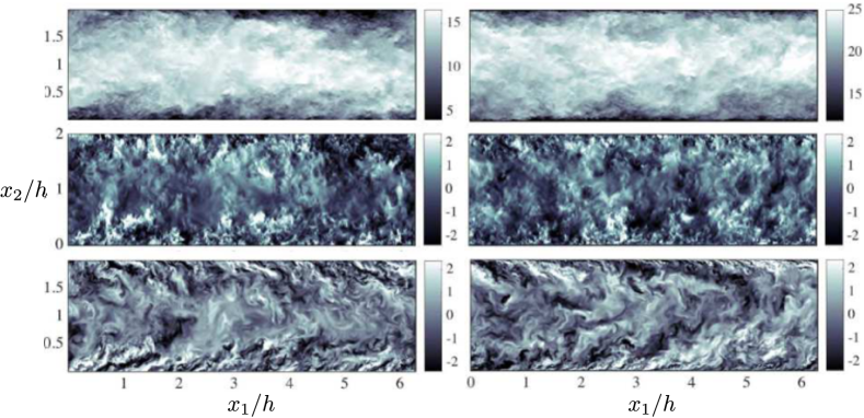
Figure 7: Instantaneous $x_{1}$–$x_{2}$ planes of the streamwise (top), wall-normal (centre), and spanwise (bottom) velocities for turbulent channels at $Re_{\tau}=2000$. Left panels are for R2000, and right panels are for NS2000. The colour bars show velocity in wall units.

4.2 One-point statistics and spectra

The mean streamwise velocities for the Robin-bounded and wall-bounded channel flows are compared in figure 8. In figure 8(b), the mean profiles for Robin-bounded cases are vertically displaced to match the centreline velocity of the corresponding no-slip case. A first observation is that the shape of $\langle u_{1}\rangle$ remains roughly identical for $x_{2}\gtrsim 0.10h$, and the Robin boundary condition is mainly responsible for a reduction of the total mass flux. The shifts required to match the Robin-bounded cases to their no-slip counterpart were positive and equal to $6.4$, $8.0$, and $8.9$ plus units for R550, R950, and R2000, respectively. Nonetheless, we will not emphasise these values as they can be trivially changed by either adding a constant uniform velocity to the right-hand side of the Robin boundary condition (9), or by a Galilean transformation of the velocity field.

The observations from figure 8 can be connected to the law of the wall (Prandtl, 1925; von Kármán, 1930; Millikan, 1938; Townsend, 1976),

$$\langle u_{1}^{+}\rangle=\frac{1}{\kappa}\log\left(x_{2}^{+}\right)+B+\Pi,$$ (11)

where $\kappa$ and $B$ are the von Kármán and intercept constants for no-slip walls, respectively, and $\Pi$ is an additional velocity displacement. The friction velocity for Robin-bounded cases is $u_{\tau}=\sqrt{\nu\partial\langle u_{1}\rangle/\partial x_{2}-\langle u_{1}u_{2}\rangle}|_{x_{2}=0}$. Hence, the Robin boundary condition introduces a non-zero tangential Reynolds stress at the wall, which acts as an effective drag with a major impact on $\Pi$ (see Nikuradse, 1933; Jiménez, 2004). On the hand, we can hypothesise that the $x_{2}$-dependent component, $\sim 1/\kappa\log(x_{2})$, is mainly controlled by the momentum flux for $x_{2}>0$.

\psfrag{X}[br]{$x_{2}/h$}\psfrag{Y}{$\langle u_{1}^{+}\rangle$}\includegraphics[width=203.80193pt]{figures/Umean.eps}

(a)

\psfrag{X}[br]{$x_{2}/h$}\psfrag{Y}{$\langle u_{1}^{+}\rangle$}\psfrag{X}[br]{$x_{2}^{+}$}\psfrag{Y}{$\langle u_{1}^{+}\rangle-u_{1}^{\mathrm{shift}}$}\includegraphics[width=203.80193pt]{figures/Umean_shifted.eps}

(b)

Figure 8: Mean streamwise velocity profiles as a function of $x_{2}$ in (a) linear scale and (b) logarithmic scale for R550 ($\circ$), R950 ($\triangledown$), R2000 ($\square$), NS550 (            ), NS950 (                ), and NS2000 (            ). In panel (b), the velocity profiles of Robin-bounded cases are vertically shifted such that centreline velocity coincide with their corresponding wall-bounded case. For clarity, profiles at $Re_{\tau}\approx 950$ and $Re_{\tau}\approx 2000$ are additionally shifted by 5 and 10 plus units, respectively.

The r.m.s. velocity fluctuations for the Robin-bounded and wall-bounded channels are shown in figure 9(a–c). The lack of a near-wall peak at $x_{2}^{+}\approx 15$ for the Robin-bounded streamwise velocity fluctuations is a consequence of the interruption of the classic near-wall cycle (Jiménez & Moin, 1991; Jiménez & Pinelli, 1999), which is also confirmed by visual inspection of the instantaneous near-wall velocities (see Appendix B). The most remarkable observation from figure 9 is that the Robin-bounded fluctuating velocities match quantitatively their wall-bounded counterparts for $x_{2}\gtrsim 0.10h$ despite the lack of impermeable walls. The presence of a significant non-zero $u_{2}$ in the Robin-bounded cases is evidenced by the r.m.s. of $u_{2}$ at $x_{2}/h=0$ whose values are comparable to the r.m.s. in the bulk flow. The result is again an indication that the total contribution of the different eddies to the turbulence intensities is insensitive to the presence of impermeable walls. The pressure fluctuations are also accurately reproduced in figure 9(d) for the Robin-bounded cases. The results may appear surprising due to the global nature of the pressure, which is more prone to being affected by the changes in the boundary condition. However, the most important contribution of the pressure is to guarantee local continuity among eddies, and the satisfactory collapse of the r.m.s. velocity fluctuations seen in figures 9(a–c) also imply equally fair results for the pressure fluctuations. This is in accordance with Sillero et al. (2014), who concluded from the pressure correlations in boundary layers that $p$ is dominated by localised regions of strongly coupled small-scale structures.

\psfrag{X}[cr]{$x_{2}/h$}\psfrag{Y}{$\langle{u_{1}^{\prime}}^{2+}\rangle^{1/2}$}\includegraphics[width=208.13574pt]{figures/urms.eps}

(a)

\psfrag{X}[cr]{$x_{2}/h$}\psfrag{Y}{$\langle{u_{1}^{\prime}}^{2+}\rangle^{1/2}$}\psfrag{X}[cr]{$x_{2}/h$}\psfrag{Y}{$\langle{u_{2}^{\prime}}^{2+}\rangle^{1/2}$}\includegraphics[width=208.13574pt]{figures/vrms.eps}

(b)

\psfrag{X}[cr]{$x_{2}/h$}\psfrag{Y}{$\langle{u_{3}^{\prime}}^{2+}\rangle^{1/2}$}\includegraphics[width=208.13574pt]{figures/wrms.eps}

(c)

\psfrag{X}[cr]{$x_{2}/h$}\psfrag{Y}{$\langle{u_{3}^{\prime}}^{2+}\rangle^{1/2}$}\psfrag{X}[cr]{$x_{2}/h$}\psfrag{Y}{$\langle{p^{\prime}}^{2+}\rangle^{1/2}$}\includegraphics[width=208.13574pt]{figures/prms.eps}

(d)

Figure 9: (a) Streamwise, (b) wall-normal, and (c) spanwise root-mean-squared velocity fluctuations, and (d) root-mean-squared pressure fluctuations for R550 ($\circ$), R950 ($\triangledown$), R2000 ($\square$), NS550 (            ), NS950 (                ), and NS2000 (            ). In all panels, the profiles for cases at $Re_{\tau}\approx 950$ and $Re_{\tau}\approx 2000$ are vertically shifted by $0.5$ and $1$ plus units, respectively, for clarity.

The spectral densities of the three velocity fluctuations, $\phi_{11}$, $\phi_{22}$, and $\phi_{33}$, are shown in figure 10 as a function of the streamwise and spanwise wavelengths. Several wall-normal heights are considered for R2000 and NS2000. The spectra for wall-bounded cases is zero at $x_{2}/h=0$. Conversely, $\phi_{22}$ is non-zero at the boundary for the Robin-bounded case, and peaks at $\lambda_{1}\approx 0.3h$ and $\lambda_{3}\approx 0.10h$, with a non-negligible contribution from wavelengths up to $\lambda_{1}$ and $\lambda_{3}$ of $\mathcal{O}(h)$. We can then estimate the flow scales that are expected to be affected by the transpiration of the boundary by assuming that the stress-carrying eddies follow $\lambda_{1}\approx 1.5x_{2}$ and $\lambda_{3}\approx x_{2}$ (as shown below in §4.5). If the boundary is perceived as permeable for scales up to $\mathcal{O}(h)$, then attached motions below $x_{2}\approx 0.7h$ should adjust accordingly to accommodate transpiration effects, especially if the wall is their primary organising agent. However, inspection of the spectra above $x_{2}\approx 0.10h$ shows that the agreement between wall-bounded and Robin-bounded channels is outstanding (figures 10 b,c,e,f,h,i). Consequently, the distance to the boundary (or non-existent wall) is not the relevant length scale controlling the size of the attached eddies, in contrast with the traditional argument by Townsend (1976). Instead, the resemblance between wall-bounded and Robin-bounded cases presented above should be attributed to the common momentum transfer $u_{\tau}^{2}$ characteristic of both cases as argued in §2.

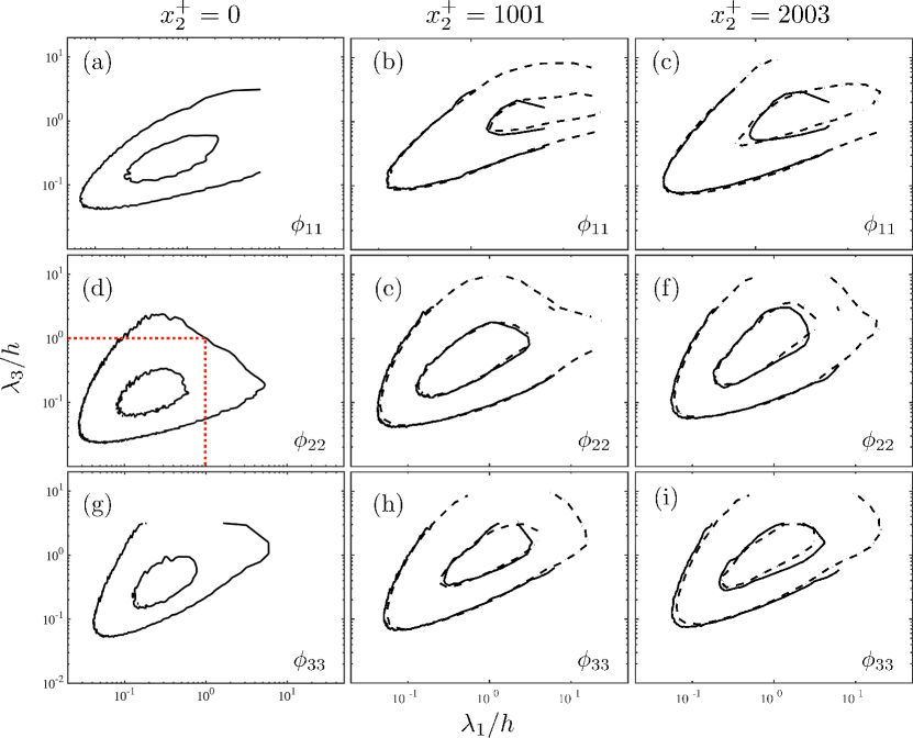
Figure 10: Wall-parallel premultiplied streamwise (a,b,c), wall-normal (d,e,f), and spanwise (g,h,i) velocity spectra for R2000 (   ) and NS2000 (            ). The wall-normal locations are $x_{2}^{+}=0$ (a,d,g), $x_{2}^{+}=1001$ (b,e,h), and $x_{2}^{+}=2003$ (c,f,i). Contours are 0.1 and 0.6 of the maximum. The red dotted lines in (d) are $\lambda_{1}/h=1$ and $\lambda_{3}/h=1$.

It also worth noting that the excellent agreement of the one-point statistics and spectra occurs in spite of the absence of very large-scale motions longer than $\sim$$6h$ (Guala et al., 2006; Balakumar & Adrian, 2007) that do not fit within the limited computational domain of the present simulations. The result is consistent with Flores & Jiménez (2010) and Lozano-Durán & Jiménez (2014a), and scales larger than $\sim$$6h$ can be essentially modelled as infinitely long (due to the streamwise periodicity of the channel) while still interacting correctly with the smaller well-resolved eddies.

4.3 Existence of a virtual wall vs. adaptation layer from the boundary

It could be still argued that the flow is influenced by an effective virtual wall whose origin is vertically displaced with respect to the boundary. In that case, different values of the slip length $l$ would be accompanied by changes in the origin of the virtual wall. The virtual-wall argument, often invoked in roughness studies (Raupach et al., 1991; Jiménez, 2004), proved not to be necessary in §4.2, where it was shown that the flow recovers above some wall-normal distance, $l_{a}$, without requiring a shift in $x_{2}$. Nevertheless, the position of the hypothetical virtual wall, $\delta x_{2}$, can be estimated by a least-square fit of the mean velocity profile to the logarithmic law (Raupach et al., 1991),

$$\langle u_{1}^{+}\rangle=\frac{1}{\kappa}\log(x_{2}^{+}-\delta x_{2}^{+})+B-\Delta\langle u_{1}^{+}\rangle,$$ (12)

with $\kappa=0.392$ and $B=4.48$ (Luchini, 2017), within the range $x_{2}\in[0.1h,0.2h]$. For this purpose, we will consider two additional cases with $l=0.25h$ and $l=0.50h$ at $Re_{\tau}\approx 550$ labelled respectively as R550-l1 and R550-l2 in table 2. The spectral density $\phi_{22}$ for the three different slip lengths is reported in figure 11(a) at $x_{2}/h=0$. As $l$ increases, the spectrum moves towards higher wavelengths along the ridge $\lambda_{1}\sim\lambda_{3}$, and transpiration is allowed for larger scales, which in principle should change the location of the virtual wall. However, the virtual wall off-set computed with (12) is $\delta x_{2}^{+}\approx\mathcal{O}(10)$ for all the Robin-bounded cases in table 2, which is not significant enough to alter in a meaningful manner the energy-containing eddies populating the log-layer. Furthermore, when the $x_{2}$ direction was remapped into $\tilde{x}_{2}=x_{2}+\delta x_{2}(1-x_{2}/h)$ (Flores & Jiménez, 2006), the collapse of the r.m.s. velocity fluctuations worsened despite the minor improvements in $\langle u_{1}\rangle$. Consequently, the results do not comply with the existence of a the virtual wall. Note that the same conclusion does not apply to the viscous eddies close to the wall with sizes comparable to $\delta x_{2}$, where changes in the permeability of the boundary are expected to have a considerable impact on the near-wall flow dynamics as typically described in flow control strategies (Choi et al., 1994; Abderrahaman-Elena & García-Mayoral, 2017).

Instead of a virtual wall, we analyse the results assuming the existence of an adaptation layer from the boundary. The vertical distance from the boundary above which the flow recovers to the nominal no-slip flow statistics, $l_{a}$, is plotted in figure 11(b) and is referred to as adaptation length. More specifically, $l_{a}$ is defined as the maximum boundary-normal distance from which

$$\mathcal{E}^{+}(x_{2})=|\psi^{+}(x_{2})-\psi^{+}_{\mathrm{NS}}(x_{2})|<\alpha,$$ (13)

where the subscript NS denotes variables for no-slip cases, and $\psi$ takes the value of $\langle u_{1}\rangle$ or $\langle{u_{i}^{\prime}}^{2}\rangle^{1/2}$ with $i=1,2,3$, depending on whether the adaptation length refers to the recovery of the mean velocity profile, or the streamwise, wall-normal or spanwise r.m.s. velocity fluctuations, respectively. The thresholding error $\alpha$ is set to be equal to 0.5 plus units for the mean profile and 0.1 for the r.m.s. velocity fluctuations. The results show that the flow statistics collapse to the corresponding no-slip channel above $l_{a}\sim l$ for the quantities assessed and various Reynolds numbers. The selected values of $\alpha$ are admittedly arbitrary and other choices may be preferred without any major consequences other than a vertical shift of the adaptation length in figure 11(b).

\psfrag{X}{$\lambda_{3}/h$}\psfrag{Y}{$\lambda_{1}/h$}\includegraphics[width=208.13574pt]{figures/spectra_550_plane-1_var-2_DNS.eps}

(a)

\psfrag{X}{$\lambda_{3}/h$}\psfrag{Y}{$\lambda_{1}/h$}\psfrag{X}{$l/h$}\psfrag{Y}{$l_{a}/h$}\includegraphics[width=208.13574pt]{figures/adaptation_lengths.eps}

(b)

Figure 11: (a) Wall-parallel premultiplied wall-normal velocity spectra at $x_{2}^{+}=0$ for R550 (   ), R550-l1 ($\circ$), and R550-l2 (•). Contours are 0.1 and 0.6 of the maximum. The red dashed line is $\lambda_{3}=0.7\lambda_{1}$. (b) Adaptation length $l_{a}$ for the mean velocity profile ($\Diamond$), and root-mean-squared streamwise ($\circ$), wall-normal ($\square$) and spanwise ($\triangledown$) velocity fluctuations as a function of the slip length $l$. Colours are black for R550, blue for R950, and red for R2000.

Then, results from figure 11(b) can be interpreted without the need of a virtual wall if the boundary condition is understood as a flow distortion stirred by the turbulent background for a depth $l_{a}^{2}\sim\nu_{t}t$ during a time period of $t\sim l_{a}/\langle u_{2}^{2}\rangle^{1/2}$, where $\nu_{t}$ is the eddy viscosity. Assuming that $\nu_{t}\sim\langle u_{1}u_{2}\rangle/\langle\partial u_{1}/\partial x_{2}\rangle$, and that the flow follows (9) within the adaptation layer defined by $x_{2}\lesssim l_{a}$, then

$$l_{a}\sim\frac{\langle u_{1}u_{2}\rangle}{\langle u_{2}^{2}\rangle^{1/2}\left\langle\frac{\partial u_{1}}{\partial x_{2}}\right\rangle}\approx l\frac{\left\langle\frac{\partial u_{1}}{\partial x_{2}}\frac{\partial u_{2}}{\partial x_{2}}\right\rangle}{\left\langle\left(\frac{\partial u_{2}}{\partial x_{2}}\right)^{2}\right\rangle^{1/2}\left\langle\frac{\partial u_{1}}{\partial x_{2}}\right\rangle},$$ (14)

from where it is reasonable to assume that $l_{a}\sim l$ in first-order approximation, consistent with the results reported in figure 11(b). The existence of this adaptation layer due to the imposition of an unphysical Robin boundary condition together with the observations from previous sections suggest that both the Robin-bounded and wall-bounded channels share identical flow motions for $x_{2}>l_{a}$ once the disturbance by the boundary vanishes.

4.4 Logarithmic layer without inner-outer scale separation

The Robin boundary condition from (9) imposes a new length scale to the eddies in the near-wall region. The characteristic flow length scales of the no-slip and Robin-bounded channels are plotted in figure 12(a) as a function of $x_{2}$. The small and large scales are represented by the Kolmogorov length scale $\eta=(\nu^{3}/\varepsilon)^{1/4}$ and the integral length scale $L_{\varepsilon}=(2k/3)^{3/2}/\varepsilon$, respectively, where $\varepsilon$ is the rate of energy dissipation and $k$ is the turbulent kinetic energy. Note that $L_{\varepsilon}$ drops rapidly to zero as $x_{2}$ approaches the wall for the no-slip channel, whereas it remains roughly constant in the Robin-bounded cases. Moreover, the comparison of $L_{\varepsilon}$ at three different $Re_{\tau}$ for the Robin-bounded channels shows that the integral length scale collapses in outer units across the entire boundary layer thickness, including the region close to $x_{2}/h=0$. These results can be read as the disruption of the classic viscous scaling of the active energy-containing eddies at the wall, i.e., their sizes are a fixed fraction of $h$ and do not decrease with $Re_{\tau}$.

\psfrag{X}[bc]{$x_{2}/h$}\psfrag{Y}[cc]{$\eta/h$, $L_{\varepsilon}/h$}\includegraphics[width=208.13574pt]{figures/scales_950.eps}

(a)

\psfrag{X}[bc]{$x_{2}/h$}\psfrag{Y}[cc]{$\eta/h$, $L_{\varepsilon}/h$}\psfrag{X}[br]{$Re_{\tau}$}\psfrag{Y}{$\mathcal{E}_{l}^{+}$}\includegraphics[width=205.97214pt]{figures/Umean_convergence_log.eps}

(b)

Figure 12: (a) Kolmogorov length scale $\eta$ for NS550 (            ) and R550 ($\circ$), and integral length scale $L_{\varepsilon}$ for NS550 (   ), R550 ($\square$), R950 ($\Diamond$), and R2000 ($\triangle$). (b) $\mathcal{E}_{l}$ as a function of $Re_{\tau}$. Closed and open symbols are for wall-bounded and Robin-bounded cases, respectively. The dashed line is $\mathcal{E}_{l}^{+}\sim Re_{\tau}^{-1}$.

In spite of the lack of inner-outer layer scale separation with increasing $Re_{\tau}$, the mean velocity profile for Robin-bounded cases (figure 8a) tends towards a log-layer as in wall-bounded channels. This is quantified in figure 12(b), which contains the error function

$$\mathcal{E}_{l}^{+}=\left[\frac{1}{0.1}\int_{0.1}^{0.2}\left(x_{2}^{+}\frac{\partial\langle u_{1}^{+}\rangle}{\partial x_{2}^{+}}-\frac{1}{\kappa}-\frac{x_{2}}{h}\right)^{2}\mathrm{d}(x_{2}/h)\right]^{1/2},$$ (15)

with $\kappa=0.384$ (Lee & Moser, 2015) as a function of $Re_{\tau}$. Equation (15) measures the deviation of $x_{2}^{+}\partial\langle u_{1}^{+}\rangle/\partial x_{2}^{+}$ with respect to its asymptotic value for a well-developed log-layer, $1/\kappa-x_{2}/h$, within the range $x_{2}/h\in[0.1,0.2]$. The asymptotic value of $x_{2}^{+}\partial\langle u_{1}^{+}\rangle/\partial x_{2}^{+}$ has been derived by several authors using matched asymptotic expansions (Mellor, 1972; Afzal & Yajnik, 1973; Afzal, 1976; Phillips, 1987; Jiménez & Moser, 2007),

$$x_{2}^{+}\frac{\partial\langle u_{1}^{+}\rangle}{\partial x_{2}^{+}}\approx\frac{1}{\kappa}+\frac{x_{2}}{h}+\frac{\tilde{\beta}}{Re_{\tau}},$$ (16)

with $\tilde{\beta}$ a Reynolds-number-independent constant. The results, plotted in figure 12(b), show that $\mathcal{E}_{l}$ is larger for Robin-bounded cases than for wall-bounded cases, but both set-ups converge to the expected value at a rate close to $Re_{\tau}^{-1}$ as predicted by (16). The fact that Robin-bounded cases approach a logarithmic profile for increasing $Re_{\tau}$ without the inner-outer scale separation challenges the log-layer formulations derived from Millikan’s argument (see Millikan, 1938; Wosnik et al., 2000; Oberlack, 2001; Buschmann & Gad-el Hak, 2003, among others). Nonetheless, the Reynolds numbers in the present work are too low to attain a well-developed log-layer, and therefore, the results are indicative but not conclusive of the convergence of Robin-bounded cases to an actual wall-bounded log-layer. As we are concerned with the outer layer, the analysis above was performed for a range of wall-normal distances fixed in outer units, $x_{2}/h\in[0.1,0.2]$, and the slip length set to a given fraction of $h$. The effect of keeping the slip length constant in wall units as $Re_{\tau}$ increases is discussed in Appendix C, where we show the development of the log-layer in the wall-normal direction.

4.5 Wall-attached eddies without walls

A more detailed analysis of the size of the eddies is provided by the investigation of three-dimensional regions of the flow where a quantity of interest is particularly intense. We focus on the regions of high momentum transfer from Lozano-Durán et al. (2012) (see also Lozano-Durán & Jiménez, 2014b; Lozano-Durán & Borrell, 2016), defined as spatially connected points in the flow satisfying

$$-{u_{1}^{\prime}}{u_{2}^{\prime}}>H\langle{u_{1}^{\prime}}^{2}\rangle^{1/2}\langle{u_{2}^{\prime}}^{2}\rangle^{1/2},$$ (17)

where ${u_{1}^{\prime}}{u_{2}^{\prime}}$ is the instantaneous point-wise fluctuating tangential Reynolds stress, and $H$ is a thresholding parameter equal to $1.75$ obtained from a percolation analysis (Moisy & Jiménez, 2004). Three-dimensional structures are then constructed by connecting neighbouring grid points fulfilling relation (17) and using the 6-connectivity criteria (Rosenfeld & Kak, 1982). The cases under investigation are NS2000 and R2000, and the total number of structures identified is of the order of $10^{6}$. Since we are interested in the outer-layer eddies, the region $x_{2}^{+}<100$ was excluded from case NS2000 in order to avoid spurious contributions from the viscous layer that are not present in R2000. This is consistent with Dong et al. (2017), who showed that objects identified by (17) are artificially elongated in the streamwise direction when the region below $x_{2}^{+}=100$ is included.

Figure 13 shows two examples of actual objects extracted from NS2000 and R2000, and underlines the complex geometries that may arise. Although visual impressions should not substitute statistical analysis, the comparison between the two examples reinforces the idea that the structures in Robin-bounded and wall-bounded channels are comparatively similar.

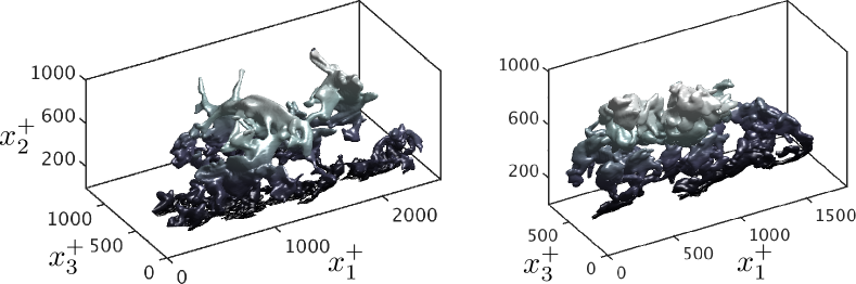
Figure 13: Example of instantaneous three-dimensional momentum transfer structures extracted from R2000 (left) and NS2000 (right). The mean flow is from bottom left to top right. Axes are normalised in plus units. The colour gradient indicates distance to the wall/boundary.

Lozano-Durán et al. (2012) and Lozano-Durán & Jiménez (2014b) showed that objects defined by (17) are responsible for most of the momentum transfer in the log-layer, justifying the choice of intense regions of $u_{1}^{\prime}u_{2}^{\prime}$ as representative structures of the flow. Moreover, these regions are geometrically and temporally self-similar and can be considered as sensible contenders for the active wall-attached eddies envisioned by Townsend (1976). Therefore, it is interesting to compare the geometry of these structures in wall-bounded and Robin-bounded channel flows. The sizes of the objects are measured by circumscribing each structure within a box aligned to the Cartesian axes, whose streamwise, wall-normal and spanwise sizes are denoted by $\Delta_{1}$, $\Delta_{2}$ and $\Delta_{3}$, respectively. Figure 14 shows the joint probability density functions (p.d.f.s) of the logarithms of $\Delta_{i}$, $p(\Delta_{1},\Delta_{2})$ and $p(\Delta_{3},\Delta_{2})$, for NS2000 and R2000. Both cases collapse remarkably well except for small objects close to the boundary, and follow fairly well-defined linear laws

$$\Delta_{1}\approx 1.5\Delta_{2}\hskip 14.22636pt\mbox{and}\hskip 14.22636pt\Delta_{3}\approx\Delta_{2},$$ (18)

consistent with the good agreement obtained for the spectra in §4.2. The similarity laws in (18) were used in §4.2 to estimate the sizes of the eddies at a given $x_{2}$ location. The quantitative resemblance of the momentum eddies in the two flow configurations highlights once again that the impermeability of the wall (and hence the distance to the wall) is not a fundamental feature of the stress-carrying motions in the outer layer of wall-bounded flows.

\psfrag{X}{$\Delta_{1}^{+}$}\psfrag{Y}{$\Delta_{2}^{+}$}\includegraphics[width=208.13574pt]{figures/pdfdxdy.eps}

(a)

\psfrag{X}{$\Delta_{1}^{+}$}\psfrag{Y}{$\Delta_{2}^{+}$}\psfrag{X}{$\Delta_{3}^{+}$}\psfrag{Y}{$\Delta_{2}^{+}$}\includegraphics[width=208.13574pt]{figures/pdfdzdy.eps}

(b)

Figure 14: Joint probability density functions of the logarithms of the boxes sizes of structures, (a) $p(\Delta_{1}^{+},\Delta_{2}^{+})$ and (b) $p(\Delta_{3}^{+},\Delta_{2}^{+})$, for NS2000 (   ) and R2000 (            ). Contours contain 50% and 99.8% of the p.d.f. The dashed straight lines are $\Delta_{1}=1.5\Delta_{2}$ and $\Delta_{1}=\Delta_{3}$, respectively.

5 Conclusions

In the present work we have proposed new characteristic velocity, length, and time scales for the momentum-carrying eddies in the log-layer of wall-bounded turbulence. We have hypothesised that the mean tangential momentum flux and mean shear are the main contributors to the intensities, lifespan, and sizes of the active energy-containing motions in the outer region. The proposed characteristic scales are consistent with the predictions by Townsend’s attached eddy model and extend its applicability to flows with different mean momentum flux.

The mechanism proposed is as follows. The mean tangential momentum transfer defines a characteristic velocity scale $u^{*}$ at each wall-normal distance. The role of $u^{*}$ is twofold: it controls the intensities of the active eddies and the mean shear. The size of the eddies is governed by the length scale $l^{*}$ defined in terms of $u^{*}$ and the characteristic time scaled $t^{*}$ imposed by the mean shear. In this framework, the no-slip and impermeability constraints of the wall are not directly involved in the organisation of the outer flow, and the role of the wall is relegated to serve as a proxy to sustain the mean momentum flux. The scaling proposed has been successfully assessed through a set of idealised numerical studies in channel flows with $x_{2}$-dependent body forces and modified streamwise velocity profiles.

We have further addressed the question of whether the impermeability of the wall is a foundational component of the outer-layer of wall turbulence by designing a new numerical experiment where the walls of the channel are replaced by a Robin boundary condition. In the resulting flow, instantaneous wall transpiration is allowed for scales comparable to the size of the log-layer motions to the extent that the wall-normal distance can no longer be a relevant length scale. We have referred to this configuration as Robin-bounded channel flow as opposed to the traditional wall-bounded channel.

A detailed inspection of the one-point statistics, spectra, and three-dimensional structures responsible for the momentum transfer has shown that both wall-bounded and Robin-bounded channel flows share identical outer-layer motions, and we have interpreted this evidence as an indication that the same physical processes occur in both flow configurations. The results are consistent with previous studies on rough walls and idealised numerical experiments with modified walls, although it is important to stress that in the present set-up wall transpiration is allowed for length scales of the order of the log-layer eddies. In that sense, our findings generalise the Townsend’s similarity hypothesis for permeable boundaries, and reinforce the conclusion from previous studies which highlighted the secondary role played by the wall.

Appendix A Characteristic velocity without wall-normal coordinate

The factor $\sqrt{1-x_{2}/h}$ in the definition of $u^{\star}$ serves only a practical purpose, i.e., $u^{\star}=u_{\tau}$ for traditional turbulent channel flows. Using $u^{*}$ instead of $u^{\star}$ does not degrade the quality of the scaling reported in §3.3 except for a region very close or very far from the wall where the scaling is no longer applicable owing to the presence of viscous effects or the lack of mean shear. Figure 15 (analogous to figure 2d) shows the scaling of the r.m.s. fluctuating velocities using as characteristic velocity scale $u^{*}$. The results show that the r.m.s. velocity fluctuations collapse and remain roughly constant across the layer defined by $0.1h<x_{2}<0.8h$ for the cases investigated.

\psfrag{X}{$x_{2}/h$}\psfrag{Y}{$\langle{u_{i}^{\prime}}^{2*}\rangle^{1/2}$}\includegraphics[width=208.13574pt]{figures/rms_550_utaun_v2.eps}

Figure 15: Streamwise (circles and            ), wall-normal (triangles and                ), and spanwise (squares and            ) root-mean-squared velocity fluctuations scaled with $u^{*}$. Symbols are for NS550-p (open) and NS550-n (closed). Lines without symbols are for NS550. For clarity, the profiles for the wall-normal and spanwise root-mean-squared velocity fluctuations are shifted vertically by 2.0 and 3.4 wall units.

Appendix B Flow structure at the boundary for channels with Robin boundary condition

In the present appendix, we document the intensities and sizes of the velocity structures at $x_{2}/h=0$ for turbulent channels with Robin boundary conditions. Snapshots of the three instantaneous velocities are shown in figure 16 to provide a qualitative assessment of the characteristic structure of the flow at the boundary. The flow exhibits an elongated structure for the streamwise velocity reminiscent of the traditional near-wall streaks, but with streamwise sizes much shorter than those reported for no-slip channels in the region $x_{2}^{+}<10$. The wall-normal and spanwise velocities show a quasi-isotropic organisation in the wall-parallel plane.

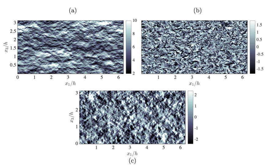
Figure 16: Instantaneous $x_{1}$–$x_{3}$ planes of the (a) streamwise, (b) wall-normal, and (c) spanwise velocity for R2000 at $x_{2}/h=0$. The mean flow is from left to right. The colour bars show velocity normalised in wall units.

The intensities of the three fluctuating velocities at $x_{2}/h=0$ are quantified in figure 17 as a function of the slip length and Reynolds number. Intensities remain fairly constant with $Re_{\tau}$ and change slowly with the slip length. For increasing slip length, the streamwise r.m.s. velocity decreases, whereas the wall-normal r.m.s. velocity increases. The spanwise r.m.s. velocity is roughly constant for the range of slip lengths studied. The trend suggests that the three velocities converge to an isotropic state for increasing slip length, which may be caused by the fact that the Robin boundary condition resembles free slip $\partial u_{i}/\partial x_{2}\approx 0$ in such a limit. Note that the free-slip limit is not of interest in the present work as the flow is unable to support a mean shear.

\psfrag{X}{$l/h$}\psfrag{Y}{$\left.\langle{u_{i}^{\prime}}^{2+}\rangle^{1/2}\right|_{w}$}\includegraphics[width=195.12767pt]{figures/rms_w_lslip.eps}

(a)

\psfrag{X}{$l/h$}\psfrag{Y}{$\left.\langle{u_{i}^{\prime}}^{2+}\rangle^{1/2}\right|_{w}$}\psfrag{X}{$Re_{\tau}$}\psfrag{Y}{$\left.\langle{u_{i}^{\prime}}^{2+}\rangle^{1/2}\right|_{w}$}\includegraphics[width=203.80193pt]{figures/rms_w_Retau.eps}

(b)

Figure 17: Streamwise ($\circ$), wall-normal ($\square$), and spanwise ($\triangle$) root-mean-squared fluctuating velocities at $x_{2}/h=0$ for Robin-bounded cases as a function of (a) slip length and (b) friction Reynolds number.

The sizes of the velocity structures are quantified in figure 18 through the two-point correlation of the velocities as a function of the streamwise and spanwise increments $\delta x_{1}$ and $\delta x_{3}$, respectively. For a constant slip length, the iso-contours of the correlation scale reasonably well using $h$ for $u_{1}$ and $u_{3}$ and $Re_{\tau}>550$. Some dependence on the Reynolds number can be observed for the correlation of the wall-normal velocity, although the scaling with $h$ is still superior than the scaling using wall units (not shown). Increasing the slip length while maintaining $Re_{\tau}$ (dotted-red line in figure 18) shortens the streamwise velocity correlation and enlarges the size of the $u_{2}$ and $u_{3}$ structures.

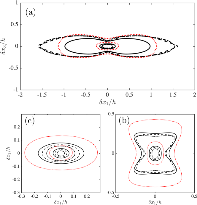
Figure 18: Wall-parallel ($x_{1}-x_{3}$) correlations of the (a) streamwise, (b) wall-normal, and (c) spanwise velocity for R550 (   ), R950 (            ), R2000 (                ), and R550-l1 (            ). Contours are 0.05 and 0.5 of the maximum value. The mean flow is from left to right.

Appendix C Logarithmic layer in Robin-bounded cases with $l$ fixed in wall units

We perform two additional DNSs of Robin-bounded channels with slip length $l^{+}=20$ at $Re_{\tau}\approx 550$ (labelled as R550-lplus) and $Re_{\tau}\approx 950$ (labelled as R950-lplus). The numerical set-up is identical to that discussed in §4.1 for cases R550 and R950. Figure 19(a) shows the diagnostic function $\Xi=x_{2}\partial\langle u_{1}\rangle/\partial x_{2}$ for Robin-bounded cases compared to their no-slip equivalents NS550 and NS950. The agreement between the Robin-bounded and wall-bounded cases is excellent for $x_{2}^{+}\gtrsim 70$. The results are consistent with the adaptation-length argument presented in §4.3: fixing $l$ in wall units introduces a perturbation which propagates in the wall-normal direction for a distance $\mathcal{O}(\nu/u_{\tau})$. While the Reynolds numbers above are too low to develop a well-defined log-layer, the collapse of the diagnostic functions reported in figure 19(a) suggests the emerging of a log-layer for both wall-bounded and Robin-bounded cases. The deviation from the log-layer is further quantified by the error function (see §4.4)

$$\mathcal{E}_{l2}^{+}=\left[\frac{1}{0.2-100/Re_{\tau}}\int_{100/Re_{\tau}}^{0.2}\left(x_{2}^{+}\frac{\partial\langle u_{1}^{+}\rangle}{\partial x_{2}^{+}}-\frac{1}{\kappa}-\frac{x_{2}}{h}\right)^{2}\mathrm{d}(x_{2}/h)\right]^{1/2},$$ (19)

where the lower integration limit is chosen in wall units as expected for the near-wall edge of the log-layer. The results, included in figure 19(b), show that Robin-bounded cases with $l^{+}=20$ tend to a log-layer for $x_{2}/h\in[100/Re_{\tau},0.2]$ with a similar error and at a similar rate as wall-bounded cases. In the cases presented here, the inner-outer scale separation, defined by $h/l$, increases with $Re_{\tau}$. Thus the development of a log-layer may be anticipated by invoking Millikan’s argument.

\psfrag{X}{$x_{2}^{+}$}\psfrag{Y}{$\Xi^{+}$}\includegraphics[width=195.12767pt]{figures/Xi.eps}

(a)

\psfrag{X}{$x_{2}^{+}$}\psfrag{Y}{$\Xi^{+}$}\psfrag{X}{$Re_{\tau}$}\psfrag{Y}{$\mathcal{E}_{l2}^{+}$}\includegraphics[width=195.12767pt]{figures/Umean_convergence_log_20plus.eps}

(b)

Figure 19: (a) Diagnostic function $\Xi=x_{2}\partial\langle u_{1}\rangle/\partial x_{2}$ for NS550 ($\triangledown$), NS950 ($\circ$), R550-lplus (            ), and R950-lplus (            ). (b) $\mathcal{E}_{l2}$ as a function of $Re_{\tau}$ for wall-bounded cases NS550 and NS950 ($\circ$), and Robin-bounded cases R550-lplus and R950-lplus ($\times$).

References

- Abderrahaman-Elena & García-Mayoral (2017) Abderrahaman-Elena, N. & García-Mayoral, R. 2017 Analysis of anisotropically permeable surfaces for turbulent drag reduction. Phys. Rev. Fluids 2, 114609.
- Adrian (2007) Adrian, R. J. 2007 Hairpin vortex organization in wall turbulence. Phys. Fluids 19 (4), 041301.
- Adrian et al. (2000) Adrian, R. J., Meinhart, C. D. & Tomkins, C. D. 2000 Vortex organization in the outer region of the turbulent boundary layer. J. Fluid Mech. 422, 1–54.
- Afzal (1976) Afzal, N. 1976 Millikan’s argument at moderately large Reynolds number. Phys. Fluids 19 (4), 600–602.
- Afzal & Yajnik (1973) Afzal, N. & Yajnik, K. 1973 Analysis of turbulent pipe and channel flows at moderately large reynolds number. J. Fluid Mech. 61 (1), 23–31.
- Agostini & Leschziner (2017) Agostini, L. & Leschziner, M. 2017 Spectral analysis of near-wall turbulence in channel flow at with emphasis on the attached-eddy hypothesis. Phys. Rev. Fluids 2, 014603.
- del Álamo & Jiménez (2003) del Álamo, J. C. & Jiménez, J. 2003 Spectra of the very large anisotropic scales in turbulent channels. Phys. Fluids 15, L41–L44.
- del Álamo & Jiménez (2006) del Álamo, J. C. & Jiménez, J. 2006 Linear energy amplification in turbulent channels. J. Fluid Mech. 559, 205–213.
- del Álamo et al. (2004) del Álamo, J. C., Jiménez, J., Zandonade, P. & Moser, R. D. 2004 Scaling of the energy spectra of turbulent channels. J. Fluid Mech. 500, 135–144.
- Alizard (2015) Alizard, F. 2015 Linear stability of optimal streaks in the log-layer of turbulent channel flows. Phys. Fluids 27 (10), 105103.
- Bae et al. (2018a) Bae, H. J., Lozano-Durán, A., Bose, S. T. & Moin, P. 2018a Dynamic wall model for the slip boundary condition in large-eddy simulation. J. Fluid Mech. pp. 400–432.
- Bae et al. (2018b) Bae, H. J., Lozano-Durán, A., Bose, S. T. & Moin, P. 2018b Turbulence intensities in large-eddy simulation of wall-bounded flows. Phys. Rev. Fluids 3, 014610.
- Bailey et al. (2008) Bailey, S. C. C., Hultmark, M., Smits, A. J. & Schultz, M. P. 2008 Azimuthal structure of turbulence in high Reynolds number pipe flow. J. Fluid Mech. 615, 121–138.
- Bakken et al. (2005) Bakken, O. M., Krogstad, P. Å., Ashrafian, A. & Andersson, H. I. 2005 Reynolds number effects in the outer layer of the turbulent flow in a channel with rough walls. Phys. Fluids 17 (6), 065101.
- Balakumar & Adrian (2007) Balakumar, B. J. & Adrian, R. J. 2007 Large- and very-large-scale motions in channel and boundary-layer flow. Phil. Trans. R. Soc. A 365, 665–681.
- Bullock et al. (1978) Bullock, K. J., Cooper, R. E. & Abernathy, F. H. 1978 Structural similarity in radial correlations and spectra of longitudinal velocity fluctuations in pipe flow. J. Fluid Mech. 88, 585–608.
- Buschmann & Gad-el Hak (2003) Buschmann, M. H. & Gad-el Hak, M. 2003 Generalized logarithmic law and its consequences. AIAA Journal 41 (1), 40–48.
- Chandran et al. (2017) Chandran, D., Baidya, R., Monty, J. P. & Marusic, I. 2017 Two-dimensional energy spectra in high-reynolds-number turbulent boundary layers. J. Fluid Mech. 826, R1.
- Choi et al. (1994) Choi, H., Moin, P. & Kim, J. 1994 Active turbulence control for drag reduction in wall-bounded flows. J. Fluid Mech. 262, 75–110.
- Chung et al. (2014) Chung, D., Monty, J. P. & Ooi, A. 2014 An idealised assessment of townsend’s outer-layer similarity hypothesis for wall turbulence. J. Fluid Mech. 742.
- Coles & Hirst (1969) Coles, D. E. & Hirst, E. 1969 Computation of turbulent boundary layers; 1968 afosr-ifp-stanford conference;.
- Davidson & Krogstad (2009) Davidson, P. A. & Krogstad, P.-A. 2009 A simple model for the streamwise fluctuations in the log-law region of a boundary layer. Phys. Fluids 21 (5), 055105.
- Davidson et al. (2006) Davidson, P. A., Nickels, T. B. & Krogstad, P.-A. 2006 The logarithmic structure function law in wall-layer turbulence. J. Fluid Mech. 550, 51–60.
- De Graaff & Eaton (2000) De Graaff, D. B. & Eaton, J. K. 2000 Reynolds-number scaling of the flat-plate turbulent boundary layer. J. Fluid Mech. 422, 319–346.
- Dong et al. (2017) Dong, S., Lozano-Durán, A., Sekimoto, A. & Jiménez, J. 2017 Coherent structures in statistically stationary homogeneous shear turbulence. J. Fluid Mech. 816, 167–208.
- Flores & Jiménez (2006) Flores, O. & Jiménez, J. 2006 Effect of wall-boundary disturbances on turbulent channel flows. J. Fluid Mech. 566, 357–376.
- Flores & Jiménez (2010) Flores, O. & Jiménez, J. 2010 Hierarchy of minimal flow units in the logarithmic layer. Phys. Fluids 22 (7), 071704.
- Flores et al. (2007) Flores, O., Jiménez, J. & del Álamo, J. C. 2007 Vorticity organization in the outer layer of turbulent channels with disturbed walls. J. Fluid Mech. 591, 145–154.
- Guala et al. (2006) Guala, M., Hommema, S. E. & Adrian, R. J. 2006 Large-scale and very-large-scale motions in turbulent pipe flow. J. Fluid Mech. 554, 521–542.
- Hoyas & Jiménez (2006) Hoyas, S. & Jiménez, J. 2006 Scaling of the velocity fluctuations in turbulent channels up to . Phys. Fluids 18 (1), 011702.
- Hoyas & Jiménez (2008) Hoyas, S. & Jiménez, J. 2008 Reynolds number effects on the Reynolds-stress budgets in turbulent channels. Phys. Fluids 20 (10), 101511.
- Hultmark et al. (2012) Hultmark, M., Vallikivi, M., Bailey, S. C. C. & Smits, A. J. 2012 Turbulent pipe flow at extreme reynolds numbers. Phys. Rev. Lett. 108, 094501.
- Hunt & Morrison (2000) Hunt, J. C. R. & Morrison, J. F. 2000 Eddy structure in turbulent boundary layers. Eur. J. Mech. B Fluids 19, 673–694.
- Hwang & Bengana (2016) Hwang, Y. & Bengana, Y. 2016 Self-sustaining process of minimal attached eddies in turbulent channel flow. J. Fluid Mech. 795, 708––738.
- Hwang & Cossu (2010) Hwang, Y. & Cossu, C. 2010 Self-sustained process at large scales in turbulent channel flow. Phys. Rev. Lett. 105, 044505.
- Jelly et al. (2014) Jelly, T. O., Jung, S. Y. & Zaki, T. A. 2014 Turbulence and skin friction modification in channel flow with streamwise-aligned superhydrophobic surface texture. Phys. Fluids 26 (9), 095102.
- Jiménez (2004) Jiménez, J. 2004 Turbulent flows over rough walls. Annu. Rev. Fluid Mech. 36 (1), 173–196.
- Jiménez (2012) Jiménez, J. 2012 Cascades in wall-bounded turbulence. Annu. Rev. Fluid Mech. 44, 27–45.
- Jiménez (2013) Jiménez, J. 2013 Near-wall turbulence. Phys. Fluids 25 (10), 101302.
- Jiménez (2018) Jiménez, J. 2018 Coherent structures in wall-bounded turbulence. J. Fluid Mech. 842, P1.
- Jiménez & Moin (1991) Jiménez, J. & Moin, P. 1991 The minimal flow unit in near-wall turbulence. J. Fluid Mech. 225, 213–240.
- Jiménez & Moser (2007) Jiménez, J. & Moser, R. D. 2007 What are we learning from simulating wall turbulence? Phil. Trans. R. Soc. A 365 (1852), 715–732.
- Jiménez & Pinelli (1999) Jiménez, J. & Pinelli, A. 1999 The autonomous cycle of near-wall turbulence. J. Fluid Mech. 389, 335–359.
- von Kármán (1930) von Kármán, T. 1930 Mechanische Ahnlichkeit und Turbulenz. In Proceedings Third Int. Congr. Applied Mechanics, Stockholm, pp. 85–105.
- Kim & Moin (1985) Kim, J. & Moin, P. 1985 Application of a fractional-step method to incompressible Navier-Stokes equations. J. Comp. Phys. 59, 308–323.
- Kim & Adrian (1999) Kim, K. & Adrian, R. J. 1999 Very large-scale motion in the outer layer. Phys. Fluids 11 (2), 417–422.
- Lee & Moser (2015) Lee, M. & Moser, R. D. 2015 Direct numerical simulation of turbulent channel flow up to . J. Fluid Mech. 774, 395–415.
- Lee et al. (1990) Lee, M. J., Kim, J. & Moin, P. 1990 Structure of turbulence at high shear rate. J. Fluid Mech. 216, 561–583.
- Lozano-Durán & Bae (2016) Lozano-Durán, A. & Bae, H. J. 2016 Turbulent channel with slip boundaries as a benchmark for subgrid-scale models in LES. Annual Research Briefs, Center for Turbulence Research, Stanford University pp. 97–103.
- Lozano-Durán & Bae (2019) Lozano-Durán, A. & Bae, H. J. 2019 Characteristic scales of Townsend’s wall attached eddies. Annual Research Briefs, Center for Turbulence Research, Stanford University pp. 183–196.
- Lozano-Durán & Borrell (2016) Lozano-Durán, A. & Borrell, G. 2016 Algorithm 964: An efficient algorithm to compute the genus of discrete surfaces and applications to turbulent flows. ACM Trans. Math. Softw. 42 (4), 34:1–34:19.
- Lozano-Durán et al. (2012) Lozano-Durán, A., Flores, O. & Jiménez, J. 2012 The three-dimensional structure of momentum transfer in turbulent channels. J. Fluid Mech. 694, 100–130.
- Lozano-Durán et al. (2018) Lozano-Durán, A., Hack, M. J. P. & Moin, P. 2018 Modeling boundary-layer transition in direct and large-eddy simulations using parabolized stability equations. Phys. Rev. Fluids 3, 023901.
- Lozano-Durán & Jiménez (2014a) Lozano-Durán, A. & Jiménez, J. 2014a Effect of the computational domain on direct simulations of turbulent channels up to . Phys. Fluids 26 (1), 011702.
- Lozano-Durán & Jiménez (2014b) Lozano-Durán, A. & Jiménez, J. 2014b Time-resolved evolution of coherent structures in turbulent channels: characterization of eddies and cascades. J. Fluid Mech. 759, 432–471.
- Luchini (2017) Luchini, P. 2017 Universality of the turbulent velocity profile. Phys. Rev. Lett. 118, 224501.
- Martell et al. (2009) Martell, M. B., Perot, J. B. & Rothstein, J. P. 2009 Direct numerical simulations of turbulent flows over superhydrophobic surfaces. J. Fluid Mech. 620, 31–41.
- Marusic & Monty (2019) Marusic, I. & Monty, J. P. 2019 Attached eddy model of wall turbulence. Annu. Rev. Fluid Mech. 51 (1), null.
- Marusic et al. (2013) Marusic, I., Monty, J. P., Hultmark, M. & Smits, A. J. 2013 On the logarithmic region in wall turbulence. J. Fluid Mech. 716, R3.
- McKeon et al. (2004) McKeon, B. J., Li, J., Jiang, W., Morrison, J. F. & Smits, A. J. 2004 Further observations on the mean velocity distribution in fully developed pipe flow. J. Fluid Mech. 501, 135–147.
- Mellor (1972) Mellor, G. L. 1972 The large reynolds number, asymptotic theory of turbulent boundary layers. Int. J. Eng. Sci. 10 (10), 851–873.
- Meneveau & Marusic (2013) Meneveau, C. & Marusic, I. 2013 Generalized logarithmic law for high-order moments in turbulent boundary layers. J. Fluid Mech. 719, R1.
- Millikan (1938) Millikan, C. B. 1938 A critical discussion of turbulent flows in channels and circular tubes. In Proceedings Int. Congr. Applied Mechanics, New York (ed. J. P. D. Hartog & H. Peters), pp. 386–392. Wiley.
- Min & Kim (2004) Min, T. & Kim, J. 2004 Effects of hydrophobic surface on skin-friction drag. Phys. Fluids 16 (7), L55–L58.
- Mizuno & Jiménez (2011) Mizuno, Y. & Jiménez, J. 2011 Mean velocity and length-scales in the overlap region of wall-bounded turbulent flows. Phys. Fluids 23 (8), 085112.
- Mizuno & Jiménez (2013) Mizuno, Y. & Jiménez, J. 2013 Wall turbulence without walls. J. Fluid Mech. 723, 429–455.
- Moarref et al. (2013) Moarref, R., Sharma, A. S., Tropp, J. A. & McKeon, B. J. 2013 Model-based scaling of the streamwise energy density in high-Reynolds-number turbulent channels. J. Fluid Mech. 734, 275–316.
- Moisy & Jiménez (2004) Moisy, F. & Jiménez, J. 2004 Geometry and clustering of intense structures in isotropic turbulence. J. Fluid Mech. 513, 111–133.
- Monty et al. (2007) Monty, J. P., Stewart, J. A., Williams, R. C. & Chong, M. S. 2007 Large-scale features in turbulent pipe and channel flows. J. Fluid Mech. 589, 147–156.
- Morrison et al. (2004) Morrison, J. F., McKeon, B. J., Jiang, W. & Smits, A. J. 2004 Scaling of the streamwise velocity component in turbulent pipe flow. J. Fluid Mech. 508, 99–131.
- Morrison & Kronauer (1969) Morrison, W. R. B. & Kronauer, R. E. 1969 Structural similarity for fully developed turbulence in smooth tubes. J. Fluid Mech. 39 (1), 117–141.
- Nikuradse (1933) Nikuradse, J. 1933 Laws of flow in rough pipes. VDI Forschungsheft p. 361.
- Oberlack (2001) Oberlack, M. 2001 A unified approach for symmetries in plane parallel turbulent shear flows. J. Fluid Mech. 427, 299–328.
- Orlandi (2000) Orlandi, P. 2000 Fluid Flow Phenomena: A Numerical Toolkit. Springer.
- Park et al. (2013) Park, H., Park, H. & Kim, J. 2013 A numerical study of the effects of superhydrophobic surface on skin-friction drag in turbulent channel flow. Phys. Fluids 25, 0815–.
- Perry & Abell (1975) Perry, A. E. & Abell, C. J. 1975 Scaling laws for pipe-flow turbulence. J. Fluid Mech. 67, 257–271.
- Perry & Abell (1977) Perry, A. E. & Abell, C. J. 1977 Asymptotic similarity of turbulence structures in smooth- and rough-walled pipes. J. Fluid Mech. 79, 785–799.
- Perry & Chong (1982) Perry, A. E. & Chong, M. S. 1982 On the mechanism of wall turbulence. J. Fluid Mech. 119, 173–217.
- Phillips (1987) Phillips, W. R. C. 1987 The wall region of a turbulent boundary layer. Phys. Fluids 30 (8), 2354–2361.
- Prandtl (1925) Prandtl, L. 1925 Bericht über die Entstehung der Turbulenz. Z. Angew. Math. Mech. 5, 136–139.
- Raupach et al. (1991) Raupach, M. R., Antonia, R. A. & Rajagopalan, S. 1991 Rough-wall turbulent boundary layers. Appl. Mech. Rev. 44 (1), 1–25.
- Rosenfeld & Kak (1982) Rosenfeld, A. & Kak, A. C. 1982 Digital Picture Processing: Volume 1 and 2, 2nd edn. Academic Press, Orlando, FL.
- Rotta (1962) Rotta, J. 1962 Turbulent boundary layers in incompressible flow. Prog. Aerosp. Sci. 2 (1), 1 – 95.
- Seo et al. (2015) Seo, J., García-Mayoral, R. & Mani, A. 2015 Pressure fluctuations and interfacial robustness in turbulent flows over superhydrophobic surfaces. J. Fluid Mech. 783, 448–473.
- Seo & Mani (2016) Seo, J. & Mani, A. 2016 On the scaling of the slip velocity in turbulent flows over superhydrophobic surfaces. Phys. Fluids 28 (2), 025110.
- Sillero et al. (2014) Sillero, J. A., Jiménez, J. & Moser, R. D. 2014 Two-point statistics for turbulent boundary layers and channels at Reynolds numbers up to . Phy. Fluids 26 (10), 105109.
- Smits et al. (2011) Smits, A. J., McKeon, B. J. & Marusic, I. 2011 High-Reynolds number wall turbulence. Annu. Rev. Fluid Mech. 43 (1), 353–375.
- Tomkins & Adrian (2003) Tomkins, C. D. & Adrian, R. J. 2003 Spanwise structure and scale growth in turbulent boundary layers. J. Fluid Mech. 490, 37–74.
- Townsend (1961) Townsend, A. A. 1961 Equilibrium layers and wall turbulence. J. Fluid Mech. 11, 97–120.
- Townsend (1976) Townsend, A. A. 1976 The structure of turbulent shear flow. Cambridge University Press.
- Tuerke & Jiménez (2013) Tuerke, F. & Jiménez, J. 2013 Simulations of turbulent channels with prescribed velocity profiles. J. Fluid Mech. 723, 587–603.
- Vallikivi et al. (2015) Vallikivi, M., Ganapathisubramani, B. & Smits, A. J. 2015 Spectral scaling in boundary layers and pipes at very high Reynolds numbers. J. Fluid Mech. 771, 303–326.
- Wosnik et al. (2000) Wosnik, M., Castillo, L. & George, W. K. 2000 A theory for turbulent pipe and channel flows. J. Fluid Mech. 421, 115–145.
- Wray (1990) Wray, A. A. 1990 Minimal-storage time advancement schemes for spectral methods. Tech. Rep. MS 202 A-1. NASA Ames Research Center.
- Zagarola & Smits (1998) Zagarola, M. V. & Smits, A. J. 1998 Mean-flow scaling of turbulent pipe flow. J. Fluid Mech. 373, 33–79.