Quantum steering for continuous variable in de Sitter space

Abstract

We study the distribution of quantum steerability for continuous variables between two causally disconnected open charts in de Sitter space. It is shown that quantum steerability suffers from “sudden death” in de Sitter space, which is quite different from the behaviors of entanglement and discord because the latter always survives and the former vanishes only in the limit of infinite curvature. It is found that the attainment of maximal steerability asymmetry indicates a transition between unidirectional steerable and bidirectional steerable. Unlike in the flat space, the asymmetry of quantum steerability can be completely destroyed in the limit of infinite curvature for the conformal and massless scalar fields in de Sitter space.

I Introduction

Einstein-Podolsky-Rosen steering epr captures the fact that one observer, can nonlocally manipulates, or steers, the state of the other subsystem by performing measurements on one-half of an entangled state. Originally realized by Schrödinger schr ; schr2 , quantum steerability has been understood as a form of intermediate nonlocal correlation between Bell nonlocality and entanglement. It is recognized that steerability is an important resource for quite a few quantum information processing tasks, such as one-sided device-independent quantum key distribution steering1 ; steering11 and subchannel discrimination steering12 . In practice, different from the Bell tests, the demonstration of quantum steerability which is free of detection and locality loopholes is in reach Kocsis , which make quantum steerability a ponderable concept in quantum information theory. For the foregoing reasons, quantum steerability has recently attracted increasing interest both from theoretical wiseman ; Skrzypczyk ; Walborn ; Bowles ; steering2 ; steering3 ; steering4 ; steering5 ; wang2016 ; jieci1 and experimental reid ; Saunders ; Handchen ; Sun ; zeng perspectives. Most recently, Tischler et.al reported an experimental demonstration of unidirectional steering, which is free either of the restrictions on the type of allowed measurements or of assumptions about the quantum state at hand Tischler .

On the other hand, it is of great interest to study the behavior of quantum entanglement and other quantum correlations for discrete variables between causally disconnected regions in the context of cosmology Ball:2005xa ; Fuentes:2010dt ; Nambu:2011ae ; Kanno16 ; wang2015 ; Kanno151 ; Kanno152 ; Kanno153 ; Choudhury . In particular, we know that any two mutually separated regions eventually become causally disconnected in the exponentially expanding de Sitter space. The Bogoliubov transformations between the open chart vacua and the Bunch-Davies vacuum which have support on both regions of a free massive scalar field were derived in Sasaki:1994yt . Later, quantum correlations of scalar fields Maldacena:2012xp ; Albrecht18 ; Kanno:2014lma ; Iizuka:2014rua , Dirac fields Kanno:2016qcc and axion fields  Choudhury:2017bou ; Choudhury2019 were studied in de Sitter space. In Kanno:2014ifa ; Dimitrakopoulos:2015yva , the authors studied the observable effect of quantum information on the cosmic microwave background since there are some entanglement between causally separated regions in de Sitter space. Like entanglement, quantum steerability is one kind of nonlocal quantum correlation which admits no equivalent in classical physics. Therefore, it is important to study the quantum steering between causally disconnected regions of de Sitter space because one can never communicate classically between them.

In this paper we present a quantitative investigation on the distribution of steerability in de Sitter space by employing an operational measure of quantum steerability for continuous variable systems Adesso2015 . We consider the sharing of quantum steerability among three subsystems: subsystems $A$ (observed by Alice) and $B$ (observed by Bob) in region $R$, and subsystem $\bar{B}$ observed by an imaginary observer anti-Bob who is restricted to region $L$ of de Sitter space. We will derive the phase-space description of quantum state evolution for continuous variables basing on the Bogoliubov transformation between the open chart vacua and the Bunch-Davies vacuum. It is found that the quantum steerability between Alice and Bob is apparently affected by the curvature of de Sitter space when the mass parameter $\nu$ approaches to the limit of $\nu=1/2$ (conformal) and $\nu=3/2$ (massless). At the same time, Bob and antiBob can steer each other when the curvature is strong enough even though they are separated by the event horizon, which verifies the nonlocal peculiarity of quantum steerability.

The outline of the paper is as follows. In Sec. II we discuss the dynamics of mode functions and Bogoliubov transformations in de Sitter space. In Sec. III we review the definition and measure of bipartite Gaussian quantum steerability. In Sec. IV we study the distribution of Gaussian quantum steerability in de Sitter space. The last section is devoted to a brief summary.

II Quantization of scalar field in de Sitter space

We consider a free scalar field $\phi$ with mass $m$ initially observed by two experimenters, Alice and Bob, in tthe Bunch-Davies vacuum of de Sitter space. The coordinate frames of open charts in de Sitter space can be obtained by analytic continuation from the Euclidean metric. As shown in Fig. (1), the spacetime geometry of de Sitter space in open charts is divided into three parts denoting by $R$, $L$ and $C$, respectively. We assume that the observer Bob is restricted to region $R$, which is causally disconnected from region $L$. The metrics for the two causally disconnected open charts $R$ and $L$ in the de Sitter space are given by

$$ds^{2}_{R} = H^{-2}\left[-dt^{2}_{R}+\sinh^{2}t_{R}\left(dr^{2}_{R}+\sinh^{2}r_{R}\,d\Omega^{2}\right)\right]\,,$$

$$ds^{2}_{L} = H^{-2}\left[-dt^{2}_{L}+\sinh^{2}t_{L}\left(dr^{2}_{L}+\sinh^{2}r_{L}\,d\Omega^{2}\right)\right]\,,$$ (1)

where $d\Omega^{2}$ is the metric on the two-sphere and $H^{-1}$ is the Hubble radius.

Figure 1: (Color online) The Penrose diagram of the de Sitter space, in which $L$ and $R$ are the two causally disconnected regions described by the open charts.

Solving the Klein-Gordon equation in different regions, one obtains

$$u_{\sigma p\ell m}(t_{R(L)},r_{R(L)},\Omega) \sim \frac{H}{\sinh t_{R(L)}}\,\chi_{p,\sigma}(t_{R(L)})\,Y_{p\ell m}(r_{R(L)},\Omega)\,,\qquad$$

$$-{\rm\bf L^{2}}Y_{p\ell m} = \left(1+p^{2}\right)Y_{p\ell m}\,,$$ (2)

with $Y_{p\ell m}$ being harmonic functions on the three-dimensional hyperbolic space. In Eq. (II) $\chi_{p,\sigma}(t_{R(L)})$ are positive frequency mode functions supporting on the $R$ and $L$ regions  Sasaki:1994yt

$$\chi_{p,\sigma}(t_{R(L)})=\left\{\begin{array}[]{l}\frac{e^{\pi p}-i\sigma e^{-i\pi\nu}}{\Gamma(\nu+ip+\frac{1}{2})}P_{\nu-\frac{1}{2}}^{ip}(\cosh t_{R})-\frac{e^{-\pi p}-i\sigma e^{-i\pi\nu}}{\Gamma(\nu-ip+\frac{1}{2})}P_{\nu-\frac{1}{2}}^{-ip}(\cosh t_{R})\,,\\ \\ \frac{\sigma e^{\pi p}-i\,e^{-i\pi\nu}}{\Gamma(\nu+ip+\frac{1}{2})}P_{\nu-\frac{1}{2}}^{ip}(\cosh t_{L})-\frac{\sigma e^{-\pi p}-i\,e^{-i\pi\nu}}{\Gamma(\nu-ip+\frac{1}{2})}P_{\nu-\frac{1}{2}}^{-ip}(\cosh t_{L})\,,\end{array}\right.$$ (6)

where $P^{\pm ip}_{\nu-\frac{1}{2}}$ are the associated Legendre functions and $\sigma=\pm 1$ distinguishing the independent solutions for each region. These solutions can be normalized by the factor $N_{p}=\frac{4\sinh\pi p\,\sqrt{\cosh\pi p-\sigma\sin\pi\nu}}{\sqrt{\pi}\,|\Gamma(\nu+ip+\frac{1}{2})|}\,.$ In addition, $p$ is a positive real parameter normalized by $H$, and $\nu$ is a mass parameter $\nu=\sqrt{\frac{9}{4}-\frac{m^{2}}{H^{2}}}\,$. Note that the effect of the curvature of the three-dimensional hyperbolic space starts to appear around $p\sim 1$ Kanno16 ; Albrecht18 . In addition, the effect of curvature gets stronger as $p$ becomes smaller than $1$. Therefore, $p$ can be regarded as the curvature parameter of the de Sitter space. It is known that there are two special values for the mass parameter $\nu$: $\nu=1/2$ ($m^{2}=2H^{2}$) for the conformally coupled massless scalar field, and $\nu=3/2$ for the minimally coupled massless limit.

The scalar field can be expanded in terms of the creation and annihilation operators:

$$\hat{\phi}(t,r,\Omega)=\frac{H}{\sinh t}\int dp\sum_{\ell,m}\phi_{p\ell m}(t)Y_{p\ell m}(r,\Omega)\,,$$ (7)

where the Fourier mode field operator $\phi_{p\ell m}(t)\equiv\sum_{\sigma}\left[\,a_{\sigma p\ell m}\,\chi_{p,\sigma}(t)+a_{\sigma p\ell-m}^{\dagger}\,\chi^{*}_{p,\sigma}(t)\right]$ has been introduced, and $a_{\sigma p\ell m}|0\rangle_{\rm BD}=0$ is the annihilation operator of the Bunch-Davies vacuum. For simplicity, hereafter we omit the indices $p$, $\ell$, $m$ of $\phi_{p\ell m}$, $a_{\sigma p\ell m}$ and $a_{\sigma p\ell-m}^{\dagger}$. Similarly, the mode functions and the associated Legendre functions are rewritten in simple forms: $\chi_{p,\sigma}(t)\rightarrow\chi^{\sigma}$, $P_{\nu-1/2}^{ip}(\cosh t_{R,L})\rightarrow P^{R,L}$, and $P_{\nu-1/2}^{-ip}(\cosh t_{R,L})\rightarrow P^{R*,L*}$.

Then we consider the positive frequency mode functions

$$\varphi^{q}=\left\{\begin{array}[]{ll}\tilde{N}_{p}^{-1}P^{q}{}&\mbox{in region}~{}q\,,\\ 0{}&\mbox{in the opposite region}\,,\end{array}\right.\quad\tilde{N}_{p}=\frac{\sqrt{2p}}{|\Gamma(1+ip)|}\,,$$ (10)

for the $R$ or $L$ vacuum which are defined only on the $q=(R,L)$ region, respectively. Since the Fourier mode field operator should be the same under the change of mode functions, we can relate the operators $(a_{\sigma},a_{\sigma}^{\dagger})$ and $(b_{q},b_{q}^{\dagger})$ by a Bogoliubov transformation

$$\phi(t)=a_{\sigma}\,\chi^{\sigma}+a_{\sigma}^{\dagger}\,\chi^{\sigma}{}^{*}=b_{q}\,\varphi^{q}+b_{q}^{\dagger}\,\varphi^{q}{}^{*}\,,$$ (11)

where the creation and annihilation operators ($b_{q},b_{q}^{\dagger}$) in different regions are introduced to ensure $b_{q}|0\rangle_{q}=0$.

Using the Bogoliubov transformation between the operators, the Bunch-Davies vacuum can be constructed from the vacuum states over $|0\rangle_{q}$ in regions $R$ and $L$, which is

$$|0\rangle_{\rm BD}\propto\exp\left(\frac{1}{2}\sum_{i,j=R,L}m_{ij}\,b_{i}^{\dagger}\,b_{j}^{\dagger}\right)|0\rangle_{R}|0\rangle_{L}\,,$$ (12)

where $m_{ij}$ is a symmetric matrix determined by $a_{\sigma}|0\rangle_{\rm BD}=0$:

$$m_{ij}=\frac{\sqrt{2}\,e^{-p\pi}}{\sqrt{\cosh 2\pi p+\cos 2\pi\nu}}\left(\begin{array}[]{cc}\cos\pi\nu&i\sinh p\pi\vspace{1mm}\\ i\sinh p\pi&\cos\pi\nu\\ \end{array}\right)\,.$$ (15)

We can see that the Bunch-Davies vacuum is in fact an entangled two mode squeezed state in the ${\cal H}_{R}\otimes{\cal H}_{L}$ Hilbert space. It is worth noting that the density matrix $\rho=|0\rangle_{\rm BD}\,{}_{\rm BD}\langle 0|$ is diagonal only for $\nu=1/2$ or $3/2$.

To make the calculation easier for tracing out the degrees of freedom in the $L$ space later, a diagonal density matrix like

$$|0\rangle_{\rm BD}=N_{\gamma_{p}}^{-1}\exp\left(\gamma_{p}\,c_{R}^{\dagger}\,c_{L}^{\dagger}\,\right)|0\rangle_{R^{\prime}}|0\rangle_{L^{\prime}}\,,$$ (16)

is required. To this end we introduce new operators $c_{q}=(c_{R},c_{L})$ that satisfy Kanno16 ; Albrecht18

$$c_{R}=u\,b_{R}+v\,b_{R}^{\dagger}\,,\qquad c_{L}=u^{*}\,b_{L}+v^{*}\,b_{L}^{\dagger}\,.$$ (17)

Apparently, this Bogoliubov transformation does not mix the operators in the open chart $R$ and those in open chart $L$. Note that the condition $|u|^{2}-|v|^{2}=1$ is assumed to ensure the commutation relation $[c_{i},(c_{j})^{\dagger}]=\delta_{ij}$. The normalization factor $N_{\gamma_{p}}$ in Eq. (16) is given by

$$N_{\gamma_{p}}^{2}=\left|\exp\left(\gamma_{p}\,c_{R}^{\dagger}\,c_{L}^{\dagger}\,\right)|0\rangle_{R^{\prime}}|0\rangle_{L^{\prime}}\right|^{2}=\frac{1}{1-|\gamma_{p}|^{2}}\,.$$ (18)

Considering the definition of $c_{R}$ and $c_{L}$ in Eq. (17) and the consistency relations from Eq. (16), it is demanded that $c_{R}|0\rangle_{\rm BD}=\gamma_{p}\,c_{L}^{\dagger}|0\rangle_{\rm BD}$, $c_{L}|0\rangle_{\rm BD}=\gamma_{p}\,c_{R}^{\dagger}|0\rangle_{\rm BD}$, which give Kanno16 ; Albrecht18

$$\gamma_{p}=\frac{1}{2\zeta}\left[-\omega^{2}+\zeta^{2}+1-\sqrt{\left(\omega^{2}-\zeta^{2}-1\right)^{2}-4\zeta^{2}}\,\right]\,,$$

where we defined $\omega\equiv m_{RR}=m_{LL}$ and $\zeta\equiv m_{RL}=m_{LR}$ in Eq. (15). Putting the matrix elements of Eq. (15) into Eq. (II), we obtain

$$\gamma_{p}=i\frac{\sqrt{2}}{\sqrt{\cosh 2\pi p+\cos 2\pi\nu}+\sqrt{\cosh 2\pi p+\cos 2\pi\nu+2}}\,.$$ (19)

For the conformally coupled massless scalar ($\nu=1/2$) and the minimally coupled massless scalar ($\nu=3/2$), $\gamma_{p}$ simplifies to $|\gamma_{p}|=e^{-\pi p}$.

III Measurement of quantum steerability for continuous variables

In this section we introduce the definition and measurement of quantum steerability for continuous variables. We consider a bosonic bipartite continuous variable quantum system weedbrook represented by $(n+m)$ modes. The bipartite state consist of two subsystems: the first subsystem is observed by Alice ($A$) with $n$ modes and the second subsystem for Bob ($B$) of $m$ modes. For each mode $i$, the corresponding phase-space operators $\hat{x}_{i}^{A(B)},\,\,\hat{p}_{i}^{A(B)}$ are defined by $\hat{a}_{i}^{A}=\frac{\hat{x}_{i}^{A}+i\hat{p}_{i}^{A}}{\sqrt{2}}$ and $\hat{a}_{i}^{B}=\frac{\hat{x}_{i}^{B}+i\hat{p}_{i}^{B}}{\sqrt{2}}$. These phase-space variables grouped for convenience into the vector $\hat{R}=(\hat{x}_{1}^{A},\hat{p}_{1}^{A},\ldots,\hat{x}_{n}^{A},\hat{p}_{n}^{A},\hat{x}_{1}^{B},\hat{p}_{1}^{B},\ldots,\hat{x}_{m}^{B},\hat{p}_{m}^{B})^{\sf T}$, satisfying the canonical commutation relations $[{{{\hat{R}}_{i}},{{\hat{R}}_{j}}}]=i{\Omega_{ij}}$, with $\Omega=\bigoplus_{1}^{n+m}{{\ 0\ \ 1}\choose{-1\ 0}}$ being the symplectic form. The character of a Gaussian state ${\rho_{AB}}$ is is completely prescribed by its first and second statistical moments. The latter is a covariance matrix with elements ${\sigma_{ij}}=\text{Tr}\big{[}{{{\{{{{\hat{R}}_{i}},{{\hat{R}}_{j}}}\}}_{+}}\ {\rho_{AB}}}\big{]}$ and can always be put into a block form

$$\sigma_{AB}=\left({\begin{array}[]{*{20}{c}}A&C\\ {{C^{\sf T}}}&B\\ \end{array}}\right).$$ (20)

Here the submatrices $A$ and $B$ are the covariance matrixes corresponding to the reduced states of Alice’s and Bob’s subsystems respectively. In addition, a covariance matrix $\sigma_{AB}$ that can describe a physical quantum state if and only if (iff ) the bona fide uncertainty principle relation

$${\sigma_{AB}}+i\,({\Omega_{AB}})\geq 0,$$ (21)

is satisfied.

Now let us give the definition of quantum steerability in continuous variable systems. We consider a pair of local observables $R_{A}$ ( on $A$ with outcome $r_{A}$) and $R_{B}$ (on $B$ with outcome $r_{B}$) in a bipartite state $\rho_{AB}$. After Alice performs a set of measurements $\mathcal{M}_{A}$, the state is steerable iff it is not possible to express the joint probability as wiseman

$$P\left({{r_{A}},{r_{B}}|{R_{A}},{R_{B}},{\rho_{AB}}}\right)=\sum\limits_{\lambda}{{\wp_{\lambda}}}\,\wp\left({{r_{A}}|{R_{A}},\lambda}\right)P\left({{r_{B}}|{R_{B}},{\rho_{\lambda}}}\right),$$ (22)

where ${\wp_{\lambda}}$ and $\wp\left({{r_{A}}|{R_{A}},\lambda}\right)$ are probability distributions, involving the local hidden variable $\lambda$. In addition, $P\left({{r_{B}}|{R_{B}},{\rho_{\lambda}}}\right)$ is the conditional probability distribution associated to the extra condition of being evaluated on the state $\rho_{\lambda}$. Like the Bell nonlocality, quantum steering is exhibited in a state iff the correlations between A and B cannot be explained by a local hidden variable model. In other words, at least one measurement set is required to violate the expression when ${\wp_{\lambda}}$ is fixed across all measurements.

As proposed in wiseman , a Gaussian state $\rho_{AB}$ is $A\to B$ steerable iff the condition

$${\sigma_{AB}}+i\,({0_{A}}\oplus{\Omega_{B}})\geq 0,$$

is violated by Alice’s Gaussian measurements. Employing Eq. (20), we can see that the inequality given in Eq. (91) equals to two simultaneous conditions: (i) $A>0$, and (ii) ${M^{B}_{\sigma}}+i{\Omega_{B}}\geq 0$, with $M^{B}_{\sigma}=B-{C^{\sf T}}{A^{-1}}C$ being the Schur complement of $A$ in the CM $\sigma_{AB}$. Note that the first condition is always verified because $A$ is a physical covariance matrix. Therefore, $\sigma_{AB}$ is $A\to B$ steerable iff the symmetric and positive definite $2m\times 2m$ matrix $M^{B}_{\sigma}$ is not a bona fide covariance matrix wiseman .

According to Williamson’s theorem williamson , the symmetric matrix $M^{B}_{\sigma}$ is diagonalized by a symplectic transformation $S_{B}$ such that $S_{B}M^{B}_{\sigma}S_{B}^{\sf T}=\text{diag}\{\bar{\nu}^{B}_{1},\bar{\nu}^{B}_{1},\ldots,\bar{\nu}^{B}_{m},\bar{\nu}^{B}_{m}\}$, where $\{\bar{\nu}^{B}_{j}\}$ are the symplectic eigenvalues of $M^{B}_{\sigma}$. Then the degree of $A\to B$ steerability can be measured by Adesso2015

$${\cal G}^{A\to B}(\sigma_{AB}):=\max\bigg{\{}0,\,-\sum_{j:\bar{\nu}^{B}_{j}<1}\ln(\bar{\nu}^{B}_{j})\bigg{\}}\,,$$ (23)

which quantifies the amount by which the condition given by Eq. (III) fails to be fulfilled. This is the Gaussian $A\to B$ steerability, which is invariant under local symplectic operations, it vanishes iff the state described by Eq. (20) is nonsteerable by Gaussian measurements. In other words, the $A\to B$ steerability in fact quantifies the degree by which the condition (III) fails to be fulfilled by Alice’s measurement.

If the steered party Bob has one mode only, the $A\to B$ steerability acquires this form Adesso2015

$${\cal G}^{A\to B}(\sigma_{AB})=\max\big{\{}0,\,{\cal S}(\sigma_{A})-{\cal S}(\sigma_{AB})\big{\}}\,,$$ (24)

with ${\cal S}(\sigma)=\frac{1}{2}\ln(\det\sigma)$ being the Rényi-$2$ entropy renyi . Also, the Gaussian $B\to A$ steerability can be defined by swapping the roles of $A$ and $B$ in Eq. (94). In a quantum information scenario, quantum steerability corresponds to the task of quantum information distribution by an untrusted party wiseman . If Alice and Bob share a $A\to B$ steerable state, the untrusted Alice is able to convince Bob that the shared state is entangled by performing local measurements and classical communication wiseman .

IV Distribution of Gaussian quantum steerability in de Sitter space

IV.1 Reduction of quantum steerability between initially correlated modes

We assume that Alice is a global observer who stays at the Bunch-Davies vacuum, while Bob is an open chart observer resides in the R region of the de Sitter space. The initial state of the modes is prepared by an entangled Gaussian two-mode squeezed state in the Bunch-Davies vacuum, which is described by the covariance matrix

$$\sigma^{\rm(G)}_{AB}(s)=\left(\!\!\begin{array}[]{cccc}\cosh(2s)&0&\sinh(2s)&0\\ 0&\cosh(2s)&0&-\sinh(2s)\\ \sinh(2s)&0&\cosh(2s)&0\\ 0&-\sinh(2s)&0&\cosh(2s)\end{array}\!\!\right),$$ (29)

where $s$ is the squeezing of the initial state. The derivation of the covariance matrix for a two-mode squeezed state is given in Appendix A. In Eq. (29), the basic vectors of the covariance matrix are $|ij\rangle=|i\rangle_{A}|j\rangle_{B}$, which denote the state are observer by Alice (A) and Bob (B). Considering there is no initial correlation between the entire state $\sigma^{\rm(G)}_{AB}(s)$ and the subsystem observed by anti-Bob, the initial covariance matrix of the entire system is $\sigma^{\rm(G)}_{AB}(s)\oplus I_{\bar{B}}$.

As showed in Kanno16 , the Bunch-Davies vacuum for a global observer can be expressed as a two-mode squeezed state of the $R$ and $L$ vacua

$$|0\rangle_{\rm BD}=\sqrt{1-|\gamma_{B}|^{2}}\,\sum_{n=0}^{\infty}\gamma_{B}^{n}|n\rangle_{L}|n\rangle_{R}\,,$$

where $\gamma_{B}$ is the squeezing parameter given in Eq. (19). In the Fock space, the two-mode squeezed state can be obtained by $|0\rangle_{\rm BD}=\hat{U}_{R,L}(\gamma_{p})|0\rangle_{R}|0\rangle_{L}$, where $\hat{U}_{R,L}(\gamma_{p})=e^{\gamma_{p}(\hat{c}^{\dagger}_{\text{R}}\hat{c}^{\dagger}_{\text{L}}-\hat{c}_{\text{R}}\hat{c}_{\text{L}})}$ is the two mode squeezing operator. In the phase space, such transformation can be expressed by a symplectic operator

$$S_{B,\bar{B}}(\gamma_{B})=\frac{1}{\sqrt{1-|\gamma_{B}|^{2}}}\left(\!\!\begin{array}[]{cccc}1&0&|\gamma_{B}|&0\\ 0&1&0&-|\gamma_{B}|\\ |\gamma_{B}|&0&1&0\\ 0&-|\gamma_{B}|&0&1\end{array}\!\!\right)$$ (34)

where $|kl\rangle=|k\rangle_{B}|l\rangle_{\bar{B}}$, which denotes that squeezing transformation are performed to the bipartite state shared between Bob and anti-Bob ($\bar{B}$).

Under this transformation, the mode observed by Bob is mapped into two open charts. That is to say, an extra set of modes $\bar{B}$ becomes relevant from the perspective of a observer in the open charts. Therefore, a complete description of the system involves three modes, mode $A$ described by Alice, mode $B$ described by the Bob in the $R$ chart, and mode $\bar{B}$ by a hypothetical observer anti-Bob confined in the $L$ chart. The covariance matrix of the entire state is given by adesso3

$$\sigma_{AB\bar{B}}(s,\gamma_{B}) = \big{[}I_{A}\oplus S_{B,\bar{B}}(\gamma_{B})\big{]}\big{[}\sigma^{\rm(G)}_{AB}(s)\oplus I_{\bar{B}}\big{]}$$ (35)

$$\big{[}I_{A}\oplus S_{B,\bar{B}}(\gamma_{B})\big{]}\,,$$

where $S_{B,\bar{B}}(\gamma_{B})$ is the phase-space representation of the two-mode squeezing transformation given in Eq. (34). For detail please see Appendix B.

Because Bob in chart $R$ have no access to the modes in the causally disconnected $L$ region, we must therefore trace over the inaccessible modes. Taking the trace over mode $\bar{B}$ in chart $L$, one obtains covariance matrix $\sigma_{AB}(s,\gamma_{B})$ for Alice and Bob

$$\sigma_{AB}(s,\gamma_{B})=\left(\!\!\begin{array}[]{cccc}\cosh(2s)&0&\frac{\sinh(2s)}{\sqrt{1-|\gamma_{B}|^{2}}}&0\\ 0&\cosh(2s)&0&-\frac{\sinh(2s)}{\sqrt{1-|\gamma_{B}|^{2}}}\\ \frac{\sinh(2s)}{\sqrt{1-|\gamma_{B}|^{2}}}&0&\frac{|\gamma_{B}|^{2}+\cosh(2s)}{1-|\gamma_{B}|^{2}}&0\\ 0&-\frac{\sinh(2s)}{\sqrt{1-|\gamma_{B}|^{2}}}&0&\frac{|\gamma_{B}|^{2}+\cosh(2s)}{1-|\gamma_{B}|^{2}}\end{array}\!\!\right).$$ (40)

Employing Eq. (92), the $A\to B$ Gaussian steerability is found to be

$${\cal G}^{A\to B}=\mbox{$\max\big{\{}0,\,\ln{\frac{\cosh(2s)(1-|\gamma_{B}|^{2})}{1+|\gamma_{B}|^{2}\cosh(2s)}}\big{\}}$}.$$ (41)

From Eq. (41) we can see that the $A\to B$ Gaussian steerability depends not only the squeezing parameter $s$, but also the curvature parameter $p$ and mass parameter $\nu$ of the de Sitter space. To check if the quantum steerability is symmetric in de Sitter space, we also calculate the steerability ${\cal G}^{B\to A}$

$${\cal G}^{B\to A}=\mbox{$\max\big{\{}0,\,\ln{\frac{\cosh(2s)+|\gamma_{B}|^{2}}{1+|\gamma_{B}|^{2}\cosh(2s)}}\big{\}}$}.$$ (42)

Since the $A\to B$ steering and the $B\to A$ steering are defined in terms of measurements performed by different observers, the quantum steering is asymmetry in general. In this paper the asymmetry between A and B appears because the squeezing transformation only acts between Bob and anti-Bob. As we can see from Eq. (35), the symplectic operator for the entire system is $\big{[}I_{A}\oplus S_{B,\bar{B}}(\gamma_{B})\big{]}$, which leads the asymmetry between Alice and Bob.

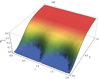
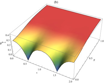
Figure 2: (Color online). The Gaussian quantum steerability ${\cal G}^{A\to B}$ (left) and ${\cal G}^{B\to A}$ (right) as functions of the curvature parameter $p$ and mass parameter $\nu$ of the de Sitter space. The initial squeezing parameter of the two-mode squeezed state is fixed as $s=0.5$.

In Fig. (1) we plot the steerability ${\cal G}^{A\to B}$ (left) and ${\cal G}^{B\to A}$ (right) as functions of the curvature parameter $p$ and mass parameter $\nu$ for a fixed squeezing $s=0.5$. We can see that both the $A\to B$ and $B\to A$ steerability monotonically decrease with the decrease of curvature parameter $p$, which means that space curvature in de Sitter space will destroy the steerability between the initially modes. However, the quantum steerability is apparently affected by the curvature of de Sitter space only around $\nu=1/2$ (conformal scalar limit) and $\nu=3/2$ (massless scalar limit). It is shown that for $\nu=1/2$ (conformal) and $\nu=3/2$ (massless), the $B\to A$ steerability vanishes only in the limit of infinite curvature $p\to 0$. However, the $A\to B$ steerability suffers from “sudden death” when the parameters satisfy $|\gamma_{B}|=\sqrt{\frac{1-sech(2s)}{2}}$, which is quite different from the behavior entanglement and discord in de Sitter space. It was found that quantum discord always survives Kanno16 while entanglement negativity vanishes only in the limit of infinite curvature Maldacena:2012xp ; Albrecht18 ; Kanno:2014lma ; Iizuka:2014rua .

The “sudden death” of quantum steerability indicates the fact that it reduces to zero for finite curvature in de Sitter space, while entanglement vanishes only in the limit of infinite curvature. That is to say, comparing with entanglement, quantum steerability is more sensitive under the influence of space curvature. The physical interpretation of this behavior is very intuitive. It is known that a quantum state with $\eta_{0}\leq\eta<\eta_{e}$ is entangled, where $\eta_{0}=\mu_{A}\mu_{B}+|\mu_{A}-\mu_{B}|$, $\eta_{e}=\sqrt{\mu_{A}^{2}+\mu_{B}^{2}-\mu_{A}^{2}\mu_{B}^{2}}$ and $\mu_{A(B)}=1/\sqrt{\det A(B)}$ Adesso2015 . However, a quantum state which satisfies $\eta\geq\{\mu_{A},\mu_{B}\}$is nonsteerable; a state with $\eta<\mu_{B}$ is $A\to B$ steerable; while a state with $\eta<\mu_{A}$ is $B\to A$ steerable, which are within the entangled region.This again proves the fact that quantum steerability is an intermediate nonlocal correlation between entanglement and Bell nonlocality .

IV.2 Generating quantum steerability between initially uncorrelated modes

To explore the distribution of quantum steerability in de Sitter space, we have to know the behavior of steerability between all the bipartite pairs in the tripartite quantum system. Tracing over the modes in $B$, we obtain the covariance matrix $\sigma_{A\bar{B}}(s,\gamma_{B})$ between the mode observed by Alice in the $R$ region and anti-Bob in $L$ region

$$\sigma_{A\bar{B}}(s,\gamma_{B})=\left(\!\!\begin{array}[]{cccc}\cosh(2s)&0&\frac{|\gamma_{B}|\sinh(2s)}{\sqrt{1-|\gamma_{B}|^{2}}}&0\\ 0&\cosh(2s)&0&\frac{|\gamma_{B}|\sinh(2s)}{\sqrt{1-|\gamma_{B}|^{2}}}\\ \frac{|\gamma_{B}|\sinh(2s)}{\sqrt{1-|\gamma_{B}|^{2}}}&0&\frac{1+|\gamma_{B}|^{2}\cosh(2s)}{1-|\gamma_{B}|^{2}}&0\\ 0&\frac{|\gamma_{B}|\sinh(2s)}{\sqrt{1-|\gamma_{B}|^{2}}}&0&\frac{1+|\gamma_{B}|^{2}\cosh(2s)}{1-|\gamma_{B}|^{2}}\end{array}\!\!\right).$$ (47)

Interestingly, we find the mode described by Alice the mode described by anti-Rob cannot steer each other because ${\cal G}^{A\to\bar{B}}={\cal G}^{\bar{B}\to A}=0$ for any parameters. In fact, this bipartite state is separable under the Peres-Horodecki separability criterion for continuous variable systems Simon .

We also interested in the steerability between mode $B$ in the $R$ region and anti-Bob in $L$ region, which are separated by the event horizon of the de Sitter space. Tracing over the modes in $A$, we obtain the covariance matrix $\sigma_{B\bar{B}}(s,\gamma_{B})$ for Bob and anti-Bob

$$\sigma_{B\bar{B}}(s,\gamma_{B})=\left(\!\!\begin{array}[]{cccc}\frac{|\gamma_{B}|^{2}+\cosh(2s)}{1-|\gamma_{B}|^{2}}&0&\frac{2|\gamma_{B}|\cosh^{2}(s)}{1-|\gamma_{B}|^{2}}&0\\ 0&\frac{|\gamma_{B}|^{2}+\cosh(2s)}{1-|\gamma_{B}|^{2}}&0&-\frac{2|\gamma_{B}|\cosh^{2}(s)}{1-|\gamma_{B}|^{2}}\\ \frac{2|\gamma_{B}|\cosh^{2}(s)}{1-|\gamma_{B}|^{2}}&0&\frac{1+|\gamma_{B}|^{2}\cosh(2s)}{1-|\gamma_{B}|^{2}}&0\\ 0&-\frac{2|\gamma_{B}|\cosh^{2}(s)}{1-|\gamma_{B}|^{2}}&0&\frac{1+|\gamma_{B}|^{2}\cosh(2s)}{1-|\gamma_{B}|^{2}}\end{array}\!\!\right).$$ (52)

Then we calculate the $B\to\bar{B}$ and $\bar{B}\to B$ steerability, which are found to be

$${\cal G}^{B\to\bar{B}}=\mbox{$\max\big{\{}0,\,\ln{\frac{1+sech(2s)|\gamma_{B}|^{2}}{1-|\gamma_{B}|^{2}}}\big{\}}$},$$ (53)

and

$${\cal G}^{\bar{B}\to B}=\mbox{$\max\big{\{}0,\,\ln{\frac{sech(2s)+|\gamma_{B}|^{2}}{1-|\gamma_{B}|^{2}}}\big{\}}$},$$ (54)

respectively.

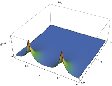
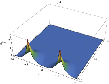
Figure 3: (color online). The Gaussian quantum steerability ${\cal G}^{B\to\bar{B}}$ (left) and ${\cal G}^{\bar{B}\to B}$ (right) as functions of the curvature parameter $p$ and mass parameter $\nu$ of the de Sitter space. The initial squeezing parameter is fixed as $s=0.5$.

In Fig. (3) we plot the Gaussian quantum steerability between Bob and anti-Bob as functions of $p$ and $\nu$ with fixed squeezing $s=0.5$. It is shown that quantum steerability are generated between Bob and Anti-Bob when the curvature parameter $p$ is very small and the mass parameter are around $\nu=1/2$ and $\nu=3/2$ . We find that both the ${\cal G}^{B\to\bar{B}}$ and ${\cal G}^{\bar{B}\to B}$ steerability are generated when the curvature becomes stronger and stronger. That is to say, Bob and antiBob can steer each other when the curvature is strong enough even though they are separated by the event horizon, which verifies the fact that the quantum steerability is one kind of nonlocal quantum correlation.

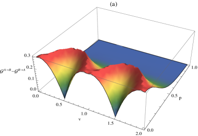
Figure 4: (color online). The Gaussian steerability asymmetry between A and B (left), as well as the asymmetry between B and $\bar{B}$ (right) as functions of the curvature parameter $p$ and mass parameter $\nu$ of the de Sitter space. The initial squeezing parameter is fixed as $s=0.5$.

To check the degree of steerability asymmetric in de Sitter space, we compute the Gaussian steerability asymmetry $|{\cal G}^{A\to B}-{\cal G}^{B\to A}|$ and $|{\cal G}^{B\to\bar{B}}-{\cal G}^{\bar{B}\to B}|$. In Fig. (4) we plot the Gaussian steerability asymmetry between Alice and Bob, as well as the asymmetry between Bob and anti-Bob as functions of the curvature and mass parameters. As shown in Fig. (4a), the steerability asymmetry between Alice and Bob increases with decreasing curvature parameter $p$, which demonstrates that the space curvature destroys the symmetry of initial steerability. It is shown that the condition which sets maximizing the steerability asymmetry between Alice and Bob is $|\gamma_{B}|=\sqrt{\frac{1-sech(2s)}{2}}$, which is exactly the “sudden death” condition of $A\to B$ steerability in Fig. (2). That is, the steerability asymmetry takes the maximum value when the state is un-steerable in the $A\to B$ direction. The attaining of the peak of steerability asymmetry indicates the system experiences a transformation from bidirectional steerability to unidirectional steerability.

In Fig. (4b) we can see that the maximum steerability asymmetry between Bob and anti-Bob is also attained at $|\gamma_{B}|=\sqrt{\frac{1-sech(2s)}{2}}$, which is identical with the condition of the $A-B$ steering asymmetry. Different from the Alice-Bob asymmetry, the attainment of maximal steerability asymmetry between Bob and anti-Bob indicates the transition from unidirectional steerability to bidirectional steerability in the de Sitter space. It is interesting to note that, like the $A-B$ steerability asymmetry, the steerability asymmetry disappear in the limit of infinite curvature $p\to 0$ for $\nu=1/2$ (conformal) and $\nu=3/2$ (massless). However, the steerability asymmetry disappears because both the $A\to B$ and $B\to A$ steerability equal to zero in this limit. Differently, the $B-\bar{B}$ steerability is symmetry when both the $B\to\bar{B}$ and $\bar{B}\to B$ steerability take their maximum values. This phenomenon is nontrivial because the quantum steerability is usually asymmetry in the flat spacetime Adesso2015 . We know that the quantum steering is asymmetry in the flat space because the parameters $\mu_{A}$ and $\mu_{B}$ are usually different from each other. This may indicates that the subsystem $B$ and $\bar{B}$ is symmetry in the conformal scalar and massless scalar limit, which deserves further study.

V Conclusions

We have studied the distribution of steerability among the mode $A(B)$ described by Alice (Bob) in the de Sitter region $R$, and the complimentary mode $\bar{B}$ described by a hypothetical observer anti-Bob in the causally disconnected region $L$. We first derive the Bogoliubov transformation between the Euclidean vacuum and the open chart vacua and then obtain a phase-space description of quantum state evolution for continuous variables. We find that the quantum steerability is apparently affected by the curvature of de Sitter space for $\nu=1/2$ (conformal) and $\nu=3/2$ (massless). It is shown that the $A\to B$ steerability suffers from “sudden death”, which is quite different from the behaviors of entanglement and discord because the latter always survives while the former vanishes only in the limit of infinite curvature Kanno16 . In de Sitter space, Bob and antiBob can steer each other when the curvature is strong enough even though they are separated by the event horizon. To verify the asymmetric property of steerability in de Sitter space, we compare the $A-B$ and $B-\bar{B}$ steerability asymmetry. In addition, the maximum asymmetry are obtained when the $A\to B$ steerability experiences “sudden death”. That is to say, the attainment of maximal steerability asymmetry indicates a transition between unidirectional steerable and bidirectional steerable in de Sitter space. Unlike the flat space, the asymmetry of quantum steerability can be completely destroyed in the limit of infinite curvature for some special scalar fields.

Appendix A Covariance Matrix of a Two-Mode Squeezed State in phase space

In this appendix, we compute the covariance matrix of a two-mode squeezed quantum state in phase space. Firstly we introduce the quantities $\hat{x}_{\bm{i}}$ and $\hat{p}_{\bm{i}}$ such that

$$\hat{x}_{\bm{i}}^{B(\bar{B})} = \frac{1}{\sqrt{2}}\left(\hat{a}_{\bm{i}}^{B(\bar{B})}+\hat{a}_{\bm{i}}^{{B(\bar{B})}\dagger}\right)$$ (55)

$$\hat{p}_{\bm{i}}^{B(\bar{B})} = -\frac{i}{\sqrt{2}}\left(\hat{a}_{\bm{i}}^{B(\bar{B})}-\hat{a}_{\bm{i}}^{{B(\bar{B})}\dagger}\right).$$ (56)

Let us now introduce the characteristic function. It is a real function defined on a four-dimensional real space, given by

$$\chi(\xi)=Tr\left[\hat{\rho}\hat{{\cal W}}(\xi)\right],$$ (57)

where $\hat{\rho}$ is obviously the density operator and $\hat{{\cal W}}(\xi)$ is the Weyl operator, namely $\hat{{\cal W}}(\xi)={\rm e}^{i\xi^{\rm T}\hat{R}}$, with $\hat{R}=\left(\hat{x}_{\bm{i}}^{B},\hat{p}^{B}_{\bm{i}},\hat{x}^{\bar{B}}_{-{\bm{i}}},\hat{p}^{\bar{B}}_{-{\bm{i}}}\right)^{\rm T}\equiv\left(\hat{R}_{1},\hat{R}_{2},\hat{R}_{3},\hat{R}_{4}\right)^{\rm T}$.

As a Gaussian state, the two-mode squeezed state has a Gaussian characteristic function given by $\chi(\xi)={\rm e}^{-\xi^{\rm T}\gamma\xi/4},$ where $\gamma$ is the covariance matrix, related to the two-point correlation functions by $\langle\hat{R}_{j}\hat{R}_{k}\rangle=\gamma_{jk}/2+iJ_{jk}/2$. Here, $J$ is the commutator matrix, $iJ_{j,k}=[\hat{R}_{j},\hat{R}_{k}]$, given by $J=J_{1}\oplus J_{1}$ with $J_{1}=\begin{pmatrix}0&1\\ -1&0\end{pmatrix}.$ For a two-mode Gaussian state, the characteristic function $\chi(\xi)$ (where the components of $\xi$ are denoted as $\xi_{1}$, $\xi_{2}$, $\xi_{3}$ and $\xi_{4}$) can be written as Martin16

$$\chi(\xi) = Tr\left[\hat{S}(\gamma_{p})|0^{A}_{\bm{i}},0^{B}_{-{\bm{i}}}\rangle\langle 0^{A}_{\bm{i}},0^{B}_{-{\bm{i}}}|\hat{S}^{\dagger}(\gamma_{p}){\rm e}^{i\xi_{1}\hat{R}_{1}+i\xi_{2}\hat{R}_{2}+i\xi_{3}\hat{R}_{3}+i\xi_{4}\hat{R}_{4}}\right]$$ (58)

$$= Tr\left[|0^{A}_{\bm{i}},0^{B}_{-{\bm{i}}}\rangle\langle 0^{A}_{\bm{i}},0^{B}_{-{\bm{i}}}|\hat{S}^{\dagger}(\gamma_{p}){\rm e}^{i\xi_{1}\hat{R}_{1}+i\xi_{2}\hat{R}_{2}+i\xi_{3}\hat{R}_{3}+i\xi_{4}\hat{R}_{4}}\hat{S}(\gamma_{p})\right]$$ (59)

$$= \sum_{n=0}^{\infty}\sum_{n^{\prime}=0}^{\infty}\langle n_{\bm{i}},n^{\prime}_{-{\bm{i}}}|0^{A}_{\bm{i}},0^{B}_{-{\bm{i}}}\rangle\langle 0^{A}_{\bm{i}},0^{B}_{-{\bm{i}}}|\hat{S}^{\dagger}(\gamma_{p}){\rm e}^{i\xi_{1}\hat{R}_{1}+i\xi_{2}\hat{R}_{2}+i\xi_{3}\hat{R}_{3}+i\xi_{4}\hat{R}_{4}}\hat{S}(\gamma_{p})|n_{\bm{i}},n^{\prime}_{-{\bm{i}}}\rangle$$ (60)

$$= \langle 0^{A}_{\bm{i}},0^{B}_{-{\bm{i}}}|\hat{S}^{\dagger}(\gamma_{p}){\rm e}^{i\xi_{1}\hat{R}_{1}+i\xi_{2}\hat{R}_{2}+i\xi_{3}\hat{R}_{3}+i\xi_{4}\hat{R}_{4}}\hat{S}(\gamma_{p})\hat{R}(\theta_{k})|0^{A}_{\bm{i}},0^{B}_{-{\bm{i}}}\rangle$$ (61)

$$= \langle 0^{A}_{\bm{i}},0^{B}_{-{\bm{i}}}|\hat{S}^{\dagger}(\gamma_{p}){\rm e}^{i\xi_{1}\hat{R}_{1}+i\xi_{2}\hat{R}_{2}}{\rm e}^{+i\xi_{3}\hat{R}_{3}+i\xi_{4}\hat{R}_{4}}\hat{S}(\gamma_{p})|0^{A}_{\bm{i}},0^{B}_{-{\bm{i}}}\rangle$$ (62)

$$= {\rm e}^{i\xi_{1}\xi_{2}/2+i\xi_{3}\xi_{4}/2}\langle 0^{A}_{\bm{i}},0^{B}_{-{\bm{i}}}|\hat{S}^{\dagger}(\gamma_{p}){\rm e}^{i\xi_{1}\hat{R}_{1}}{\rm e}^{i\xi_{2}\hat{R}_{2}}{\rm e}^{i\xi_{3}\hat{R}_{3}}{\rm e}^{i\xi_{4}\hat{R}_{4}}\hat{S}(\gamma_{p})|0^{A}_{\bm{i}},0^{B}_{-{\bm{i}}}\rangle,$$ (63)

where the Baker-Campbell-Hausdorff formula ${\rm e}^{\hat{A}+\hat{B}}={\rm e}^{-[\hat{A},\hat{B}]/2}{\rm e}^{\hat{A}}{\rm e}^{\hat{B}}$ have been used, which is valid if the operators $\hat{A}$ and $\hat{B}$ commute with $[\hat{A},\hat{B}]$. The next step is introducing the operator $\hat{S}\hat{R}(\hat{S}\hat{R})^{\dagger}$ between the exponential factors. To this end we calculate Martin16

$$\hat{S}^{\dagger}(\gamma_{p}){\rm e}^{i\xi_{1}\hat{R}_{1}}\hat{S}(\gamma_{p}) = \hat{S}^{\dagger}(\gamma_{p})\sum_{n=0}^{\infty}\frac{1}{n!}i^{n}\xi_{1}^{n}\hat{R}_{1}^{n}\hat{S}(\gamma_{p})$$ (64)

$$= \sum_{n=0}^{\infty}\frac{1}{n!}i^{n}\xi_{1}^{n}\hat{S}^{\dagger}(\gamma_{p})\hat{R}_{1}^{n}\hat{S}(\gamma_{p}).$$ (65)

By using the fact that

$$\hat{S}^{\dagger}\hat{R}_{1}^{n}\hat{S}=\hat{S}^{\dagger}\hat{R}_{1}\hat{S}\hat{S}^{\dagger}\hat{R}_{1}^{n-1}\hat{S}=\hat{S}^{\dagger}\hat{R}_{1}\hat{S}\hat{S}^{\dagger}\hat{R}_{1}\hat{S}\hat{S}^{\dagger}\hat{R}_{1}^{n-2}\hat{S}=\left(\hat{S}^{\dagger}\hat{R}_{1}\hat{S}\right)^{n},$$ (66)

one can rewrite the series as Martin16

$$\hat{S}^{\dagger}(\gamma_{p}){\rm e}^{i\xi_{1}\hat{R}_{1}}\hat{S}(\gamma_{p}) = \sum_{n=0}^{\infty}\frac{1}{n!}i^{n}\xi_{1}^{n}\left[\hat{S}^{\dagger}(\gamma_{p})\hat{R}_{1}\hat{S}(\gamma_{p})\right]^{n}$$ (67)

$$= {\rm e}^{i\xi_{1}\hat{S}^{\dagger}(\gamma_{p})\hat{R}_{1}\hat{S}(\gamma_{p})}.$$ (68)

Using this result for the four terms of the characteristic function, we arrive at

$$\chi(\xi) = {\rm e}^{i\xi_{1}\xi_{2}/2+i\xi_{3}\xi_{4}/2}\langle 0^{A}_{\bm{i}},0^{B}_{-{\bm{i}}}|{\rm e}^{i\xi_{1}\hat{S}^{\dagger}\hat{R}_{1}\hat{S}}{\rm e}^{i\xi_{2}\hat{S}^{\dagger}\hat{R}_{2}\hat{S}}{\rm e}^{i\xi_{3}\hat{S}^{\dagger}\hat{R}_{3}\hat{S}}{\rm e}^{i\xi_{4}\hat{S}^{\dagger}\hat{R}_{4}\hat{S}}|0^{A}_{\bm{i}},0^{B}_{-{\bm{i}}}\rangle.$$ (69)

To proceed, one has to evaluate the four terms $\hat{S}^{\dagger}\hat{R}_{i}\hat{S}$, which are Martin16

$$\hat{\Omega}_{1} \equiv \hat{S}^{\dagger}(\gamma_{p})\hat{R}_{1}\hat{S}(\gamma_{p})=(\hat{R}_{1}-\hat{R}_{2})\cosh\gamma_{p}+(\hat{R}_{3}+\hat{R}_{4})\sinh\gamma_{p},$$ (70)

$$\hat{\Omega}_{2} \equiv \hat{S}^{\dagger}(\gamma_{p})\hat{R}_{2}\hat{S}(\gamma_{p})=(\hat{R}_{1}+\hat{R}_{2})\cosh\gamma_{p}+(\hat{R}_{3}-\hat{R}_{4})\sinh\gamma_{p},$$ (71)

$$\hat{\Omega}_{3} \equiv \hat{S}^{\dagger}(\gamma_{p})\hat{R}_{3}\hat{S}(\gamma_{p})=(\hat{R}_{1}+\hat{R}_{2})\sinh\gamma_{p}+(\hat{R}_{3}-\hat{R}_{4})\cosh\gamma_{p},$$ (72)

$$\hat{\Omega}_{4} \equiv \hat{S}^{\dagger}(\gamma_{p})\hat{R}_{4}\hat{S}(\gamma_{p})=(\hat{R}_{1}-\hat{R}_{2})\sinh\gamma_{p}+(\hat{R}_{3}+\hat{R}_{4})\cosh\gamma_{p}.$$ (73)

Then we find that the characteristic function takes the form Martin16

$$\chi(\xi) = {\rm e}^{i\xi_{1}\xi_{2}/2+i\xi_{3}\xi_{4}/2}\langle 0^{B}_{\bm{i}},0^{\bar{B}}_{-{\bm{i}}}|{\rm e}^{-i\xi_{1}\xi_{2}/2}{\rm e}^{i\xi_{1}\hat{\Omega}_{1}+i\xi_{2}\hat{\Omega}_{2}}{\rm e}^{-i\xi_{3}\xi_{4}/2}{\rm e}^{i\xi_{3}\hat{\Omega}_{3}+i\xi_{4}\hat{\Omega}_{4}}|0^{B}_{\bm{i}},0^{\bar{B}}_{-{\bm{i}}}\rangle$$ (74)

$$= \langle 0^{B}_{\bm{i}},0^{\bar{B}}_{-{\bm{i}}}|{\rm e}^{i\xi_{1}\hat{\Omega}_{1}+i\xi_{2}\hat{\Omega}_{2}+i\xi_{3}\hat{\Omega}_{3}+i\xi_{4}\hat{\Omega}_{4}}|0^{B}_{\bm{i}},0^{\bar{B}}_{-{\bm{i}}}\rangle$$ (75)

$$= \langle 0^{B}_{\bm{i}},0^{\bar{B}}_{-{\bm{i}}}|{\rm e}^{i\eta_{1}\hat{R}_{1}+i\eta_{2}\hat{R}_{2}+i\eta_{3}\hat{R}_{3}+i\eta_{4}\hat{R}_{4}}|0^{B}_{\bm{i}},0^{\bar{B}}_{-{\bm{i}}}\rangle$$ (76)

$$\equiv \chi_{\rm vac}(\eta_{1},\eta_{2},\eta_{3},\eta_{4}),$$ (77)

where the coefficients $\eta_{i}$ can be expressed as

$$\eta_{1} = \xi_{1}\cosh\gamma_{p}+(\xi_{2}+\xi_{3}+\xi_{4})\sinh\gamma_{p},$$ (78)

$$\eta_{2} = (-\xi_{1}+\xi_{2})\cosh\gamma_{p}+(\xi_{3}-\xi_{4})\sinh\gamma_{p},$$ (79)

$$\eta_{3} = (\xi_{1}+\xi_{2})\sinh\gamma_{p}+(\xi_{3}+\xi_{4})\cosh\gamma_{p},$$ (80)

$$\eta_{4} = (\xi_{1}-\xi_{2})\sinh\gamma_{p}+(-\xi_{3}+\xi_{4})\cosh\gamma_{p}.$$ (81)

Since the definition of the covariance matrix $\gamma$ is given by the expression Martin16

$$\chi(\xi_{1},\xi_{2},\xi_{3},\xi_{4})={\rm e}^{-\xi^{\rm T}\gamma\xi/4}.$$ (82)

It implies that

$$\sum_{i=1}^{4}\eta_{i}^{2}=\sum_{i=1}^{4}\sum_{j=1}^{4}\gamma_{ij}\xi_{i}\xi_{j},$$ (83)

which allows us to infer the components of the covariance matrix.

Using the above expressions of the correlation matrixes, the explicit form of the two-point correlators are obtained by some lengthy but straightforward calculations, which are

$$\langle\hat{x}^{B}_{\bm{i}}\hat{x}^{B}_{\bm{i}}\rangle = \langle\hat{x}^{\bar{B}}_{-{\bm{i}}}\hat{x}^{\bar{B}}_{-{\bm{i}}}\rangle=\cosh(2\gamma_{p}),\quad\langle\hat{p}^{B}_{\bm{i}}\hat{p}^{B}_{\bm{i}}\rangle=\langle\hat{p}^{\bar{B}}_{-{\bm{i}}}\hat{p}^{\bar{B}}_{-{\bm{i}}}\rangle=cosh(2\gamma_{p})$$ (84)

$$\langle\hat{x}^{B}_{\bm{i}}\hat{x}^{\bar{B}}_{-{\bm{i}}}\rangle = \frac{1}{2}\sinh(2\gamma_{p}),\quad\langle\hat{p}^{B}_{\bm{i}}\hat{p}^{\bar{B}}_{-{\bm{i}}}\rangle=-\frac{1}{2}\sinh(2\gamma_{p}),$$ (85)

$$\langle\hat{x}^{B}_{\bm{i}}\hat{p}^{\bar{B}}_{-{\bm{i}}}\rangle = \langle\hat{p}^{B}_{\bm{i}}\hat{x}^{\bar{B}}_{-{\bm{i}}}\rangle=\frac{1}{2}\sinh(2\gamma_{p}),\quad.$$ (86)

Then one obtains the following covariance matrix

$$\sigma_{B\bar{B}}(\gamma_{B})=\begin{pmatrix}\cosh\left(2\gamma_{p}\right)&0&\sinh\left(2\gamma_{p}\right)&\sinh\left(2\gamma_{p}\right)\\ 0&\cosh\left(2\gamma_{p}\right)&\sinh\left(2\gamma_{p}\right)&-\sinh\left(2\gamma_{p}\right)\\ \sinh\left(2\gamma_{p}\right)&\sinh\left(2\gamma_{p}\right)&\cosh\left(2\gamma_{p}\right)&0\\ \sinh\left(2\gamma_{p}\right)&-\sinh\left(2\gamma_{p}\right)&0&\cosh\left(2\gamma_{p}\right)\end{pmatrix},$$ (87)

where $\cosh\gamma_{B}=(\sqrt{1-|\gamma_{B}|^{2}})^{-1}$.

Appendix B The definition and measurement of quantum steerability

In this appendix we introduce the conception and definition of quantum steerability. Under a set of measurements $\mathcal{M}_{A}$ on Alice, a bipartite system is $A\to B$ steerable—i.e., Alice can steer Bob—iff it is not possible for every pair of local observables $R_{A}\in\mathcal{M}_{A}$ on $A$ and $R_{B}$ on $B$ (with respective outcomes $r_{A}$ and $r_{B}$), to express the joint probability as wiseman

$$P\left({{r_{A}},{r_{B}}|{R_{A}},{R_{B}},{\rho_{AB}}}\right)=\sum\limits_{\lambda}{{\wp_{\lambda}}}\,\wp\left({{r_{A}}|{R_{A}},\lambda}\right)P\left({{r_{B}}|{R_{B}},{\rho_{\lambda}}}\right),$$ (88)

where ${\wp_{\lambda}}$ and $\wp\left({{r_{A}}|{R_{A}},\lambda}\right)$ are probability distributions, involving the local hidden variable $\lambda$. In addition, $P\left({{r_{B}}|{R_{B}},{\rho_{\lambda}}}\right)$ is the conditional probability distribution associated to the extra condition of being evaluated on the state $\rho_{\lambda}$. That is, at least one measurement pair $R_{A}$ and $R_{B}$ must violate the expression in Eq. (C1) when ${\wp_{\lambda}}$ is fixed across all measurements. The probability distribution $P\left({{r_{B}}|{R_{B}},{\rho_{\lambda}}}\right)$ means that a complete knowledge of Bob’s devices (but not of Alice’s ones) is required to formulate the steering condition wiseman .

Here we consider the fully Gaussian scenario, where the initial state is a Gaussian state and the observers’ measurement sets $\mathcal{M}_{A,B}$ are also Gaussian (i.e., mapping Gaussian states into Gaussian states). A Gaussian measurement can be described by a positive Gaussian operator with covariance matrix $T^{{R_{A}}}$, satisfying

$${T^{{R_{A}}}}+i\,{\Omega_{A}}\geq 0.$$ (89)

Once Alice makes a measurement $R_{A}$ and gets an outcome $r_{A}$, Bob’s conditioned state $\rho_{B}^{r_{A}|R_{A}}$ is Gaussian. The covariance matrix of Bob after Alice’s measurement is given by wiseman

$$B^{{R_{A}}}=B-C{\left({{T^{{R_{A}}}}+A}\right)^{-1}}{C^{\sf T}},$$ (90)

which is independent of Alice’s outcome.

As has been shown in wiseman , a Gaussian state $\rho_{AB}$ is $A\to B$ steerable by Alice’s Gaussian measurements iff the condition

$${\sigma_{AB}}+i\,({0_{A}}\oplus{\Omega_{B}})\geq 0,$$ (91)

is violated. Henceforth, a violation of Eq. (91) is necessary and sufficient for Gaussian $A\to B$ steerability. Writing this in matrix form, using the covariance matrix in Eq. (20) of the main manuscript, the nonsteerability inequality Eq. (91) is equivalent to two simultaneous conditions: (i) $A>0$, and (ii) ${M^{B}_{\sigma}}+i{\Omega_{B}}\geq 0$, where $M^{B}_{\sigma}=B-{C^{\sf T}}{A^{-1}}C$ is the Schur complement of $A$ in the covariance matrix $\sigma_{AB}$ wiseman . Condition (i) is always verified for any physical covariance matrix. Therefore, $\sigma_{AB}$ is $A\to B$ steerable iff the symmetric matrix $M^{B}_{\sigma}$ is not a bona fide covariance matrix, i.e., if condition (ii) is violated wiseman . According to Williamson’s theorem williamson , the symmetric matrix $M^{B}_{\sigma}$ is diagonalized by a symplectic transformation $S_{B}$ such that $S_{B}M^{B}_{\sigma}S_{B}^{\sf T}=\text{diag}\{\bar{\nu}^{B}_{1},\bar{\nu}^{B}_{1},\ldots,\bar{\nu}^{B}_{m},\bar{\nu}^{B}_{m}\}$, where $\{\bar{\nu}^{B}_{j}\}$ are the symplectic eigenvalues of $M^{B}_{\sigma}$. Then the degree of $A\to B$ steerability can be measured by Adesso2015

$${\cal G}^{A\to B}(\sigma_{AB}):=\max\bigg{\{}0,\,-\sum_{j:\bar{\nu}^{B}_{j}<1}\ln(\bar{\nu}^{B}_{j})\bigg{\}}\,,$$ (92)

which quantifies the amount by which the condition given by Eq. (91) fails to be fulfilled. This is the Gaussian $A\to B$ steerability, which is invariant under local symplectic operations, it vanishes iff the state described by Eq. (20) of the main manuscript is nonsteerable by Gaussian measurements. In other words, the $A\to B$ steerability in fact quantifies the degree by which the condition (91) fails to be fulfilled by Alice’s measurement.

Clearly, the Gaussian $B\to A$ steering can also be obtained by swapping the roles of $A$ and $B$, resulting in an expression like Eq. (92), in which the symplectic eigenvalues of the Schur complement of $B$, $M^{A}_{\sigma}=A-{C}{B^{-1}}{C^{\sf T}}$, appear instead. When the steered party has one mode only, $M^{B}_{\sigma}$ has a single symplectic eigenvalue

$$\bar{\nu}^{B}=\sqrt{\det M^{B}_{\sigma}}.$$ (93)

By defining the Schur complement $\det{\sigma_{AB}}=\det{A}\det{M^{B}_{\sigma}}$, one can obtain that

$${\cal G}^{A\to B}(\sigma_{AB})=\mbox{$\max\big{\{}0,\,\frac{1}{2}\ln{\frac{\det A}{\det\sigma_{AB}}}\big{\}}$}=\max\big{\{}0,\,{\cal S}(A)-{\cal S}(\sigma_{AB})\big{\}}\,,$$ (94)

which is Eq. (14) of the main manuscript. To compute the quantum steering we only need to get the interplay between the global purity $\mu=1/\sqrt{\det\sigma_{AB}}$ and the one-side purities $\mu_{A(B)}=1/\sqrt{\det A(B)}$. Employing the ratio $\eta=(\mu_{A}\mu_{B})/\mu$, one finds that all physical two-mode Gaussian states live in the region $\eta_{0}\leq\eta\leq 1$ where $\eta_{0}=\mu_{A}\mu_{B}+|\mu_{A}-\mu_{B}|$ Adesso2015 . States with $\eta_{s}\leq\eta\leq 1$ where $\eta_{s}=\mu_{A}+\mu_{B}-\mu_{A}\mu_{B}$ are necessarily separable, states with $\eta_{0}\leq\eta<\eta_{e}$ are entangled Adesso2015 , where $\eta_{e}=\sqrt{\mu_{A}^{2}+\mu_{B}^{2}-\mu_{A}^{2}\mu_{B}^{2}}$. Within the entangled region, states which satisfy $\eta\geq\{\mu_{A},\mu_{B}\}$ are nonsteerable; states with $\eta<\mu_{B}$ are $A\to B$ steerable; states with $\eta<\mu_{A}$ are $B\to A$ steerable. For this reason we can see that the quantum steering is asymmetry in the flat space because $\mu_{A}$ and $\mu_{B}$ are usually different from each other. In fact, the asymmetry of steering for Gaussian states in flat space has been experimentally demonstrated in Handchen .

Appendix C Covariance matrix for the final state of the entire system

The final state given in Eq. (19) of the main manuscript is the phase space description of the tripartite system after the curvature-induced squeezing transformation. The covariance matrix for the final state of the entire system is wang20

$$\sigma_{AB\bar{B}}(s,r) = \big{[}I_{A}\oplus S_{B,\bar{B}}(\gamma_{p})\big{]}\big{[}\sigma^{\rm(M)}_{AB}(s)\oplus I_{\bar{B}}\big{]}$$ (98)

$$\big{[}I_{A}\oplus S_{B,\bar{B}}(\gamma_{p})\big{]}$$

$$= \left(\begin{array}[]{ccc}\mathcal{\sigma}_{A}&\mathcal{E}_{AB}&\mathcal{E}_{A\bar{B}}\\ \mathcal{E}^{\sf T}_{AB}&\mathcal{\sigma}_{B}&\mathcal{E}_{B\bar{B}}\\ \mathcal{E}^{\sf T}_{A\bar{B}}&\mathcal{E}^{\sf T}_{B\bar{B}}&\mathcal{\sigma}_{\bar{B}}\\ \end{array}\right)\,,$$

where $\sigma^{\rm(G)}_{AB}(s)\oplus I_{\bar{B}}$ is the initial state of the entire system. In Eq. (C1) the diagonal elements have the following forms: $\mathcal{\sigma}_{A}=\cosh(2s)I_{2}$, $\mathcal{\sigma}_{B}=[\cosh(2s)\cosh^{2}(\gamma_{p})+\sinh^{2}(\gamma_{p})]I_{2}$, $\mathcal{\sigma}_{\bar{B}}=[\cosh^{2}(\gamma_{p})+\cosh(2s)\sinh^{2}(\gamma_{p})]I_{2}$. The non-diagonal elements are $\mathcal{E}_{AB}=[\cosh(\gamma_{p})\sinh(2s)]Z_{2}$, $\mathcal{E}_{B\bar{B}}=[\cosh^{2}(s)\sinh(2\gamma_{p})]Z_{2}$,and $\mathcal{E}_{A\bar{B}}=[\sinh(2s)\sinh(\gamma_{p})]Z_{2}$, where

$$Z_{2}=\begin{pmatrix}1&0\\ 0&-1\end{pmatrix}.$$ (99)

References

• (1) A. Einstein, B. Podolsky, and N. Rosen, Phys. Rev. 47, 777 (1935).
• (2) E. Schrödinger, Proc. Camb. Phil. Soc. 31, 555 (1935).
• (3) E. Schrödinger, Proc. Camb. Phil. Soc. 32, 446 (1936).
• (4) C. Branciard, E. G. Cavalcanti, S. P. Walborn, V. Scarani, and H. M. Wiseman, Phys. Rev. A 85, 010301 (2012).
• (5) Q. Y. He, Q. H. Gong, and M. D. Reid, Phys. Rev. Lett. 114, 060402 (2015).
• (6) M. Piani and J. Watrous, Phys. Rev. Lett. 114, 060404 (2015).
• (7) S. Kocsis, M. J. W. Hall, A. J. Bennet, and G. J. Pryde, Nat. Commun. 6, 5886 (2015).
• (8) H. M. Wiseman, S. J. Jones, and A. C. Doherty, Phys. Rev. Lett. 98, 140402 (2007).
• (9) P. Skrzypczyk, M. Navascués, and D. Cavalcanti, Phys. Rev. Lett. 112, 180404 (2014).
• (10) S. P. Walborn, A. Salles, R. M. Gomes, F. Toscano, and P. H. Souto Ribeiro, Phys. Rev. Lett. 106, 130402 (2011).
• (11) J. Bowles, T. Vértesi, M. T. Quintino, and N. Brunner, Phys. Rev. Lett. 112, 200402 (2014).
• (12) C.-M. Li, K. Chen, Y.-N. Chen, Q. Zhang, Y.-A. Chen, and J.-W. Pan, Phys. Rev. Lett. 115, 010402 (2015).
• (13) M. Marciniak, A. Rutkowski, Z. Yin, M. Horodecki, and R. Horodecki, Phys. Rev. Lett. 115, 170401 (2015).
• (14) Q. Y. He, L. Rosales-Zárate, G. Adesso, and M. D. Reid, Phys. Rev. Lett. 115, 180502 (2015).
• (15) A. B. Sainz,N. Brunner, D. Cavalcanti, P. Skrzypczyk, and T. Vertesi, Phys. Rev. Lett. 115, 190403 (2015).
• (16) J. Wang, H. Cao, J. Jing, and H. Fan, Phys. Rev. D 93, 125011 (2016).
• (17) T. Liu, J. Jing, and J. Wang, Adv. Quantum Technol. 1, 1800072 (2018).
• (18) M. D. Reid, Phys. Rev. A 40, 913 (1989).
• (19) D. J. Saunders, S. J. Jones, H. M. Wiseman, and G. J. Pryde, Nat. Phys. 6, 845 (2010).
• (20) V. Handchen, T. Eberle, S. Steinlechner, A. Samblowski, T. Franz, R. F. Werner, and R. Schnabel, Nat. Photon. 6, 598 (2012).
• (21) K. Sun, J.-S. Xu, X.-J. Ye, Y.-C. Wu, J.-L. Chen, C.-F. Li, and G.-C. Guo, Phys. Rev. Lett. 113, 140402 (2014); K. Sun et al., Phys. Rev. Lett. 116, 160404 (2016).
• (22) Q. Zeng, B. Wang, P. Li, and X. Zhang, Phys. Rev. Lett. 120, 030401 (2018).
• (23) N. Tischler et.al., Phys. Rev. Lett. 121, 100401 (2018).
• (24) J. L. Ball, I. Fuentes-Schuller and F. P. Schuller, Phys. Lett. A 359, 550 (2006).
• (25) I. Fuentes, R. B. Mann, E. Martin-Martinez and S. Moradi, Phys. Rev. D 82, 045030 (2010).
• (26) Y. Nambu and Y. Ohsumi, Phys. Rev. D 84, 044028 (2011).
• (27) J. Wang, Z. Tian, J. Jing, and H. Fan, Nucl. Phys. B 892, 390 (2015).
• (28) S. Kanno, JCAP, 1407, 029 (2014); Phys.Lett. B 751, 316 (2015).
• (29) S. Kanno, J. P. Shock, and J. Soda, JCAP, 1503, 015 (2015).
• (30) S. Choudhury, S. Panda, R. Singh, Eur. Phys. J. C 77, 60 (2017).
• (31) S. Kanno and J. Soda, Phys. Rev. D 96, 083501 (2017).
• (32) S. Kanno, J. P. Shock and J. Soda, Phys. Rev. D 94, 125014 (2016).
• (33) M. Sasaki, T. Tanaka and K. Yamamoto, Phys. Rev. D 51, 2979 (1995).
• (34) J. Maldacena and G. L. Pimentel, JHEP 1302, 038 (2013).
• (35) S. Kanno, J. Murugan, J. P. Shock and J. Soda, JHEP 1407, 072 (2014).
• (36) N. Iizuka, T. Noumi and N. Ogawa, Nucl. Phys. B 910, 23 (2016).
• (37) A. Albrecht, S. Kanno, and M. Sasaki, Phys. Rev. D 97, 083520 (2018).
• (38) S. Kanno, M. Sasaki and T. Tanaka, JHEP 1703, 068 (2017).
• (39) S. Choudhury and S. Panda, Eur. Phys. J. C 78, 52 (2018).
• (40) S. Choudhury, and S. Panda, Nucl.Phys. B 943, 11460 (2019).
• (41) S. Kanno, JCAP 1407, 029 (2014).
• (42) F. V. Dimitrakopoulos, L. Kabir, B. Mosk, M. Parikh and J. P. van der Schaar, JHEP 1506, 095 (2015).
• (43) I. Kogias, A. R. Lee, S. Ragy and G. Adesso, Phys. Rev. Lett. 114, 060403 (2015).
• (44) G. Adesso, I. Fuentes-Schuller, and M. Ericsson, Phys. Rev. A 76, 062112 (2007).
• (45) C. Weedbrook, S. Pirandola, R. García-Patrón, N. J. Cerf, T. C. Ralph, J. H. Shapiro, and S. Lloyd, Rev. Mod. Phys. 84, 621 (2012).
• (46) J. Williamson, Am. J. Math. 58, 141(1936).
• (47) G. Adesso, D. Girolami, and A. Serafini, Phys. Rev. Lett. 109, 190502 (2012).
• (48) R. Simon, Phys. Rev. Lett. 84, 2726 (2000).
• (49) J. Martin, and V. Vennin, Phys. Rev.D 93, 023505 (2016).
• (50) J. Wang, C. Wen, S. Chen, and J. Jing, Phys. Lett. B 800, 135109 (2020).