Solving a 1-D inverse medium scattering problem using a new multi-frequency globally strictly convex objective functional

Abstract

We propose a new approach to constructing globally strictly convex objective functional in a 1-D inverse medium scattering problem using multi-frequency backscattering data. The global convexity of the proposed objective functional is proved using a Carleman estimate. Due to its convexity, no good first guess is required in minimizing this objective functional. We also prove the global convergence of the gradient projection algorithm and derive an error estimate for the reconstructed coefficient. Numerical results show reasonable reconstruction accuracy for simulated data.

Keywords: Inverse medium scattering problems, multi-frequency measurement, globally strictly convex cost functional, global convergence, error estimates.

2010 Mathematics Subject Classification: 35R30, 35L05, 78A46.

1 Introduction

One of the most popular techniques used for the purpose of detection of buried objects is the Ground Penetrating Radar (GPR). Exploiting the energy of backscattering electromagnetic pulses measured on the ground, the GPR allows for mapping underground structures. The radar community mainly uses migration-type imaging methods to obtain geometrical information such as the shapes, the sizes, and the locations of the targets, see, e.g., [7, 13, 19, 20, 30, 31, 32, 39, 43]. However, these methods cannot determine physical characteristics of buried objects. Therefore, additional information about the objects’ physical properties, such as the dielectric permittivity and the magnetic permeability, may be helpful for their identification.

The problem of determining these parameters can be formulated as a coefficient identification problem for the wave equation. In the scattering theory, this is also called an inverse medium scattering problem. This problem has been extensively investigated, see e.g. [11] and the references therein. Several methods have been proposed for solving it. One of the earliest approach is the Born approximation which is effective at low frequencies, see e.g., [6]. For gradient-based and Newton-type methods, we refer the reader to [8, 14, 18, 29, 33, 36] and the references therein. For decomposition methods, see e.g., [11, 12].

In this work, we consider an inverse medium scattering problem in one dimension using backscattering data generated by a single source position at multiple frequencies. The model is described by the following equation:

$$u^{\prime\prime}\left(x\right)+k^{2}c(x)u(x)=-\delta(x-x^{0}),\ x\in\mathbb{R},$$ (1.1)

where $k$ is the wavenumber, $c(x)$ represents the dielectric constant of the medium in which the wave, originated by the point source at $x^{0},$ travels. The purpose of the coefficient inverse problem (CIP) under consideration is to determine the coefficient $c(x)$ from measurements of $u(x,k)$ at a single location associated with multiple frequencies. One of more specific applications is in the identification of mine-like targets. In this instance we refer to works with experimental data measured in the field by a forward looking radar of US Army Research Laboratory [22, 23, 24].

Using the multi-frequency data in inverse scattering problems has been reported to be efficient. There are different ways of using multi-frequency data. One approach, known as frequency-hopping algorithms, uses the reconstruction at a lower frequency as an initial guess for the reconstruction at a higher frequency. Several results have been reported, see e.g., [2, 5, 9, 10, 37, 38, 40, 41]. Another approach is to use non-iterative sampling-type methods, see, e.g. [15, 16, 17, 35]. The third type of methods, based on the construction of globally strictly convex objective functionals or a globally convergent iterative process, has been reported recently, see, e.g. [22, 23, 24, 25, 28, 34].

In this paper, we continue our research on the third approach. The key step of this method is the construction of an objective functional which contains a Carleman Weight Function (CWF). The key property of this functional is that it is strictly convex on any given set in an appropriate function space if the parameter of the CWF is chosen large enough. This makes the method converge globally, which is unlike conventional optimization-based approaches which are usually locally convergent.

The idea of this type of methods was investigated earlier in [27] for a similar problem in time domain. Then it was developed for multi-frequency measurements in [22, 23, 24]. In the time-domain problem, the forward scattering model is described by the following Cauchy problem:

$$c\left(x\right)u_{tt}=u_{xx}+\delta(x-x^{0},t),\ \left(x,t\right)\in\mathbb{R}\times\left(0,\infty\right),$$ (1.2)

$$u\left(x,0\right)=0,u_{t}\left(x,0\right)=0.$$ (1.3)

To reconstruct the coefficient $c(x)$, in [27] we established a globally strictly convex objective functional in the Laplace transform domain. More precisely, let $s\geq\underline{s}>0$ be the Laplace transform parameter, which is usually referred to as the pseudo frequency. The Laplace transform $\tilde{u}(x,s)$ of $u(x,t)$ satisfies the following equation:

$$\tilde{u}_{xx}(x,s)-s^{2}c(x)\tilde{u}(x,s)=-\delta(x-x^{0}),\ x\in\mathbb{R},$$ (1.4)

It can be proved that $\tilde{u}>0$ for $s$ large enough. By defining new functions

$$v(x,s):=\ln(\tilde{u})/s^{2};\quad q(x,s):=\dfrac{\partial v(x,s)}{\partial s},$$ (1.5)

we obtain a nonlinear integro-differential equation for $q$. This equation does not contain the unknown coefficient $c(x)$. However, $c(x)$ can be calculated if $q(x,s)$ is known. The problem of finding $q(x,s)$ is then converted to a minimization problem in which the objective functional is globally strictly convex. The methods in [22, 23, 24] are similar, except that the Laplace transform is not needed since the frequency domain problem can be treated as obtained from the time domain problem by the Fourier transform. There is an advantage of the frequency-domain approach compared to the time-domain one is that in the time-domain model, only signals which arrive at the receiver early are usable in the inverse problems. This is because the kernel of the Laplace transform decays exponentially in time. As a result, information contained in later signals is diminished after the Laplace transform. Consequently, the reconstruction accuracy is good only near the location of measurement. This is not the case for the frequency-domain data.

However, in the frequency-domain approach of [22, 23, 24], the solution of (1.1) is complex valued. Therefore, it is necessary to deal with the multi-valued nature of the complex logarithm in (1.5). Even though the 1-D case was also considered in [23, 24], there are three main differences between the current work and the methods proposed in these publications:

1. We propose a simpler way of defining the function $v$ in which the logarithm is avoided, unlike [23, 24].

2. Item 1 also leads to a coupled system of differential equations of the first order unlike the ones of the second order in the previous works.

3. Item 2 requires, in turn, a different proof of the global strict convexity of the resulting objective functional.

We refer to [3, 4] for similar approaches in the time domain. The paper [3] is about the reconstruction of the potential in the wave equation, while [4] is concerned with the reconstruction of the same coefficient as in the current paper. The objective functionals in these works are similar to ours, since both of them use Carleman weight functions, although specific weights are chosen differently. The main difference between our current work and [3, 4] is that in those papers at least one initial condition must be assumed to be nonzero in the entire domain of interest, whereas we use the delta function as the source. The analysis for the time-domain problem used in [3, 4] cannot be used in this paper due to the presence of the delta function.

The rest of the paper is organized as follows. In section 2 we state the forward and inverse problems. Section 3 describes our version of the method of globally strictly convex functional. The global strict convexity and the global convergence of the gradient projection method are discussed in Section 4. In that section, we also prove an error estimate for the coefficient to be reconstructed. Section 5 discusses some details of the discretization and algorithm. Numerical results are presented in section 6. Finally, concluding remarks are given in Section 7.

2 Problem statement

The PDE of the forward problem under consideration is described by equation (1.1). In this work, we use data at multiple frequencies. Therefore, in the following we denote the solution of (1.1) by $u(x,k)$ to indicate its dependence on the wavenumber. The forward model is then rewritten as:

$$u_{xx}(x,k)+k^{2}c(x)u(x,k)=-\delta(x-x^{0}),\ x\in\mathbb{R}.$$ (2.1)

In addition, function $u(x,k)$ is assumed to satisfy the following radiation conditions:

$$\lim\limits_{x\rightarrow\infty}(u_{x}+iku)=0,\quad\lim\limits_{x\rightarrow-\infty}(u_{x}-iku)=0.$$ (2.2)

Furthermore, we assume that the dielectric constant of the medium is positive, bounded, and constant outside a given bounded interval $(0,b)$, $b>0$. More precisely, the coefficient $c(x)$ is assumed to satisfy:

$$c\in C^{2}\left(\mathbb{R}\right);\ 0<c_{0}\leq c\left(x\right)\leq 1+d,\ \forall x\in\mathbb{R};\ c\left(x\right)=1,\forall x\notin\left(0,b\right),$$ (2.3)

where $c_{0}$ and $d$ are given positive numbers. In weak scattering models, the constant $d$ is usually assumed to be small. However, we do not use this assumption in this work, i.e., we allow both weak and strong scattering objects. We also assume that the point source $x^{0}$ is placed outside of the interval where $c\left(x\right)$ is unknown. Without a loss of generality, we assume throughout of this work that $x^{0}<0.$ The coefficient inverse problem (CIP) we consider in this paper is stated as follows.

CIP: Let $u(x,k)$ be a solution of problem (2.1)–(2.2). Suppose that condition (2.3) is satisfied. Determine the function $c(x)$ for $x\in\left(0,b\right),$ given the following backscatter data

$$g(k)=u(0,k),\ k\in[\underline{k},\bar{k}],$$ (2.4)

where $[\underline{k},\bar{k}]$ represents the frequency interval used in the measured data.

Remark 2.1.

Since $c(x)=1$ on the interval $(-\infty,0]$, the Dirichlet data (2.4) uniquely determines the Neumann data at the same location. Indeed, the scattered wave $u^{s}:=u-u^{i}$, where $u^{i}$ is the incident wave, satisfies the Helmholtz equation $u_{xx}^{s}+k^{2}u^{s}=0$ on $(-\infty,0)$, together with the radiation condition $\lim\limits_{x\rightarrow-\infty}(u_{x}^{s}-iku^{s})=0$. Hence, $u^{s}$ can be written in the form $u^{s}(x,k)=Ce^{ikx}.$ The constant $C$ can be calculated from the Dirichlet data as $C=g(k)-u^{i}(0,k).$ Hence, the Neumann data is given by

$$g_{1}(k):=u_{x}(0,k)=u_{x}^{i}(0,k)+ikC,\ k\in(\underline{k},\bar{k}).$$ (2.5)

Remark 2.2.

The uniqueness of this inverse problem has been proved in [26] under some assumptions about the coefficient $c(x)$. Although these assumptions are not trivial, we assume in this paper that the uniqueness of the CIP holds.

3 Globally strictly convex functional

The first idea of this method is to transform problem (2.1)–(2.2) into a differential equation which does not contain the unknown coefficient $c(x)$. After the solution of this equation is found, the coefficient $c(x)$ can be easily computed. To do that, we define the new function

$$v(x,k):=\frac{u_{x}(x,k)}{k^{2}u(x,k)}.$$ (3.1)

To guarantee that $v$ is well-defined, we need the following result.

Lemma 3.1.

Let $x^{0}<0$ be the position of the point source and $u$ be the solution of problem (2.1)–(2.2). Under the condition (2.3), we have $u\left(x,k\right)\neq 0$ for all $x\in\left[0,b\right]$ and for all $k>0$.

Proof. The proof can be found in [24]. However, since we need to use some results in this proof in the derivation of the method, we present the proof here. Assume to the contrary that there exists a point $x=a\in\left[0,b\right]$ and a wavenumber $k_{0}>0$ such that

$$u\left(a,k_{0}\right)=0.$$ (3.2)

Since $c(x)=1$ for all $x>b$, the solution of (2.1)–(2.2) can be represented as

$$u\left(x,k\right)=C\left(k\right)e^{-ikx},\ \forall x\geq b,\ \forall k>0,$$ (3.3)

where $C\left(k\right)$ is a function of $k$. Set in (2.1) $k=k_{0},$ multiply this equation by the complex conjugate $\overline{u}\left(x,k_{0}\right)$ of $u$ and integrate over the interval $\left(a,b\right).$ Since $x^{0}<0$, the right-hand side of the resulting equality is zero. Using (3.2), we obtain

$$\overline{u}\left(b,k_{0}\right)u_{x}\left(b,k_{0}\right)+\int_{a}^{b}\left[-\left|u_{x}\right|^{2}+k_{0}^{2}c\left(x\right)\left|u\right|^{2}\right]dx=0.$$ (3.4)

By (3.3) $u_{x}\left(b,k_{0}\right)=-ik_{0}u\left(b,k_{0}\right).$ Hence, $\overline{u}\left(b,k_{0}\right)u_{x}\left(b,k_{0}\right)=-ik_{0}\left|u\left(b,k_{0}\right)\right|^{2}.$ Hence, (3.4) becomes

$$i\left|u\left(b,k_{0}\right)\right|^{2}=\int_{a}^{b}\left[-\left|u_{x}\right|^{2}+k_{0}^{2}c\left(x\right)\left|u\right|^{2}\right]dx.$$ (3.5)

The left-hand side of (3.5) is a purely imaginary number, whereas the right-hand side is a real number. Therefore, both numbers must be equal to zero. Hence, $u\left(b,k_{0}\right)=u_{x}\left(b,k_{0}\right)=0.$ By (2.1) this means that $u\left(x,k_{0}\right)=0$ for $x\geq x^{0},$ which is impossible. The proof is complete. $\hfill\square$

We now derive an equation for $v$. From (3.1) we have $u_{x}=k^{2}vu$. Differentiating both sides of this identity with respect to $x$, we obtain

$$u_{xx}=k^{2}(v_{x}u+vu_{x})=k^{2}u(v_{x}+k^{2}v^{2}).$$

Substituting this into (2.1), noting that the right-hand side is zero on the interval $(0,b)$ since $x^{0}<0$, we obtain

$$v_{x}(x,k)+k^{2}v^{2}(x,k)=-c(x),\ x\in(0,b).$$ (3.6)

In addition, function $v(x,k)$ satisfies the following boundary conditions at $x=0$ and $x=b$:

$$v(0,k)=v_{0}(k),\quad v(b,k)=-\dfrac{i}{k}.$$ (3.7)

Here $v_{0}=\frac{g_{1}(k)}{k^{2}g_{0}(k)}$. The second boundary condition of (3.7) is derived from (3.3).

If function $v$ is known, then coefficient $c(x)$ can be computed directly using (3.6). However, equation (3.6) contains two unknown functions, $v(x)$ and $c(x)$. Therefore, to find $v$ we eliminate the unknown coefficient $c(x)$ by taking the derivative of both sides of (3.6) with respect to $k$. We obtain the following equation:

$$v_{xk}(x,k)+2kv^{2}(x,k)+2k^{2}v(x,k)v_{k}(x,k)=0,\quad x\in(0,b).$$ (3.8)

To find function $v$ from (3.7) and (3.8), we use the method of separation of variables. More precisely, we approximate $v$ via the following truncated series:

$$v\left(x,k\right)\approx\sum\limits_{n=1}^{N}v_{n}\left(x\right)f_{n}\left(k\right),$$ (3.9)

where $\{f_{n}(k)\}_{k=1}^{\infty}$ is an orthonormal basis in $L_{2}(\underline{k},\bar{k})$. Functions $f_{n}(k)$ are real valued and we specify this basis later. Substituting (3.9) into (3.8), we obtain the following system:

$$\sum\limits_{n=1}^{N}v_{n}^{\prime}(x)f_{n}^{\prime}(k)+\sum\limits_{n=1}^{N}\sum\limits_{j=1}^{N}v_{n}(x)v_{j}(x)[2kf_{n}(k)f_{j}(k)+2k^{2}f_{n}(k)f_{j}^{\prime}(k)]=0,\quad x\in(0,b).$$ (3.10)

To be precise, equation (3.10) should be understood as an approximation of (3.8) since $v$ is approximated by the truncated sum (3.9). Multiplying both sides of (3.10) by $f_{m}(k)$ and integrating over $(\underline{k},\bar{k})$, we obtain the following system of coupled quasi-linear equations for $v_{n}(x)$:

$$\sum\limits_{n=1}^{N}M_{mn}v_{n}^{\prime}(x)+\sum\limits_{n=1}^{N}\sum\limits_{j=1}^{N}G_{mnj}v_{n}(x)v_{j}(x)=0,\ m=1,\dots,N,\ x\in(0,b),$$ (3.11)

where the coefficients $M_{mn}$ and $G_{mnj}$ are given by

$$M_{mn}=\int_{\underline{k}}^{\bar{k}}f_{n}^{\prime}(k)f_{m}(k)dk,$$ (3.12)

$$G_{mnj}=\int_{\underline{k}}^{\bar{k}}[2kf_{n}(k)f_{j}(k)+2k^{2}f_{n}(k)f_{j}^{\prime}(k)]f_{m}(k)dk.$$ (3.13)

Using the approximation (3.9) for $v(x)$, it follows from (3.6) that once functions $v_{n}(x)$, $n=1,\dots,N$, are found, coefficient $c(x)$ is approximated by

$$c(x)\approx-\sum\limits_{n=1}^{N}v_{n}^{\prime}(x)f_{n}(k)-k^{2}\sum\limits_{n=1}^{N}\sum\limits_{j=1}^{N}v_{n}(x)v_{j}(x)f_{n}(k)f_{j}(k).$$ (3.14)

Note that $v_{n}(x),\ n=1,\dots,N,$ are complex valued functions. In numerical implementation, it is more convenient to work with real vectors. For this purpose, we denote by $V_{n}(x)$ and $V_{n+N}(x)$ the real and imaginary parts of $v_{n}(x)$ and define the vector-valued real function $V(x)$ as $V\left(x\right)=\left(V_{1}(x),\dots,V_{N}(x),V_{N+1},\dots,V_{2N}\right)^{T}$. By separating the real and imaginary parts of (3.11), we obtain the following equations:

$$\sum\limits_{n=1}^{N}M_{mn}V_{n}^{\prime}+\sum\limits_{n=1}^{N}\sum\limits_{j=1}^{N}G_{mnj}(V_{n}V_{j}-V_{n+N}V_{j+N})=0,$$ (3.15)

$$\sum\limits_{n=1}^{N}M_{mn}V_{n+N}^{\prime}+\sum\limits_{n=1}^{N}\sum\limits_{j=1}^{N}G_{mnj}(V_{n}V_{j+N}+V_{n+N}V_{j})=0,$$ (3.16)

for $m=1,\dots,N$ and $x\in(0,b)$. To be compact, we rewrite these equations in the following vector form

$$\tilde{M}V^{\prime}+G\left(V\right)=0,\ x\in(0,b),$$ (3.17)

where $\tilde{M}=\begin{bmatrix}M&0\\ 0&M\end{bmatrix}$ is a $2N\times 2N$ block matrix, $M$ is an $N\times N$ matrix with entries $M_{mn}$ defined by (3.12), and $G(V)=\left(G_{1}(V),\dots,G_{N}(V),G_{N+1}(V),\dots,G_{2N}(V)\right)^{T}$ with

$$G_{m}(V) = \sum\limits_{n=1}^{N}\sum\limits_{j=1}^{N}G_{mnj}(V_{n}V_{j}-V_{n+N}V_{j+N}),$$

$$G_{m+N}(V) = \sum\limits_{n=1}^{N}\sum\limits_{j=1}^{N}G_{mnj}(V_{n}V_{j+N}+V_{n+N}V_{j})$$

for $m=1,\dots,N$. System (3.17) is coupled with the following boundary conditions:

$$V(0)=V^{0},\quad V(b)=V^{b},$$ (3.18)

where $V^{0}=(V_{1}^{0},\dots,V_{2N}^{0})^{T}$ and $V^{b}=(V_{1}^{b},\dots,V_{2N}^{b})^{T}$ whose components are calculated from (3.7) as follows

$$V_{n}^{0}=\int_{\underline{k}}^{\bar{k}}\operatorname{Re}(v_{0}(k))f_{n}(k)dk,\quad V_{n+N}^{0}=\int_{\underline{k}}^{\bar{k}}\operatorname{Im}(v_{0}(k))f_{n}(k)dk,$$

$$V_{n}^{b}=0,\quad V_{n+N}^{b}=-\int_{\underline{k}}^{\bar{k}}\frac{1}{k}f_{n}(k)dk,\quad n=1,\dots,N.$$

In solving problem (3.17)–(3.18), we require that matrix $M$ be non-singular (and so is $\tilde{M}$). To satisfy this requirement, the basis $\{f_{n}\}$ must be chosen appropriately. Here we use the same basis of $L_{2}(\underline{k},\overline{k})$ that was introduced in [21]. This basis was also used in [24]. We start with the complete set $\{k^{n-1}e^{k}\}_{n=1}^{\infty}$ in $L_{2}(0,1)$. Then, we use the Gram-Schmidt orthonormalization procedure to obtain an orthonormal basis $\{\varphi_{n}(k)\}_{n=1}^{\infty}$ of $L_{2}(0,1)$. Finally, we define $f_{n}(k)$ as

$$f_{n}(k)=\frac{1}{\sqrt{\bar{k}-\underline{k}}}\varphi_{n}\left(\frac{k-\underline{k}}{\bar{k}-\underline{k}}\right).$$

It is clear that $\{f_{n}(k)\}_{n=1}^{\infty}$ is an orthonormal basis in $L_{2}(\underline{k},\bar{k})$. Moreover, it was proved in [21] that matrix $M$ is upper-triangular with $\det(M)=(\bar{k}-\underline{k})^{-N}$. Therefore, both matrices $M$ and $\tilde{M}$ are invertible.

Next, we introduce a new vector-valued function $Q(x)$ as $Q(x)=V(x)-\hat{V}(x)$, where $\hat{V}$ is defined by

$$\hat{V}(x)=V^{0}+(V^{b}-V^{0})\frac{x}{b},\quad x\in[0,b].$$ (3.19)

So each component of $\hat{V}(x)$ is linear on $[0,b]$. The new function $Q(x)$ satisfies the following boundary value problem:

$$\left(Q^{\prime}+\hat{V}^{\prime}+F(Q+\hat{V})\right)(x)=0,\ x\in(0,b),$$ (3.20)

$$Q(0)=Q(b)=0.$$ (3.21)

where $F(V)(x)=\tilde{M}^{-1}G(V)(x)$. Note that $\hat{V}^{\prime}=\frac{1}{b}(V^{b}-V^{0})$. Moreover, since $G$ is a quadratic vector function of $V$, so is $F$.

If the vector function $Q$ is determined, so is $V$. Then, $v(x,k)$ and $c(x)$ can be calculated using (3.9) and (3.6), respectively. Therefore, the analysis below focuses on solving the boundary value problem (3.20)–(3.21). Let $\mathbb{H}^{1}(0,b)$ be the space of 2N-component vector-valued real functions whose components belong to the Sobolev space $H^{1}(0,b)$, i.e., $\mathbb{H}^{1}(0,b)=(H^{1}(0,b))^{2N}$. For each $Q=(Q_{1},Q_{1},\dots,Q_{2N})^{T}\in\mathbb{H}^{1}(0,b)$, its norm is defined as

$$\|Q\|_{\mathbb{H}^{1}}:=\left(\sum\limits_{n=1}^{2N}\|Q_{n}\|_{H^{1}}^{2}\right)^{1/2},$$

where $\|\cdot\|_{H^{1}}$ denotes the $H^{1}(0,b)$ norm. We also define the space $\mathbb{H}_{0}^{1}(0,b):=\{Q(x)\in\mathbb{H}^{1}(0,b):Q(0)=Q(b)=0\}$. For each positive number $R$, we denote by $B_{R}$ the ball of radius $R$ centered at the origin in $\mathbb{H}_{0}^{1}(0,b)$, i.e.,

$$B_{R}:=\{Q\in\mathbb{H}^{1}(0,b):\|Q\|_{\mathbb{H}^{1}}<R,\ Q(0)=Q(b)=0\}.$$ (3.22)

Note that the boundary value problem (3.20)–(3.21) is over-determined since (3.20) is a first order system but there are two boundary conditions. We also recall that equation (3.20) is actually an approximation. Therefore, instead of solving this problem directly, we approximate $Q$ by minimizing the following Carleman weighted cost functional in the ball $B_{R}$

$$J_{\lambda,\alpha}\left(Q\right)=\int_{0}^{b}\left\|\left(Q^{\prime}+\hat{V}^{\prime}+F(Q+\hat{V})\right)(x)\right\|_{2N}^{2}e^{-2\lambda x}dx+\alpha\|Q\|_{\mathbb{H}^{1}}^{2},$$ (3.23)

where $\|\cdot\|_{2N}$ denotes the Euclidean norm in $\mathbb{R}^{2N}$. The exponential term $e^{-2\lambda x}$ is known as the Carleman Weight Function for the operator $d/dx$.

Remark 3.1.

In our theoretical analysis we do not actually need to add the regularization term. However, we keep it here since we have noticed in our numerical studies that we really need it in computations.

4 Convexity, global convergence, and accuracy estimate

In this section, we prove the global strict convexity of the objective functional $J_{\lambda,\alpha}$. Next, we prove the global convergence of the gradient projection method and provide an accuracy estimate of the reconstructed solution. First, we prove the following Carleman estimate.

Lemma 4.1.

Let $h$ be a real valued function in $H^{1}\left(0,b\right)$ such that $h\left(0\right)=0$ and $\lambda$ be a positive number. Then the following Carleman estimate holds

$$\int_{0}^{b}\left(h^{\prime}\right)^{2}e^{-2\lambda x}dx\geq\lambda^{2}\int_{0}^{b}h^{2}e^{-2\lambda x}dx.$$ (4.1)

Proof. Consider the function $v\left(x\right)=h\left(x\right)e^{-\lambda x}.$ Then $h=ve^{\lambda x}$ and $h^{\prime}=\left(v^{\prime}+\lambda v\right)e^{\lambda x}.$ Hence,

$$\left(h^{\prime}\right)^{2}e^{-2\lambda x}=\left(v^{\prime}+\lambda v\right)^{2}\geq\lambda^{2}v^{2}+2\lambda v^{\prime}v=\lambda^{2}v^{2}+\lambda\left(v^{2}\right)^{\prime}.$$

Hence,

$$\int_{0}^{b}\left(h^{\prime}\right)^{2}e^{-2\lambda x}dx\geq\lambda^{2}\int_{0}^{b}v^{2}dx+\lambda\int_{0}^{b}\left(v^{2}\right)^{\prime}dx.$$

Since

$$\lambda\int_{0}^{b}\left(v^{2}\right)^{\prime}dx=\lambda v^{2}(b)-\lambda v^{2}(0)=\lambda v^{2}(b)\geq 0,$$

then

$$\int_{0}^{b}\left(h^{\prime}\right)^{2}e^{-2\lambda x}dx\geq\lambda^{2}\int_{0}^{b}v^{2}dx=\lambda^{2}\int_{0}^{b}h^{2}e^{-2\lambda x}dx.$$

The proof is complete. $\hfill\square$

Next, we prove that the objective functional $J_{\lambda,\alpha}(Q)$ is smooth.

Lemma 4.2.

Let $R$, $\lambda$, and $\alpha$ be arbitrary real numbers such that $R>0$, $\lambda>0$, and $\alpha\geq 0$. Then, the objective functional $J_{\lambda,\alpha}(Q)$ defined by (3.23) is Fréchet differentiable in $B_{R}$. Moreover, its Fréchet derivative $J_{\lambda,\alpha}^{\prime}(Q)$ is Lipschitz continuous on $B_{R}$, i.e., there exists a constant $D>0$ depending only on $R$, $F$, $\hat{V}$, $N$, and $\alpha$ such that for all $\tilde{Q},\ Q\in B_{R}$ the following inequality holds

$$\|J_{\lambda,\alpha}^{\prime}(\tilde{Q})-J_{\lambda,\alpha}^{\prime}(Q)\|_{\mathbb{H}^{1}}\leq D\|\tilde{Q}-Q\|_{\mathbb{H}^{1}}.$$ (4.2)

Proof. Since $F$ is a quadratic function, the smoothness of $J_{\lambda,\alpha}$ follows from standard functional analysis arguments. Indeed, let $\tilde{Q}$ and $Q$ be two functions in $B_{R}$ and denote by $h:=\tilde{Q}-Q$. Since $F(Q)$ is a quadratic vector-valued function of $Q$, it follows that

$$\begin{split}\tilde{Q}+\hat{V}^{\prime}+F(\tilde{Q}+\hat{V})&=Q^{\prime}+\hat{V}^{\prime}+h^{\prime}+F(Q+h+\hat{V})\\ &=Q^{\prime}+\hat{V}^{\prime}+F(Q+\hat{V})+L(Q+\hat{V},h)+h^{\prime}+F(h),\end{split}$$ (4.3)

where $L$ is a bilinear operator. Replacing (4.3) into (3.23), we have

$$J_{\lambda,\alpha}(\tilde{Q}) = \int_{0}^{b}e^{-2\lambda x}\|\left(Q^{\prime}+\hat{V}^{\prime}+F(Q+\hat{V})+L(Q+\hat{V},h)+h^{\prime}+F(h)\right)(x)\|_{2N}^{2}dx$$

$$+\alpha\|Q+h\|_{\mathbb{H}^{1}}^{2}$$

$$= J_{\lambda,\alpha}(Q)+\int_{0}^{b}e^{-2\lambda x}\|\left(L(Q+\hat{V},h)+h^{\prime}+F(h)\right)(x)\|_{2N}^{2}dx$$

$$+2\int_{0}^{b}e^{-2\lambda x}\langle Q^{\prime}+\hat{V}^{\prime}+F(Q+\hat{V}),h^{\prime}+(L(Q+\hat{V},h)\rangle_{2N}dx.$$

$$+2\int_{0}^{b}e^{-2\lambda x}\langle Q^{\prime}+\hat{V}^{\prime}+F(Q+\hat{V}),F(h)\rangle_{2N}dx+2\alpha\langle Q,h\rangle_{\mathbb{H}^{1}}+\alpha\|h\|_{\mathbb{H}^{1}}^{2}.$$

Here and below, $\langle,\rangle_{2N}$ and $\langle,\rangle_{\mathbb{H}^{1}}$ are the inner products in $\mathbb{R}^{2N}$ and in $\mathbb{H}^{1}(0,b)$, respectively. Since $F(Q)$ is a quadratic function of $Q$, we have

$$\int_{0}^{b}e^{-2\lambda x}\|\left(h^{\prime}+L(Q+\hat{V},h)+F(h)\right)(x)\|_{2N}^{2}dx=O(\|h\|_{\mathbb{H}^{1}}^{2})$$

and

$$\int_{0}^{b}e^{-2\lambda x}\langle Q^{\prime}+\hat{V}^{\prime}+F(Q+\hat{V}),F(h)\rangle_{2N}dx=O(\|h\|_{\mathbb{H}^{1}}^{2})$$

when $\|h\|_{\mathbb{H}^{1}}\rightarrow 0$. Therefore, it follows from (4) that

$$\begin{split}J_{\lambda,\alpha}(\tilde{Q})-J_{\lambda,\alpha}(Q)&=2\int_{0}^{b}e^{-2\lambda x}\langle Q^{\prime}+\hat{V}^{\prime}+F(Q+\hat{V}),h^{\prime}+L(Q+\hat{V},h)\rangle_{2N}dx\\ &+2\alpha\langle Q,h\rangle_{\mathbb{H}^{1}}+O(\|h\|_{\mathbb{H}^{1}}^{2}).\end{split}$$ (4.5)

Since the first two terms on the right-hand side of (4.5) are bounded linear operators of $h$, we conclude that $J_{\lambda,\alpha}$ is Fréchet differentiable and its gradient is given by

$$J_{\lambda,\alpha}^{\prime}(Q)\left(h\right)=2\int_{0}^{b}e^{-2\lambda x}\langle Q^{\prime}+\hat{V}^{\prime}+F(Q+\hat{V}),h^{\prime}+L(Q+\hat{V},h)\rangle_{2N}dx+2\alpha\langle Q,h\rangle_{\mathbb{H}^{1}}$$ (4.6)

for any $h\in\mathbb{H}^{1}(0,b)$.

Next, we prove the Lipschitz continuity of $J_{\lambda,\alpha}^{\prime}$. For an arbitrary vector-valued function $h\in\mathbb{H}^{1}(0,b)$, (4.6) implies that

$$\begin{split}&\left[J_{\lambda,\alpha}^{\prime}(\tilde{Q})-J_{\lambda,\alpha}^{\prime}(\tilde{Q})\right]\left(h\right)\\ &=2\int_{0}^{b}e^{-2\lambda x}\langle\tilde{Q}^{\prime}+\hat{V}^{\prime}+F(\tilde{Q}+\hat{V}),h^{\prime}+L(\tilde{Q}+\hat{V},h)\rangle_{2N}dx\\ &-2\int_{0}^{b}e^{-2\lambda x}\langle Q^{\prime}+\hat{V}^{\prime}+F(Q+\hat{V}),h^{\prime}+L(Q+\hat{V},h)\rangle_{2N}dx\\ &+2\alpha\langle Q,h\rangle_{\mathbb{H}^{1}}.\end{split}$$ (4.7)

To estimate the first two terms on the right-hand side of (4.7), we separate them as follows:

$$\begin{split}2&\int_{0}^{b}e^{-2\lambda x}\langle\tilde{Q}^{\prime}+\hat{V}^{\prime}+F(\tilde{Q}+\hat{V}),h^{\prime}+L(\tilde{Q}+\hat{V},h)\rangle_{2N}dx\\ -&2\int_{0}^{b}e^{-2\lambda x}\langle Q^{\prime}+\hat{V}^{\prime}+F(Q+\hat{V}),h^{\prime}+L(Q+\hat{V},h)\rangle_{2N}dx\\ =&2\int_{0}^{b}e^{-2\lambda x}\langle\tilde{Q}^{\prime}-Q^{\prime}+F(\tilde{Q}+\hat{V})-F(Q+\hat{V}),h^{\prime}+L(\tilde{Q}+\hat{V},h)\rangle_{2N}dx\\ +&2\int_{0}^{b}e^{-2\lambda x}\langle Q^{\prime}+\hat{V}^{\prime}+F(Q+\hat{V}),L(\tilde{Q}-Q,h)\rangle_{2N}dx.\end{split}$$ (4.8)

In obtaining the last term, we have used the identity $L(\tilde{Q}+\hat{V},h)-L(Q+\hat{V},h)=L(\tilde{Q}-Q,h)$ thanks to the bilinearity of $L$. Since $F$ is a quadratic function of $Q$, there exist constants $D_{1}=D_{1}(R,F,\hat{V},N)$ and $D_{2}=D_{2}(R,F,\hat{V},N)$ such that for all $\tilde{Q},Q\in B_{R}$ and for all $x\in(0,b)$,

$$\begin{split}&\|(\tilde{Q}^{\prime}-Q^{\prime}+F(\tilde{Q}+\hat{V})-F(Q+\hat{V}))(x)\|_{2N}^{2}\\ &=\|(\tilde{Q}^{\prime}-Q^{\prime}+F(\tilde{Q}-Q)+L(\tilde{Q}-Q,Q+\hat{V}))(x)\|_{2N}^{2}\\ &\leq D_{1}^{2}\left(\|(\tilde{Q}^{\prime}-Q^{\prime})(x)\|_{2N}^{2}+\|(\tilde{Q}-Q)(x)\|_{2N}^{2}\right)\end{split}$$ (4.9)

and

$$\|(Q^{\prime}+\hat{V}^{\prime}+F(Q+\hat{V}))(x)\|_{2N}\leq D_{2}.$$ (4.10)

On the other hand, there exist constants $D_{3}=D_{3}(R,F,\hat{V},N)$ and $D_{4}=D_{4}(R,F,\hat{V},N)$ such that

$$\|(h^{\prime}+L(\tilde{Q}+\hat{V},h))(x)\|^{2}_{2N}\leq D_{3}^{2}\left(\|h^{\prime}(x)\|^{2}_{2N}+\|h(x)\|^{2}_{2N}\right),$$ (4.11)

$$\|(L(\tilde{Q}-Q,h))(x)\|_{2N}\leq D_{4}\|(\tilde{Q}-Q)(x)\|_{2N}\|h(x)\|_{2N}$$ (4.12)

Hence, using Cauchy-Schwarz inequality, (4.9) and (4.11), we obtain

$$\Big{|}\int_{0}^{b}e^{-2\lambda x}\langle\tilde{Q}^{\prime}-Q^{\prime}+F(\tilde{Q}+\hat{V})-F(Q+\hat{V}),h^{\prime}+L(\tilde{Q}+\hat{V},h)\rangle_{2N}dx\Big{|}$$

$$\leq\int_{0}^{b}\|(\tilde{Q}^{\prime}-Q^{\prime}+F(\tilde{Q}+\hat{V})-F(Q+\hat{V}))(x)\|_{2N}\|(h^{\prime}+L(\tilde{Q}+\hat{V},h))(x)\|_{2N}dx$$

$$\leq\left(\int_{0}^{b}\|(\tilde{Q}^{\prime}-Q^{\prime}+F(\tilde{Q}+\hat{V})-F(Q+\hat{V}))(x)\|^{2}_{2N}dx\right)^{1/2}$$

$$\times\left(\int_{0}^{b}\|(h^{\prime}+L(\tilde{Q}+\hat{V},h))(x)\|^{2}_{2N}dx\right)^{1/2}$$

$$\leq D_{1}D_{3}\|\tilde{Q}-Q\|_{\mathbb{H}^{1}}\|h\|_{\mathbb{H}^{1}}.$$ (4.13)

Note that we have used the fact that $e^{-2\lambda x}\in\left(0,1\right)$ in the above estimate. Similarly, we have from (4.10) and (4.12) that

$$\Big{|}\int_{0}^{b}e^{-2\lambda x}\langle Q^{\prime}+\hat{V}^{\prime}+F(Q+\hat{V}),L(\tilde{Q}+\hat{V},h)-L(Q+\hat{V},h)\rangle_{2N}dx\Big{|}$$ (4.14)

$$\leq \int_{0}^{b}\|(Q^{\prime}+\hat{V}^{\prime}+F(Q+\hat{V}))(x)\|_{2N}\|(L(\tilde{Q}-Q,h))(x)\|_{2N}dx$$

$$\leq \int_{0}^{b}D_{2}D_{4}\|(\tilde{Q}-Q)(x)\|_{2N}\|h(x)\|_{2N}dx\leq D_{2}D_{4}\|\tilde{Q}-Q\|_{\mathbb{H}^{1}}\|h\|_{\mathbb{H}^{1}}.$$

It follows from (4.7), (4.8), (4.13), and (4.14) that

$$\left|\left[J_{\lambda,\alpha}^{\prime}(\tilde{Q})-J_{\lambda,\alpha}^{\prime}(Q)\right]\left(h\right)\right|\leq 2(D_{1}D_{3}+D_{2}D_{4}+\alpha)\|\tilde{Q}-Q\|_{\mathbb{H}^{1}}\|h\|_{\mathbb{H}^{1}}.$$

This inequality implies (4.2). The proof is complete. $\hfill\square$

We are now ready to state and prove our main theoretical results.

Theorem 4.3 (Convexity).

Let $R$ be an arbitrary positive number and $\alpha\geq 0$. Then, there exists a sufficiently large number $\lambda_{0}=\lambda_{0}(R,F,\hat{V},N)>0$ such that the objective functional $J_{\lambda,\alpha}(Q)$ defined by (3.23) is strictly convex on $\overline{B}_{R}$ for all $\lambda\geq\lambda_{0}$. More precisely, there exists a constant $C^{\ast}=C^{\ast}(R,F,\hat{V},N)>0$ such that for arbitrary vector functions $\tilde{Q},\ Q\in\overline{B}_{R}$, the following estimate holds:

$$J_{\lambda,\alpha}(\tilde{Q})-J_{\lambda,\alpha}(Q)-J_{\lambda,\alpha}^{\prime}(Q)(\tilde{Q}-Q)\geq C^{\ast}\|\tilde{Q}-Q\|_{\mathbb{H}^{1}}^{2},\text{ }\forall\lambda\geq\lambda_{0}.$$ (4.15)

Both constants $\lambda_{0}$ and $C^{\ast}$ depend only on the listed parameters.

Proof. Denote $h=\tilde{Q}-Q$. It follows from Lemma 4.2 that $J_{\lambda,\alpha}(Q)$ is Fréchet differentiable on $B_{2R}$. It follows from (4) and (4.6) that

$$\begin{split}&J_{\lambda,\alpha}(\tilde{Q})-J_{\lambda,\alpha}(Q)-J_{\lambda,\alpha}^{\prime}(Q)h\\ &=\int_{0}^{b}e^{-2\lambda x}\|(L(Q+\hat{V},h)+h^{\prime}+F(h))(x)\|_{2N}^{2}dx\\ &+2\int_{0}^{b}e^{-2\lambda x}\langle Q^{\prime}+\hat{V}^{\prime}+F(Q+\hat{V}),F(h)\rangle_{2N}dx+\alpha\|h\|_{\mathbb{H}^{1}}^{2}.\end{split}$$ (4.16)

Here $L$ is the same bilinear operator as in Lemma 4.2. The first term on the right-hand side of (4.16) is estimated as follows:

$$\|(L(Q+\hat{V},h)+h^{\prime}+F(h))(x)\|_{2N}^{2}$$ (4.17)

$$= \|h^{\prime}(x)\|_{2N}^{2}+2\langle h^{\prime}(x),(L(Q+\hat{V},h)+F(h))(x)\rangle_{2N}+\|(L(Q+\hat{V},h)+F(h))(x)\|_{2N}^{2}$$

$$\geq \|h^{\prime}(x)\|_{2N}^{2}-\frac{1}{2}\|h^{\prime}(x)\|_{2N}^{2}-2\|(L(Q+\hat{V},h)+F(h))(x)\|_{2N}^{2}$$

$$+ \|(L(Q+\hat{V},h)+F(h))(x)\|_{2N}^{2}$$

$$= \frac{1}{2}\|h^{\prime}(x)\|_{2N}^{2}-\|(L(Q+\hat{V},h)+F(h))(x)\|_{2N}^{2}.$$

In addition, since $F(h)$ is a quadratic vector function of $h$ and $L$ is a bilinear operator, there is a constant $C_{1}=C_{1}(R,F,\hat{V},N)$ such that

$$\|(L(Q+\hat{V},h)+F(h))(x)\|_{2N}^{2}\leq C_{1}\|h(x)\|_{2N}^{2}.$$

Substituting this inequality into (4.17), we obtain

$$\|(L(Q+\hat{V},h)+h^{\prime}+F(h))(x)\|_{2N}^{2}\geq\frac{1}{2}\|h^{\prime}(x)\|_{2N}^{2}-C_{1}\|h(x)\|_{2N}^{2}.$$ (4.18)

On the other hand, since $\|Q\|_{\mathbb{H}^{1}}\leq R$, the second term on the right-hand side of (4.16) is estimated as:

$$2\langle(Q^{\prime}+\hat{V}^{\prime}+F(Q+\hat{V}))(x),F(h)(x)\rangle_{2N}\geq-C_{2}\|h(x)\|_{2N}^{2},$$ (4.19)

where $C_{2}=C_{2}(R,F,\hat{V},N)$ is a constant depending only on $R$, $F$, $\hat{V}$, and $N$. Substituting (4.18) and (4.19) into (4.16), we obtain

$$\begin{split}&J_{\lambda,\alpha}(\tilde{Q})-J_{\lambda,\alpha}(Q)-J_{\lambda,\alpha}^{\prime}(Q)h\\ &\geq\frac{1}{2}\int_{0}^{b}e^{-2\lambda x}\|h^{\prime}(x)\|_{2N}^{2}dx-C_{3}\int_{0}^{b}e^{-2\lambda x}\|h(x)\|_{2N}^{2}dx+\alpha\|h\|_{\mathbb{H}^{1}}^{2},\end{split}$$ (4.20)

where $C_{3}=C_{1}+C_{2}$. Let $\lambda_{0}$ be a positive constant such that $\lambda_{0}^{2}/8>C_{3}$. Note that $h\in\mathbb{H}^{1}(0,b)$ and $h(0)=0$. Applying Lemma 4.1 to the first term in the second line of (4.20), we obtain

$$\begin{split}&J_{\lambda,\alpha}(\tilde{Q})-J_{\lambda,\alpha}(Q)-J_{\lambda,\alpha}^{\prime}(Q)\left(h\right)\\ &\geq\frac{1}{4}\int_{0}^{b}e^{-2\lambda x}\|h^{\prime}\|_{2N}^{2}dx+\frac{\lambda_{0}^{2}}{8}\int_{0}^{b}e^{-2\lambda x}\|h\|_{2N}^{2}dx+\alpha\|h\|_{\mathbb{H}^{1}}^{2}\\ &\geq(C_{4}+\alpha)\|h\|_{\mathbb{H}^{1}}^{2},\end{split}$$ (4.21)

for all $\lambda\geq\lambda_{0}$. Here $C_{4}=e^{-2\lambda b}\min\{1/4,\lambda_{0}^{2}/8\}$. Setting $C^{\ast}=e^{-2\lambda_{0}b}\min\{1/4,\lambda_{0}^{2}/8\}+\alpha$, we obtain (4.15). The proof is complete. $\hfill\square$

Due to the convexity and smoothness of $J_{\lambda,\alpha}$ on the closed ball $\overline{B}_{R}$ the following result follows from theorem 2.1 of [1]:

Theorem 4.4.

Assume that the parameter $\lambda\geq\lambda_{0}$ is chosen according to Theorem 4.3. Then, the objective functional $J_{\lambda,\alpha}$ has a unique minimizer $Q^{(min)}$ on $\overline{B}_{R}.$ Furthermore, the following condition holds true:

$$J_{\lambda,\alpha}^{\prime}(Q^{(min)})(Q^{(min)}-Q)\leq 0\quad\text{for all }\ Q\in\overline{B}_{R}.$$

To find the minimizer of $J_{\lambda,\alpha}$ on $\overline{B}_{R}$, we use gradient-based approaches. One simple method is the gradient projection algorithm which starts from an initial guess $Q^{(0)}$ in $B_{R}$ and finds approximations of $Q^{(min)}$ using the following iterative process:

$$Q^{(n+1)}=\mathcal{P}\left[Q^{(n)}-\gamma J_{\lambda,\alpha}^{\prime}(Q^{(n)})\right],\quad n=0,1,\dots$$ (4.22)

Here $\mathcal{P}:\mathbb{H}^{1}\rightarrow\overline{B}_{R}$ is the orthogonal projection operator from $\mathbb{H}^{1}$ onto $\overline{B}_{R}$ and $\gamma$ is the step length at each iteration.

The following theorem ensures that the gradient projection algorithm is convergent for an arbitrary initial guess $Q^{(0)}\in B_{R}$.

Theorem 4.5 (Global convergence).

Assume that the parameter $\lambda\geq\lambda_{0}$ is chosen according to Theorem 4.3. Let $Q^{(min)}$ be the unique global minimum of $J_{\lambda,\alpha}(Q)$ in the closed ball $\overline{B}_{R}$. Let $\{Q^{(n)}\}_{n=0}^{\infty}$ be the sequence (4.22) of the gradient projection algorithm (4.22) with $\gamma$ small enough. Then there exists a sufficiently small number $\gamma_{0}=\gamma_{0}(R,F,\hat{V},N)\in\left(0,1\right)$ depending only on the listed parameters such that for every $\gamma\in\left(0,\gamma_{0}\right)$ the sequence $\{Q^{(n)}\}_{n=0}^{\infty}$ converges to $Q^{(min)}$ in the space $\mathbb{H}^{1}.$ Furthermore, there exists a number $q=q\left(\gamma\right)\in(0,1)$ such that

$$\|Q^{(n)}-Q^{(min)}\|_{\mathbb{H}^{1}}\leq q^{n}\|Q^{(0)}-Q^{(min)}\|_{\mathbb{H}^{1}},\text{ }n=1,2,...$$ (4.23)

Proof. It is sufficient to show that the operator in the right hand side of (4.22) is contractual mapping on $\overline{B}_{R}.$ Note that $\mathcal{P}$ maps $\overline{B}_{R}$ into itself. Let $Y,Z\in\overline{B}_{R}$ be two arbitrary points of the closed ball $\overline{B}_{R}.$ We have

$$\left\|\mathcal{P}\left[Y-\gamma J_{\lambda,\alpha}^{\prime}(Y)\right]-\mathcal{P}\left[Z-\gamma J_{\lambda,\alpha}^{\prime}(Z)\right]\right\|_{\mathbb{H}^{1}}^{2}$$

$$=\left\|\left(Y-Z\right)-\gamma\mathcal{P}\left[J_{\lambda,\alpha}^{\prime}(Y)-J_{\lambda,\alpha}^{\prime}(Z)\right]\right\|_{\mathbb{H}^{1}}^{2}$$

$$=\left\|Y-Z\right\|_{\mathbb{H}^{1}}^{2}+\gamma^{2}\left\|\mathcal{P}\left[J_{\lambda,\alpha}^{\prime}(Y)-J_{\lambda,\alpha}^{\prime}(Z)\right]\right\|_{\mathbb{H}^{1}}^{2}$$

$$-2\gamma\langle J_{\lambda,\alpha}^{\prime}(Y)-J_{\lambda,\alpha}^{\prime}(Z),Y-Z\rangle_{\mathbb{H}^{1}}.$$ (4.24)

By Lemma 4.2

$$\gamma^{2}\left\|\mathcal{P}\left[J_{\lambda,\alpha}^{\prime}(Y)-J_{\lambda,\alpha}^{\prime}(Z)\right]\right\|_{\mathbb{H}^{1}}^{2}=\gamma^{2}\left\|J_{\lambda,\alpha}^{\prime}(Y)-J_{\lambda,\alpha}^{\prime}(Z)\right\|_{\mathbb{H}^{1}}^{2}\leq\gamma^{2}D^{2}\left\|Y-Z\right\|_{\mathbb{H}^{1}}^{2}.$$ (4.25)

We now rewrite (4.15) in two different forms:

$$J_{\lambda,\alpha}\left(Y\right)-J_{\lambda,\alpha}\left(Z\right)-J_{\lambda,\alpha}^{\prime}(Z)\left(Y-Z\right)\geq C^{\ast}\left\|Y-Z\right\|_{\mathbb{H}^{1}}^{2},$$

$$J_{\lambda,\alpha}\left(Z\right)-J_{\lambda,\alpha}\left(Y\right)+J_{\lambda,\alpha}^{\prime}(Y)\left(Y-Z\right)\geq C^{\ast}\left\|Y-Z\right\|_{\mathbb{H}^{1}}^{2}.$$

Summing up, we obtain

$$\langle J_{\lambda,\alpha}^{\prime}(Y)-J_{\lambda,\alpha}^{\prime}(Z),Y-Z\rangle_{\mathbb{H}^{1}}\geq 2C^{\ast}\left\|Y-Z\right\|_{\mathbb{H}^{1}}^{2}.$$

Substituting this into (4.24) and using (4.25), we obtain

$$\left\|\mathcal{P}\left[Y-\gamma J_{\lambda,\alpha}^{\prime}(Y)\right]-\mathcal{P}\left[Z-\gamma J_{\lambda,\alpha}^{\prime}(Z)\right]\right\|_{\mathbb{H}^{1}}^{2}\leq\left(1-4C^{\ast}\gamma+\gamma^{2}D^{2}\right)\left\|Y-Z\right\|_{\mathbb{H}^{1}}^{2}.$$

If $0<\gamma<4C^{\ast}/D^{2},$ then the number $q\left(\gamma\right)=\left(1-4C^{\ast}\gamma+\gamma^{2}D^{2}\right)\in\left(0,1\right).$ The proof is complete. $\hfill\square$

Finally, we discuss the reconstruction accuracy. For this purpose, denote by $\hat{V}^{\ast}(k)$ the function defined by (3.19) with $V^{0}$ replaced by the noise-free data $V^{0,\ast}$ at $x=0$. Assume that $\|V^{0,\ast}-V^{0}\|_{2N}<\delta$. It follows from (3.19) that there exists a constant $\beta>0$ depending only on $b$ such that

$$\|\hat{V}-\hat{V}^{\ast}\|_{\mathbb{H}^{1}}<\beta\delta.$$ (4.26)

We have the following result for error estimates.

Theorem 4.6 (Error estimates).

Assume that there exists an exact solution $Q^{\ast}$ of problem (3.20)–(3.21) in $\overline{B}_{R}$ associated with the exact data $V^{0,\ast}$ and the coefficient $c^{\ast}(x)$ is calculated from (3.14) with $V=V^{\ast}:=Q^{\ast}+\hat{V}^{\ast}$. Let $Q^{(min)}$ be the unique minimizer of the objective functional $J_{\lambda,\alpha}$ on $\overline{B}_{R}$ and $c^{(min)}$ be calculated from (3.14) with $V=Q^{(min)}+\hat{V}$. Let $\lambda_{0}$ be chosen as in Theorem 4.3. Moreover, $\alpha=\xi\delta^{2}$ for some constant $\xi>0$. Then, for $\lambda\geq\lambda_{0}$, we have the following error estimates:

$$\|Q^{\ast}-Q^{(min)}\|_{\mathbb{H}^{1}}\leq C^{\ast\ast}\delta,$$ (4.27)

$$\|c^{\ast}-c^{(min)}\|_{L^{2}}\leq C^{\ast\ast}\delta,$$ (4.28)

where the number $C^{\ast\ast}=C^{\ast\ast}(F,R,N)>0$ depends only on the listed parameters.

Proof. Since $Q^{\ast}$ and $Q^{(min)}$ belong to $\overline{B}_{R}$, Theorems 4.3 and 4.4 imply that

$$J_{\lambda,\alpha}(Q^{\ast}) \geq J_{\lambda,\alpha}(Q^{\ast})-J_{\lambda,\alpha}(Q^{(min)})-J_{\lambda,\alpha}^{\prime}(Q^{(min)})(Q^{\ast}-Q^{(min)})$$ (4.29)

$$\geq C^{\ast}\|Q^{\ast}-Q^{(min)}\|_{\mathbb{H}^{1}}^{2}.$$

On the other hand, it follows from (3.20) that

$$(Q^{\ast})^{\prime}+\hat{V}^{\prime}+F(Q^{\ast}+\hat{V})$$

$$= \left[(Q^{\ast})^{\prime}+(\hat{V}^{\ast})^{\prime}+F(Q^{\ast}+\hat{V}^{\ast})\right]+\left[\hat{V}^{\prime}-(\hat{V}^{\ast})^{\prime}+F(Q^{\ast}+\hat{V})-F(Q^{\ast}+\hat{V}^{\ast})\right]$$

$$= \hat{V}^{\prime}-(\hat{V}^{\ast})^{\prime}+F(Q^{\ast}+\hat{V})-F(Q^{\ast}+\hat{V}^{\ast}).$$

Obviously

$$\int_{0}^{b}\left\|\left(\hat{V}^{\prime}-\hat{V}^{\ast\prime}+F(Q^{\ast}+\hat{V})-F(Q^{\ast}+\hat{V}^{\ast})\right)\left(x\right)\right\|_{2N}^{2}dx\leq C_{5}\delta^{2},$$

where the constant $C_{5}=C_{5}(F,R,N)>0$ depends only on the listed parameters. Hence,

$$J_{\lambda,\alpha}(Q^{\ast}) = \int_{0}^{b}\left\|\left(\hat{V}^{\prime}-\hat{V}^{\ast\prime}+F(Q^{\ast}+\hat{V})-F(Q^{\ast}+\hat{V}^{\ast})\right)\left(x\right)\right\|_{2N}^{2}e^{-2\lambda x}dx$$ (4.30)

$$+ \alpha\|Q^{\ast}\|_{\mathbb{H}^{1}}^{2}\leq C_{5}\delta^{2}+\alpha R^{2}=(C_{5}+\xi R^{2})\delta^{2}.$$

The error estimate (4.27) follows from (4.29) and (4.30) with $C^{\ast\ast}=\sqrt{(C_{5}+\xi R^{2})/C^{*}}$. The error estimate (4.28) for coefficient $c(x)$ follows directly from (4.27) and (3.14). The proof is complete. $\hfill\square$

Remark 4.1.

Error estimates for $Q^{(n)}$ and $c^{(n)}$easily follows from Theorems 4.5–4.6.

Remark 4.2.

Due to the fact that (3.14) is only an approximation, the “exact” coefficient $c^{\ast}$ in Theorem 4.6 is actually not the true coefficient of the original inverse problem. The difference between this coefficient and the true one depends on the truncation error in (3.9), which is hard to estimate analytically. In our numerical analysis presented in Section 6, we demonstrate numerically that this error is small even when only a few Fourier coefficients are used in (3.9).

5 Discretization and algorithm

In this section, we describe the discretization and numerical algorithm for finding the vector function $Q$. For the numerical implementation, it is more convenient to use (3.17) than (3.20) because all coefficients in (3.17) are explicitly given. Note that the two forms are equivalent. In addition, suppose that the measured data $g(k)=u(0,k)$ is available at a finite number of wavenumbers $k=k_{1},\dots,k_{K}$. In this case, we consider each basis function $\{f_{n}\}_{n=1}^{N}$ as a $K$-dimensional vectors instead of a function in $L_{2}(\underline{k},\overline{k})$ and replace the $L_{2}(\underline{k},\overline{k})$ norm by the inner product of real valued $K$-dimensional vectors.

5.1 Discretization with respect to $x$

We consider a partition of the interval $(0,b)$ into $M$ sub-intervals by a uniform grid $0=x_{0}<x_{1}<\cdots<x_{M}=b$ with $x_{m+1}-x_{m}=h$, $m=0,\dots,M-1$. We define the discrete variables as $Q_{h}:=\{Q_{n,m},\ n=1,\dots,2N;\ m=0\dots,M\}$ with $Q_{n,m}=Q_{n}(x_{m})$. Note that $Q_{n,0}=Q_{n,M}=0$ due to (3.21). The discrete approximation $\hat{V}_{h}$ of $\hat{V}$ is defined in the same way. We also define $V_{h}=Q_{h}+\hat{V}_{h}$. The regularized discrete objective function is written as:

$$J_{h,\lambda,\alpha}(Q_{h}):=h\sum\limits_{n=1}^{N}\sum\limits_{m=0}^{M-1}\left[(J_{n,m}^{(1)}(V_{h}))^{2}+(J_{n,m}^{(2)}(V_{h}))^{2}\right]\varphi_{m}+\alpha\mathcal{R}(Q_{h}),$$ (5.1)

where $\varphi_{m}=e^{-2\lambda x_{m}}$, the function $\mathcal{R}(Q_{h})$ is the regularization term given by

$$\mathcal{R}(Q_{h})=h\sum\limits_{n=1}^{2N}\sum\limits_{m=0}^{M-1}\left[Q_{n,m}^{2}+\left(\frac{Q_{n,m+1}-Q_{n,m}}{h}\right)^{2}\right],$$ (5.2)

and the functions $J_{n,m}^{(1)}(Q_{h})$ and $J_{n,m}^{(2)}(Q_{h})$ are defined by

$$J_{n,m}^{(1)}(Q_{h})=\sum\limits_{l=1}^{N}M_{nl}\frac{V_{n,m+1}-V_{n,m}}{h}+\sum\limits_{l=1}^{N}\sum\limits_{j=1}^{N}G_{nlj}[V_{l,m}V_{j,m}-V_{l+N,m}V_{j+N,m}],$$ (5.3)

$$J_{n,m}^{(2)}(Q_{h})=\sum\limits_{l=1}^{N}M_{nl}\frac{V_{n+N,m+1}-V_{n+N,m}}{h}+\sum\limits_{l=1}^{N}\sum\limits_{j=1}^{N}G_{nlj}[V_{l,m}V_{j+N,m}+V_{l+N,m}V_{j,m}],$$ (5.4)

for $n=1,\dots,N$ and $m=0,\dots,M-1$.

The unknown variables to be found are $Q_{n,m},\ n=1\dots,2N,\ m=1,\dots,M-1$. The gradient of the discrete cost function $J_{h,\lambda,\alpha}$ can be derived from (5.1)–(5.4). More precisely, using direct calculations, we obtain

$$\frac{\partial J_{h,\lambda,\alpha}(Q_{h})}{\partial Q_{s,t}}=2h\sum\limits_{n=1}^{N}\sum\limits_{m=0}^{M-1}\left[J^{(1)}_{n,m}(Q_{h})\frac{\partial J^{(1)}_{n,m}(V_{h})}{\partial Q_{s,t}}+J^{(2)}_{n,m}(Q_{h})\frac{\partial J^{(2)}_{n,m}(V_{h})}{\partial Q_{s,t}}\right]\varphi_{m}+\alpha\frac{\partial\mathcal{R}(Q_{h})}{\partial Q_{s,t}},$$ (5.5)

for $s=1,\dots,2N;\ t=1,\dots,M-1$, where

$$\frac{\partial J^{(1)}_{n,m}(V_{h})}{\partial Q_{s,t}}=\frac{\partial J^{(2)}_{n,m}(V_{h})}{\partial Q_{s+N,t}}=\begin{cases}-\frac{M_{ns}}{h}+\sum\limits_{l=1}^{N}(G_{nls}+G_{nsl})V_{l,m},&t=m,\ s=1,\dots,N,\\ \frac{M_{ns}}{h},&t=m+1,\ s=1,\dots,N,\\ 0,&\text{ otherwise},\end{cases}$$

and

$$\frac{\partial J^{(2)}_{n,m}(V_{h})}{\partial Q_{s,t}}=-\frac{\partial J^{(1)}_{n,m}(V_{h})}{\partial Q_{s+N,t}}=\begin{cases}\sum\limits_{l=1}^{N}(G_{nls}+G_{nsl})V_{l+N,m},&t=m,\ s=1,\dots,N,\\ 0,&t\neq m,\end{cases}$$

The derivative of $\mathcal{R}(Q_{h})$ can easily be calculated from (5.2).

5.2 Algorithm

The reconstruction of the unknown coefficient $c(x),\ x\in(0,b)$, is done as follows.

• Step 1: Compute the Neumann data $g_{1}(k)=u_{x}(0,k)$ using (2.5) then calculate $v_{0}(k)=\frac{g_{1}(k)}{k^{2}g(k)}$.

• Step 2: Compute $V^{0}$, $V^{b}$, and $\hat{V}_{h}$.

• Step 3: Compute $Q_{h}$ by minimizing the cost function (5.1) and compute $V_{h}=Q_{h}+\hat{V}_{h}$.

• Step 4: Compute $c(x),\ x\in(0,b),$ using (3.14) at $k=\underline{k}$.

Although the gradient projection algorithm is globally convergent, its convergence is slow. Therefore, we use the Quasi-Newton method for minimizing the objective functional.

6 Numerical results

In this section, we analyze the performance of the proposed algorithm. For testing the algorithm against simulated data, we solve the forward problem (2.1)–(2.2) by converting it into the 1-D Lippmann-Schwinger equation

$$u(x,k)=u^{i}(x,k;x^{0})+k^{2}\int_{0}^{b}u^{i}(\xi,k;x)[c(\xi)-1]u(\xi,k)d\xi,$$

where $u^{i}(x,k;x^{0})=\frac{1}{2ik}e^{-ik|x-x^{0}|}$ is the incident wave generated by the point source at $x=x^{0}$ in the homogeneous medium. This integral equation is easily solved by approximating the integral by a discrete sum.

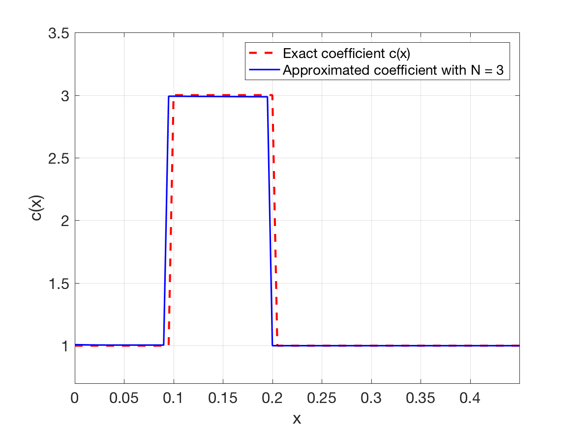
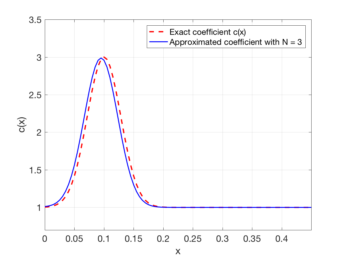
a) $c(x)=1+3\chi[0.1,0.2],$	b) $c(x)=1+2e^{-(x-0.1)^{2}/\left(0.04\right)^{2}}$

Figure 1: Comparison between the exact coefficient $c(x)$ and the approximate coefficient computed by (3.14) with 3 basis functions and exact functions $v_{n}$. The derivative $v^{\prime}_{n}(x)$ is approximated by a finite difference quotient.

In the following examples, to obtain the simulated data we solved the forward problem for $x\in[0,0.5]$ and added a $5\%$ of additive noise to the solution of the forward problem. That means, the noisy data $g_{noisy}(k)$ is calculated as

$$g_{noise}(k)=g_{exact}(k)+0.05|g_{exact}(k)|\cdot\texttt{rand},$$

where $\texttt{rand}\in\left(-1,1\right)$ is a random variable.

In solving the inverse problem, we chose the parameters as follows. Assume that $c(x)$ was unknown on $\left[0,b\right]=[0,0.3]$ only and $c(x)=1$ for $x\notin[0,0.3]$, see (2.3). The interval $[0,0.3]$ was divided into 31 subintervals of equal width $h=0.01$. We chose $11$ wavenumbers uniformly distributed between $\underline{k}=1$ and $\bar{k}=3$. Using numerical tests, we have observed that the coefficient $c(x)$ could be approximated quite accurately using only three terms in the truncated Fourier series (3.9) (see Figure 1). Therefore, the number of basis functions was chosen as $N=3$. The Carleman weight coefficient was chosen as $\lambda=1$ and the regularization parameter was chosen to be $\alpha=10^{-4}$. These parameters were chosen by trial-and-error for a simulated data set. To analyze the reliability of the algorithm, the same parameters were used for all other tests. Finally, the algorithm was started from the initial guess $Q^{(0)}_{h}\equiv 0$ in all of the following examples, except in Figure 4 in which we show the effect of the truncation (3.9) on the reconstruction accuracy of $c(x)$.

Since we assume that $c(x)\geq 1$ for all $x$, we also replaced values of $c(x)$ which are less than 1 by 1. Note that this truncation was done as a post-processing step after the objective functional $J_{h,\lambda,\alpha}$ was minimized. Therefore, it does not affect the inverse algorithm.

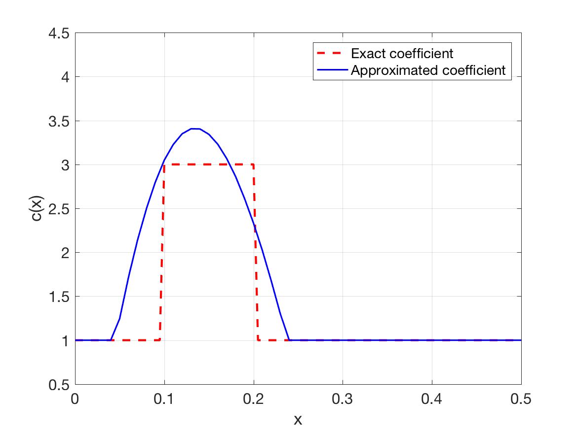
Figure 2: Comparison of the exact and reconstructed coefficient $c(x)$ for Example 1 for $5\%$ noisy data and the initial guess $Q_{h}^{(0)}\equiv 0$.

Example 1. In the first example, we reconstruct a piecewise constant coefficient given by $c(x)=1+3\chi[0.1,0.2],$ where $\chi$ is the characteristic function. The reconstructed coefficient is shown in Figure 2 together with the exact coefficient. In Figure 3, we show the reconstructed functions $V_{n}$, $n=1,2,3$, together with the “exact” ones. The exact functions $V_{n}$ are calculated from the solution of the forward problem with the exact coefficient using (3.1).

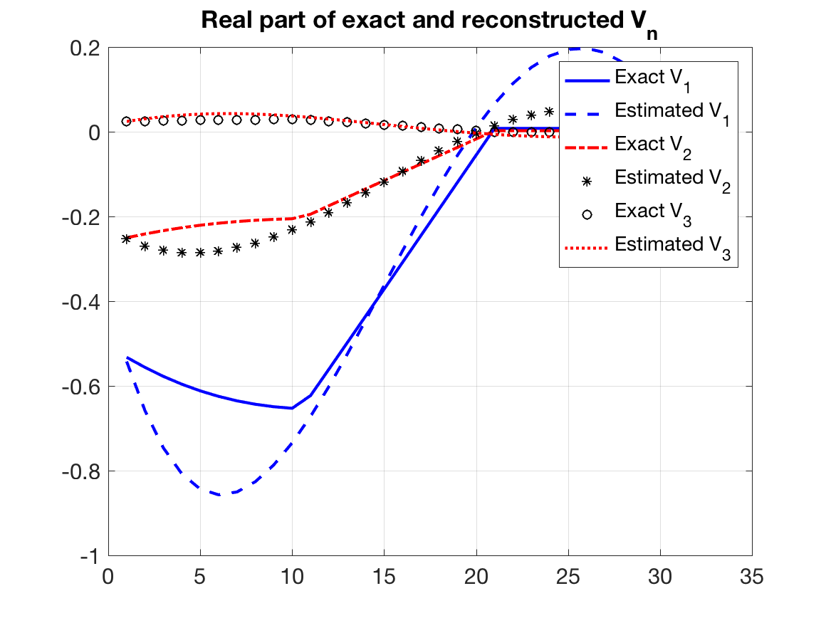
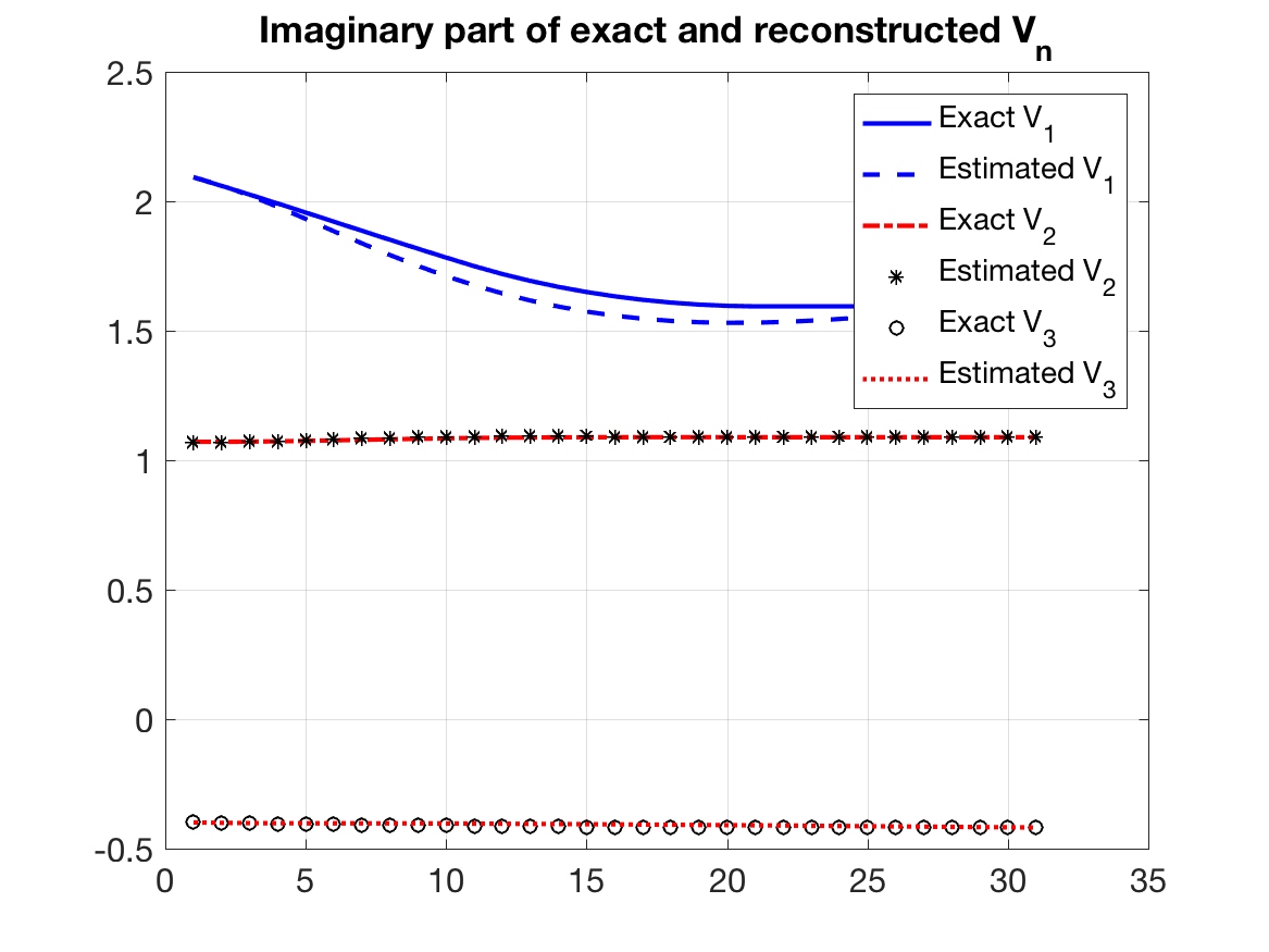
a) Real part	b) Imaginary part

Figure 3: Comparison of the exact and reconstructed functions $V_{n}$ for Example 1 for $5\%$ noisy data and the initial guess $Q_{h}^{(0)}\equiv 0$.

As can be seen from Figure 2, the reconstructed coefficient is a reasonable approximation of the true coefficient. One reason of the difference between the exact and reconstructed coefficients that we have observed through numerical analysis is due to the fact that (3.11) is only an approximation. As a result, the “exact” functions $V_{n}$ are generally not the global minimizer of $J_{h,\lambda,\alpha}$. Therefore, when we minimize $J_{h,\lambda,\alpha}$, we only obtain an approximation of these functions. To confirm this analysis, we show in Figures 4 and 5 the reconstructed coefficient $c(x)$ and the functions $V_{n}$ for noiseless data and with the initial guess $Q^{(0)}_{h}$ calculated from the exact function $V^{*}$. That means, $Q^{(0)}_{h}=V^{*}-\hat{V}^{*}$. Figure 5 indicates that the exact $V_{n}$ are not the globally minimizer of $J_{h,\lambda,\alpha}$ even with noiseless data. Comparison of Figures 2, 3 with Figures 4, 5 also reveals another interesting observation that solutions resulted from the two initial guesses practically coincide. This is exactly the thing which follows from our above theory.

Figure 4: Comparison of the exact and reconstructed coefficient $c(x)$ for Example 1 for noiseless data and with the initial guess $Q_{h}^{(0)}=Q^{*}$.

a) Real part	b) Imaginary part

Figure 5: Comparison of the exact and reconstructed functions $V_{n}$ for Example 1 for noiseless data and with the initial guess $Q_{h}^{(0)}=Q^{*}$.

One simple way to improve the accuracy is to combine this globally convergent algorithm with a locally convergent algorithm, such as the least-squares method. More precisely, we can use the result of this algorithm as an initial guess for the least-squares method. Since we want to focus on the performance of the globally convergent algorithm, we do not discuss the least-squares method here. We refer the reader to [27] for this topic for a similar problem in time domain.

Example 2. In this example, we consider another piecewise constant coefficient with a larger inclusion/background contrast, $c(x)=1+6\chi[0.15,0.25].$ The result is shown in Figures 6 and 7. Even though the jump of the coefficient is high in this case, we still can obtain the contrast quite well.

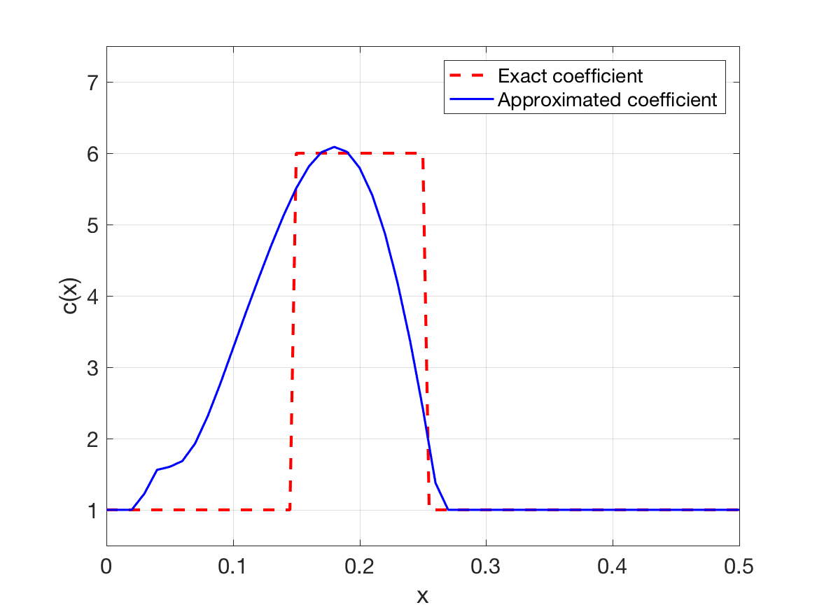
Figure 6: Comparison of the exact and reconstructed coefficient $c(x)$ for Example 2.

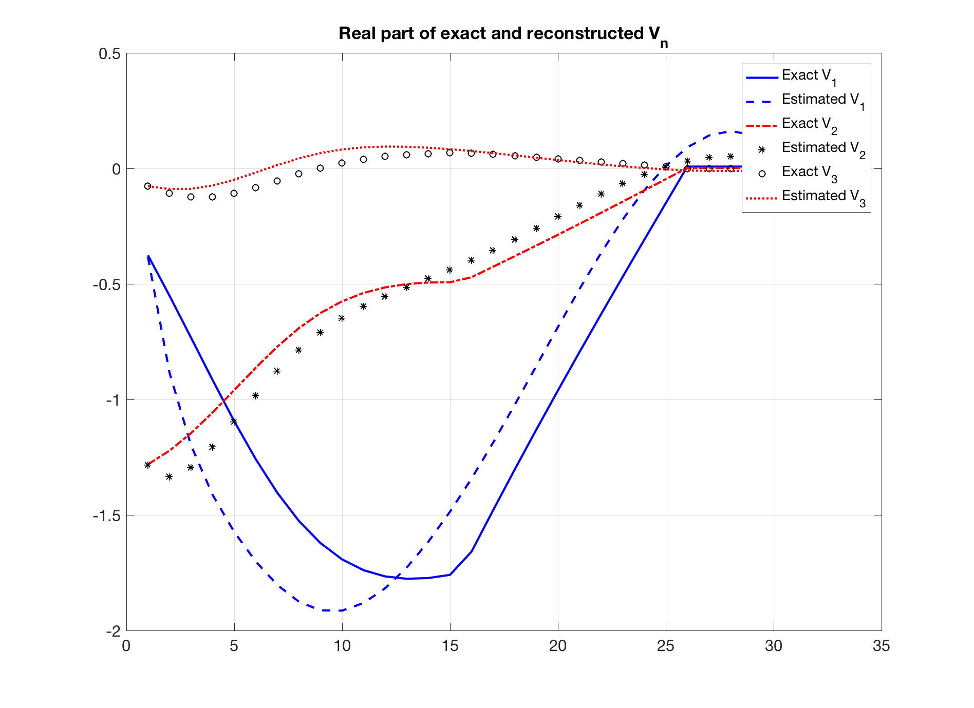
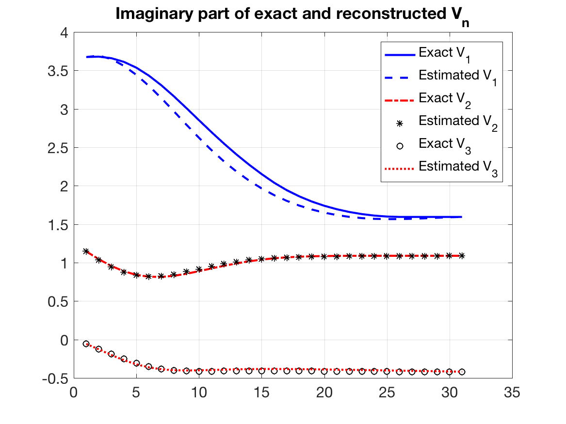
a) Real part	b) Imaginary part

Figure 7: Comparison of the exact and reconstructed functions $V_{n}$ for Example 2.

Example 3. Finally, we consider a continuous coefficient given by $c(x)=1+3e^{-(x-0.1)^{2}/\left(0.04\right)^{2}}.$ Figures 8 and 9 also show a reasonable reconstruction result for both the coefficient $c(x)$ and the functions $V_{n}$.

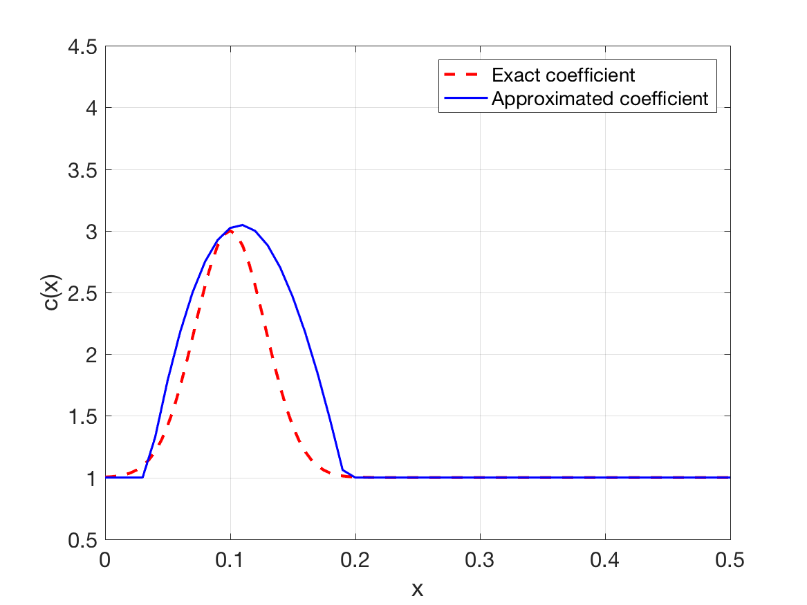
Figure 8: Comparison of the exact and reconstructed coefficient $c(x)$ for Example 3.

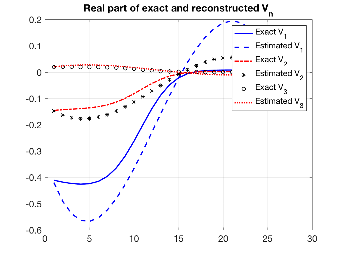
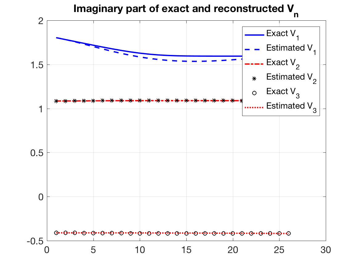
a) Real part	b) Imaginary part

Figure 9: Comparison of the exact and reconstructed functions $V_{n}$ for Example 3.

7 Concluding Remarks

We have proposed a new globally convergent algorithm for the multi-frequency inverse medium scattering problem. The main advantage of this method is that we do not need a good first guess. The numerical examples confirmed that the proposed method provides reasonable reconstruction results. They also confirmed the global convergence of the proposed algorithm because the solutions from different initial guesses are practically the same. As a direct extension of this work, we are considering the 2-d and 3-d problems and will report these cases in our future work.

References

- [1] A. Bakushinskii, M. Klibanov, and N. Koshev. Carleman weight functions for a globally convergent numerical method for ill-posed cauchy problems for some quasilinear PDEs. Nonlinear Analysis: Real World Applications, 34:201–224, 2017.
- [2] G. Bao, P. Li, J. Lin, and F. Triki. Inverse scattering problems with multi-frequencies. Inverse Problems, 31(9):093001, 21, 2015.
- [3] L. Baudouin, M. De Buhan, and S. Ervedoza. Global Carleman estimates for waves and applications. Comm. Partial Differential Equations, 38(5):823–859, 2013.
- [4] L. Beilina and M. V. Klibanov. Globally strongly convex cost functional for a coefficient inverse problem. Nonlinear Analysis: Real World Applications, 22(272–288), 2015.
- [5] K. Belkebir, S. Bonnard, F. P. an P. Sabouroux, and M. Saillard. Validation of 2D inverse scattering algorithms from multi-frequency experimental data. Journal of Electromagnetic Waves and Applications, 14:1637–1667, 2000.
- [6] N. Bleistein. Mathematical methods for wave phenomena. Computer Science and Applied Mathematics. Academic Press, Inc., Orlando, FL, 1984.
- [7] F. Cakoni and D. Colton. Qualitative Methods in Inverse Scattering Theory. Springer, 2006.
- [8] G. Chavent. Nonlinear Least Squares for Inverse Problems. Theoretical Foundations and Step-by-step Guide for Applications. Springer, New York, 2009.
- [9] Y. Chen. Inverse scattering via Heisenberg’s uncertainty principle. Inverse Problems, 13(2):253–282, 1997.
- [10] W. Chew and J. Lin. A frequency-hopping approach for microwave imaging of large inhomogeneous bodies. IEEE Microwave and Guided Wave Letters, 5:439–441, 1995.
- [11] D. Colton and R. Kress. Inverse acoustic and electromagnetic scattering theory. Springer, New York, third edition, 2013.
- [12] D. Colton and P. Monk. The inverse scattering problem for time-harmonic acoustic waves in an inhomogeneous medium. Quart. J. Mech. Appl. Math., 41(1):97–125, 1988.
- [13] D. J. Daniels, editor. Ground Penetrating Radar. The Institute of Electrical Engineers, London, 2004.
- [14] A. V. Goncharsky and S. Y. Romanov. Iterative methods for solving coefficient inverse problems of wave tomography in models with attenuation. Inverse Problems, 33(2):025003, 24, 2017.
- [15] R. Griesmaier. Multi-frequency orthogonality sampling for inverse obstacle scattering problems. Inverse Problems, 27(8):085005, 23, 2011.
- [16] R. Griesmaier and C. Schmiedecke. A factorization method for multifrequency inverse source problems with sparse far field measurements. SIAM J. Imaging Sci., 10(4):2119–2139, 2017.
- [17] B. B. Guzina, F. Cakoni, and C. Bellis. On the multi-frequency obstacle reconstruction via the linear sampling method. Inverse Problems, 26(12):125005, 29, 2010.
- [18] T. Hohage. On the numerical solution of a three-dimensional inverse medium scattering problem. Inverse Problems, 17(6):1743–1763, 2001.
- [19] K. Ito, B. Jin, and J. Zou. A direct sampling method to an inverse medium scattering problem. Inverse Problems, 28(2):025003, 11, 2012.
- [20] K. Ito, B. Jin, and J. Zou. A direct sampling method for inverse electromagnetic medium scattering. Inverse Problems, 29(9):095018, 19, 2013.
- [21] M. V. Klibanov. Convexification of restricted dirichlet-to-neumann map. J. Inverse Ill-posed Problems, 25:669–685, 2017.
- [22] M. V. Klibanov and A. E. Kolesov. Convexification of a 3-d coefficient inverse scattering problem. Computers & Mathematics with Applications, 2018. Published online, https://doi.org/10.1016/j.camwa.2018.03.016.
- [23] M. V. Klibanov, A. E. Kolesov, L. Nguyen, and A. Sullivan. Globally strictly convex cost functional for a 1-D inverse medium scattering problem with experimental data. SIAM J. Appl. Math., 77(5):1733–1755, 2017.
- [24] M. V. Klibanov, A. E. Kolesov, L. Nguyen, and A. Sullivan. A new version of the convexification method for a 1-D coefficeint inverse problem with experimental data. Inverse Problems, 34:115014 (29p), 2018.
- [25] M. V. Klibanov, D.-L. Nguyen, L. H. Nguyen, and H. Liu. A globally convergent numerical method for a 3D coefficient inverse problem with a single measurement of multi-frequency data. Inverse Probl. Imaging, 12(2):493–523, 2018.
- [26] M. V. Klibanov, L. H. Nguyen, A. Sullivan, and L. Nguyen. A globally convergent numerical method for a 1-D inverse medium problem with experimental data. Inverse Probl. Imaging, 10(4):1057–1085, 2016.
- [27] M. V. Klibanov and N. T. Thành. Recovering dielectric constants of explosives via a globally strictly convex cost functional. SIAM J. Appl. Math., 75(2):518–537, 2015.
- [28] A. E. Kolesov, M. V. Klibanov, L. H. Nguyen, D.-L. Nguyen, and N. T. Thành. Single measurement experimental data for an inverse medium problem inverted by a multi-frequency globally convergent numerical method. Appl. Numer. Math., 120:176–196, 2017.
- [29] A. Lakhal. A decoupling-based imaging method for inverse medium scattering for Maxwell’s equations. Inverse Problems, 26(1):015007, 17, 2010.
- [30] J. Li, P. Li, H. Liu, and X. Liu. Recovering multiscale buried anomalies in a two-layered medium. Inverse Problems, 31(10):105006, 28, 2015.
- [31] J. Li, H. Liu, and Q. Wang. Enhanced multilevel linear sampling methods for inverse scattering problems. J. Comput. Phys., 257(part A):554–571, 2014.
- [32] J. Li and J. Zou. A multilevel model correction method for parameter identification. Inverse Problems, 23(5):1759–1786, 2007.
- [33] F. Natterer and F. Wübbeling. A propagation-backpropagation method for ultrasound tomography. Inverse Problems, 11(6):1225–1232, 1995.
- [34] D.-L. Nguyen, M. V. Klibanov, L. H. Nguyen, and M. A. Fiddy. Imaging of buried objects from multi-frequency experimental data using a globally convergent inversion method. J. Inverse Ill-Posed Probl., 26(4):501–522, 2018.
- [35] R. Potthast. A study on orthogonality sampling. Inverse Problems, 26:074015(17pp), 2010.
- [36] G. Rizzuti and A. Gisolf. An iterative method for 2D inverse scattering problems by alternating reconstruction of medium properties and wavefields: theory and application to the inversion of elastic waveforms. Inverse Problems, 33(3):035003, 29, 2017.
- [37] M. Sini and N. T. Thành. Inverse acoustic obstacle scattering problems using multifrequency measurements. Inverse Problems and Imaging, 6(4):749–773, 2012.
- [38] M. Sini and N. T. Thành. Regularized recursive newton-type methods for inverse scattering problems using multifrequency measurements. ESAIM Math. Model. Numer. Anal., 49:459–480, 2015.
- [39] M. Soumekh. Synthetic Aperture Radar Signal Processing. John Wiley & Son, New York, 1999.
- [40] A. Tijhuis, K. Belkebir, A. Litman, and B. de Hon. Multi-frequency distorted-wave Born approach to 2D inverse profiling. Inverse Problems, 17:1635–1644, 2001.
- [41] A. Tijhuis, K. Belkebir, A. Litman, and B. de Hon. Theoretical and computational aspects of 2-D inverse profiling. IEEE Transactions on Geoscience and Remote Sensing, 39(6):1316–1330, 2001.
- [42] F. Vasiliev. Numerical Methods of Solutions of Extremal Problems. Nauka, Moscow, 1989.
- [43] O. Yilmaz. Seismic Data Imaging. Society of Exploration Geophysicists, Tulsa Oklahoma, 1987.