Bose polaron in spherically symmetric trap potentials:
Ground states with zero and lower angular momenta

Abstract

Single-atomic impurities immersed in a dilute Bose gas in the spherically symmetric harmonic trap potentials are studied at zero temperature. In order to find the ground state of the polarons, we present a conditional variational method with fixed expectation values of the total angular momentum operators, $\hat{J}^{2}$ and $\hat{J}_{z}$, of the system, using a cranking gauge-transformation for bosons to move them in the frame co-rotating with the impurity. In the formulation, the expectation value $\langle\hat{J^{2}}\rangle$ is shown to be shared in impurity and bosons, but the value $\langle\hat{J}_{z}\rangle$ is carried by the impurity due to the rotational symmetry. We also analyze the ground-state properties numerically obtained in this variational method for the system of the attractive impurity-boson interaction, and find that excited boson distributions around the impurity overlap largely with impurity’s wave function in their quantum-number spaces and also in the real space because of the attractive interaction employed.

I Introduction

Recently much attention has been devoted to atomic impurities embedded in ultra-cold atomic media because of experimental accessibility of such systems in controlled ways and of observations of various kinds of quasi-particle properties of the impurities : bosonic Catani1 ; Scelle1 ; Hohmann1 ; Compagno1 ; Jrgensen1 ; Hu1 ; Rentrop1 and fermionic Froehlich1 ; Scazza1 ; Cetina1 ones. For instance, the coupling between impurities and medium can be tuned using the Fano-Feshbach resonances between atomic hyperfine states, and the spatial dimensionality or periodicity of the system can also be designed using the effects of external electromagnetic fields PethickSmith1 ; Pitaevskii1 . The quasi-particle energy, width and spectral weight of the impurity can be measured in radiofrequency spectroscopy Jrgensen1 ; Hu1 ; Froehlich1 , and the fine energy splitting of a trapped impurity be measured in the Ramsey spectroscopy with oscillating fields Rentrop1 . Also, the dynamical aspects of the polaron formation can be observed experimentally Cetina1 .

Theoretical studies of such systems have been actively performed prior to the experiments and revealed that properties of impurity are diverse depending on the impurity-medium interaction and medium properties: When the medium is a Bose-Einstein condensate (BEC), the impurity interacting through the Bogoliubov phonon of the medium is called a Bose polaron Cucchietti1 ; Sacha1 ; Tempere1 ; Casteels1 ; Rath1 ; Shashi1 ; Li1 ; Levinsen2 ; Dehkharghani5 ; Ardila2 ; Christensen1 ; Vlietinck1 ; Grusdt1 ; Grusdt3 ; Shchadilova1 ; Shchadilova2 ; Grusdt6 ; Ashida1 ; Ardila6 ; Nielsen3 ; Mistakidis8 ; Mistakidis9 in analogy with that in electron-phonon systems polaronreview1 ; Landau1 ; FPZ1 , where the atomic impurity is a quasiparticle dressed with a virtual cloud of excited phonons. In the case of a degenerate Fermi-gas medium, the impurity is called Fermi polaron Chevy1 ; Massignan1 ; Schirotzek1 ; Ku1 ; Schmidt1 ; Kohstall1 ; Koschorreck1 ; Schmidt6 ; Vlietinck2 ; Trefzger1 ; Trefzger2 ; Massignan5 ; Lan1 ; Lan2 ; Nur1 ; Yi1 ; Parish5 ; Levinsen4 ; Kamikado1 ; Kain1 ; Schmidt5 ; Mistakidis10 , which is dressed with particle-hole excitations around the Fermi surface. In these studies the low energy $s$-wave contact interaction has been frequently used for the impurity-medium interaction. Other kinds of atomic polarons are also studied with unconventional impurity-medium interactions, e.g., $p$-wave interactions Levinsen5 ; Deng1 , dipolar-dipolar interactions Kain3 ; Ardila4 . In the case of the impurity-medium coupling tuned around the unitarity limit, the impurity and medium atoms can form few-body bound states in the medium Levinsen2 ; Shchadilova2 ; Levinsen4 , and consequently the quasi-particle residue almost vanishes. The above mentioned studies entirely assume zero temperature, but recently thermal evolutions of polarons have been investigated, where the medium temperature varies from cold degenerate to hot Boltzmann regimes for Fermi polarons Tajima1 ; Yan8 ; Tajima2 , and, for Bose polarons, the temperature varies over the BEC critical temperature Levinsen8 ; Guenther8 .

In many studies of the polaron that have been done so far, the system is assumed to be spatially uniform, while the real experiments of the ultra-cold gas are usually done on the systems trapped in the harmonic potentials. In the present study, we consider a Bose polaron in spherically symmetric trap in three dimensions, where the angular momentum of the polaron gives the conserved quantum numbers instead of spacial momenta in the uniform system. In particular, we calculate the ground-state energy of a trapped Bose polaron of fixed total angular momentum, and make clear the distributions of the angular-momentum and other quantum numbers of the polaron between the impurity and excited bosons in medium. For this purpose, we develop a variational method with the fixed expectation value of the angular momentum operators.

In Sec. II, we set up our system, and derive a Fröhlich type effective Hamiltonian. In Sec. III, we introduce a cranking gauge transformation, by which all bosons in medium are cranked to move in the co-rotating frame of impurity. In Sec. IV, we develop a variational method to obtain the energy functional for the cranked Hamiltonian, and present variational solutions and distribution functions of the excited bosons. In Sec. V, numerical results and discussion for them are shown. Sec. VI is for the summary and outlook.

II Fröhlich type effective Hamiltonian

We consider the system of a single atomic impurity interacting with a dilute Bose gas, where the impurity and the gas are trapped in the spherically-symmetric harmonic potentials with the same centers. The impurity and bosons are all spinless, so that the total orbital angular momentum of the system is conserved. We also suppose that bosons are non-interacting, while the impurity-boson interaction is tuned finite by the Feshbach resonance method. Thus, when the interaction is turned off, all medium bosons occupy the lowest energy state of the trap potential to form a $T=0$ BEC. This system is described by the following effective Hamiltonian:

$$\mathcal{H}({\bf r}) = H_{ho}({\bf r})+\int_{{\bf r}^{\prime}}\,\phi^{\dagger}({\bf r}^{\prime})\left[-\frac{\hbar^{2}{\nabla^{\prime}}^{2}}{2m_{b}}+\frac{m_{b}\omega_{b}^{2}}{2}{r^{\prime}}^{2}\right]\phi({\bf r}^{\prime})$$ (1)

$$+g\int_{{\bf r}^{\prime}}\,\phi^{\dagger}({\bf r}^{\prime})\delta^{(3)}({\bf r}-{\bf r}^{\prime})\phi({\bf r}^{\prime})$$

$$= H_{ho}({\bf r})+\sum_{s}E_{s}^{b}b_{s}^{\dagger}b_{s}+g\sum_{s,s^{\prime}}\phi_{s}^{b*}({\bf r})\phi_{s^{\prime}}^{b}({\bf r})b_{s}^{\dagger}b_{s^{\prime}}$$

where the freedoms of the impurity and medium boson are represented in the first and the second quantized form. We have used the abbreviated notation for the spacial integral: $\int_{{\bf r}}\equiv\int{\rm d}{\bf r}^{3}$. The first term $H_{ho}({\bf r})$ is the Hamiltonian of the impurity trapped in the harmonic-oscillator potential:

$$H_{ho}({\bf r}) = -\frac{\hbar^{2}}{2m_{I}}\frac{1}{r^{2}}\partial_{r}\left(r^{2}\partial_{r}\right)+\frac{\hbar^{2}{\hat{L}}^{2}}{2m_{I}\,r^{2}}+\frac{m_{I}\omega_{I}^{2}}{2}r^{2}$$ (2)

where $(r,\theta,\varphi)$ is the spherical coordinate of the impurity, and $m_{I}$ and $\omega_{I}$ is the impurity mass and the angular frequency of the trap. The squared orbital angular-momentum operator ${L}^{2}$ is represented by,

$${\hat{L}}^{2}=-\left[\frac{1}{\sin\theta}\partial_{\theta}\left(\sin\theta\partial_{\theta}\right)+\frac{1}{\sin^{2}\theta}\partial_{\varphi}^{2}\right],$$

The second term in (1) represents the Hamiltonian of the medium boson; the $m_{b}$ and $\omega_{b}$ are the mass and the trap angular frequency of the medium boson, and the coupling constant $g$ of the impurity-medium contact interaction is given by the s-wave scattering length $a$ as $g=2\pi a/m_{r}$ in low-temperature approximation. The second line of (1) is obtained with the substitution of the field operator expansion: $\phi({\bf r}^{\prime})=\sum_{s}\phi_{s}^{b}({\bf r}^{\prime})b_{s}$ where the $\phi_{s}^{b}({\bf r})$ are the eigenfunctions of the harmonic oscillator potential for the eigenvalues $E^{b}_{s}$, and the $b_{s}$ and $b_{s}^{\dagger}$ are the corresponding bosonic annihilation and creation operators. The label $s$ representing the medium-boson states is the abbreviated notation for $s=(n,l,m)$: the principal, the azimuthal, and the magnetic quantum numbers, respectively.

The explicit form of the Harmonic-oscillator eigenfunctions $\phi^{\alpha}_{s}({\bf r})$ for the medium boson ($\alpha=b$) and the impurity ($\alpha=I$) are denoted as,

$$\phi_{s}^{\alpha}({\bf r})=R^{\alpha}_{nl}(r)Y_{lm}(\theta,\varphi),$$ (3)

where the angular part $Y_{lm}$ is the spherical harmonic $Y$-function, and the radial part $R^{\alpha}_{nl}(r)$ are,

$$R^{\alpha}_{nl}(r) ={\mathcal{N}}_{n,l}\left(m_{\alpha}\omega_{\alpha}\right)^{\frac{3}{4}}\,\left(\sqrt{m_{\alpha}\omega_{\alpha}}r\right)^{l}\,e^{-\frac{m_{\alpha}\omega_{\alpha}}{2}r^{2}}L^{\left(\frac{1+2l}{2}\right)}_{n}\left(m_{\alpha}\omega_{\alpha}r^{2}\right),$$ (4)

$${\mathcal{N}}_{nl} =\sqrt{\frac{2^{n+l+2}n!}{\sqrt{\pi}\left(2n+2l+1\right)!!}}.$$ (5)

The Laguerre function $L_{n}^{(k)}(x)$ that we use in this paper is defined by

$$L_{n}^{(k)}(x)=\frac{e^{x}x^{-k}}{n!}\frac{{\rm d}^{n}}{{\rm d}x^{n}}\left(e^{-x}x^{n+k}\right).$$

The energy-eigenvalue corresponding to the state (3) is

$$E_{nl}^{\alpha}=\frac{\omega_{\alpha}\hbar}{2}(3+2l+4n).$$ (6)

It should be noticed that we use the unit system of $\hbar=1$ throughout this paper.

II.1 Bogoliubov approximation and Fröhlich type Hamiltonian

In the case of the small number excitation of medium bosons around the impurity in comparison with the total condensed boson number $N_{0}$ Bruderer1 ; Nakano2 , we can use the Bogoliubov approximation $b_{0}\simeq\sqrt{N_{0}}$, where $s=0$ corresponds to the lowest energy level ($n=l=0$). With keeping terms in the interaction part up to the linear order of the excited boson, we obtain

$$\mathcal{H}({\bf r}) \simeq H_{ho}({\bf r})+E^{b}_{0}N_{0}+\sum_{s\neq 0}E_{s}^{b}b_{s}^{\dagger}b_{s}+gN_{0}|\phi_{0}^{b}({\bf r})|^{2}$$ (7)

$$\ +g\sqrt{N_{0}}\sum_{s\neq 0}\left[\Phi_{s}({\bf r})b_{s}+\Phi_{s}^{*}({\bf r})b_{s}^{\dagger}\right],$$

where

$$\Phi_{s=\left\{n,l,m\right\}}({\bf r})\equiv\sqrt{\frac{1}{4\pi}}R_{00}^{b}(r)R_{nl}^{b}(r)Y_{lm}(\theta,\varphi).$$

The Hamiltonian (7) can be transformed into the same form of the Fröhlich Hamiltonian of the electron-phonon system, and the electron polaron was originally studied in FPZ1 for the polar crystals. We will use the Hamiltonian (7) in the present paper.

III Cranking of boson states

In the present study we aim to find the lowest energy state of the Hamiltonian (7) for given expectation values of the total angular momentum operators. These states correspond to the yrast states appeared in the description of rotational collective excitations of an axially deformed nucleus in nuclear physics, where the rotation axis is not parallel to that of the axially symmetry, and the gauge transformation (cranking) $e^{i\omega_{k}t\hat{J}_{k}}$ is introduced conveniently to shift the state from the normal space-fixed frame to the co-rotating frame with the nucleons in which the nucleus wave function is stationary Rowe1 ; Inglis1 ; Thouless1 . The same method can also be utilized in the present case to describe the excitations of bosons around the impurity; we rotate the boson cloud around the impurity collectively by the gauge transformation ($S$ transformation) with the solid angle variables $(\theta,\varphi)$ of the impurity:

$$S(\varphi,\theta) = e^{-i\varphi\hat{M}_{z}}e^{-i\theta\hat{M}_{y}}$$ (8)

where the boson angular-momentum operator is defined by

$$\hat{M}_{i}=\sum_{n,l,m,m^{\prime}}b_{nlm}^{\dagger}\left(\hat{\mathcal{L}}_{i}\right)_{m,m^{\prime}}^{(l)}b_{nlm^{\prime}}$$ (9)

where $\left(\hat{\mathcal{L}}_{i}\right)_{m,m^{\prime}}^{(l)}$ is the matrix element of a general orbital angular momentum operator $\hat{\mathcal{L}}_{i}$ by the eigen-states of rank $l$ :

$$\left(\hat{\mathcal{L}}_{i}\right)_{m,m^{\prime}}^{(l)}\equiv\langle l,m|\hat{\mathcal{L}}_{i}|l,m^{\prime}\rangle,$$

$$\quad l=0,1,2,\cdots,\quad m,m^{\prime}=-l,-1+1,\cdots,l-1,l.$$

The general form of this transformation has been successfully introduced by Schmidt and Lemeshko to investigate the angular momentum distribution in the system of a linear rotor impurity embedded in bosonic environment in free space Lemeshko3 ; Lemeshko4 ; Lemeshko7 , and the simpler version, $S(\varphi,0)$, has been utilized in the system of Bose polaron in axially symmetric trap potentials for the study of the angular-momentum drag effect NYI1 .

III.1 Cranked angular momentum operators

The $S$-transformation practically serves as linear transformations for the boson annihilation operators and the boson angular-momentum operators:

$$S^{-1}b_{nlm}S = \sum_{m^{\prime}=-l,\cdots,l}D^{l}_{m,m^{\prime}}\left(\varphi,\theta,0\right)b_{nlm^{\prime}},$$ (10)

$$S^{-1}\hat{M}_{i}S = \sum_{j=0,\pm 1}{D^{1}_{i,j}}^{*}\left(\varphi,\theta,0\right)\hat{M}_{j},$$ (11)

where we have used the spherical basis: $\hat{M}_{0}=\hat{M}_{z}$ and $\hat{M}_{\pm 1}=\mp\frac{1}{\sqrt{2}}\left(\hat{M}_{x}\pm i\hat{M}_{y}\right)$, for vector indices, and Wigner’s $D$ function with Euler angles $(\alpha,\beta,\gamma)$ for the spacial rotation Rose1 :

$$D^{l}_{m,m^{\prime}}\left(\alpha,\beta,\gamma\right)=\langle l,m|e^{-i\alpha\hat{\mathcal{L}}_{z}}e^{-i\beta\hat{\mathcal{L}}_{y}}e^{-i\gamma\hat{\mathcal{L}}_{z}}|l,m^{\prime}\rangle.$$ (12)

The $S$ transformation acts as a shift operator for the impurity angular-momentum operators:

$$S^{-1}\hat{L}_{0}S = \hat{L}_{0}+S^{-1}\left(\hat{L}_{0}S\right)=\hat{L}_{0}-S^{-1}\hat{M}_{z}S,$$ (13)

$$S^{-1}\hat{L}_{\pm 1}S = \hat{L}_{\pm 1}+S^{-1}\left(\hat{L}_{\pm 1}S\right)$$ (14)

$$= \hat{L}_{\pm 1}+\frac{1}{\sqrt{2}}e^{\pm i\varphi}S^{-1}\left[i\,e^{-i\varphi\hat{M}_{z}}\hat{M}_{y}e^{i\varphi\hat{M}_{z}}\mp\cot\theta\hat{M}_{z}\right]S,$$

where we have used the spherical-basis representation:

$$\hat{L}_{0} = \hat{L}_{z}=-i\partial_{\varphi},$$ (15)

$$\hat{L}_{\pm 1} = \mp\frac{1}{\sqrt{2}}\left(\hat{L}_{x}\pm i\hat{L}_{y}\right)=\frac{1}{\sqrt{2}}e^{\pm i\varphi}\left(-\partial_{\theta}\mp i\,\cot{\theta}\partial_{\varphi}\right).$$ (16)

In the present system, the total angular momentum operator of the system is given by

$$\hat{J}_{i}=\hat{L}_{i}+\hat{M}_{i},$$ (17)

and the $z$-th component $\hat{J}_{z}$ and the squared amplitude $\hat{J}^{2}$ are conserved: $\left[\hat{J}_{z},{\mathcal{H}}({\bf r})\right]=\left[\hat{J}^{2},{\mathcal{H}}({\bf r})\right]=\left[\hat{J}_{z},\hat{J}^{2}\right]=0$. Using the transformation formulas of the angular momentum operators $\hat{M}_{i}$ and $\hat{L}_{i}$, the $S$-transformed operators of $\hat{J}_{z}$ and $\hat{J}^{2}$ becomes,

$$S^{-1}\hat{J}_{z}S = S^{-1}(\hat{L}_{z}+\hat{M}_{z})S=\hat{L}_{z},$$ (18)

$$S^{-1}\hat{J}^{2}S = S^{-1}\left(\hat{L}^{2}+\hat{M}^{2}+2\hat{M}\cdot\hat{L}\right)S$$ (19)

$$= \hat{L}^{2}+\hat{O}_{L}+\hat{M}^{2}$$

$$+2\sum_{i,j=0,\pm 1}\hat{M}_{j}^{\dagger}{D^{1}_{i,j}}(\varphi,\theta,0)\left[S^{-1}(\hat{L}_{i}S)+\hat{L}_{i}\right],$$

where we used the scalar product $\hat{M}\cdot\hat{L}=\sum_{i=0,\pm 1}\hat{M}_{i}^{\dagger}\hat{L}_{i}$ in the spherical basis representation, and the shift operator $\hat{O}_{L}$ of $\hat{L}^{2}$ is defined by

$$\hat{O}_{L}:=S^{-1}\hat{L}^{2}S-\hat{L}^{2}=S^{-1}\left(\hat{L}^{2}S\right)+2S^{-1}(\hat{L}S)\cdot\hat{L}.$$ (20)

We see from the results (18) and (19) that the $z$-component of the total angular momentum is taken over solely by the impurity after the $S$ transformation, while the total angular momentum of the system looks complicated.

III.2 Cranked Hamiltonian

In similar calculation, the $S$-transformation of the Hamiltonian (7) is obtained,

$$S^{-1}{\mathcal{H}}({\bf r})S = H_{ho}({\bf r})+\frac{\hat{O}_{L}}{2m_{I}r^{2}}+\sum^{\prime}_{n,l,m}E_{nl}^{b}b^{\dagger}_{nlm}b_{nlm}$$ (21)

$$+E^{b}_{00}N_{0}+gN_{0}|\phi_{0}^{b}({\bf r})|^{2}$$

$$+g\frac{\sqrt{N_{0}}}{4\pi}R_{00}^{b}(r)\sum^{\prime}_{n,l}\sqrt{2l+1}R_{nl}^{b}(r)\left(b_{nl0}+b^{\dagger}_{nl0}\right),$$

where the symbols $\sum^{\prime}_{n,l,m}$ and $\sum^{\prime}_{n,l}$ represent the summations except $n=l=m=0$ and $n=l=0$ respectively. In the derivation, we have used the formula $Y_{lm}^{*}(\theta,\varphi)=\sqrt{\frac{2l+1}{4\pi}}D_{m,0}^{l}(\varphi,\theta,0)$ and the orthogonality of the $D$ functions Rose1 . The second term including the shift operator $\hat{O}_{L}$ corresponds to the rotation energy of the impurity, which comes from the rotation energy of excited bosons originally before the cranking. The last term is that of the boson-impurity coupling; it should be noticed that it includes the coupling with the excited bosons with $m=0$ in the $S$-transformed HamiltonianLemeshko3 ; Lemeshko4 .

IV Variational method

Let’s develop the variational method to obtain the lowest energy states under the condition that the azimuthal and $z$ (magnetic) components of the total angular momentum are given by the expectation values $(J,J_{z})$. The Hamiltonian (21) shows that the impurity-boson interaction term includes only the excited bosons with $m=0$ after the $S$-transformation, so that, as a variational state of excited bosons around the impurity, we employ the coherent state for the excited bosons with the quantum numbers $s=(n,l,0)$: LLP1 ; Schweber1 ,

$$\left|b\right\rangle = \exp\sum^{\prime}_{n,l}\left(f_{nl}b_{nl0}^{\dagger}-f_{nl}^{*}b_{nl0}\right)\left|0\right\rangle,$$ (22)

where the variational parameters $f_{nl}$ and $f_{nl}^{*}$ are eigenvalues of annihilation and creation operators: $b_{nl0}\left|b\right\rangle=f_{nl}\left|b\right\rangle$, $\left\langle b\right|b_{nl0}^{\dagger}=\left\langle b\right|f_{nl}^{*}$. The state $\left|b\right\rangle$ is a normalized one: $\langle b|b\rangle=1$. It would be a good approximation for the heavy impurity trapped in the deep potential; in the case of heavy mass or high trap-frequency limits of the impurity, the above coherent state becomes the exact solution because the impurity becomes localized at the center of trap.

Now we use the abbreviated notation for the expectation value of operator by the coherent state $\left|b\right\rangle$ as $\langle\cdots\rangle_{b}\equiv\langle b|\cdots|b\rangle$. Then that of the transformed Hamiltonian (21) and the $S$-transformed total angular momentum operators become,

$$\langle S^{-1}{\mathcal{H}}({\bf r})S\rangle_{b} = H_{ho}^{f}({\bf r})+\sum_{n,l}^{\prime}\left[\frac{l(l+1)}{2m_{I}r^{2}}+E_{nl}^{b}\right]|f_{nl}|^{2}$$ (23)

$$+E^{b}_{00}N_{0}+gN_{0}|\phi_{0}^{b}({\bf r})|^{2}$$

$$+g\frac{\sqrt{N_{0}}}{4\pi}R_{00}^{b}(r)\sum_{n,l}^{\prime}\sqrt{2l+1}R_{n,l}^{b}(r)\left(f_{nl}+f^{*}_{nl}\right),$$

$$\langle S^{-1}\hat{J}^{2}S\rangle_{b} = \hat{L}^{2},$$ (24)

$$\langle S^{-1}\hat{J}_{z}S\rangle_{b} = \hat{L}_{z},$$ (25)

where we have used the expectation value $\langle\hat{O}_{L}\rangle_{b}=\sum_{n,l}^{\prime}l(l+1)|f_{nl}|^{2}$.

The expectation value (23), where the bosonic degrees of freedom have been eliminated, provide the effective Hamiltonian of the impurity, and eqs. (24) and (25) are the corresponding effective total angular-momentum operators represented with the impurity coordinate. It is very interesting that the latter are the same with the impurity angular momentum; it gives an essential advantage in the present variational method with the condition of the fixed total angular momentum.

IV.1 Variational states of impurity

Since the total angular momentum operators (24) and (25) are given by those of the impurity, the variational state of the impurity can be assumed as the eigenfunctions (3) of the impurity with fixed azimuthal and magnetic quantum numbers $(J,J_{z})$:

$$\Psi_{JJ_{z}}({\bf r})=\sum_{n}F_{nJJ_{z}}\,\phi^{I}_{nJJ_{z}}({\bf r})$$ (26)

where $J_{z}=-J,-J+1,\cdots,J-1,J$ and the coefficients $F_{nJJ_{z}}$ serve as Ritz-type variational parameters. Note that we do not consider mixing of different angular momenta, because of rotational symmetry. Since the states with large principal quantum numbers less contribute in the ground state in the weak coupling regime, we truncate the variational state up to $n=1$ in the present calculation:

$$\Psi_{JJ_{z}}({\bf r})=\sum_{n=0,1}F_{nJ}\,\phi^{I}_{nJJ_{z}}({\bf r}).$$ (27)

Note that the subscript $J_{z}$ has been omitted in the variational parameters since the rotational symmetry of the system gives the degeneracy for the direction in real space and the variational parameters do not depend on $J_{z}$. In solving the variational equations, we impose the normalization condition for the parameters: $|F_{0J}|^{2}+|F_{1J}|^{2}=1$.

IV.2 Variational energy functional and solutions

Now taking the expectation value of the Hamiltonian (23) with respect to the impurity’s variational state (27), we obtain the variational energy functional for the state with the total angular momentum $(J,J_{z})$:

$$E\left[F_{nJ};f_{nl}\right] = \langle{\mathcal{H}}({\bf r})\rangle_{JJ_{z}}$$ (28)

$$= E^{I}_{0J}|F_{0J}|^{2}+E^{I}_{1J}|F_{1J}|^{2}+E^{b}_{00}N_{0}\left(|F_{0J}|^{2}+|F_{1J}|^{2}\right)$$

$$+\sum_{n,l}^{\prime}\left[E_{nl}^{b}\left(|F_{0J}|^{2}+|F_{1J}|^{2}\right)+\frac{l(l+1)}{2m_{I}}G[F_{0J};F_{1J}]\right]|f_{nl}|^{2}$$

$$+g\frac{N_{0}}{4\pi}H[F_{0J};F_{1J}]_{00}$$

$$+g\frac{\sqrt{N_{0}}}{4\pi}\sum_{n,l}^{\prime}\sqrt{2l+1}\left[H[F_{0J};F_{1J}]_{nl}f_{nl}+H[F_{0J};F_{1J}]_{nl}^{*}f^{*}_{nl}\right],$$

where we have defined the functionals:

$$G[F_{0J};F_{1J}] = \int_{\bf r}\frac{1}{r^{2}}\left|\sum_{n=0,1}F_{nJ}\phi^{I}_{nJJ_{z}}({\bf r})\right|^{2},$$ (29)

$$H[F_{0J};F_{1J}]_{nl} = \int_{\bf r}{R_{00}^{b}(r)}R_{nl}^{b}(r)\left|\sum_{n=0,1}F_{nJ}\phi^{I}_{nJJ_{z}}({\bf r})\right|^{2}.$$ (30)

The variational equation $\delta E/\delta f_{nl}^{*}=0$ gives the formal solution:

$$\bar{f}_{nl}[F_{0J};F_{1J}]=-g\frac{\sqrt{N_{0}}}{4\pi}\frac{\sqrt{2l+1}H[F_{0J};F_{1J}]_{nl}^{*}}{E_{nl}^{b}\left(|F_{0J}|^{2}+|F_{1J}|^{2}\right)+\frac{l(l+1)}{2m_{I}}G[F_{0J};F_{1J}]},$$ (31)

and, plugging it back to the variational energy (28), we obtain

$$E[F_{nJ};\bar{f}_{nl}] =E^{I}_{0J}|F_{0J}|^{2}+E^{I}_{1J}|F_{1J}|^{2}$$

$$+E^{b}_{00}N_{0}\left(|F_{0J}|^{2}+|F_{1J}|^{2}\right)+g\frac{N_{0}}{4\pi}H[F_{0J};F_{1J}]_{00}$$

$$-g^{2}\frac{N_{0}}{(4\pi)^{2}}\sum_{n,l}^{\prime}(2l+1)\frac{|H[F_{0J};F_{1J}]_{nl}|^{2}}{E_{nl}^{b}\left(|F_{0J}|^{2}+|F_{1J}|^{2}\right)+\frac{l(l+1)}{2m_{I}}G[F_{0J};F_{1J}]}.$$

Since the coefficients appearing in the variational energy are all real, the solutions of $F_{0J}$ and $F_{1J}$ are also found to be real. Using the normalization condition $F_{0J}=\sqrt{1-F_{1,J}^{2}}$ and the analytical expression of $G[F_{0J};F_{1J}]$, we finally obtain

$$E[F_{1J}] =E^{I}_{0J}+E^{b}_{00}N_{0}+\left(E^{I}_{1J}-E^{I}_{0J}\right)F_{1J}^{2}+E_{\rm bg}[F_{1J}]+E_{\rm int}[F_{1J}],$$ (32)

where the background interaction energy is,

$$E_{\rm bg}[F_{1J}]\equiv g\frac{N_{0}}{4\pi}\left[H_{00J}^{0}+2F_{1J}\sqrt{1-F_{1J}^{2}}H_{00J}^{c}+F_{1J}^{2}\left(H_{00J}^{1}-H_{00J}^{0}\right)\right],$$ (33)

which comes from the interaction between impurity and background condensed bosons corresponding to the term $gN_{0}|\phi^{b}_{0}({\bf x})|^{2}$ in (23). The interaction energy term $E_{\rm int}[F_{1J}]$ is represented as

$$E_{\rm int}[F_{1J}]\equiv-\frac{g^{2}N_{0}}{(4\pi)^{2}}\sum_{n,l}^{\prime}(2l+1)\frac{\left[H_{nlJ}^{0}+2F_{1J}\sqrt{1-F_{1J}^{2}}H_{nlJ}^{c}+F_{1J}^{2}\left(H_{nlJ}^{1}-H_{nlJ}^{0}\right)\right]^{2}}{E_{nl}^{b}+\frac{l(l+1)}{2J+1}\omega_{I}\left[1+2F_{1J}\sqrt{1-F_{1J}^{2}}/\sqrt{J+\frac{3}{2}}\,\right]},$$ (34)

which is traced back to the parts including $f_{nl}$ in the second and the last terms in (23), and corresponds to the interaction between the impurity and the excited bosons. The explicit forms of the coefficients $H_{nlJ}^{0},H_{nlJ}^{c},H_{nlJ}^{1}$ in $E_{\rm bg}$ and $E_{\rm int}$ are shown also in Appendix B.

In experiments, the energy shift, i.e., the energy with bare impurity and background BEC contributions being subtracted, is measurable using the radio-frequency spectroscopy Jrgensen1 ; Hu1 ; in the present theory, it is given by the formula:

$$\Delta E[F_{1J}]\equiv\left(E^{I}_{1J}-E^{I}_{0J}\right)F_{1J}^{2}+E_{\rm bg}[F_{1J}]+E_{\rm int}[F_{1J}].$$ (35)

IV.3 Comparison with the second order perturbation theory

In general, the solutions of variational method in the present method includes non-perturbative effects, but it is heuristic and interesting to see its perturbative nature before going into numerical results. Expanding the variational solution (32) with the coupling constant $g$, we obtain $F_{1J}=-g\frac{N_{0}}{4\pi}\frac{H_{00J}^{c}}{E^{I}_{1J}-E^{I}_{0J}}$, to the leading order of $g$; then the ground state energy becomes

$$E = E^{I}_{0J}+E^{b}_{00}N_{0}+g\frac{N_{0}}{4\pi}H_{00J}^{0}-g^{2}\frac{N_{0}^{2}}{(4\pi)^{2}}\frac{\left(H_{00J}^{c}\right)^{2}}{E^{I}_{1J}-E^{I}_{0J}}$$ (36)

$$\quad-g^{2}\frac{N_{0}}{(4\pi)^{2}}\sum_{n,l}^{\prime}\frac{(2l+1)\left(H_{nlJ}^{0}\right)^{2}}{E_{nl}^{b}+\frac{l(l+1)}{2J+1}\omega_{I}}.$$

to the order of $g^{2}$. The result should be compared with that of the second-order perturbation theory; for the ground state energy of $J=0$:

$$\langle{\mathcal{H}}\rangle \simeq E_{00}^{I}+E_{00}^{b}N_{0}+g\frac{N_{0}}{4\pi}H_{000}^{0}-g^{2}\frac{N_{0}^{2}}{(4\pi)^{2}}\frac{\left(H_{000}^{c}\right)^{2}}{E_{10}^{I}-E_{00}^{I}}$$ (37)

$$-g^{2}\frac{N_{0}}{\left(4\pi\right)^{2}}\sum_{n\neq 0}\left(\frac{\left(H_{n00}^{c}\right)^{2}}{E_{10}^{I}-E_{00}^{I}+E_{n0}^{b}}+\frac{\left(H_{n00}^{0}\right)^{2}}{E_{n0}^{b}}\right).$$

Comparing (36) with (37), we find that differences appear in the $g^{2}N_{0}$ term, which is attributed to the Fröhlich-type boson-impurity interaction. In the denominator of (36), the energy of impurity’s intermediate states in (37) is replaced by an averaged rotation energy $\frac{l(l+1)}{2J+1}\omega_{I}$. It can be explained from the cranking transformation and the angular momentum conservation: after cranking transformation, all bosons stop to be in rotating states, and the impurity rotates instead in order to satisfy the angular momentum conservation; consequently its effect appears as the rotation energy. In the perturbation theory for the ground state, the impurity and bosons intermediate virtual states are taken in the order from those of low-energy regardless of the angular momentum conservation.

IV.4 Distribution functions of excited bosons and quasiparticle residue

Since the quasi-particle properties of the Bose polaron are characterized by the virtual boson excitations around the impurity, the number of excited bosons around the poralon is an important quantity. The excited-boson number $N_{nlm}^{JJ_{z}}$ of bosons with quantum numbers $(n,l,m)$ for the polaron with the total angular momentum $(J,J_{z})$ is given by

$$N_{nlm}^{JJ_{z}} = \langle b_{nlm}^{\dagger}b_{nlm}\rangle_{JJ_{z}}$$ (38)

$$= \int{\rm d}\theta\sin\theta{\rm d}\varphi\,|Y_{JJ_{z}}\left(\theta,\varphi\right)|^{2}\left|D^{l}_{m,0}\left(\varphi,\theta,0\right)\right|^{2}\langle b|b_{nl0}^{\dagger}b_{nl0}|b\rangle$$

$$= \left|f_{nl}\right|^{2}\sum_{L=|J-l|}^{J+l}\braket{l0;L0}{J0}^{2}\,\braket{JJ_{z};lm}{LJ_{z}+m}^{2}.$$

It should be noted that the dependence on $J_{z}$ and $m$ in $N_{nlm}^{JJ_{z}}$ comes through the Clebsch-Gordan coefficients $\braket{l0;L0}{J0}$ and $\braket{JJ_{z};lm}{LJ_{z}+m}$ which are originated in the averaged overlap of the coupled angular-momentum states from $J$ and $l$. The dependence through the Clebsch-Gordan coefficients is not dynamical but kinematical; it can be understood from independence of the polaron energy-functional on $J_{z}$ or $m$.

From (38), we obtain the total excited-boson number by summing up quantum numbers:

$$N_{b}^{J} = \sum^{\prime}_{n,l}\sum_{m=-l,\cdots,l}N_{nlm}^{JJ_{z}}=\sum^{\prime}_{n,l}\left|f_{nl}\right|^{2}.$$ (39)

It is clear that the total number does not depend on $J_{z}$ but it has the implicit $J$-dependence through the variational parameter $F_{1J}$.

The real-space density distribution of the excited bosons is given by the expectation value:

$$\left\langle\phi^{b\,\dagger}({\bf x})\phi^{b}({\bf x})\right\rangle_{JJ_{z}} = \sum^{\prime}_{n,l}\sum_{m=-l,\cdots,l}N_{nlm}^{JJ_{z}}\,|\phi^{b}_{nlm}({\bf x})|^{2}.$$ (40)

For the angular momentum, the boson contribution is found to vanish,

$$\langle\hat{M}_{i}\rangle_{JJ_{z}}=0,$$ (41)

which implies that the impurity alone bears the contribution for $J_{z}$; it shows that no drag effects exist for the angular momentum unlike the axial symmetric case NYI1 . There are two reasons for this property. First, thanks to the complete rotational symmetry the energy functional becomes spherically symmetric and does not depend on $J_{z}$. Second, no angular-momentum exchange can happen between impurity and bosons through the impurity-boson interaction because a density-density type interaction is employed in this work. In order for $\langle\hat{M}_{i}\rangle$ to be finite, an asymmetry with respect to $m$ is required in the distribution function of excited bosons, but there is no sources of the asymmetry in the present case because of the rotational symmetry. In the case of axial symmetric trap potentials, this specific axis provides an asymmetry for the energy functional and the distribution function NYI1 . We will come back to this point when we present the numerical results in the next section.

The quasi-particle residue is defined as

$$Z_{J} = \left|\int_{\bf r}\phi_{0JJ_{z}}^{I*}({\bf r})\langle 0|S|b\rangle\Psi_{JJ_{z}}({\bf r})\right|^{2}=|F_{0J}|^{2}e^{-\sum_{n,l}^{\prime}|f_{nl}|^{2}}.$$ (42)

It also quantifies the modification of the impurity due to the interaction effects, which is given by the overlap between the bare and interacting impurity states with the angular momentum $(J,J_{z})$. Eq. (42) shows that the residue is factorized into the ground state component of the impurity wave function $|F_{0J}|^{2}$ and a weight factor $e^{-\sum_{n,l}^{\prime}|f_{nl}|^{2}}$ of the excited bosons, while in the spatially uniform case it depends only on the latter.

V Numerical results and discussion

In numerical calculation we take K⁴⁰ as the impurity immersed in medium bosons of Rb⁸⁷; the trap frequencies of the impurity and the medium bosons and the condensed-boson number that we take are

$$\omega_{I}=200\,{\rm Hz},\quad\omega_{b}=100\,{\rm Hz},\quad N_{0}=10^{4},$$ (43)

throughout numerical calculations. We treat the boson-impurity scattering length as a variable parameter, but neglect the boson-boson scattering length in the present calculation. In actual experiments of Bose polarons Jrgensen1 ; Hu1 , the trap potentials for impurity and medium-bosons are both axially symmetric, and the boson-boson scattering length is usually set to be a small positive number to stabilize the boson sector. In the present theoretical study of the idealized system, the zero-point energy in the trap supports and stabilizes the system, and the present system of the negligible boson-boson scattering length can be potentially realized in real experiments.

The average density of condensed bosons in the trap system is defined as

$$\bar{n} = N_{0}\int_{\bf r}|\phi_{0}^{b}({\bf r})|^{4}=N_{0}\left(\frac{m_{b}\omega_{b}}{2\pi}\right)^{\frac{3}{2}}.$$ (44)

We also introduce the scale factors for momentum and energy:

$$k_{\rm ref}=\left(6\pi^{2}\bar{n}\right)^{1/3},\quad E_{\rm ref}=\frac{k_{\rm ref}^{2}}{2m_{b}},$$ (45)

as in the case of the uniform systems Hu1 ; Rath1 ; Li1 .

V.1 The ground state energies for the states of small angular momentum

In Fig. 1, we show the scattering-length dependence of the ground state properties of polaron: the energy shifts (35), the calculated values of impurity’s variational parameter $F_{1J}$ in (27), the total number of excited bosons (39), and quasi-particle residue (42), for the small numbers of the total angular momenta ($J=0,1,2$).

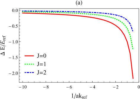
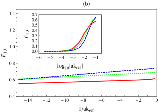
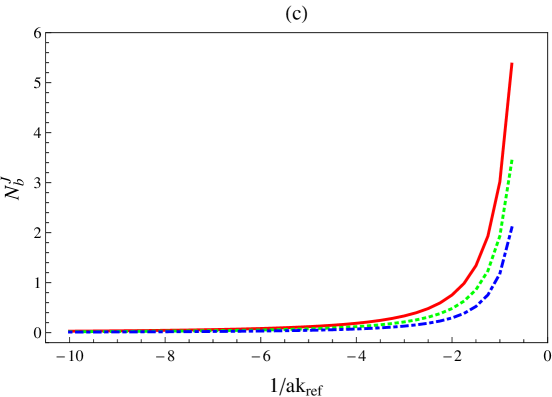
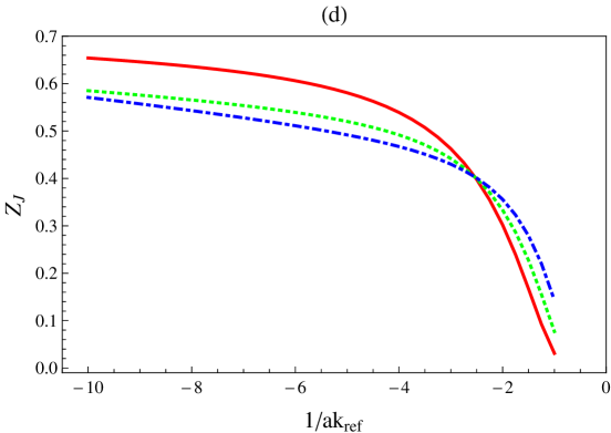
Figure 1: The energy shift (a), the variational parameter $F_{1J}$ (b), the total excited-boson number (c), and the quasi-particle residue (d) for $J=0,1,2$, as functions of the inverse of scattering length with the parameters in (43). The inset in the panel (b) is for smaller scattering-length region. The definitions of these quantities are given in (35), (27), (39), and (42), respectively.

The energy shift obtained here should be comparable with the experimental result Hu1 only for the case of small scattering lengths, roughly of $1/ak_{\rm ref}<-2$; it is because the Bogoliubov approximation (7) employed here works only if the number of excited bosons is less than or equal to the number of impurities, (it is the unity in the present calculation), and also the two-level approximation in the impurity wave function (27) is valid for the smaller values of variational solutions ($F_{1J}\ll F_{0J}$), and loses the validity when $F_{1J}\geq 1/\sqrt{2}\sim 0.7$. Also, the behavior of the residue implies that quasi-particle picture of the polaron works for about $1/ak_{\rm ref}<-2$ as well. In the case of the strong coupling regime and around the unitary limit, i.e., $|1/ak_{\rm ref}|<1$, we need to include effects of the two-to-two scattering processes between impurity and excited boson which were discarded in the Bogoliubov approximation; they are responsible for the effective in-medium shift in the unitary limit Shchadilova2 and the in-medium few-body bound states Levinsen2 ; Shchadilova2 .

V.2 Distributions of excited bosons

In Fig. 2 we show the solutions of variational parameter $f_{nl}$ for $J=0,1,2$, where we have set the impurity-boson scattering length by $a=-5.77{\rm nm}$ corresponding at $1/ak_{\rm ref}=-9.95$. The parameter $f_{nl}$ can be interpreted as the probability amplitude of excited bosons with the quantum numbers $(n,l)$.

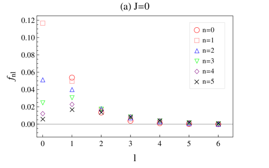
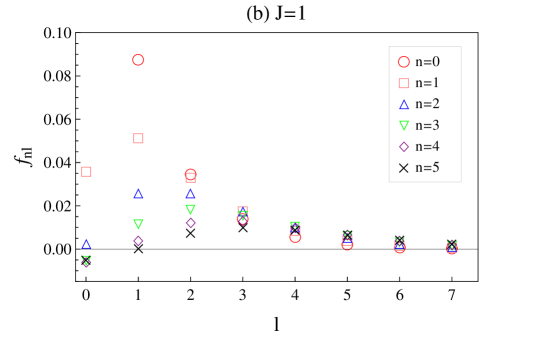
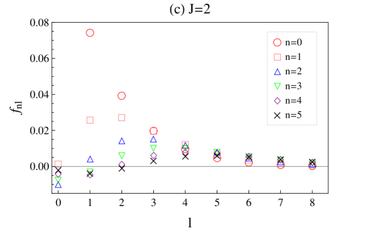
Figure 2: The variational parameter of excited bosons (31) for $J=0,1,2$ and their angular-momentum $l$-dependences. A set of parameters is given in (43), and $1/ak_{\rm ref}=-9.95$.

These figures implies that, for each principal quantum number $n$, the peak positions of $f_{nl}$ for the quantum number $l$ move to the right as the total angular momentum $J$ is increased. This is due to the attractive density-density-type interaction between impurity and bosons, which cause the large overlap between their wave functions to lower the interaction energy. It can be shown more directly in the real space distributions (Fig. 4-6).

In Fig. 3, we also show the quantum-number distributions of the excited bosons $N_{nlm}^{JJ_{z}}$ given by (38) for the states of $J=1,2$ as functions of the quantum number $m$ for $l=1,2,3$ and $n=0$, with the same parameter set as in Fig. 2.

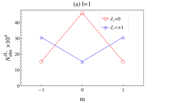
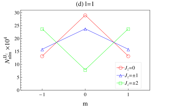
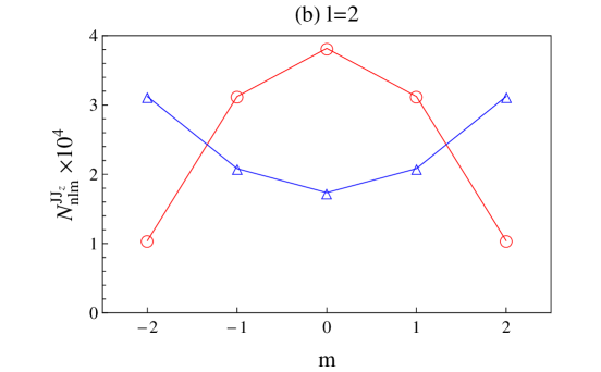
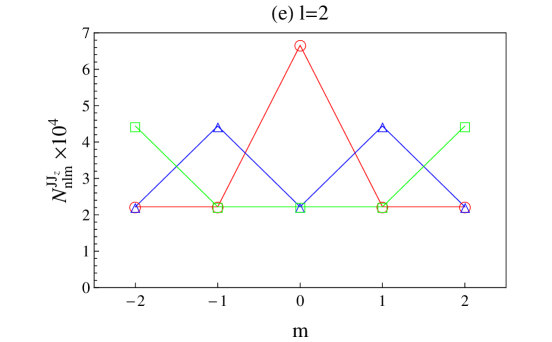
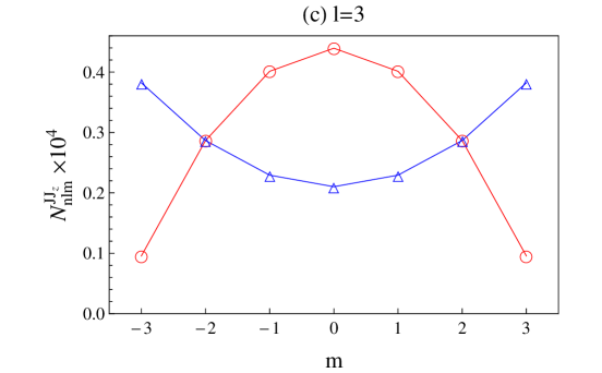
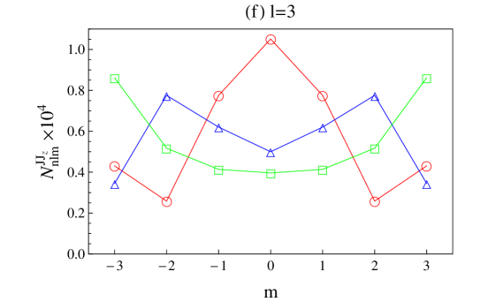
Figure 3: The angular-momentum $(l,m)$-dependences of the excited-boson numbers in (38) for $n=0$ and $l=1,2,3$. Panels (a), (b), (c) in left columns and (d), (e), (f) in right columns are for $J=1$ ($J_{z}=0,\pm 1$) and $J=2$ ($J_{z}=0,\pm 1,\pm 2$), respectively. The parameter set is the same as in Fig. 2.

As expected from the angular-momentum conservation and no drag effect, i.e., $\langle\hat{M}_{z}\rangle_{JJ_{z}}=0$, in the present calculation, all plots in the figures show that the distributions for the quantum number $m$ are symmetric about $m=0$. In order to understand the result, let’s suppose an impurity prepared in the state with a specific value of $J_{z}(=L_{z})$, which gives a specific direction in the space. If the interaction could be turned off between the impurity and surrounding bosons, the energy of the system should be still degenerate to the value of $J_{z}$. However, the presence of the real interaction causes the same number of virtual boson excitations with the quantum number $-|m|$ and $|m|$ in order to gain the interaction energy by a maximal overlap with the impurity (as shown in Fig. 4-6), which leads to the vanishing $\langle\hat{M}_{z}\rangle_{JJ_{z}}$.

For a different value of the principal quantum number $n\neq 0$, we have confirmed that the excited-boson number distributions have the completely same shape as that of $n=0$ since distribution shapes are determined by the Clebsch-Gordan coefficients for a given set of ($J,J_{z},l,m$), which are independent of $n$, but their intensities decrease with increasing $n$. The special case is for $J=J_{z}=0$, where the factor $N_{nlm}^{00}$ determined from the Clebsch-Gordan coefficients has no $m$ dependence; their numerical values for $l=1,2,3$ are $N_{01m}^{00}=9.76\times 10^{-4}$, $N_{02m}^{00}=0.38\times 10^{-4}$, and $N_{03m}^{00}=0.024\times 10^{-4}$, respectively.

Finally we show in Figs. 4-6 the real space distributions (40) of excited bosons together with impurity’s probability density obtained from (27) for the same parameter set as that in Fig. 2. To generate the distributions of excited bosons shown in Fig. 4-6, we have evaluated (40) in the approximation of taking quantum numbers up to $(n,l)=(5,5)$ in the summation, since $f_{nl}$ of higher quantum numbers does not contribute so much as the variational parameters (Fig. 2).

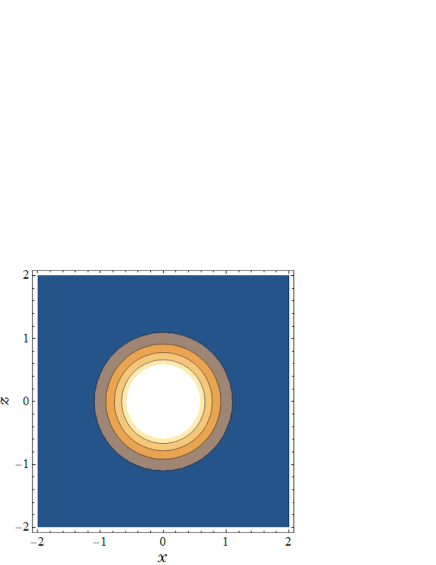
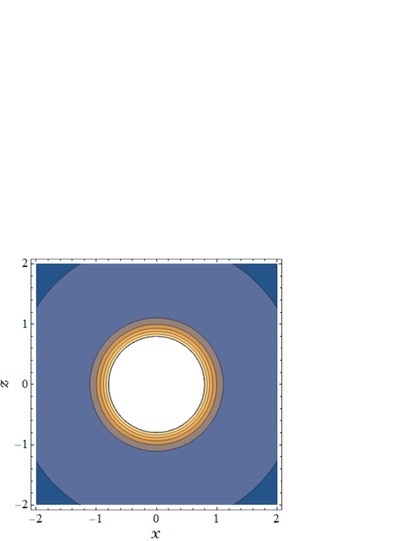
Figure 4: The $J=J_{z}=0$ contour plots of the impurity’s probability density $|\Psi_{JJ_{Z}}({\bf r})|^{2}$ (left panel) and the real-space excited-boson distributions (right panel) defined in (40), in the cross-section plane of $y=0$, where the ordinate is the $z$ axis (the direction of the magnetic quantum number), and the abscissa is the $x$ axis. Note that these plots have the rotational symmetry around the $z$ axis. The units of axes are $\left(\omega_{I}m_{I}\right)^{-1/2}$ (left) and $\left(\omega_{b}m_{b}\right)^{-1/2}$ (right), and the heights of the contour lines (not shown explicitly) are normalized by $\left(\omega_{I}m_{I}\right)^{3/2}$ (left) and $\left(\omega_{b}m_{b}\right)^{3/2}$ (right). The parameter set is the same as in Fig. 2.

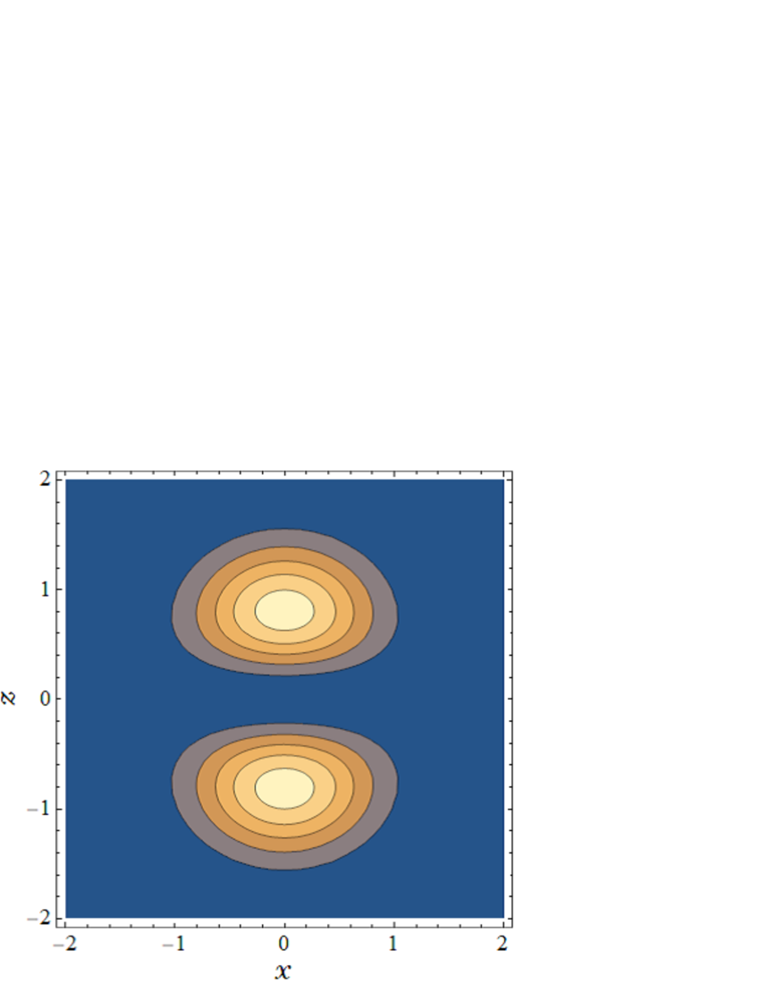
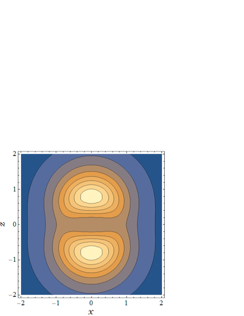
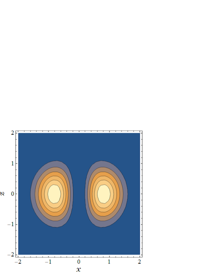
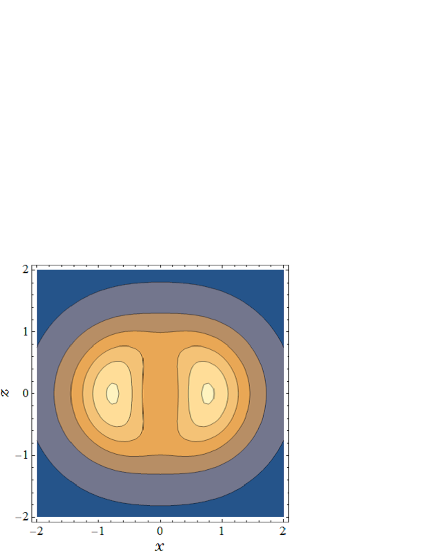
Figure 5: The $J=1$ contour plots of the impurity’s probability density (left panel) and the real-space excited-boson distributions (right panel): the top and bottom panels are for $|J_{z}|=0,1$. For other explanations, see the caption in Fig. 4.

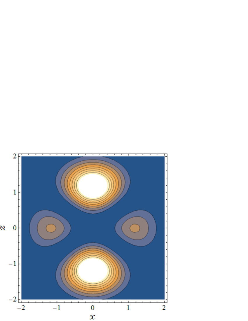
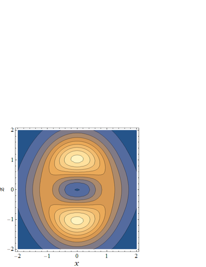
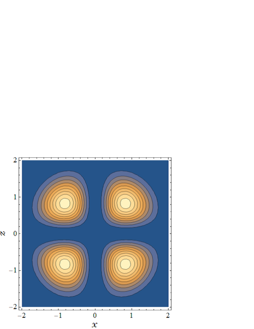
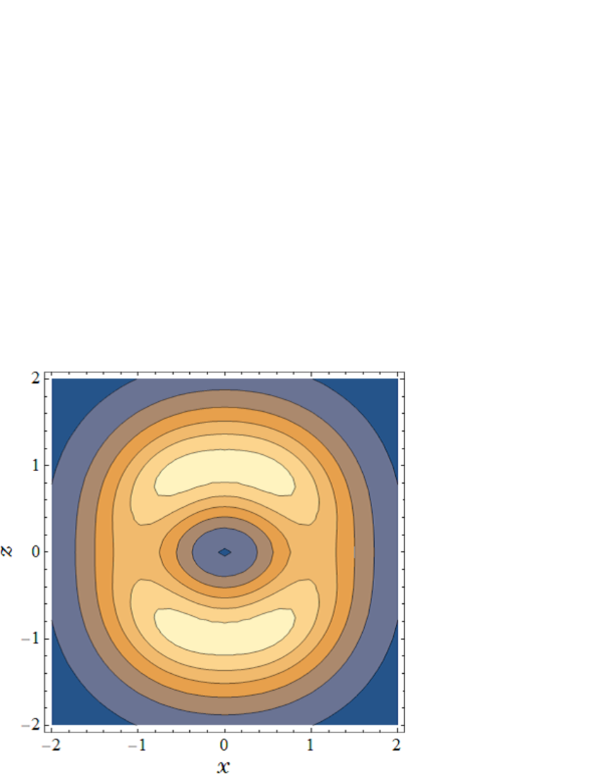
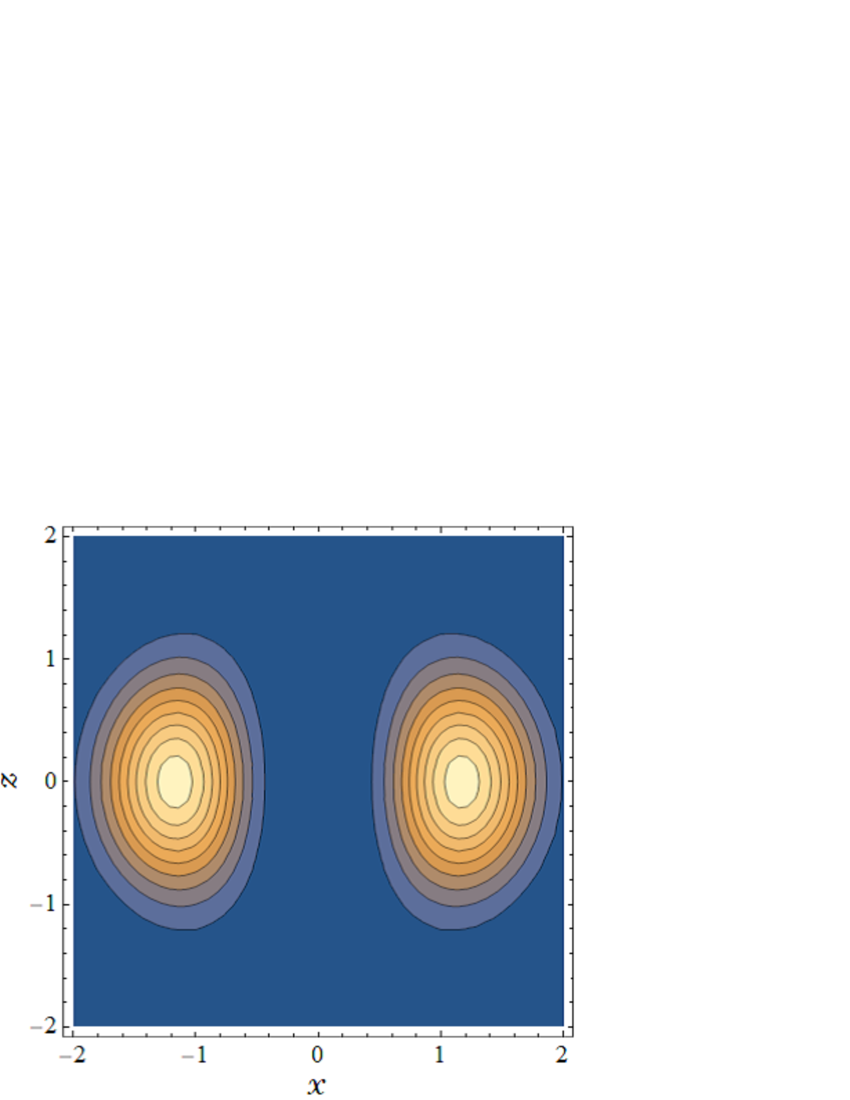
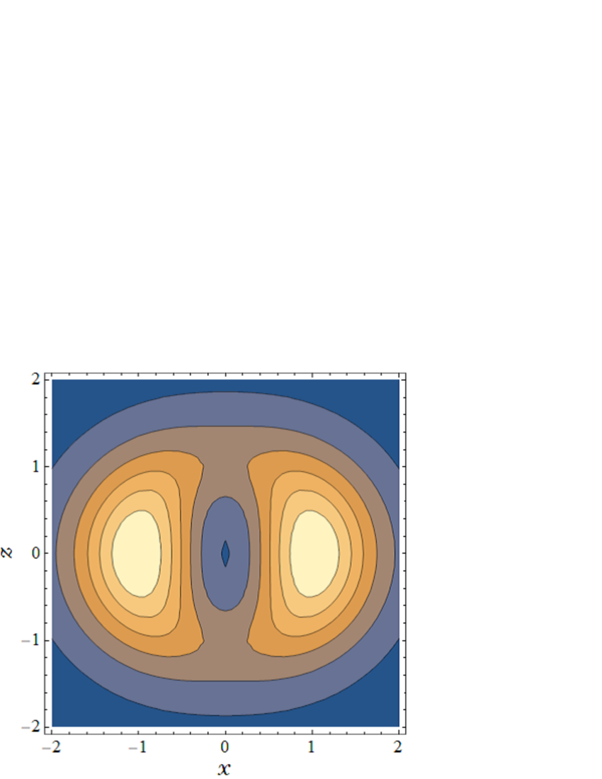
Figure 6: The $J=2$ contour plots of the impurity’s probability density (left panel) and the real-space excited-boson distributions (right panel): the top, middle, and bottom panels are for $|J_{z}|=0,1,2$. For other explanations, see the caption in Fig. 4.

Comparing left and right figures for $J=0,1,2$, we can observe that the attractive impurity-boson interaction has the effect that causes overlaps in their distributions, as discussed just above on the quantum-number distributions. The impurity’s probability is proportional to $|Y_{JJ_{z}}(\theta,\varphi)|^{2}$, thus the figures clearly exhibit the $s$, $p$, and $d$ orbital shapes for $J=0,1,2$, respectively. On the other hand, boson’s distributions are blurred because they always include $l=0$ isotropic contributions as shown in (40) with variationally-determined weight factor $|f_{nl}|^{2}$.

VI Summary and outlook

In this paper we have investigated the ground-state properties of the impurity interacting with medium-bosons in spherically symmetric trap potentials, when the total angular momentum $(J,J_{z})$ are given. To this end we have developed a conditional variational method, and obtained the ground-state energies, quasi-particle residue of polaron, and the quantum-number and real spaces distributions of excited bosons for the cases of total angular momenta $J=0,1,2$. From theoretical consideration, we have found that the expectation value $\langle\hat{J}^{2}\rangle_{JJ_{z}}=J(J+1)$ is shared by the impurity and the excited bosons as

$$\langle\hat{L}^{2}\rangle_{JJ_{z}} = J(J+1)+\sum^{\prime}_{n,l}l(l+1)|f_{nl}|^{2},$$

$$\langle\hat{M}^{2}\rangle_{JJ_{z}} = \sum^{\prime}_{n,l}l(l+1)|f_{nl}|^{2},$$

$$\langle 2\hat{L}\cdot\hat{M}\rangle_{JJ_{z}} = -2\sum^{\prime}_{n,l}l(l+1)|f_{nl}|^{2},$$ (46)

while that of the $z$-th component $\langle\hat{J}_{z}\rangle_{JJ_{z}}=J_{z}$ comes from the impurity only:

$$\langle\hat{L}_{z}\rangle_{JJ_{z}}=J_{z},\quad\langle\hat{M}_{z}\rangle_{JJ_{z}}=0,$$ (47)

which implies no drag effect for the polaron in the spherically-symmetric trap potentials. We have also made numerical calculations based on the variational method, and, as shown in Figs. 2-6, found that the excited bosons are distributed so as to make a large overlap with impurity’s probability density in real and quantum-number spaces because of the attractive impurity-boson interaction.

In the present study the excited bosons do not move collectively by themselves Dalfovo1 ; Japha1 since no boson-boson interaction is assumed, so they are in purely quantum regime. In most of recent experimental researches, the Bose polarons are realized in the system of the repulsive boson-boson interactions where the medium-bosons form a superfluid BEC. In order to analyze such cases, we need Bogoliubov-de-Gennes-type approaches Bogol1 ; Gennes1 ; Lewenstein4 ; Nakamura1 ; Nakamura2 ; Lampo1 beyond the Bogoliubov approximation. Such extensions of the present approach for the trapped polaron including the boson-boson interactions should give more detailed polaron’s structures such as a local depletion of BEC around impurity as well as the excitation spectra of the bosonic sector.

Finally, we comment a bit on the possibility of experimental observation of the finite angular momentum states of the trapped Bose polaron discussed in this paper. To our knowledge, all experiments have been done with axial-symmetric traps for both impurity and medium atoms, and no angular momentum is given to the atoms in total. To give some finite angular momentum to the system in axial symmetric trap potentials, we expect that the experimental methods of creating a vortex state of the BEC can be utilized Vor1 ; Vor2 : rotating a very dilute impurity-atom gas before switching on the interaction with medium bosons, and then the whole system, as Bose polaron, finally acquires some finite angular momentum. Furthermore, if the axial symmetric trap is deformed adiabatically to the spherical one, there remains the state with a finite angular momentum, the quantization axis of which should be the same with that of the original axial symmetry.

For the observation of the angular-momentum distribution of the impurity, the photon absorption spectra for excitations for the states with different angular momenta can be utilized, or the indirect observation of the phase of the impurity’s wave function, which has been done for the vortex state of the BEC Vor1 , is also an interesting possibility. At the moment, we have no fixed idea how to give a definite amount of angular momentum, but we think that a significant change in boson’s distribution can be observed with the methods as discussed here. Also, in the observation of the excited bosons, the photon absorption spectra mentioned above may work out for bosons as well. In addition, we think that in-situ experiments may also work to get images of excited bosons Yan8 ; insitu7 ; insitu8 ; insitu9 ; insitu10 ; insitu11 , although it would be a challenge since the total excited-boson number per impurity is quite small.

Acknowledgments

We are grateful to Kei Iida, Junichi Takahashi, and Ryosuke Imai for useful discussions on excitation spectra of interacting bosons in inhomogeneous systems, and to Kota Yanase for comments on angular momentum structure of excited nuclei. E. N. and H. Y. are supported by Grants-in-Aid for Scientific Research through Grants No. 17K05445 and No. 18K03501, respectively, provided by JSPS.

Appendix A Expectation values of operators by the coherent states

In this appendix we present the expectation values of the gauge-transformed operators $S^{-1}\hat{J}^{2}S$ and $S^{-1}{\mathcal{H}}S$, which are defined in (19) and (21), with respect to the coherent state (22). Using the expectation values of $\hat{M}_{i}$ and $\hat{L}_{i}$:

$$\left\langle\hat{M}_{i}\right\rangle_{b} = 0,$$ (48)

$$\left\langle\hat{M}_{\pm 1}\hat{M}_{\mp 1}\right\rangle_{b} = \Braket{l,0}{\hat{\mathcal{L}}_{\pm 1}\hat{\mathcal{L}}_{\mp 1}}{l,0}|f_{nl}|^{2}=-\frac{l(l+1)}{2}|f_{nl}|^{2},$$ (49)

and $\left\langle\hat{M}_{i}\hat{M}_{j}\right\rangle_{b}=0$ for the other combinations of $i$ and $j$, we obtain the expectation value of the shift operator:

$$\langle\hat{O}_{L}\rangle_{b} = \langle S^{-1}(\hat{L}^{2}S)\rangle_{b}$$ (50)

$$= \left\langle-\frac{\cot\theta}{\sqrt{2}}\left(\hat{M}_{-1}+\hat{M}_{+1}\right)-\frac{1}{2}\left(\hat{M}_{-1}+\hat{M}_{+1}\right)^{2}\right.$$

$$\qquad+\left.\frac{1}{\sin^{2}\theta}\left[\cos\theta\hat{M}_{0}-\sin\theta\frac{1}{\sqrt{2}}\left(\hat{M}_{-1}-\hat{M}_{+1}\right)\right]^{2}\right\rangle_{b}$$

$$= -\frac{1}{2}\left\langle\left(\hat{M}_{-1}+\hat{M}_{+1}\right)^{2}\right\rangle_{b}+\frac{1}{2}\left\langle\left(\hat{M}_{-1}-\hat{M}_{+1}\right)^{2}\right\rangle_{b}$$

$$= l(l+1)|f_{nl}|^{2}.$$

Then the expectation value of the transformed squared total angular momentum operators becomes

$$\left\langle S^{-1}\hat{J}^{2}S\right\rangle_{b} = \left\langle\hat{L}^{2}\right\rangle_{b}+\left\langle\hat{M}^{2}\right\rangle_{b}+\left\langle\hat{O}_{L}\right\rangle_{b}+2\sum_{i,j}D^{1}_{i,j}(\varphi,\theta,0)\left\langle\hat{M}_{j}^{\dagger}\left[S^{-1}(\hat{L}_{i}S)+\hat{L}_{i}\right]\right\rangle_{b}$$ (51)

$$= \hat{L}^{2}+l(l+1)|f_{nl}|^{2}+l(l+1)|f_{nl}|^{2}+2\sum_{i,j}D^{1}_{i,j}(\varphi,\theta,0)\left\langle\hat{M}_{j}^{\dagger}S^{-1}(\hat{L}_{i}S)\right\rangle_{b}$$

$$= \hat{L}^{2}+2l(l+1)|f_{nl}|^{2}-2\sum_{i=0,\pm 1}\Big{\{}D^{1}_{i,-1}(\varphi,\theta,0)\left\langle\hat{M}_{+1}S^{-1}(\hat{L}_{i}S)\right\rangle_{b}$$

$$\qquad\qquad\qquad\qquad\qquad\qquad\qquad+D^{1}_{i,+1}(\varphi,\theta,0)\left\langle\hat{M}_{-1}S^{-1}(\hat{L}_{i}S)\right\rangle_{b}\Big{\}}$$

$$= \hat{L}^{2},$$

Finally, we obtain the expectation value of the transformed Hamiltonian:

$$\langle S^{-1}{\mathcal{H}}S\rangle_{b} = H_{ho}({\bf r})+\frac{l(l+1)|f_{nl}|^{2}}{2m_{f}r^{2}}+E^{b}_{00}N_{0}+\sum_{n,l}^{\prime}E_{nl}^{b}|f_{nl}|^{2}+gN_{0}|\phi_{0}^{b}({\bf r})|^{2}$$ (52)

$$+g\frac{\sqrt{N_{0}}}{4\pi}\sum_{n,l}^{\prime}\sqrt{2l+1}R_{00}^{b}(r)R_{nl}^{b}(r)\left[f_{nl}+f^{*}_{nl}\right].$$

Appendix B The variational energy functional in terms of dimensionless variables

Here we present the coefficients appearing in the functionals (29) and (30). The functional $G[F_{0J};F_{1J}]$ is expanded as,

$$G[F_{0J};F_{1J}] := \int_{\bf r}\frac{1}{r^{2}}\left|\sum_{n=0,1}F_{nJ}\phi^{I}_{nJJ_{z}}({\bf r})\right|^{2}$$ (53)

$$= |F_{0J}|^{2}G^{0}_{J}+F_{0J}^{*}F_{1J}G^{c}_{J}+F_{1J}^{*}F_{0J}{G^{c}}^{*}_{J}+|F_{1J}|^{2}G^{1}_{J},$$

where the factors $G^{0}_{J}$, $G^{1}_{J}$, $G^{c}_{J}$ is given as $G^{0}_{J}=G^{1}_{J}=G^{c}_{J}\sqrt{J+\frac{3}{2}}=\frac{\omega_{I}m_{I}}{J+\frac{1}{2}}$.

The another functional $H[F_{0J};F_{1J}]_{nl}$ is represented as

$$H[F_{0J};F_{1J}]_{nl} := \int_{\bf r}R_{00}^{b}(r)R_{nl}^{b}(r)\left|\sum_{n=0,1}F_{nJ}\phi^{I}_{nJJ_{z}}({\bf r})\right|^{2}$$ (54)

$$= |F_{0J}|^{2}H_{nlJ}^{0}+F_{0J}^{*}F_{1J}H_{nlJ}^{c}+F_{1J}^{*}F_{0J}{H_{nlJ}^{c}}^{*}+|F_{1J}|^{2}H_{nlJ}^{1},$$

where

$$H_{nlJ}^{0} = \int_{0}^{\infty}{\rm d}rr^{2}R_{00}^{b}(r)R_{nl}^{b}(r)R^{I}_{0J}(r)^{2}$$ (55)

$$= \left(m_{I}\omega_{I}\right)^{\frac{3}{2}}{\mathcal{N}}_{00}{\mathcal{N}}_{nl}{\mathcal{N}}_{0J}^{2}Q^{2J}\int_{0}^{\infty}{\rm d}xx^{2+l+2J}\,e^{-\left(1+Q^{2}\right)x^{2}}L_{n}^{\left(\frac{1+2l}{2}\right)}\left(x^{2}\right)$$

$$= \left(m_{I}\omega_{I}\right)^{\frac{3}{2}}{\mathcal{N}}_{00}{\mathcal{N}}_{nl}{\mathcal{N}}_{0J}^{2}Q^{2J}(1+Q^{2})^{-\frac{3}{2}-J-\frac{l}{2}}\frac{\Gamma[\frac{3+2J+l}{2}]\Gamma[\frac{3+2l+2n}{2}]}{2\Gamma[\frac{3+2l}{2}]n!}$$

$$\qquad\times F\left(\frac{3+2J+l}{2},-n,\frac{3+2l}{2},\frac{1}{1+Q^{2}}\right),$$

$$H_{nlJ}^{c} = \int_{0}^{\infty}{\rm d}rr^{2}R_{00}^{b}(r)R_{nl}^{b}(r)R^{I}_{0J}(r)R^{I}_{1J}(r)$$

$$= \left(m_{I}\omega_{I}\right)^{\frac{3}{2}}{\mathcal{N}}_{00}{\mathcal{N}}_{nl}{\mathcal{N}}_{0J}{\mathcal{N}}_{1J}Q^{2J}$$

$$\qquad\times\int_{0}^{\infty}{\rm d}xx^{2+l+2J}\,e^{-\left(1+Q^{2}\right)x^{2}}L_{n}^{\left(\frac{1+2l}{2}\right)}\left(x^{2}\right)L_{1}^{\left(\frac{1+2J}{2}\right)}\left(Q^{2}x^{2}\right),$$

$$H_{nlJ}^{1} = \int_{0}^{\infty}{\rm d}rr^{2}R_{00}^{b}(r)R_{nl}^{b}(r)R^{I}_{1J}(r)^{2}$$ (57)

$$= \left(m_{I}\omega_{I}\right)^{\frac{3}{2}}{\mathcal{N}}_{00}{\mathcal{N}}_{nl}{\mathcal{N}}_{1J}^{2}Q^{2J}$$

$$\qquad\times\int_{0}^{\infty}{\rm d}xx^{2+l+2J}\,e^{-\left(1+Q^{2}\right)x^{2}}L_{n}^{\left(\frac{1+2l}{2}\right)}\left(x^{2}\right)\,\left\{L_{1}^{\left(\frac{1+2J}{2}\right)}\left(Q^{2}x^{2}\right)\right\}^{2},$$

where $Q=\sqrt{\frac{m_{I}\omega_{I}}{m_{b}\omega_{b}}}$. The $\Gamma(z)$ and $F(a,b,c,z)$ in the above formulas represent the gamma and Gauss’s hypergeometric functions, respectively. We have shown the analytic expression only for $H_{nlJ}^{0}$, but the remaining factors $H_{nlJ}^{c}$ and $H_{nlJ}^{1}$ also have similar analytic expressions, which are not presented here because they are lengthy and cumbersome.

In terms of dimensionless variables, the polaron binding energy (the energy shift (35) ), defined by the energy difference of the systems with and without the impurity-medium interaction is given by

$$\frac{\Delta E[F_{1J}]}{\omega_{b}} = 2\beta F_{1J}^{2}+\frac{N_{0}}{2}\left(1+\alpha\right)\alpha^{\frac{1}{2}}\beta^{\frac{3}{2}}\gamma\left[\tilde{H}_{00J}^{0}+2F_{1J}\sqrt{1-F_{1J}^{2}}\tilde{H}_{00J}^{c}+F_{1J}^{2}\left(\tilde{H}_{00J}^{1}-\tilde{H}_{00J}^{0}\right)\right]$$

$$-\frac{N_{0}}{4}\left(1+\alpha\right)^{2}\alpha\beta^{3}\gamma^{2}$$

$$\qquad\times\sum_{n,l}^{\prime}(2l+1)\frac{\left[\tilde{H}_{nlJ}^{0}+2F_{1J}\sqrt{1-F_{1J}^{2}}\tilde{H}_{nlJ}^{c}+F_{1J}^{2}\left(\tilde{H}_{nlJ}^{1}-\tilde{H}_{nlJ}^{0}\right)\right]^{2}}{\frac{3+2l+4n}{2}+\frac{l(l+1)}{2\left(J+\frac{1}{2}\right)}\beta\left[1+2F_{1J}\sqrt{1-F_{1J}^{2}}\left(J+\frac{3}{2}\right)^{-1/2}\right]},$$

$$= 2\beta F_{1J}^{2}-\frac{3\sqrt{N_{0}}}{2}\bar{f}_{00}[F_{1J}]$$

$$-\sum_{n,l}^{\prime}\bar{f}_{nl}[F_{1J}]^{2}\left[\frac{3+2l+4n}{2}+\frac{l(l+1)}{2J+1}\beta\left(1+2\frac{F_{1J}\sqrt{1-F_{1J}^{2}}}{\sqrt{J+\frac{3}{2}}}\right)\right],$$

where we have used the formal solution (31) :

$$\bar{f}_{nl}[F_{1J}] = -\frac{\sqrt{N_{0}}}{2}\left(1+\alpha\right)\alpha^{\frac{1}{2}}\beta^{\frac{3}{2}}\gamma$$ (59)

$$\times\sqrt{2l+1}\frac{\tilde{H}_{nlJ}^{0}+2F_{1J}\sqrt{1-F_{1J}^{2}}\tilde{H}_{nlJ}^{c}+F_{1J}^{2}\left(\tilde{H}_{nlJ}^{1}-\tilde{H}_{nlJ}^{0}\right)}{\frac{3+2l+4n}{2}+\frac{l(l+1)}{2\left(J+\frac{1}{2}\right)}\beta\left[1+2F_{1J}\sqrt{1-F_{1J}^{2}}\left(J+\frac{3}{2}\right)^{-1/2}\right]},$$

with $\tilde{H}_{nlJ}^{0}\equiv H_{nlJ}^{0}/(m_{I}\omega_{I})^{3/2}$ and so on, $\alpha\equiv m_{I}/m_{b}$, $\beta\equiv\omega_{I}/\omega_{b}$, and $\gamma\equiv a(m_{b}\omega_{b})^{1/2}$ via

$$\frac{g}{\omega_{b}}\left(m_{I}\omega_{I}\right)^{\frac{3}{2}} = \frac{2\pi a\left(m_{b}+m_{I}\right)}{m_{b}m_{I}}\frac{\left(m_{I}\omega_{I}\right)^{\frac{3}{2}}}{\omega_{b}}=2\pi\left(1+\frac{m_{I}}{m_{b}}\right)\frac{\omega_{I}}{\omega_{b}}a\left(m_{I}\omega_{I}\right)^{\frac{1}{2}}$$ (60)

$$= 2\pi\left(1+\frac{m_{I}}{m_{b}}\right)\left(\frac{m_{I}}{m_{b}}\right)^{\frac{1}{2}}\left(\frac{\omega_{I}}{\omega_{b}}\right)^{\frac{3}{2}}a\left(m_{b}\omega_{b}\right)^{\frac{1}{2}}$$

$$= 2\pi\left(1+\alpha\right)\alpha^{\frac{1}{2}}\beta^{\frac{3}{2}}\gamma.$$

Appendix C The ground-state energy in the second-order perturbation theory

In this appendix, we briefly show the derivation of the ground-state energy (37) obtained in the second-order perturbation theory. The Fröhlich-type Hamiltonian (1) in the full second-quantized form is represented as $\mathcal{H}=\mathcal{H}_{0}+\mathcal{V}$, where the non-perturbative and perturbative parts, $\mathcal{H}_{0}$ and $\mathcal{V}$ are defined as,

$$\mathcal{H}_{0} = \sum_{u}E_{u}^{I}a_{u}^{\dagger}a_{u}+E^{b}_{0}N_{0}+\sum_{s\neq 0}E_{s}^{b}b_{s}^{\dagger}b_{s},$$ (61)

$$\mathcal{V} = gN_{0}\sum_{u,u^{\prime}}C_{00;uu^{\prime}}a_{u}^{\dagger}a_{u^{\prime}}+g\sqrt{N_{0}}\sum_{s\neq 0,u,u^{\prime}}\left(C_{0s;uu^{\prime}}b_{s}+C_{s0;uu^{\prime}}b_{s}^{\dagger}\right)a_{u}^{\dagger}a_{u^{\prime}},$$ (62)

where $a_{u}$ ($a_{u}^{\dagger}$) is the annihilation (creation) operator of impurity with the labels of the abbreviated form $u=(n,l,m)$, and, also, the ground state is represented by $u=0$. The overlap integrals $C_{ss^{\prime};uu^{\prime}}$ of the wave functions are defined by

$$C_{ss^{\prime};uu^{\prime}}=\int_{{\bf r}}{\phi^{b}_{s}}^{*}({\bf r})\phi^{b}_{s^{\prime}}({\bf r}){\phi^{I}_{u}}^{*}({\bf r})\phi^{I}_{u^{\prime}}({\bf r}).$$ (63)

In the diagrammatic method of the perturbation theory, the ground state energy is obtained from the summation of the connected diagrams (Goldstone’s theorem). Up to the second order of $g$ for $J=J_{z}=0$, it becomes

$$\braket{\mathcal{H}} = \braket{\Phi_{0}}{\mathcal{H}_{0}}{\Phi_{0}}+\braket{\Phi_{0}}{\mathcal{V}}{\Phi_{0}}+\sum_{i}\frac{\braket{\Phi_{0}}{\mathcal{V}}{i}\braket{i}{\mathcal{V}}{\Phi_{0}}}{\braket{\Phi_{0}}{\mathcal{H}_{0}}{\Phi_{0}}-\braket{i}{\mathcal{H}_{0}}{i}}$$

$$= E_{0}^{f}+E_{0}^{b}N_{0}+gN_{0}C_{00;00}$$

$$+\sum_{s\neq 0,u}\frac{\left|\braket{0}{b_{s}a_{u}\mathcal{V}a_{0}^{\dagger}}{0}\right|^{2}}{E_{0}^{I}+E_{0}^{b}N_{0}-\braket{0}{b_{s}a_{u}\left(\sum_{u^{\prime}}E_{u^{\prime}}^{I}a_{u^{\prime}}^{\dagger}a_{u^{\prime}}+E^{b}_{0}N_{0}+\sum^{\prime}_{s^{\prime}}E_{s^{\prime}}^{b}b_{s^{\prime}}^{\dagger}b_{s^{\prime}}\right)a_{u}^{\dagger}b_{s}^{\dagger}}{0}}$$

$$+\sum_{u\neq 0}\frac{\left|\braket{0}{a_{u}\mathcal{V}a_{0}^{\dagger}}{0}\right|^{2}}{E_{0}^{I}+E_{0}^{b}N_{0}-\braket{0}{a_{u}\left(\sum_{u^{\prime}}E_{u^{\prime}}^{I}a_{u^{\prime}}^{\dagger}a_{u^{\prime}}+E^{b}_{0}N_{0}+\sum^{\prime}_{s^{\prime}}E_{s^{\prime}}^{b}b_{s^{\prime}}^{\dagger}b_{s^{\prime}}\right)a_{u}^{\dagger}}{0}}$$

$$= E_{0}^{I}+E_{0}^{b}N_{0}+gN_{0}C_{00;00}-g^{2}N_{0}\sum_{s\neq 0,u}\frac{C_{0s;0u}C_{s0;u0}}{E_{u}^{I}-E_{0}^{I}+E_{s}^{b}}-g^{2}N_{0}^{2}\sum_{u\neq 0}\frac{C_{00;0u}C_{00;u0}}{E_{u}^{I}-E_{0}^{I}},$$

where the non-perturbative ground state are defined by

$$\ket{\Phi_{0}} = a_{0}^{\dagger}\ket{0}$$ (65)

with the Fock vacuum of excited bosons $\ket{0}$ (the condensed state of the lowest-energy boson), and the intermediate states $\ket{i}$ are

$$\ket{i} = \left\{a_{u}^{\dagger}b_{s\neq 0}^{\dagger}\ket{0},\,a_{u\neq 0}^{\dagger}\ket{0}\right\}.$$ (66)

In order to make a fair comparison with the variational method, in the ground-state energy formula ($J=0$) , we take the impurity intermediate states up to $u=(1,0,0)$, and those of bosons only for $l=m=0$ (consistent with the $J=0$ state). Then we obtain the ground-state energy in the second-order perturbation theory:

$$\braket{\mathcal{H}} \simeq E_{00}^{I}+E_{00}^{b}N_{0}+g\frac{N_{0}}{4\pi}H_{000}^{0}$$

$$- g^{2}\frac{N_{0}}{\left(4\pi\right)^{2}}\sum_{n\neq 0}\left(\frac{|H_{n00}^{c}|^{2}}{E_{10}^{I}-E_{00}^{I}+E_{n0}^{b}}+\frac{|H_{n00}^{0}|^{2}}{E_{n0}^{b}}\right)-g^{2}\left(\frac{N_{0}}{4\pi}\right)^{2}\frac{|H_{000}^{c}|^{2}}{E_{10}^{I}-E_{00}^{I}},$$

which is just the eq.  (37).

References

- (1) J. Catani, G. Lamporesi, D. Naik, M. Gring, M. Inguscio, F. Minardi, A. Kantian, and T. Giamarchi, Phys. Rev. A 85, 023623 (2012).
- (2) R. Scelle, T. Rentrop, A. Trautmann, T. Schuster, and M. K. Oberthaler, Phys. Rev. Lett. 111, 070401 (2013).
- (3) M. Hohmann, F. Kindermann, B. Gänger, T. Lausch, D. Mayer, F. Schmidt and A. Widera, EPJ Quantum Technology 2:23, (2015)
- (4) E. Compagno, G. De Chiara, D. G. Angelakis, and G. M. Palma, Scientific Reports vol. 7, 2355 (2017).
- (5) N. B. Jørgensen, L. Wacker, K. T. Skalmstang, M. M. Parish, J. Levinsen, R. S. Christensen, G. M. Bruun, J. J. Arlt, Phys. Rev. Lett. 117, 055302 (2016).
- (6) M. -G. Hu, M. J. Van de Graaff, D. Kedar, J. P. Corson, E. A. Cornell, and D. S. Jin, Phys. Rev. Lett. 117, 055301 (2016).
- (7) T. Rentrop, A. Trautmann, F. A. Olivares, F. Jendrzejewski, A. Komnik, and M. K. Oberthaler, Phys. Rev. X 6, 041041 (2016).
- (8) B. Fröhlich, M. Feld, E. Vogt, M. Koschorreck, W. Zwerger, and M. Köhl, Phys. Rev. Lett. 106, 105301 (2011).
- (9) F. Scazza, G. Valtolina, P. Massignan, A. Recati, A. Amico, A. Burchianti, C. Fort, M. Inguscio, M. Zaccanti, and G. Roati, Phys. Rev. Lett. 118, 083602 (2017).
- (10) M. Cetina, M. Jag, R. S. Lous, I. Fritsche, J. T. M. Walraven, R. Grimm, J. Levinsen, M. M. Parish, R. Schmidt, M. Knap, and E. Demler, Science 354, 96 (2016).
- (11) C. J. Pethick and H. Smith, Bose-Einstein Condensation in Dilute Gases (Cambridge University Press, Cambridge, 2008).
- (12) L. Pitaevskii and S. Stringari, Bose-Einstein Condensation (Oxford, New York, 2003).
- (13) F. M. Cucchietti and E. Timmermans, Phys. Rev. Lett. 96, 210401 (2006).
- (14) K. Sacha and E. Timmermans, Phys. Rev. A 73, 063604 (2006).
- (15) J. Tempere, W. Casteels, M. K. Oberthaler, S. Knoop, E. Timmermans, and J. T. Devreese, Phys. Rev. B 80, 184504 (2009).
- (16) W. Casteels, T. Van Cauteren, J. Tempere, and J. T. Devreese, Laser Physics 21, 8, pp 1480-1485 (2011).
- (17) S. P. Rath and R. Schmidt, Phys. Rev. A, 88, 053632 (2013)
- (18) A. Shashi, F. Grusdt, D. A. Abanin, and E. Demler, Phys. Rev. A 89, 053617 (2014).
- (19) W. Li and S. Das Sarma, Phys. Rev. A 90, 013618 (2014).
- (20) J. Levinsen, M. M. Parish, and G. M. Bruun, Phys. Rev. Lett. 115, 125302 (2015).
- (21) A. S. Dehkharghani, A. G. Volosniev, and N. T. Zinner, Phys. Rev. A 92, 031601(R) (2015).
- (22) L. A. Peña Ardila and S. Giorgini, Phys. Rev. A 92, 033612 (2015).
- (23) R. S. Christensen, J. Levinsen, and G. M. Bruun, Phys. Rev. Lett. 115, 160401 (2015)
- (24) J. Vlietinck, W. Casteels, K. Van Houcke, J. Tempere, J. Ryckebusch, and J. T. Devreese, New J. Phys. 17,033023 (2015).
- (25) F. Grusdt, Y. E. Shchadilova, A. N. Rubtsov, and E. Demler, Sci. Rep. 5, 12124 (2015).
- (26) F. Grusdt and M. Fleischhauer, Phys. Rev. Lett. 116, 053602 (2016).
- (27) Y. E. Shchadilova, F. Grusdt, A. N. Rubtsov, and E. Demler, Phys. Rev. A 93, 043606 (2016)
- (28) Y. E. Shchadilova, R. Schmidt, F. Grusdt, and E. Demler, Phys. Rev. Lett. 117, 113002 (2016).
- (29) F. Grusdt, K. Seetharam, Y. Shchadilova, and E. Demler, Phys. Rev. A 97, 033612 (2018).
- (30) Y. Ashida, R. Schmidt, L. Tarruell, and E. Demler Phys. Rev. B 97, 060302(R) (2018).
- (31) L. A. Peña Ardila, N. B. Jørgensen, T. Pohl, S. Giorgini, G. M. Bruun, and J. J. Arlt, arXiv:1812.04609.
- (32) K. K. Nielsen, L. A. Peña Ardila, G. M. Bruun, and T. Pohl, arXiv:1806.09933.
- (33) Effective One-Body Approach to Impurities in One-Dimensional Trapped Bose Gases, S. I. Mistakidis, A. G. Volosniev, N. T. Zinner, P. Schmelcher , arXiv:1809.01889
- (34) Quench Dynamics and Orthogonality Catastrophe of Bose Polarons, S. I. Mistakidis, G. C. Katsimiga, G. M. Koutentakis, Th. Busch, P. Schmelcher, arXiv:1811.10702
- (35) See, for instance, A. S. Alexandrov, J. T. Devreese, Advances in Polaron Physics, Springer Series in Solid-State Sciences Vol. 159, (Springer, 2009).
- (36) L. D. Landau, Phys. Z. Sowjetunion 3, 664 (1933); L. Landau and S. Pekar, J. Exptl. Theor. Phys. 18, 419 (1948); S. Pekar, J. Exptl. Theor. Phys. 19, 796 (1949).
- (37) H. Fröhlich, Theory of Dielectrics, (Clarendon Press, Oxford, 1949); H. Fröhlich, H. Pelzer, and S. Zienau, Phil. Mag. 41, 221 (1950); H. Fröhlich, Adv. Phys. 3, 325 (1954).
- (38) F. Chevy, Phys. Rev. A 74, 063628 (2006); Unitary polarized Fermi gases, p. 607 in Ultra-Cold Fermi Gases, Eds. M. Inguscio, W. Ketterle, C. Salomon, (IOS Press, Amsterdam, 2007).
- (39) P. Massignan, G. M. Bruun, and H. T. C. Stoof Phys. Rev. A 78, 031602(R) (2008).
- (40) A. Schirotzek, C. -H. Wu, A. Sommer, and M. W. Zwierlein, Phys. Rev. Lett. 102, 230402 (2009).
- (41) M. Ku, J. Braun, and A. Schwenk, Phys. Rev. Lett. 102, 255301 (2009).
- (42) R. Schmidt and T. Enss, Phys. Rev. A 83, 063620 (2011).
- (43) C. Kohstall, M. Zaccanti, M. Jag, A. Trenkwalder, P. Massignan, G. M. Bruun, F. Schreck, and R. Grimm, Nature 485, 615-618 (2012).
- (44) M. Koschorreck, D. Pertot, E. Vogt, B. Fröhlich, M. Feld, and M. Köhl, Nature 485, 619 (2012).
- (45) R. Schmidt, T. Enss, V. Pietilä, and E. Demler, Phys. Rev. A 85, 021602(R) (2012).
- (46) J. Vlietinck, J. Ryckebusch, and K. Van Houcke, Phys. Rev. B 87, 115133 (2013).
- (47) C. Trefzger and Y. Castin, Europhysics Letters 104, 50005 (2013).
- (48) C. Trefzger and Y. Castin, Phys. Rev. A 90, 033619 (2014).
- (49) P. Massignan, M. Zaccanti, and G. M. Bruun, Reports on Progress in Physics, 77, 034401, (2014).
- (50) Z. Lan and C. Lobo, J. Indian Inst. Sci.—94, 179 (2014)
- (51) Z. Lan and C. Lobo, Phys. Rev. A 92, 053605 (2015)
- (52) F. N. Ünal, B. Hetényi, and M. Ö. Oktel, Phys. Rev. A 91, 053625 (2015).
- (53) W. Yi and X. Cui Phys. Rev. A 92, 013620 (2015).
- (54) M. M. Parish and J. Levinsen, Phys. Rev. B 94, 184303 (2016).
- (55) J. Levinsen, P. Massignan, S. Endo, M. M. Parish, J. Phys. B: At. Mol. Opt. Phys. 50, 072001 (2017).
- (56) K. Kamikado, T. Kanazawa, and S. Uchino, Phys. Rev. A 95, 013612 (2017).
- (57) B. Kain and H. Y. Ling, Phys. Rev. A 96, 033627 (2017)
- (58) R. Schmidt, M. Knap, D. A. Ivanov, J.-S. You, M. Cetina, E. Demler, Rep. Prog. Phys. 81, 024401 (2018).
- (59) Repulsive Fermi Polarons and Their Induced Interactions in Binary Mixtures of Ultracold Atoms, S. I. Mistakidis, G. C. Katsimiga, G. M. Koutentakis, P. Schmelcher, arXiv:1808.00040.
- (60) J. Levinsen, P. Massignan, F. Chevy, and C. Lobo, Phys. Rev. Lett. 109, 075302 (2012).
- (61) T. -S. Deng, Z. -C. Lu, Y. -R. Shi, J. -G. Chen, W. Zhang, and W. Yi, Phys. Rev. A 97, 013635 (2018).
- (62) B. Kain and H. Y. Ling, Phys. Rev. A 89, 023612 (2014).
- (63) Ground-state properties of Dipolar Bose polarons, L. A. Peña Ardila and T. Pohl, arXiv:1804.06390
- (64) H. Tajima and S. Uchino, New J. Phys. 20, 073048 (2018).
- (65) Boiling a Unitary Fermi Liquid, Z. Yan, P. B. Patel, B. Mukherjee, R. J. Fletcher, J. Struck, and M. W. Zwierlein, arXiv:1811.00481
- (66) Thermal crossover, transition, and coexistence in Fermi polaronic spectroscopies, H. Tajima and S. Uchino, arXiv:1812.05889
- (67) J. Levinsen, M. M. Parish, R. S. Christensen, J. J. Arlt, and G. M. Bruun, Phys. Rev.—A 96, 063622 (2017).
- (68) N.-E. Guenther, P. Massignan, M. Lewenstein, and G. M. Bruun, Phys. Rev. Lett.120, 050405 (2018).
- (69) M. Bruderer, Alexander Klein, Stephen R. Clark, and Dieter Jaksch, Phys. Rev. A 76(R):011605 (2007); New J. Phys. 10, 033015 (2008).
- (70) E. Nakano and H. Yabu, Phys. Rev. B 93, 205144 (2016).
- (71) For instance, see, David J. Rowe, Nuclear collective motion : models and theory (World Scientific, New Jersey, 2010)
- (72) D. R. Inglis, Phys. Rev. 96, 1059 (1954) ; 96, 701 (1955).
- (73) D. J. Thouless and J. G. Valatin, Nucl. Phys. 31, 211-230 (1962).
- (74) R. Schmidt and M. Lemeshko, Phys. Rev. Lett. 114, 203001 (2015).
- (75) R. Schmidt and M. Lemeshko, Phys. Rev. X 6, 011012 (2016).
- (76) E. Yakaboylu, B. Midya, A. Deuchert, N. Leopold, and M. Lemeshko Phys. Rev. B 98, 224506 (2018).
- (77) E. Nakano, H. Yabu, and K. Iida, Phys. Rev. A 95, 023626 (2017)
- (78) M. E. Rose, Elementary Theory of Angular Momentum (Dover Publications, 2011).
- (79) A. R. Edmonds, Angular Momentum in quantum mechanics (Princeton University Press, New Jersey, 1957).
- (80) T. D. Lee, F. E. Low, and D. Pines, Phys. Rev. 90, No.2, 297-302 (1953).
- (81) S. S. Schweber, An Introduction to Relativistic Quantum Field Theory, (Dover Publications, New York, 2005).
- (82) F. Dalfovo, S. Giorgini, L. P. Pitaevskii, and S. Stringari, Rev. Mod. Phys. 71, 463 (1999).
- (83) Y. Japha and Y. B. Band, Phys. Rev. A 84, 033630 (2011).
- (84) N. N. Bogoliubov, J. Phys. (Moscow) 11, 32 (1947).
- (85) P. G. de Gennes, Superconductivity of Metals and Alloys (Benjamin, New York, 1966).
- (86) M. Lewenstein and L. You, Phys. Rev. Lett. 77, 3489 (1996).
- (87) Y. Nakamura, J. Takahashi, and Y. Yamanaka, Phys. Rev. A 89 013613 (2014).
- (88) Y. Nakamura, T. Kawaguchi, Y. Torii, and Y. Yamanaka, Annals of Physics 376, 484 (2017).
- (89) A. Lampo, C. Charalambous, M. A. Garcia-March, and M. Lewenstein, arXiv:1803.08946.
- (90) M. R. Matthews, B. P. Anderson, P. C. Haljan, D. S. Hall, C. E. Wieman, and E. A. Cornell, Phys. Rev. Lett. 83, 2498 (1999).
- (91) K. W. Madison, F. Chevy, W. Wohlleben, and J. Dalibard, Phys. Rev. Lett. 84, 806 (2000); J. R. Abo-Shaeer, C. Raman, J. M. Vogels, W. Ketterle, Science 292, 476 (2001).
- (92) Y. -I. Shin, C. H. Schunck, A. Schirotzek, and W. Ketterle, Nature 451, 689-693 (2008).
- (93) W. S. Bakr, J. I. Gillen, A. Peng, S. Fölling, and M. Greiner, Nature 462, 74-77 (2009).
- (94) J. F. Sherson, C. Weitenberg, M. Endres, M. Cheneau, I. Bloch, and S. Kuhr, Nature 467, 68-72 (2010).
- (95) M. Horikoshi, S. Nakajima, M. Ueda, and T. Mukaiyama, Science 327, 442 (2010).
- (96) M. J. H. Ku, A. T. Sommer, L. W. Cheuk, and M. W. Zwierlein, Science 335, 563 (2012).