Abstract

We classify all Kutasov-Seiberg type dualities in large $N_{c}$ SQCD with adjoints of rational $R$-charges. This is done by equating the superconformal index of the electric and magnetic theories: the obtained equation has a solution each time some product of cyclotomic polynomials has only positive coefficients. In this way we easily reproduce without any reference to the superpotential or the choice of the equations of motion (classical chiral ring) all the known dualities from the literature, while adding to them a new family with two adjoints with $R$ charges $\frac{2}{2k+1}$ and $\frac{2(k+1)}{2k+1}$ for all integers $k>1$. We argue that these new fixed points could be in their appropriate conformal windows and in some range of the Yukawas involved a low energy limit of the $D_{2k+2}$ fixed point. We try to clarify some issues connected to the difference between classical and quantum chiral ring of this new solution.

1 Introduction

There are many known candidates for IR fixed points in SQCD with $N_{A}$ adjoints connected with a free theory in the UV: they are described for no ($N_{A}=0$) adjoints in [1], for $N_{A}=1$ adjoint in [2, 3, 4], and $N_{A}=2$ adjoints in [7]. Larger values of $N_{A}>2$ are unavailable for branches of the flows which end up eventually into a free UV fixed point. Several of the above fixed points have, in a specified conformal window, a known candidate for a non-trivial dual: [1] in the case $N_{A}=0$, [8] for $N_{A}=1$, while for $N_{A}=2$ the known duals are for $D_{k+2}$ [5, 6, 7] and $E_{7}$ [9, 10].

In this paper we will try to derive in a different way these fixed points of SQCD with adjoints with known duals. We will assume that the $R$-charges of the adjoints are rational numbers, as if determined from a marginal superpotential. We will show that with such an assumption a complete (although in principle infinite) classification of all solutions with valid duality through the equality of the superconformal index [13, 14, 15] at large $N_{c}$ [16] can be found. This is because, as we will see, such an equality can be written as a factorisation of a polynomial $y^{n}-1$ for integer $n>1$ into a product of a polynomial with only non-negative integer coefficients (representing the contribution of the mesons) with a specific (antipalindromic) polynomial (representing the contributions of all the gauge adjoints of the theory) to be specified later on. It is well known that every polynomial of the form $y^{n}-1$ for a fixed integer $n$ can be written as a unique product of so-called cyclotomic polynomials [17]. Our classification of all duals is thus transformed into a classification of all products of distinct cyclotomic polynomials with only non-negative coefficients. Although we were unable to find an explicit analytic classification of this mathematical problem, the formulation helps in finding the solutions: choose $n>1$, find the factorisation of $y^{n}-1$ into product of cyclotomic polynomials, and find all the partial products which end up into polynomials with non-negative coefficients.

With such a recipe we can easily reproduce the known dualities in the case of $N_{A}\leq 2$, i.e. SQCD, $A_{k}$, $D_{k+2}$ and $E_{7}$. We can however find out other possible rational solutions for $R$-charges between $0$ and $2$, which we were unable to locate in the existing literature. We will mention here the family with $N_{A}=2$ and the adjoint $R$-charges $\frac{2}{2k+1}$ and $\frac{2(k+1)}{2k+1}$ for integer $k>1$. Although it is easy to write down a superpotential which, when marginal, produces such $R$-charges, the classical determination of the mesons needed in the dual theory using the equations of motion seems incomplete. On the other side using the equality of the superconformal indices the mesons’ $R$-charges and thus their structure come out automatically as an output. We will show how this comes about in the quantum chiral ring from the explicit evaluation of few low order terms of the superconformal index. We found also a possible interpretations for such new fixed points: they could be IR limits of the $D_{2k+2}$ fixed point, perturbed by a relevant operator in a specified conformal window.

We will first give in section 2 a short summary from the literature of the calculation of the superconformal index and its use in comparing dual theories at large $N_{c}$. We will use it to derive the main equation, i.e. eq. (2.17) for SQCD with $N_{A}$ adjoints. In the following section 3 we will then show how to go through the ordered but infinite solutions of the main equation (2.17), by using the notion of cyclotomic polynomials. Here we will also describe some old and new solutions from our new way of classifying them. In section 4 we will take some time to interpret the new solution found, i.e. in which flow it may appear, and check its quantum chiral ring from the superconformal index. We will then conclude in section 5 and add three appendices.

2 The superconformal index

We first summarise the computation of the superconformal index (for a nice review see for example [18]) following mainly [15, 16, 19].

The first step is to calculate the index over the single particle states through

$$i(t,x,z,y)=\frac{2t^{2}-t(x+x^{-1})}{(1-tx)(1-tx^{-1})}\chi_{adj}(z)+\sum_{j}\frac{t^{R_{J}}\chi_{F(j)}(y)\chi_{G(j)}(z)-t^{2-R_{j}}\chi_{\bar{F}(j)}(y)\chi_{\bar{G}(j)}(z)}{(1-tx)(1-tx^{-1})}$$ (2.1)

where $t$, $x$, $z$, $y$ are fugacities (chemical potentials) defined for the generators of conserved quantities in the theory considered: $t$ and $x$ for the superconformal group on $R\times S^{3}$ where the index is defined, while $z$ and $y$ are for the gauge and global symmetry groups, respectively. $\chi$ is the group character which is in SU(N)

$$\chi_{fundamental}(u)=p_{N}(u)\equiv\sum_{i=1}^{N}u_{i} \chi_{antifundamental}(u)=p_{N}(u^{-1})$$ , (2.2)

$$\chi_{adjoint}(u)=p_{N}(u)p_{N}(u^{-1})-1 \chi_{singlet}=1$$ , (2.3)

and $\prod_{i=1}^{N}u_{i}=1$.

In (2.1) the first term is the contribution of the gauge fields, while $j$ in the sum of the second term runs over all the chiral superfields: the term proportional to $t^{R_{j}}$ is the contribution of the boson $\phi_{j}$ with $R$-charge $R_{j}$ while the term proportional to $t^{2-R_{j}}$ is the contribution of the fermion $\bar{\psi}_{j}$. Notice that $\psi_{j}$ is the superpartner of $\phi_{j}$. $F(j)$ and $G(j)$ stand for the representations of the flavour and gauge group respectively of the chiral superfield $j$.

Now it is easy to write the index for our specific case of $N_{A}$ adjoints with R charges $R_{i}$ and $N_{f}$ pairs of vectorlike quarks $Q+\tilde{Q}$:

$$i(t,x,y,\tilde{y},v,z) = \frac{2t^{2}-t(x+x^{-1})+\sum_{a=1}^{N_{A}}(t^{R_{a}}-t^{2-R_{a}})}{(1-tx)(1-tx^{-1})}\left(p_{N}(z)p_{N}(z^{-1})-1\right)$$ (2.4)

$$+ \frac{\left(t^{R_{Q}}p_{N_{f}}(y)-t^{2-R_{Q}}p_{N_{f}}(\tilde{y})\right)v}{(1-tx)(1-tx^{-1})}p_{N}(z)$$

$$+ \frac{\left(t^{R_{Q}}p_{N_{f}}(\tilde{y}^{-1})-t^{2-R_{Q}}p_{N_{f}}(y^{-1})\right)v^{-1}}{(1-tx)(1-tx^{-1})}p_{N}(z^{-1})$$

where instead of a single $y$ we used $y$ itself for the group SU($N_{f}$)_Q, $\tilde{y}$ for SU($N_{f}$)${}_{\tilde{Q}}$, and $v$ for the baryonic U(1)_B.

In short we can thus write

$$i(w,z)=f(w)\left(p_{N}(z)p_{N}(z^{-1})-1\right)+g(w)p_{N}(z)+\bar{g}(w)p_{N}(z^{-1})+h(w)$$ (2.5)

where we denoted by $w$ all the fugacities except the gauge $z$ (i.e. in our case $t,x,y,\tilde{y},v$).

For the electric theory we are considering

$$f_{E} = \frac{2t^{2}-t(x+x^{-1})+\sum_{a=1}^{N_{A}}(t^{R_{a}}-t^{2-R_{a}})}{(1-tx)(1-tx^{-1})}$$ (2.6)

$$g_{E} = \frac{\left(t^{R_{Q}}p_{N_{f}}(y)-t^{2-R_{Q}}p_{N_{f}}(\tilde{y})\right)v}{(1-tx)(1-tx^{-1})}$$ (2.7)

$$\bar{g}_{E} = \frac{\left(t^{R_{Q}}p_{N_{f}}(\tilde{y}^{-1})-t^{2-R_{Q}}p_{N_{f}}(y^{-1})\right)v^{-1}}{(1-tx)(1-tx^{-1})}$$ (2.8)

$$h_{E} = 0$$ (2.9)

while the magnetic theory of Seiberg type has

$$f_{M} = \frac{2t^{2}-t(x+x^{-1})+\sum_{a=1}^{N_{A}}(t^{R_{a}}-t^{2-R_{a}})}{(1-tx)(1-tx^{-1})}$$ (2.10)

$$g_{M} = \frac{\left(t^{R_{q}}p_{N_{f}}(y^{-1})-t^{2-R_{q}}p_{N_{f}}(\tilde{y}^{-1})\right)v^{N_{c}/\tilde{N}_{c}}}{(1-tx)(1-tx^{-1})}$$ (2.11)

$$\bar{g}_{M} = \frac{\left(t^{R_{q}}p_{N_{f}}(\tilde{y})-t^{2-R_{q}}p_{N_{f}}(y)\right)v^{-N_{c}/\tilde{N}_{c}}}{(1-tx)(1-tx^{-1})}$$ (2.12)

$$h_{M} = \frac{\sum_{j}\left(t^{2R_{Q}+R_{j}}p_{N_{f}}(y)p_{N_{f}}(\tilde{y}^{-1})-t^{2-2R_{Q}-R_{j}}p_{N_{f}}(y^{-1})p_{N_{f}}(\tilde{y})\right)}{(1-tx)(1-tx^{-1})}$$ (2.13)

where in the expression for $h_{M}$ the index $j$ runs over the mesons, and $R_{j}+2R_{Q}$ are their $R$-charges. Notice that $f_{E}=f_{M}$.

The full superconformal index is finally the gauge invariant part of the Plethystic exponential of (2.1)

$${\cal I}(w)=\int_{G}d\mu\exp\left(\sum_{i=1}^{\infty}\frac{1}{n}i(w^{n},z^{n})\right)$$ (2.14)

where we integrate over the gauge group $G$ and $w$ stands for all the non-gauge fugacities.

For simplicity we will here consider the large $N$ limit, when the full index (2.14) can be reduced [16] to

$${\cal I}(w)=\exp\left(\sum_{n=1}^{\infty}\frac{1}{n}\left(\frac{g(w^{n})\bar{g}(w^{n})}{1-f(w^{n})}-f(w^{n})+h(w^{n})\right)\right)\prod_{n=1}^{\infty}\frac{1}{1-f(w^{n})}$$ (2.15)

The electric and magnetic theory should have the same superconformal index, so in the large $N$ limit we need to satisfy

$$\frac{g_{E}\bar{g}_{E}-g_{M}\bar{g}_{M}}{1-f}=h_{M}-h_{E}$$ (2.16)

It is not difficult to show that this boils down to the relation

$$\sum_{j=1}^{\alpha}t^{R_{j}}=\frac{t^{2\alpha\left(\sum_{a=1}^{N_{A}}(R_{a}-1)+1\right)}-1}{t^{2}-1+\sum_{a=1}^{N_{A}}\left(t^{R_{a}}-t^{2-R_{a}}\right)}$$ (2.17)

where $\alpha$ is equal to the number of independent mesons in the chiral ring and

$$\tilde{N}_{c}=\alpha N_{f}-N_{c}$$ (2.18)

The strategy is thus [10] to get such $R_{a}$, $R_{j}$, $N_{A}$, $\alpha$, for which (2.17) is satisfied. There are some general arguments on how the solutions of (2.17) must look like [10]. For example, the absolute value of all zeros of the denominator must be unity, since only such zeros are in the numerator, or that each zero of the denominator must be unique, since there is no double zero in the numerator [10].

In theories in which we have a classical truncation of the chiral ring (this means that the chiral ring is finite - i.e. its dimension is independent of $N_{c}$ - directly following the equations of motion), one can explicitly find $\alpha$ and $R_{j}$, while $N_{A}$ is known from the definition of the theory and $R_{a}$ from the superpotential. This is known to work well in the $A_{k}$ ($k$ integer positive) theory ($N_{A}=2,\alpha=k$)

$$W_{A_{k}}=Tr\left(X^{k+1}+Y^{2}\right)$$ (2.19)

(SQCD with 1 adjoint) and $D_{k+2}$ ($k$ odd positive integer) with ($N_{A}=2,\alpha=3k$)

$$W_{D_{k+2}}=Tr\left(X^{k+1}+XY^{2}\right)$$ (2.20)

according to the classification of [7]. In such cases equation (2.17) is just an extra check of the duality, but we do not learn more than with usual techniques.

The power of the superconformal index is in cases in which there is no classical truncation of the chiral ring, for example in $D_{k+2}$ for even $k$ or $E_{7}$ ($N_{A}=2,\alpha=30$):

$$W_{E_{7}}=Tr\left(Y^{3}+YX^{3}\right)$$ (2.21)

where the above computation suggests that $\alpha=30$ [10].

The same technique proves [10] that in $E_{6}$

$$W_{E_{6}}=Tr\left(Y^{3}+X^{4}\right)$$ (2.22)

or $E_{8}$

$$W_{E_{8}}=Tr\left(Y^{3}+X^{5}\right)$$ (2.23)

dualities cannot be as simple as in the other cases.

3 Classification of the solutions

Eq. (2.17) is our central equation. We will limit ourselves to the case of all charges $R_{a}\in[0,2]$. Although solutions of eq. (2.17) outside this domain exist, their interpretation is difficult. Not only, but this makes some of the powers negative and so the superconformal index cannot be expanded in powers of the fugacitiy $t$ atound $t=0$. This may even preclude the derivation of eq. (2.17).

With this assumption we can rewrite eq. (2.17) as

$$\sum_{j=1}^{\alpha}t^{R_{j}}=\frac{t^{2\alpha\sum_{a=1}^{N_{A}+1}(R_{a}-1)}-1}{\sum_{a=1}^{N_{A}+1}\left(t^{R_{a}}-t^{2-R_{a}}\right)}$$ (3.1)

with $R_{a}\leq R_{b}$ if $a<b$ and $R_{N_{A}+1}=2$.

We will now further assume that all adjoints’ $R$-charges are rational numbers, which is automatic if they are determined by a superpotential, and thus include a large family of cases. This will allow to make a change of variables:

$$t^{2}=y^{m}$$ (3.2)

with $m$ integer yet to be determined but large enough so that

$$t^{2\alpha\sum_{a=1}^{N_{A}+1}\left(R_{a}-1\right)}-1=y^{n}-1$$ (3.3)

with

$$n=m\,\alpha\,\sum_{a=1}^{N_{A}+1}\left(R_{a}-1\right)$$ (3.4)

integer. This can always be done since $R_{a}$ are rational numbers and $\alpha$ and $m$ (large enough) integers.

To classify all the solutions to eq. (3.1), i.e. to find all integers $N_{A}$, $\alpha$, and rational numbers $R_{a}$, $a=1,\ldots,N_{A}$ and $R_{j}$, $j=1,\ldots,\alpha$, one essentially needs to factorise in all possible ways the polynomials $y^{n}-1$ for all integers $n>1$. We know that

$$y^{n}-1={\displaystyle\prod_{d|n}}\Phi_{d}(y)$$ (3.5)

where $d$ run over all divisors of $n$ and $\Phi_{n}(y)$ is the $n^{th}$ cyclotomic polynomial [17]: for any positive integer $n$, it is the unique polynomial with integer coefficients that is a divisor of $y^{n}-1$ and is not a divisor of $y^{k}-1$ for any $k<n$. Another way of defining it is as

$$\Phi_{d}(y)=\prod_{\begin{subarray}{c}1\leq k\leq d\\ gcd(k,d)=1\end{subarray}}\left(y-e^{2\pi ik/d}\right)$$ (3.6)

where $gcd(k,d)$ is the greatest common divisor of $k$ and $d$. The degree of $\Phi_{d}(y)$ is equal to the Euler’s totient function $\varphi(d)$.

The whole point is to rewrite the r.h.s. of eq. (3.5) in all possible ways as

$${\displaystyle\prod_{d|n}}\Phi_{d}(y)=\Phi_{n}^{+}(y)\Phi_{n}^{-}(y)$$ (3.7)

where $\Phi_{n}^{+}(y)$ is a polynomial with only non-negative (integer) coefficients, while $\Phi_{n}^{-}(y)$ is antipalindromic with integer coefficients:

$$\Phi_{n}^{-}(y)=\sum_{j=0}^{m}a_{j}y^{j}\;\;\;,\;\;\;a_{j}=-a_{m-j}$$ (3.8)

As an example, take $n=6$. Then

$$y^{6}-1=\Phi_{1}(y)\Phi_{2}(y)\Phi_{3}(y)\Phi_{6}(y)$$ (3.9)

They can be found in appendix A:

$$\Phi_{1}(y) = y-1$$ (3.10)

$$\Phi_{2}(y) = y+1$$ (3.11)

$$\Phi_{3}(y) = y^{2}+y+1$$ (3.12)

$$\Phi_{6}(y) = y^{2}-y+1$$ (3.13)

All the possibilities for $\Phi^{+}(y)$ and $\Phi^{-}(y)$ are shown in table 1.

$\Phi_{6}^{+}(y)$	$\Phi_{6}^{-}(y)$
$\Phi_{2}(y)=y+1$	$\Phi_{1}(y)\Phi_{3}(y)\Phi_{6}(y)=y^{5}-y^{4}+y^{3}-y^{2}+y-1$
$\Phi_{3}(y)=y^{2}+y+1$	$\Phi_{1}(y)\Phi_{2}(x)\Phi_{6}(x)=y^{4}-y^{3}+y-1$
$\Phi_{2}(y)\Phi_{3}(y)=y^{3}+2y^{2}+2y+1$	$\Phi_{1}(y)\Phi_{6}(y)=y^{3}-2y^{2}+2y-1$
$\Phi_{2}(y)\Phi_{6}(y)=y^{3}+1$	$\Phi_{1}(y)\Phi_{3}(y)=y^{3}-1$
$\Phi_{3}(y)\Phi_{6}(y)=y^{4}+y^{2}+1$	$\Phi_{1}(y)\Phi_{2}(y)=y^{2}-1$
$\Phi_{2}(y)\Phi_{3}(y)\Phi_{6}(y)=y^{5}+y^{4}+y^{3}+y^{2}+y+1$	$\Phi_{1}(y)=y-1$

Table 1: The possible products of cyclotomic polynomials with all coefficients positive $\Phi_{n}^{+}(y)$ and the corresponding antipalindromic polynomials $\Phi_{n}^{-}(y)=(y^{n}-1)/\Phi_{n}^{+}(y)$ for $n=6$.

In other words we rewrite eq. (3.5) as

$$\Phi_{n}^{+}(y)=\frac{y^{n}-1}{\Phi_{n}^{-}(y)}$$ (3.14)

which it has exactly the form of eq. (3.1).

All we have to do is to find all factorisations (3.14), i.e. all subsets ${\cal D}^{+}_{n}\subset{\cal D}_{n}$ with

$${\cal D}_{n}=\{d;\;d|n\}$$ (3.15)

for which the polynomial

$$\Phi^{+}_{n}(y)=\prod_{i\in{\cal D}^{+}_{n}}\phi_{i}(y)$$ (3.16)

has only non-negative coefficients, so can be written as

$$\Phi^{+}_{n}(y)=\sum_{j=1}^{\alpha}y^{q_{j}}$$ (3.17)

with $q_{i}\leq q_{j}$ for $i<j$.

Then we can rewrite

$$\Phi^{-}_{n}(y)=\prod_{i\in{\cal D}^{-}_{n}}\phi_{i}(y)$$ (3.18)

with

$${\cal D}^{-}_{n}\cup{\cal D}^{+}_{n}={\cal D}_{n}\;\;\;,\;\;\;{\cal D}^{-}_{n}\cap{\cal D}^{+}_{n}=\emptyset$$ (3.19)

as

$$\Phi^{-}_{n}(y)=\sum_{a=1}^{N_{A}+1}\left(y^{p_{a}}-y^{m-p_{a}}\right)$$ (3.20)

where $p_{a}\leq p_{b}$ for $a<b$ and

$$m=p_{N_{A}+1}=\sum_{i\in{\cal D}^{-}_{n}}\varphi(i)$$ (3.21)

with $\varphi(i)$ the $i^{\rm th}$ Euler’s totient function, i.e. the highest power of the cyclotomic polynomial $\phi_{i}(y)$. It is now obvious that

$$R_{a} = \frac{2}{p_{N_{A}+1}}p_{a}\;\;\;,\;\;\;a=1,\ldots,N_{A}+1$$ (3.22)

$$R_{j} = \frac{2}{p_{N_{A}+1}}q_{j}\;\;\;,\;\;\;j=1,\ldots,\alpha$$ (3.23)

At this point we can calculate $\alpha$ from (3.4):

$$\alpha=\frac{n}{\sum_{a=1}^{N_{A}+1}\left(2p_{a}-p_{N_{A}+1}\right)}$$ (3.24)

In Appendix B we present a proof that $\alpha$ calculated from (3.24) is always positive.

3.1 Redundancy

Although the classification of all solutions in the $y$-variable is on the one side useful because, since $n$ is integer, one cannot miss any solution (as long as it is not at too large $n$), it is on the other side redundant, since many different $n$ can give the same solution in the $t$-variable.

As a simple example on what we have in mind, take $n=4$:

$$y^{4}-1=\Phi_{1}(y)\Phi_{2}(y)\Phi_{4}(y)$$ (3.25)

Then

$$\Phi_{4}^{+}(y) = \Phi_{2}(y)=1+y$$ (3.26)

$$\Phi_{4}^{-}(y) = \Phi_{1}(y)\Phi_{4}(y)=y^{3}-y^{2}+y-1$$ (3.27)

gives, according to (3.22) and (3.23), a solution $N_{A}=1$, $\alpha=2$

$$R_{a} = \left(\frac{2}{3},2\right)$$ (3.28)

$$R_{j} = \left(0,\frac{2}{3}\right)$$ (3.29)

corresponding to eq. (2.17) of the form

$$1+t^{2/3}=\frac{t^{8/3}-1}{t^{2}-1+t^{2/3}-t^{8/3}}$$ (3.30)

which can be got directly from (3.25), (3.26), (3.27) by using (3.2):

$$t^{2}=y^{3}$$ (3.31)

A completely equal solution is for $n=8$, where

$$y^{8}-1=\Phi_{1}(y)\Phi_{2}(y)\Phi_{4}(y)\Phi_{8}(y)$$ (3.32)

if we choose

$$\Phi_{8}^{+}(y) = \Phi_{4}(y)=1+y^{2}$$ (3.33)

$$\Phi_{8}^{-}(y) = \Phi_{1}(y)\Phi_{2}(y)\Phi_{8}(y)=y^{6}-y^{4}+y^{2}-1$$ (3.34)

A different change of variable

$$t^{2}=y^{6}$$ (3.35)

gives the same equation (3.30) and thus the same solutions (3.28), (3.29).

A bit more general example is given in Appendix C.

There is however another type of redundancy. It is because if

$$\Phi_{n}^{+}(y)=\frac{y^{n}-1}{\Phi_{n}^{-}(y)}$$ (3.36)

is a solution, so is

$$\Phi_{n}^{+}(y)\sum_{m=1}^{K}y^{n(m-1)}=\frac{y^{nK}-1}{\Phi_{n}^{-}(y)}$$ (3.37)

since the left-hand-side is again a polynomial with only positive coefficients. The solution gives the same charges to the same number of adjoints ($\Phi_{n}^{-}(y)$, which determines them, does not change), but with a new number of mesons $K\alpha$ with charges

$$2R_{Q}+R_{j}+2(m-1)\alpha\sum_{a=1}^{N_{A}+1}\left(R_{a}-1\right)\;\;\;,\;\;\;j=1,\ldots,\alpha\;\;\;,\;\;\;m=1,\ldots,K$$ (3.38)

This looks a bit puzzling: on one side the electric theory does not depend on the choice of $K$, so all global anomalies are independent on it as well. On the other side it is easy to show that ’t Hooft anomaly matching conditions are satisfied as soon as the superconformal indices match. This means that in spite of all these new states, i.e. $(K-1)\alpha$ new mesons, nothing change in the anomalies of the magnetic dual. The reason is that the contribution of these new states are counterbalanced by the change of the magnetic colour, i.e. $\alpha N_{f}-N_{c}\to K\alpha N_{f}-N_{c}$ and with it the quark $R$-charge

$$R_{q}\to 1-\sum_{a=1}^{N_{A}+1}\left(R_{a}-1\right)\left(K\alpha-N_{c}/N_{f}\right)$$ (3.39)

Before claiming that these new solutions represent new duals, one would need to do more checks. First, in some cases (as for example in SQCD) the $R$-charges of the new mesons are bigger than 2 and so outside the assumed interval. Second, finite $N_{c}$ could make these solutions disappear. However even if some of these solutions passed such tests, once we know the original solution ($K=1$), all the others ($K>1$) are easily got, so that we will not mention them (or count as new solutions) anymore in the following.

Let’s now start scanning the solutions by increasing $n$. We divide them in increasing value of the number of adjoints $N_{A}$.

3.2 $N_{A}=0$ (SQCD)

The simplest example is to take $\Phi^{+}(y)=1$. There is one such solution for each $n>0$:

$$1=\frac{y^{n}-1}{\prod_{i\in{\cal D}_{n}}\Phi_{i}(y)}$$ (3.40)

All of them are just SQCD with only one meson $M\sim\tilde{Q}Q$ in the magnetic theory.

3.3 $N_{A}=1$

The simplest non-trivial case is the one with only one adjoint. They can be classified by an integer $k>1$.

3.3.1 $A_{k}$: $R_{X}=\frac{2}{k+1}$

We get for $\alpha=k$ values of $R_{j}\equiv R(M_{j})-2R_{Q}$:

$$R_{j}=\frac{2}{k+1}(j-1)\;\;\;,\;\;\;j=1,\ldots,k$$ (3.41)

The first $15$ vales of $k$ are found from the first $30$ values of $n$ as can be seen from Table 2, where only new solutions are shown. A given value $k$ appears for the first time for $n=2k$.

This is the well known case $A_{k}$ with the superpotential

$$W_{A_{k}}=Tr\left(X^{k+1}\right)$$ (3.42)

$n$	${\cal D}_{n}^{+}$	${\cal D}_{n}^{-}$	$k$
4	{2}	{1,4}	2
6	{3}	{1,2,6}	3
8	{2,4}	{1,8}	4
10	{5}	{1,2,10}	5
12	{2,3,6}	{1,4,12}	6
14	{7}	{1,2,14}	7
16	{2,4,8}	{1,16}	8
18	{3,9}	{1,2,6,18}	9
20	{2,5,10}	{1,4,20}	10
22	{11}	{1,2,22}	11
24	{2,3,4,6,12}	{1,8,24}	12
26	{13}	{1,2,26}	13
28	{2,7,14}	{1,4,28}	14
30	{3,5,15}	{1,2,6,10,30}	15

Table 2: All solutions for $N_{A}=1$ and $n\leq 30$ (first column) are defined by the set ${\cal D}_{n}^{+}$ (second column), from which one gets $\Phi_{n}^{+}(y)$ from (3.16). The third column is for completeness, and it is unique due to (3.19). The last column specifies the integer $k$ of the solution 3.3.1.

As an explicit example, let’s see the case $n=12$:

$$\Phi_{12}^{+}(y) = \Phi_{2}(y)\Phi_{3}(y)\Phi_{6}(y)=y^{5}+y^{4}+y^{3}+y^{2}+y+1$$ (3.43)

$$\Phi_{12}^{-}(y) = \Phi_{1}(y)\Phi_{4}(y)\Phi_{12}(y)=y^{7}-y^{6}+y-1$$ (3.44)

Since the powers of positive terms in $\Phi_{12}^{-}(y)$ are $(p_{1},p_{2})=(1,7)$, it follows that

$$R_{a}=\frac{2}{7}\left\{1,7\right\}=\left\{\frac{2}{7},2\right\}$$ (3.45)

and so $k=6$, as shown on Table 2. The number of mesons are found from (3.24), i.e. $\alpha=6$, confirmed by the $6$ terms in (3.43). Finally, the charges $R_{j}-2R_{Q}$ are found using (3.23) and the powers $q_{j}$ in (3.43),

$$R_{j}=\frac{2}{7}(j-1)\;\;\;,\;\;\;j=1,\ldots,6$$ (3.46)

confirming the $k=6$ case of (3.41).

We were searching for solutions for $N_{A}=1$ which cannot be cast into this form, but did not succeed in the limited range of finite $n$.

3.4 $N_{A}=2$

These are even more interesting examples. Up to $n=250$ we found 4 families of solutions, two already known, $D_{k+2}$ and $E_{7}$, a two new, one which we denote by $M_{k}$, and a mysterious one, which we denote by $N_{k}$. Let’s now go through them.

3.4.1 $D_{k+2}$: $R_{X}=\frac{2}{k+1}$, $R_{Y}=\frac{k}{k+1}$

The solution is for $\alpha=3k$ and

$$R_{j}=\left(2(i-1)+k(m-1)\right)\frac{1}{k+1}\;\;,\;\;i=1,\ldots,k\;\;,\;\;m=1,2,3$$ (3.47)

The superpotential is

$$W_{D_{k+2}}=Tr\left(X^{k+1}+XY^{2}\right)$$ (3.48)

For $k$ odd one can get these results directly from the classical chiral ring. For $k$ even it is believed that this same conclusion follows from the quantum truncation of the chiral ring. However, in our approach we never use any reference to the superpotential, so there is no real difference between these two cases. Both satisfy equation (2.17), and this is all we need.

Some of these solutions found in our approach are shown in Table 3.

$n$	${\cal D}_{n}^{+}$	${\cal D}_{n}^{-}$	$k$
6	{2,3}	{1,6}	2
12	{2,3,4,6}	{1,12}	4
18	{3,6,9}	{1,2,18}	3
18	{2,3,6,9}	{1,18}	6
24	{2,3,4,6,8,12}	{1,24}	8
30	{3,5,10,15}	{1,2,6,30}	5
30	{2,3,5,10,15}	{1,6,30}	10

Table 3: All solutions for $N_{A}=2$ and $n\leq 30$ of the $D_{k+2}$ family. They are defined by $n$ (first column) and the set ${\cal D}_{n}^{+}$ (second column), from which one gets $\Phi_{n}^{+}(y)$ from (3.16). The third column is for completeness, and it is unique due to (3.19). The last column specifies the integer $k$ of the solution 3.4.1.

3.4.2 $E_{7}$

This solution comes from $n=30$, which divisors are $1,2,3,5,6,10,15,30$. More precisely,

$$\Phi_{30}^{+}(y) = \Phi_{2}(y)\Phi_{3}(y)\Phi_{5}(y)\Phi_{6}(y)\Phi_{10}(y)\Phi_{15}(y)$$ (3.49)

$$= y^{21}+y^{19}+y^{18}+y^{17}+2y^{16}+y^{15}+2y^{14}+2y^{13}+2y^{12}+2y^{11}$$

$$+ 2y^{10}+2y^{9}+2y^{8}+2y^{7}+y^{6}+2y^{5}+y^{4}+y^{3}+y^{2}+1$$

$$\Phi_{30}^{-}(y) = \Phi_{1}(y)\Phi_{30}(y)=y^{9}-y^{7}-y^{6}+y^{3}+y^{2}-1$$ (3.50)

Using the formulae of section 3 we find $N_{A}=2$, $\alpha=30$ and

$$R_{a} = \left\{\frac{4}{9},\frac{2}{3}\right\}$$ (3.51)

$$R_{j} = \left\{0,\frac{4}{9},\frac{2}{3},\frac{8}{9},\frac{10}{9},\frac{10}{9},\frac{4}{3},\frac{14}{9},\frac{14}{9},\frac{16}{9},\frac{16}{9},2,2,\frac{20}{9},\frac{20}{9},\right.$$ (3.52)

$$\left.\frac{22}{9},\frac{22}{9},\frac{8}{3},\frac{8}{3},\frac{26}{9},\frac{26}{9},\frac{28}{9},\frac{28}{9},\frac{10}{3},\frac{32}{9},\frac{32}{9},\frac{34}{9},4,\frac{38}{9},\frac{14}{3}\right\}$$

which agrees with [9].

3.4.3 New solution, $M_{k}$: $R_{X}=\frac{2}{2k+1}$, $R_{Y}=\frac{2(k+1)}{2k+1}$

This is a new possibility and it seems coming from the classical superpotential

$$W_{M_{k}}=Tr\left(X^{2k+1}+X^{k}Y\right)$$ (3.53)

It is easy to find that the solution with $\alpha=k$ and

$$R_{j}=(j-1)\frac{2}{2k+1}\;\;\;,\;\;\;j=1,\ldots,k$$ (3.54)

We will see later on in section 4.2 why is the chiral ring given by (3.54).

Some lowest $k$ solutions are shown in table 4. We did not include the case $k=1$, which is SQCD, so already part of the $N_{A}=0$ family.

$n$	${\cal D}_{n}^{+}$	${\cal D}_{n}^{-}$	$k$
6	{2}	{1,3,6}	2
9	{3}	{1,9}	3
12	{2,4}	{1,3,6,12}	4
15	{5}	{1,3,15}	5
18	{2,3,6}	{1,9,18}	6
21	{7}	{1,3,21}	7
24	{2,4,8}	{1,3,6,12,24}	8
27	{3,9}	{1,27}	9
30	{2,5,10}	{1,3,6,15,30}	10

Table 4: All solutions for $N_{A}=2$ and $n\leq 30$ of the $M_{k}$ family. They are defined by $n$ (first column) and the set ${\cal D}_{n}^{+}$ (second column), from which one gets $\Phi_{n}^{+}(y)$ from (3.16). The third column is for completeness, and it is unique due to (3.19). The last column specifies the integer $k$ of the solution 3.4.3.

We postpone to section 4.1 the interpretation of this result.

3.4.4 Apparent new solution, $N_{k}$: $R_{X}=\frac{6}{3+2k}$, $R_{Y}=\frac{2k}{3+2k}$

This mysterious new solution has for the $\alpha=2k$ $R$-charges $R_{j}=R(M_{j})-2R_{Q}$

$$R_{j}=\left(3(i-1)+k(m-1)\right)\frac{2}{3+2k}\;\;\;,\;\;\;i=1,\ldots,k\;\;,\;\;m=1,2$$ (3.55)

Some of these solutions, for specific values of $k$, can be related to known solutions:

$$N_{1} = M_{2}$$ (3.56)

$$N_{3k} = D_{2k+2}$$ (3.57)

which is confirmed by some entries in table 5, where the lowest $k$ solutions are shown.

$n$	${\cal D}_{n}^{+}$	${\cal D}_{n}^{-}$	$k$
6	{2}	{1,3,6}	1
6	{2,3}	{1,6}	3
12	{2,4,6}	{1,3,12}	2
12	{2,3,4,6}	{1,12}	6
18	{2,3,6,9}	{1,18}	9
24	{2,4,6,8,12}	{1,3,24}	4
24	{2,3,4,6,8,12}	{1,24}	12
30	{2,5,10,15}	{1,3,6,30}	5
30	{2,3,5,10,15}	{1,6,30}	15

Table 5: All solutions for $N_{A}=2$ and $n\leq 30$ of the $N_{k}$ family. They are defined by $n$ (first column) and the set ${\cal D}_{n}^{+}$ (second column), from which one gets $\Phi_{n}^{+}(y)$ from (3.16). The third column is for completeness, and it is unique due to (3.19). The last column specify the integer $k$ of the solution 3.4.4.

With a generic $k$, the only marginal superpotential we can write with these $R$-charges is

$$W_{N_{k}}=Tr\left(XY^{2}\right)$$ (3.58)

the main obstacle being non-integer powers needed to sum up to $R=2$. This is the $D$ theory in the classification [7], where $a$-maximisation [20] is needed to determine all charges. This is now a problem: although the $R$-charges for the adjoints guarantee that the expressions for the electric and magnetic superconformal indices, and so formally the $a$-central charges, are the same, the $a$ central charges are not maximised, in spite of the fact that one $R$-charge is not determined by the superpotential constraints. While one could naively think that it is possible to obtain the needed rational adjoints’ $R$-charges by the maximisation procedure for discrete choices of $x=N_{c}/N_{f}$, this is possible only for one among the electric and magnetic theories, not both. This is not surprising, two equations $\partial a^{el}/\partial R_{Y}=0$ and $\partial a^{mag}/\partial R_{\tilde{Y}}=0$ in general cannot be satisfied by the same choice of $x$. At the moment we cannot offer any interpretation of this solution except in special cases $k=1$ (3.56) or $k$ multiple of 3 (3.57).

4 More on the new solution 3.4.3

We will now first comment on the possible interpretation of the new solution found in 3.4.3 and then see how its quantum chiral ring looks like.

4.1 Possible interpretation

How to understand the new solutions $M_{k}$ from section 3.4.3, especially in view of the classification of [7]? We propose that it could be a low energy limit of the $D_{2k+2}$ theory

$$W_{D_{2k+2}}=Tr\,\left(X^{2k+1}+XY^{2}\right)$$ (4.1)

Adding the relevant operator

$$\Delta W=Tr\,\left(X^{k}Y\right)$$ (4.2)

two different things can happen:

• in the low energy theory the first term of (4.1) dominates giving our new solution

  $$W_{M_{k}}=Tr\,\left(X^{2k+1}+X^{k}Y\right)$$ (4.3)

  Take as an example $k=2$. Then $x_{D_{6}}^{min}\approx 3.14$ [7], $a_{M_{2}}$ and $c_{M_{2}}$ stay positive as they should [21], while from around $x_{M_{2}}^{max}\approx 3.41$ on the collider bound [22] starts being violated. But in the interval $x_{D_{6}}^{min}\leq x\leq x_{M_{2}}^{max}$ the difference $\Delta a=a_{D_{6}}-a_{M_{2}}$ is positive and thus satisfies the $a$-theorem [23, 24, 25, 26, 27, 28], as shown in fig.1;

  

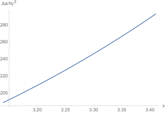
  Figure 1: The difference of the $a$ central charges between the supposedly UV fixed point $D_{6}$ and the supposedly IR fixed point $M_{2}$.

• it is the second term of (4.1) which dominates over the first one:

  $$W=Tr\,\left(XY^{2}+X^{k}Y\right)$$ (4.4)

  This case gives the $R$-charges of the adjoints the same as in $D_{2k}$. By assuming that (4.4) has also a dual in the present classification through the cyclotomic polynomials, than this is the theory $D_{2k}$.

In short, the new candidate for a fixed point $M_{k}$ can be a low energy limit of $D_{2k+2}$ with a perturbation (4.2) added, presumably for a large enough ratio of the Yukawas $y_{X^{2k+1}}/y_{XY^{2}}$.

4.2 The chiral ring

It is strange that all the mesons we need for the duality of the case in section 3.4.3 are just $\alpha=k$, i.e. $\tilde{Q}X^{j-1}Q$ for $j=1,\ldots,k$. In fact, the superpotential is

$$W=Tr\left(X^{2k+1}+X^{k}Y\right)$$ (4.5)

The e.o.m. for this system are

$$\frac{\partial W}{\partial X} = X^{2k}+X^{k-1}Y+X^{k-2}YX+\ldots+XYX^{k-2}+YX^{k-1}\propto I$$ (4.6)

$$\frac{\partial W}{\partial Y} = X^{k}\propto I$$ (4.7)

from which it is not clear among others why there is no $Y$ in the mesons.

As an example we will now consider the case $k=2$. Following [31, 7] we can easily see that classically at most single powers of $X$ and $Y$ are independent, while (4.6) for $k=2$ tells us that $X$ and $Y$ anticommute (modulo identity operator). So the possible mesons are naively

$$\tilde{Q}X^{i-1}Y^{m-1}Q\;\;\;,\;\;\;i=1,2\;\;\;,\;\;\;m=1,2$$ (4.8)

But this is only apparent, which we will see now, following the suggestion of [10], through the superconformal index. To keep track of the gauge invariant terms we use an expansion of (2.15) with the following values for the electric theory

$$f_{E}(w^{n}) =\frac{(Ft^{2})^{n}+(d_{+}\lambda_{-}t^{2})^{n}-(t\lambda_{+})^{n}-(t\lambda_{-})^{n}+\sum_{a=1}^{N_{A}}\left((X_{a}t^{R_{a}})^{n}-(\bar{\psi}_{X_{a}}t^{2-R_{a}})^{n}\right)}{\left(1-(td_{+})^{n}\right)\left(1-(td_{-})^{n}\right)}$$ (4.9)

$$g_{E}(w^{n}) =\frac{(Qt^{R_{Q}})^{n}p_{N_{f}}(y^{n})-(\bar{\psi}_{\tilde{Q}}t^{2-R_{Q}})^{n}p_{N_{f}}(\tilde{y}^{n})}{\left(1-(td_{+})^{n}\right)\left(1-(td_{-})^{n}\right)}v^{n}$$ (4.10)

$$\bar{g}_{E}(w^{n}) =\frac{(\tilde{Q}t^{R_{Q}})^{n}p_{N_{f}}(\tilde{y}^{-n})-(\bar{\psi}_{Q}t^{2-R_{Q}})^{n}p_{N_{f}}(y^{-n})}{\left(1-(td_{+})^{n}\right)\left(1-(td_{-})^{n}\right)}v^{-n}$$ (4.11)

where we denoted by $\bar{\psi}_{X,Y}$ the anti-fermions of the adjoints $X,Y$, by $d_{+,-}$ the derivatives, by $\lambda_{+,-}$ the gauginos (with only one combination among $d_{+}\lambda_{-}$ and $d_{-}\lambda_{+}$ independent due to the equation of motion [16, 14]) and $F$ the gauge field strength.

Eqs. (4.9), (4.10) and (4.11) have been derived from (2.6), (2.7) and (2.8) by explicitly denoting the origin of each single term (the fugacity $x$ ($x^{-1}$) has been replaced by $d_{+}$ ($d_{-}$) or $\lambda_{+}$ ($\lambda_{-}$)), following for example [16], see also table 2 of [14] and table 1 of [32] for a list of elements which contribute to the counting.

Now we can expand (2.15) as

$${\cal I}_{E}(w)={\cal I}_{E}^{(0)}(t)+{\cal I}_{E}^{(1)}(t)\left(\tilde{Q}Q\,t^{2R_{Q}}p_{N_{f}}(y)p_{N_{f}}(\tilde{y}^{-1})+\ldots\right)+\ldots$$ (4.12)

First we see the gauge invariant operators without the quark fields by expanding in powers of $t$:

$${\cal I}_{E}^{(0)} = 1+t^{4/5}X^{2}+t^{6/5}\left(X^{3}-X\bar{\psi}_{Y}\right)-\left(\lambda_{-}+\lambda_{+}\right)t^{7/5}X+t^{8/5}X\left(-X\bar{\psi}_{Y}+2X^{3}+Y\right)$$ (4.13)

$$+ t^{9/5}\left(\lambda_{-}\left(\bar{\psi}_{Y}-X^{2}\right)+\lambda_{+}\bar{\psi}_{Y}+d_{-}X^{2}+d_{+}X^{2}-\lambda_{+}X^{2}\right)$$

$$+ t^{2}\left(-2X^{3}\bar{\psi}_{Y}-X\bar{\psi}_{X}+X\bar{\psi}_{Y}^{2}-Y\bar{\psi}_{Y}+\lambda_{-}\lambda_{+}+2X^{5}+X^{2}Y\right)+O\left(t^{11/5}\right)$$

while the index of the terms proportional to $\tilde{Q}Q$ is

$${\cal I}_{E}^{(1)} = 1+t^{2/5}X+t^{4/5}\left(2X^{2}-\bar{\psi}_{Y}\right)+t\left(2d_{-}+2d_{+}-\lambda_{-}-\lambda_{+}\right)+t^{6/5}\left(-3X\bar{\psi}_{Y}+3X^{3}+Y\right)$$ (4.14)

$$+ 3t^{7/5}X\left(d_{-}+d_{+}-\lambda_{-}-\lambda_{+}\right)+t^{8/5}\left(-6X^{2}\bar{\psi}_{Y}-\bar{\psi}_{X}+\bar{\psi}_{Y}^{2}+5X^{4}+3XY\right)$$

$$+ t^{9/5}\left(d_{-}\left(7X^{2}-3\bar{\psi}_{Y}\right)-3d_{+}\bar{\psi}_{Y}+\lambda_{-}\left(3\bar{\psi}_{Y}-6X^{2}\right)+3\lambda_{+}\bar{\psi}_{Y}+7d_{+}X^{2}-6\lambda_{+}X^{2}\right)$$

$$+ t^{2}\left(-11X^{3}\bar{\psi}_{Y}-3X\bar{\psi}_{X}+5X\bar{\psi}_{Y}^{2}-3Y\bar{\psi}_{Y}+d_{-}\left(4d_{+}-3\lambda_{-}-3\lambda_{+}\right)-3d_{+}\lambda_{+}\right.$$

$$+ \left.\lambda_{-}\left(3\lambda_{+}-2d_{+}\right)+3d_{-}^{2}+3d_{+}^{2}+F+\lambda_{-}^{2}+\lambda_{+}^{2}+7X^{5}+6X^{2}Y\right)+O\left(t^{11/5}\right)$$

The first term in (4.14), i.e. $1$, means the operator $\tilde{Q}Q$. The second term, $X$, represents the operator $\tilde{Q}XQ$. The third one, $2X^{2}-\bar{\psi}_{Y}$, means that there is the operator $\tilde{Q}Q\,Tr(X^{2})$, while $\tilde{Q}X^{2}Q$ gets paired with $\tilde{Q}\bar{\psi}_{Y}Q$ forming a long multiplet and thus escaping the counting of the superconformal index, which is sensible only to short multiplets [13].

One can continue, finding that at each level only gauge invariant operators made out of $\tilde{Q}Q$ or $\tilde{Q}XQ$ multiplied by gauge invariant operators without quarks allowed by (4.13). For example, let’s see why there is no $\tilde{Q}YQ$ in the counting. This is a term of order $t^{6/5}$ in (4.14). The number of all gauge invariant operators coming from short multiplets of this order is $1$, distributed as

$$-3 : \tilde{Q}X\bar{\psi}_{Y}Q\;,\;\tilde{Q}\bar{\psi}_{Y}XQ\;,\;\tilde{Q}Q\,Tr(X\bar{\psi}_{Y})$$ (4.15)

$$+3 : \tilde{Q}X^{3}Q\;,\;\tilde{Q}XQ\,Tr(X^{2})\;,\;\tilde{Q}Q\,Tr(X^{3})$$ (4.16)

$$+1 : \tilde{Q}YQ$$ (4.17)

We know from the term of order $t^{6/5}$ of (4.13) that the last term of (4.15) pairs with the last term of (4.16). Thus the only multi trace term remained and allowed by (4.13) is $\tilde{Q}XQ\,Tr(X^{2})$, so there is no room for $\tilde{Q}YQ$ to survive unpaired.

The reader can continue in this fashion: the absence of $\tilde{Q}XYQ$ as a short multiplet is simply because the only 2 possibilities are

$$\tilde{Q}Q\,\left(Tr(X^{2})\right)^{2}\;,\;\tilde{Q}Q\,Tr(XY)$$ (4.18)

which are products of already allowed terms.

In other words, the only single trace operators made out of one quark $Q$ and one antiquark $\tilde{Q}$ are exactly $\tilde{Q}Q$ and $\tilde{Q}XQ$, and no others, in accord with the meson operators with $R$-charge $2R_{Q}+R_{j}$ needed in the magnetic theory. So the naive expectation from the classical equations of motion for the mesons present is misleading. Quantum constraints take care of this, which can be explicitly seen in the expansion of the superconformal index, as suggested in [10] and presented here for the case of interest.

5 Conclusions

Which are the possible fixed points in SQCD theories with $N_{A}$ ($\geq 0$) adjoints? A list of them, all connected to a UV free theory, can be found in [1, 8, 7]. All of them except the cases denoted by $E_{6}$ and $E_{8}$ [10] have a known candidate for a dual theory. In this work we gave a complete parametrisation of all such theories with a prescribed dual, assuming the adjoints’ $R$-charges are rational numbers in the interval between $0$ and $2$. These solutions include all known cases and give new ones. A family of new such solutions have been given, as well as possible suggestions on where these new solutions could lay on the tree of flows.

It is not clear from the classification whether there exist different classes of solutions to those presented in this work. The reason is that at least in principle one should go through an ordered but infinite number of possibilities, and check whether they are new or already in the known families. The mathematical problem boils down to possible classification of all products of distinct cyclotomic polynomials with positive coefficients. We do not know a solution.

In this work we limited the adjoints’ charges to rational numbers in the interval between $0$ and $2$. The choice of the rational numbers is mandatory for the classification of the solutions through the factorisation of the polynomial $y^{n}-1$ into products of cyclotomic polynomials, while the choice of the interval $[0,2]$ is less obvious. The motivation for it has two reasons.

First, in many cases it might be difficult to find a superpotential that enforces negative $R$-charges. For example, the solution of section 3.3.1 can be formally enlarged to $k<-1$. However we do not know of a superpotential with positive powers of the fields which would enforce it, unless one uses extra singlets.

A second, and, in our opinion, more important reason is that it is difficult to define a sensible superconformal index. Due to negative powers of the fugacity $t$ the superconformal index does not have a Taylor expansion in powers of $t$ around the origin. This, among others, means that even the derivation of eq. (2.17) is not guaranteed. We plan to look at this problem better in future, although it may well be that such $R$-charges outside the domain $[0,2]$ are simply forbidden.

In this work we limited ourselves to theories with at most two adjoints ($N_{A}\leq 2$). Of course it is straighforward to find solutions for general $N_{A}$, and we did it. The problem is that these theories are not asymptotically free and so, if connected to the free theory, typically violate the $a$-theorem. The only exceptions found so far are theories with at least some adjoints’ $R$-charges negative. These could represent examples of UV dual fixed points, i.e. examples of UV safety [34] in supersymmetric theories [35, 36, 37, 38]. Due to the difficult interpretation of these cases we leave also this analysis for the future.

Last but not least, all the analysis of this paper is done in the leading large $N_{c}$ limit. Only in this case the equality of the electric and magnetic superconformal indices reduces to a simple and easily calculable expression. So even the original equation (2.17) or equivalently (3.1), from which we started the analysis, is not known in general for finite $N_{c}$ and to get it requires much more effort, which is beyond the scope of this paper. On one side it is in principle possible that the new solutions $M_{k}$ (and/or $N_{k}$) are just an artifact of the large $N_{c}$ expansion and disappear when finite number of colours are considered. On the other side we are optimistic since the known solutions $D_{k+2}$ and $E_{7}$ persist for finite $N_{c}$, although clearly there is no guarantee that this is true also for the new candidate $M_{k}$.

Acknowledgments

We acknowledge the financial support from the Slovenian Research Agency (research core funding No. P1-0035). We thank Steve Abel and Francesco Sannino for discussion on various issues considered in this paper.

Appendix A A list of cyclotomic polynomials

For convenience we explicitly present here all the cyclotomic polynomials up to $n=30$. This choice of the upper $n$ is not dictated by what one can find in [17], but by the value needed for $E_{7}$ in section 3.4.2.

$$\Phi_{1}(y) =y-1$$

$$\Phi_{2}(y) =y+1$$

$$\Phi_{3}(y) =y^{2}+y+1$$

$$\Phi_{4}(y) =y^{2}+1$$

$$\Phi_{5}(y) =y^{4}+y^{3}+y^{2}+y+1$$

$$\Phi_{6}(y) =y^{2}-y+1$$

$$\Phi_{7}(y) =y^{6}+y^{5}+y^{4}+y^{3}+y^{2}+y+1$$

$$\Phi_{8}(y) =y^{4}+1$$

$$\Phi_{9}(y) =y^{6}+y^{3}+1$$

$$\Phi_{10}(y) =y^{4}-y^{3}+y^{2}-y+1$$

$$\Phi_{11}(y) =y^{10}+y^{9}+y^{8}+y^{7}+y^{6}+y^{5}+y^{4}+y^{3}+y^{2}+y+1$$

$$\Phi_{12}(y) =y^{4}-y^{2}+1$$

$$\Phi_{13}(y) =y^{12}+y^{11}+y^{10}+y^{9}+y^{8}+y^{7}+y^{6}+y^{5}+y^{4}+y^{3}+y^{2}+y+1$$

$$\Phi_{14}(y) =y^{6}-y^{5}+y^{4}-y^{3}+y^{2}-y+1$$

$$\Phi_{15}(y) =y^{8}-y^{7}+y^{5}-y^{4}+y^{3}-y+1$$

$$\Phi_{16}(y) =y^{8}+1$$

$$\Phi_{17}(y) =\sum_{i=1}^{17}y^{i-1}$$

$$\Phi_{18}(y) =y^{6}-y^{3}+1$$

$$\Phi_{19}(y) =\sum_{i=1}^{19}y^{i-1}$$

$$\Phi_{20}(y) =y^{8}-y^{6}+y^{4}-y^{2}+1$$

$$\Phi_{21}(y) =y^{12}-y^{11}+y^{9}-y^{8}+y^{6}-y^{4}+y^{3}-y+1$$

$$\Phi_{22}(y) =y^{10}-y^{9}+y^{8}-y^{7}+y^{6}-y^{5}+y^{4}-y^{3}+y^{2}-y+1$$

$$\Phi_{23}(y) =\sum_{i=1}^{23}y^{i-1}$$

$$\Phi_{24}(y) =y^{8}-y^{4}+1$$

$$\Phi_{25}(y) =y^{20}+y^{15}+y^{10}+y^{5}+1$$

$$\Phi_{26}(y) =y^{12}-y^{11}+y^{10}-y^{9}+y^{8}-y^{7}+y^{6}-y^{5}+y^{4}-y^{3}+y^{2}-y+1$$

$$\Phi_{27}(y) =y^{18}+y^{9}+1$$

$$\Phi_{28}(y) =y^{12}-y^{10}+y^{8}-y^{6}+y^{4}-y^{2}+1$$

$$\Phi_{29}(y) =\sum_{i=1}^{29}y^{i-1}$$

$$\Phi_{30}(y) =y^{8}+y^{7}-y^{5}-y^{4}-y^{3}+y+1$$ (A.1)

Appendix B A proof that $\alpha>0$ and a sum rule

One could worry that the quantity $\alpha$ defined in (3.24) may not be positive, and thus invalidate the consistency. Here we show that it is always positive, as it must be. It follows from the general property of the cyclotomic polynomials for $n>1$ ($\Phi_{1}(1)=0$):

$$\Phi_{n}(1) = 1\;\;{\rm if}\;n\;{\rm is\;not\;a\;prime\;power}$$ (B.1)

$$\Phi_{n}(1) = p\;\;{\rm if}\;n=p^{k}\;{\rm is\;a\;prime\;power\;with}\;k\geq 1$$

This means that any product of cyclotomic polynomials with $n\neq 1$ is positive at $y=1$. In our case

$$\left.\frac{\Phi_{n}^{-}(y)}{y-1}\right|_{y\to 1}>0$$ (B.2)

But we can expand

$$\frac{\Phi_{n}^{-}(y)}{y-1} = \frac{1}{y-1}\sum_{a=1}^{N_{A}+1}\left(y^{p_{a}}-y^{m-p_{a}}\right)$$ (B.3)

$$= \frac{1}{y-1}\sum_{a=1}^{N_{A}+1}\left(\Theta(2p_{a}-m)y^{m-p_{a}}\left(y^{2p_{a}-m}-1\right)-\Theta(m-2p_{a})y^{p_{a}}\left(y^{m-2p_{a}}-1\right)\right)$$

$$= \sum_{a=1}^{N_{A}+1}\left(\Theta(2p_{a}-m)\sum_{j=0}^{2p_{a}-m-1}y^{m-p_{a}+j}-\Theta(m-2p_{a})\sum_{j=0}^{m-2p_{a}-1}y^{p_{a}+j}\right)$$

Taking it at $y=1$ we get

$$\left.\frac{\Phi_{n}^{-}(y)}{y-1}\right|_{y\to 1} = \sum_{a=1}^{N_{A}+1}\left(\Theta(2p_{a}-m)(2p_{a}-m)-\Theta(m-2p_{a})(m-2p_{a})\right)$$ (B.4)

$$= \sum_{a=1}^{N_{A}+1}\left(2p_{a}-m\right)$$

which in combination with (B.2) gives

$$\sum_{a=1}^{N_{A}+1}\left(2p_{a}-m\right)>0$$ (B.5)

Eq. (3.24) (remember that $m=p_{N_{A}+1}$) finally proves that $\alpha>0$.

From here it immediately follows a sum rule for $\sum_{a=1}^{N_{A}+1}\left(R_{a}-1\right)$. Since

$$\sum_{a=1}^{N_{A}+1}\left(R_{a}-1\right)=\frac{1}{p_{N_{A}+1}}\sum_{a=1}^{N_{A}+1}\left(2p_{a}-p_{N_{A}+1}\right)$$ (B.6)

due to (B.5) we also find that

$$\sum_{a=1}^{N_{A}+1}\left(R_{a}-1\right)>0$$ (B.7)

This gives a necessary (although not suffficient) criterium which any given set of adjoints’ $R$-charges, which represent a Seiberg-Kutasov dual theory, must satisfy. For example the choice $R_{a}=(1/6,1/3)$ cannot. In fact for this case $\sum_{a=1}^{3}=(1/6-1)+(1/3-1)+(2-1)=-1/2<0$ and thus violates the sum rule B.7.

Appendix C Redundancy

Let $n$ be the product of two prime numbers $p_{1,2}$ and an integer $r>0$:

$$n=rp_{1}p_{2}$$ (C.1)

Then choose

$$\Phi_{n}^{-}(y)=\Phi_{1}(y^{r})\Phi_{p_{1}p_{2}}(y^{r})$$ (C.2)

The divisors of $p_{1}p_{2}$ are $1$, $p_{1}$, $p_{2}$ and $p_{1}p_{2}$, so

$$\Phi_{n}^{+}(y)=\frac{y^{n}-1}{\Phi^{-}(y)}=\Phi_{p_{1}}(y^{r})\Phi_{p_{2}}(y^{r})$$ (C.3)

has all coefficients positive, since for any prime $p$

$$\Phi_{p}(x)=\sum_{i=1}^{p}x^{(i-1)}$$ (C.4)

With

$$y^{r(1+\varphi(p_{1}p_{2}))}=t^{2}$$ (C.5)

equation (2.17) now becomes

$$\Phi_{1}\left(t^{\frac{2}{1+\varphi(p_{1}p_{2})}}\right)\Phi_{p_{1}p_{2}}\left(t^{\frac{2}{1+\varphi(p_{1}p_{2})}}\right)=\frac{t^{\frac{2p_{1}p_{2}}{1+\varphi(p_{1}p_{2})}}-1}{\Phi_{p_{1}}\left(t^{\frac{2}{1+\varphi(p_{1}p_{2})}}\right)\Phi_{p_{2}}\left(t^{\frac{2}{1+\varphi(p_{1}p_{2})}}\right)}$$ (C.6)

with $\varphi(n)$ the $n^{th}$ Euler’s totient function. Once $p_{1,2}$ are fixed, solution (C.2) does not lead to new solutions for different $r$. Of course, the ansatz (C.2) is only one possibility, and others are possible, among them for example ${\cal D}_{n}^{-}=\{1,p_{1},p_{1}p_{2}\}$ or ${\cal D}_{n}^{-}=\{1,p_{2},p_{1}p_{2}\}$.

The main message is that increasing $n$ does not necessarily give new solutions. This might mean that the number of families is finite and thus in some future possible to determine all of them.

References

• [1] N. Seiberg, “Electric–magnetic Duality in Supersymmetric Nonabelian Gauge Theories,” Nucl. Phys. B 435 (1995) 129 [hep-th/9411149].
• [2] D. Kutasov, “A Comment on Duality in ${\mathcal{N}}\!=1$ Supersymmetric Nonabelian Gauge Theories,” Phys. Lett. B 351 (1995) 230 [hep-th/9503086].
• [3] D. Kutasov and A. Schwimmer, “On Duality in Supersymmetric Yang-Mills Theory,” Phys. Lett. B 354 (1995) 315 [hep-th/9505004].
• [4] D. Kutasov, A. Schwimmer and N. Seiberg, “Chiral Rings, Singularity Theory and Electric–magnetic Duality,” Nucl. Phys. B 459 (1996) 455 [hep-th/9510222].
• [5] J. H. Brodie, “Duality in Supersymmetric $SU(\hbox{$N_{c}$}$) Gauge Theory with Two Adjoint Chiral Superfields,” Nucl. Phys. B 478 (1996) 123 [hep-th/9605232].
• [6] J. H. Brodie and M. J. Strassler, “Patterns of Duality in ${\mathcal{N}}\!=1$ SUSY Gauge Theories, Or: Seating Preferences of Theater Going Nonabelian Dualities,” Nucl. Phys. B 524 (1998) 224 [hep-th/9611197].
• [7] K. A. Intriligator and B. Wecht, “RG Fixed Points and Flows in Sqcd with Adjoints,” Nucl. Phys. B 677 (2004) 223 [hep-th/0309201].
• [8] D. Kutasov, A. Parnachev and D. A. Sahakyan, “Central Charges and U(1)(R) Symmetries in ${\mathcal{N}}\!=1$ Superyang-Mills,” JHEP 0311 (2003) 013 [hep-th/0308071].
• [9] D. Kutasov and J. Lin, “Exceptional ${\mathcal{N}}\!=1$ Duality,” arXiv:1401.4168 [hep-th].
• [10] D. Kutasov and J. Lin, “${\mathcal{N}}\!=1$ Duality and the Superconformal Index,” arXiv:1402.5411 [hep-th].
• [11] L. Mazzucato, “Chiral Rings, Anomalies and Electric-Magnetic Duality,” JHEP 0411 (2004) 020 [hep-th/0408240].
• [12] L. Mazzucato, “Remarks on the Analytic Structure of Supersymmetric Effective Actions,” JHEP 0512 (2005) 026 [hep-th/0508234].
• [13] C. Romelsberger, “Counting Chiral Primaries in ${\mathcal{N}}\!=1$, $d=4$ Superconformal Field Theories,” Nucl. Phys. B 747 (2006) 329 [hep-th/0510060].
• [14] J. Kinney, J. M. Maldacena, S. Minwalla and S. Raju, “An Index for 4 Dimensional Super Conformal Theories,” Commun. Math. Phys.  275 (2007) 209 [hep-th/0510251].
• [15] C. Romelsberger, “Calculating the Superconformal Index and Seiberg Duality,” arXiv:0707.3702 [hep-th].
• [16] F. A. Dolan and H. Osborn, “Applications of the Superconformal Index for Protected Operators and Q-Hypergeometric Identities to ${\mathcal{N}}\!=1$ Dual Theories,” Nucl. Phys. B 818 (2009) 137 [arXiv:0801.4947 [hep-th]].
• [17] For a fast introduction see for example https://en.wikipedia.org/wiki/Cyclotomic_polynomial and references therein.
• [18] L. Rastelli and S. S. Razamat, “The Supersymmetric Index in Four Dimensions,” J. Phys. A 50 (2017) no.44, 443013 [arXiv:1608.02965 [hep-th]].
• [19] V. P. Spiridonov and G. S. Vartanov, “Elliptic Hypergeometry of Supersymmetric Dualities,” Commun. Math. Phys. 304 (2011) 797 [arXiv:0910.5944 [hep-th]].
• [20] K. A. Intriligator and B. Wecht, “The Exact Superconformal R Symmetry maximizes $a$,” Nucl. Phys. B 667 (2003) 183 [hep-th/0304128].
• [21] D. Anselmi, J. Erlich, D. Z. Freedman and A. A. Johansen, “Positivity Constraints on Anomalies in Supersymmetric Gauge Theories,” Phys. Rev. D 57 (1998) 7570 [hep-th/9711035].
• [22] D. M. Hofman and J. Maldacena, “Conformal Collider Physics: Energy and Charge Correlations,” JHEP 0805 (2008) 012 [arXiv:0803.1467 [hep-th]].
• [23] A. B. Zamolodchikov, “Irreversibility of the Flux of the Renormalization Group in a 2D Field Theory,” JETP Lett.  43 (1986) 730 [Pisma Zh. Eksp. Teor. Fiz.  43 (1986) 565].
• [24] J. L. Cardy, “Is There a $c$-Theorem in Four-Dimensions?,” Phys. Lett. B 215 (1988) 749.
• [25] H. Osborn, “Derivation of a Four-Dimensional $c$ Theorem,” Phys. Lett. B 222 (1989) 97.
• [26] I. Jack and H. Osborn, “Analogs for the $c$ Theorem for Four-Dimensional Renormalizable Field Theories,” Nucl. Phys. B 343 (1990) 647.
• [27] Z. Komargodski and A. Schwimmer, “On Renormalization Group Flows in Four Dimensions,” JHEP 1112 (2011) 099 [arXiv:1107.3987 [hep-th]].
• [28] Z. Komargodski, “The Constraints of Conformal Symmetry on RG Flows,” JHEP 1207 (2012) 069 [arXiv:1112.4538 [hep-th]].
• [29] R. G. Leigh and M. J. Strassler, “Exactly Marginal Operators and Duality in Four-Dimensional ${\mathcal{N}}\!=1$ Supersymmetric Gauge Theory,” Nucl. Phys. B 447 (1995) 95 [hep-th/9503121].
• [30] M. J. Strassler, “The Duality Cascade,” hep-th/0505153.
• [31] F. Cachazo, S. Katz and C. Vafa, “Geometric Transitions and ${\mathcal{N}}\!=1$ Quiver Theories,” hep-th/0108120.
• [32] A. Gadde, L. Rastelli, S. S. Razamat and W. Yan, “On the Superconformal Index of ${\mathcal{N}}\!=1$ IR Fixed Points: a Holographic Check,” JHEP 1103 (2011) 041 [arXiv:1011.5278 [hep-th]].
• [33] G. Mack, “All Unitary Ray Representations of the Conformal Group $SU(2,2)$ with Positive Energy,” Commun. Math. Phys.  55 (1977) 1.
• [34] D. F. Litim and F. Sannino, “Asymptotic Safety Guaranteed,” JHEP 1412 (2014) 178 [arXiv:1406.2337 [hep-th]].
• [35] K. Intriligator and F. Sannino, “Supersymmetric Asymptotic Safety is Not Guaranteed,” JHEP 1511 (2015) 023 [arXiv:1508.07411 [hep-th]].
• [36] B. Bajc and F. Sannino, “Asymptotically Safe Grand Unification,” JHEP 1612 (2016) 141 [arXiv:1610.09681 [hep-th]].
• [37] A. D. Bond and D. F. Litim, “Asymptotic Safety Guaranteed in Supersymmetry,” Phys. Rev. Lett.  119 (2017) no.21, 211601 [arXiv:1709.06953 [hep-th]].
• [38] B. Bajc, N. A. Dondi and F. Sannino, “Safe Susy,” JHEP 1803 (2018) 005 [arXiv:1709.07436 [hep-th]].