Statistical mechanics of asymmetric tethered membranes: spiral and crumpled phases

Abstract

We develop the elastic theory for inversion-asymmetric tethered membranes and use it to identify and study their possible phases. Asymmetry in a tethered membrane causes spontaneous curvature, which in general depends upon the local in-plane dilation of the tethered network. This in turn leads to long-ranged interactions between the local mean and Gaussian curvatures, which is not present in symmetric tethered membranes. This interplay between asymmetry and Gaussian curvature leads to a new double-spiral phase not found in symmetric tethered membranes. At temperature $T=0$, tethered membranes of arbitrarily large size are always rolled up tightly into a conjoined pair of Archimedes’ spirals. At finite $T$ this spiral structure swells up significantly into algebraic spirals characterized by universal exponents which we calculate. These spirals have long range orientational order, and are the asymmetric analogs of statistically flat symmetric tethered membranes. We also find that sufficiently strong asymmetry can trigger a structural instability leading to crumpling of these membranes as well. This provides a new route to crumpling for asymmetric tethered membranes. We calculate the maximum linear extent $L_{c}$ beyond which the membrane crumples, and calculate the universal dependence of $L_{c}$ on the membrane parameters. By tuning the asymmetry parameter, $L_{c}$ can be continuously varied, implying a scale-dependent crumpling. Our theory can be tested on controlled experiments on lipids with artificial deposits of spectrin filaments, in-vitro experiments on red blood cell membrane extracts, and on graphene coated on one side.

I Introduction

The statistical mechanics of membranes has long generated considerable theoretical and experimental interest Nelson et al. (2004). In contrast to linear polymers Cates (1984, 1985), fluctuating surfaces can exhibit a wide variety of different phases, depending on rigidity, surface tension, and various microscopic constraints. Polymerized or tethered membranes, are particularly interesting Nelson et al. (2004); Kantor et al. (1987). These are two-dimensional (2D) analogs of linear polymer chains. But, unlike polymers, which are always coiled up, tethered membranes at low temperatures ($T$) or high bending rigidity are known Nelson et al. (2004); Paczuski et al. (1988) to display a statistically flat phase with long range orientational order in the surface normals. Notice that the very existence of a 2D flat phase is surprising, since the well-known Hohenberg-Mermin-Wagner (HMW) theorem forbids spontaneous symmetry breaking for two dimensional systems with a continuous symmetry Mermin and Wagner (1966); Hohenberg (1967). This apparent violation of the HMW theorem is possible due to the coupling between the in-plane elastic degrees of freedom and the out-of-plane undulations, which introduces an effective long-ranged interaction between the undulation modes. Since the HMW theorem only applies for systems with short-ranged interactions, this long-ranged interaction allows tethered membranes to have the long-ranged orientational order that must occur in a flat phase. At higher temperature, tethered membranes possibly show a phase transition to a crumpled phase Nelson et al. (2004); Guitter et al. (1989); David and Wiese (1996); Wiese and David (1997), although the existence of the latter remains controversial even now Domb (2000).

Most theoretical studies of tethered membranes to date that we know of have considered only inversion-symmetric membranes, i.e., membranes that are identical on both sides. Many real membranes, e.g., graphene coated on one side by some substance (e.g., polymer or a layer of lipid) and both in-vivo red blood cell membranes and in-vitro spectrin-deposited model lipid bilayers López-Montero et al. (2012) are structurally inversion asymmetric. The effects of such asymmetry are still largely unexplored theoretically.

In this paper, we develop a generic and experimentally testable theory of equilibrium asymmetric tethered membranes. We find that such membranes exhibit a new ”spiral state” not found in symmetric membranes. As illustrated in Fig. 1, the mean spatial configuration of this state can be obtained by joining two coplanar spirals of opposite handedness at their base, and extruding that curve in the direction perpendicular to the plane of the spirals.

The shape of the spirals in the spiral state is universal. First consider membranes for which thermal fluctuations are negligible (i.e., membranes that are effectively at temperature $T=0$). Such asymmetric membranes of large linear size $L_{m}$ spontaneously arrange themselves into a double spiral of ArchimedesArchimedes (-225) structure: 

$$r(\theta)=r_{0}+a{\theta\over 2\pi},$$ (I.1)

where $r(\theta)$ is the radius of the spiral from its center to a point on the spiral at which the radius is being determined and $\theta$ is the angle of that point in the anticlockwise direction as shown in Fig. 1 (left) for the right-hand spiral, and in the clockwise direction for the left hand spiral, with $\theta=0$ being the innermost edge of the membrane; see Fig. 1 (right) for a schematic picture of a double spiral.

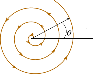
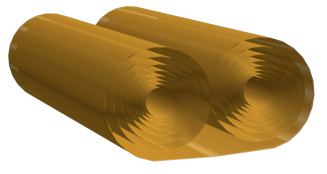
Figure 1: (Color online)(top) Schematic diagram of the cross section of a spiral, (bottom) Schematic diagram of the double spiral structure of our model membrane.

In (I.1), $a$ is the thickness of the membrane. Choosing this form for $r(\theta)$ simply means that the membrane is curled up as tightly as it can, given excluded volume effects. In (I.1), the size $r_{0}$ of the hole left in the center of the spiral is given by

$$r_{0}={\kappa_{0}\over 2C}.$$ (I.2)

where $\kappa_{0}$ is the ”bare” bend modulus of the membrane (to be defined formally below) and $C$ is a phenomenological ”spontaneous curvature” parameter which is a measure of the asymmetry of the membrane, and will also be defined more precisely below. Since $r_{0}$ is independent of the size of the membrane, it is always negligible compared to the outer radius of the spiral for a sufficiently large membranes ($L_{m}\gg r_{0}$). Thus, one can effectively consider the spiral to extend all the way into the origin.

Thermal fluctuations considerably change this picture. For membranes with sufficiently small asymmetry, thermal fluctuations open up the spiral by giving rise to a longer ranged ”Helfrich repulsion”Helfrich (1978); the resultant form of the the spiral is:

$$r(\theta)=R_{0}\theta^{\nu},$$ (I.3)

where the universal exponent $\nu$ is related to the equally universal exponent $\eta$ characterizing the anomalous bend elasticity Nelson et al. (2004) of symmetric membranes through the relation

$$\nu={4\over 2+\eta}{\approx 4-{2\over 3}\sqrt{15}\approx 1.418}\,,$$ (I.4)

where the numerical estimate is based on the theoretical estimate

$$\eta\approx{4\over 1+\sqrt{15}}\approx.821$$ (I.5)

obtained by Le Doussal and Radzihovsky Doussal and Radzihovsky (1992). For a large enough spiral, consecutive segments of size smaller than $\kappa/C$ appear nearly flat, and hence behave like a stack of symmetric membranes locally. In addition, the scale length $R_{0}$ exhibits universal scaling with temperature and other parameters, which can also be related exactly to the exponent $\eta$; we find

$$R_{0} = \left[(k_{B}T)^{2(2-\eta)}\kappa_{0}^{2(\eta-1)}A_{0}^{-{\eta}}C^{(\eta-2)}\right]^{1/(2+\eta)}\times{\cal O}(1)\,,$$ (I.6)

$$= (k_{B}T)^{.836}\kappa_{0}^{-.127}A_{0}^{-.291}C^{-.418}\times{\cal O}(1)\,,$$

where $\kappa_{0}$ is the ”bare” bend modulus (to be defined formally below) and $A_{0}\equiv\frac{4\mu_{0}(\mu_{0}+\lambda_{0})}{2\mu_{0}+\lambda_{0}}>0$, with $\mu_{0}$ and $\lambda_{0}$ the equally bare two-dimensional Lame’ elastic coefficients of the membrane. Here, by “bare”, we mean the values these parameters have before being renormalized by thermal fluctuation effects. The numerical values for the exponents quoted in the second line are based on the estimate (I.5) of $\eta$.

All of the parameters in this paper, and the equations defining them, are summarized in the glossary that constitutes appendix (Appendix I: Glossary) of this paper.

The total radius $R_{T}$ of the spiral regions also exhibits universal scaling, in this case with the spatial extent $L_{m}$ of the membrane:

$$R_{T}=R_{0}^{1-\alpha}L_{m}^{\alpha}\,\,\,\,,\,\,\,\,\alpha\equiv{4\over 6+\eta}\approx 0.586\,\,.$$ (I.7)

The entire picture of the spiral state just described presupposes that each of the two spirals makes many turns. It therefore behooves us to ask how many turns $n$ the spirals formed by a membrane of length $L_{m}$ actually make. Assuming this number is large, it is easily found by plugging the total radius $R$ obtained from (I.7) into our expression (I.3) for the spiral structure, equating $\theta$ on the right hand side of that expression to $2\pi n$, and solving for $n$. We thereby obtain

$$n(L_{m})={1\over 2\pi}\left({L_{m}\over R_{0}}\right)^{\alpha/\nu}={1\over 2\pi}\left({L_{m}\over R_{0}}\right)^{\varpi}\,,$$ (I.8)

where we have defined another universal exponent

$$\varpi\equiv{\alpha\over\nu}={2+\eta\over 6+\eta}\approx 0.414\,.$$ (I.9)

Note that, based on our earlier expression for the length scale $R_{0}$, and the numerical estimate (I.5) of $\eta$, the number of turns is quite insensitive to material parameters

$$n(L_{m})\propto R_{0}^{-\varpi}\propto T^{-0.346}\kappa_{0}^{0.053}A_{0}^{0.12}C^{0.173}\,,$$ (I.10)

so we can estimate the number of turns fairly accurately even if there is a large uncertainty in the values of the material parameters. For example, consider a graphene sheet made asymmetrical by being coated with cholesterol. The Young’s modulus of graphene is Lee et al. (2008) $G=10^{12}$ Pa. If we model graphene as a bulk elastic sheet with this Young’s modulus and thickness Jussila et al. (2016) $a=3.7\AA$ (the interatomic distance), then we can estimate $\kappa_{0}\sim Ga^{3}=5\times 10^{-10}$ergs and $A_{0}\sim Ga=3.7{\times 10^{5}{{\rm dynes}\over{\rm cm}}}$. The parameter $C$ is trickier to estimate; if we assume that it is comparable to its value for pure cholesterol, and estimate that value by using the value of ${\kappa\over C}=2.9\times 10^{-9}{\rm m}$ for pure cholesterol (see table 2), and estimating $\kappa_{0}$ for pure c holesterol by the value of $\kappa_{0}=4\times 10^{-12}{\rm ergs}$ for DMPC (see table 2), we get $C=1.38\times 10^{-10}{\rm N}$. Using these values in blah for $R_{0}$ gives $R_{0}=2.54\times 10^{-12}{\rm m}$; using that in (I.8) gives $n=27\times\left({L_{m}\over 1\mu}\right)^{\varpi}=27\times\left({L_{m}\over 1\mu}\right)^{0.414}$.

One could very well question all of the above estimates of the material parameters $C$, $\kappa_{0}$, and $A_{0}$; but, due to the insensitivity of $n$ to those parameters, the estimate will not change very much: any membrane larger than about one micron should exhibit a sufficient number of turns for our theory to be valid.

This spiral state is not the only possible phase of an asymmetric membrane: we also find that asymmetric tethered membranes exhibit a crumpled phase. Indeed, we have discovered a novel structural instability in asymmetric membranes, in which asymmetry actually induces crumpling of the membrane Peliti and Leibler (1985); Nelson et al. (2004) More specifically, we find that sufficiently asymmetric tethered membranes in equilibrium become structurally unstable , yielding a crumpled state for sufficiently large asymmetry.

This instability is driven by the dependence of the local spontaneous curvature on the local dilation of the tethered network, a dependence that on symmetry grounds can only occur in asymmetric membranes. The strength of this dependence is given by a dilation-bend elastic coupling constant $\chi$ that can be used as a measure of the degree of asymmetry, since it is only non-zero in asymmetric membranes. The critical value of $\chi$ at which this effect of asymmetry drives crumpling is determined by the ”decoupled” bend modulus $\kappa^{\prime}$ where by “decoupled”, we mean the bend modulus the membrane would have in the absence of the dilation-bend elastic coupling constant $\chi$. The parameters $\kappa^{\prime}$ and $\chi$ are defined precisely in equation (II.1) below.

The phase diagram for an asymmetric membrane in the $\chi$-$\kappa^{\prime}$ plane is illustrated in Fig. 2a. To connect this diagram to experiments, we note that in general both $\kappa^{\prime}$ and $\chi$ should be functions of almost every imaginable experimental control parameter; e.g., temperature and salt concentration in the fluid around the membrane. If this function is analytic, which we expect it to be in general, then the topology of the phase diagram plotted as a function of any two experimental control parameters (e.g., temperature and salt concentration) will have the same topology as Fig. 2.

Note that this phase diagram has two distinct phase boundaries. The lower of these, $\chi_{{}_{{}_{L}}}(\kappa^{\prime})$, separates two distinct regimes of parameter space within this crumpled phase. In one of these, (hereafter called the “strongly crumpled” (SC) regime), the membrane will be crumpled no matter how small it is, while in the second (hereafter called, ”weakly crumpled” (WC)), it is only crumpled if its lateral spatial extent $L_{m}$ exceeds a critical size $L_{c}$. Smaller membranes (i.e., $L_{m}<L_{c}$) exhibit a spiral structure similar to that found in the spiral phase, but different in its scaling properties. This behavior is summarized in Fig. 2b.

If $\kappa_{0}\gg k_{B}T$, most of the boundary $L_{c}(\chi)$ between the crumpled and the spiral phases in Fig. (2)b obeys

$$L_{c}(\chi)\propto(\chi_{{}_{U}}^{2}-\chi^{2})^{7/2}\,.$$ (I.11)

This laws breaks down near the two limits $\chi\to\chi_{{}_{{}_{U}}}$, where $L_{c}$ gets to be $<R_{0}$, so no uncrumpled membrane can be long enough to wind up into a spiral, and as $\chi\to\chi_{{}_{{}_{L}}}$, where $L_{c}$ diverges. Unfortunately, this divergence is controlled by a perturbatively inaccessible fixed point, as illustrated in figure (9), so we can say nothing quantitative about the functional dependence of $L_{c}(\chi)$ as $\chi\to\chi_{{}_{{}_{L}}}$.

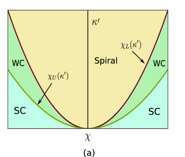
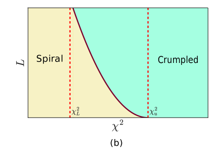
Figure 2: (Color online) a) Schematic phase diagram in the $\chi^{2}-\kappa^{\prime}$ plane.
b)The continuous curve (black) is the line $L=\xi(\chi^{2})$, demarcating the spiral and the crumpled phases.

We find that there are a hierarchy of length scales in asymmetric tethered membranes. While thermal fluctuations expand the spiral structure significantly from its $T=0$ shape, successive turns keep coming in contact with each other due to fluctuations. The smallest of the length scales in asymmetric tethered membranes is the “Helfrich length” $L_{H}$, which is the typical distance between “bumps” or points of contact; see Fig.3. For length scales $L\ll L_{H}$, the asymmetric membrane looks flat, and self avoiding interactions are therefore unimportantNelson et al. (2004).

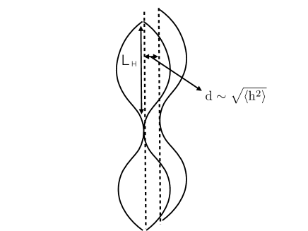
Figure 3: Schematic diagram depicting local patches of successive turns of spiral at finite $T$.The length scale $L_{H}$ is the typical distance between successive points of contact of neighboring layer, while $d\sim\sqrt{\langle h^{2}\rangle}$ is the typical distance between successive layers.

The remainder of this paper is organized as follows. In section (II), we formulate the elastic theory, and study the behavior, of asymmetric membranes for the smallest range of length scales described above (i.e., $L\ll L_{H}$). In section (III), we treat the largest length scales $L\gg L_{H}$, and determine the spiral structure, both for $T=0$, and $T\neq 0$. Section (III) also addresses crumpling, and demonstrates the existence of both the ”weakly crumpled” and ”strongly crumpled” regimes of parameter space, and the spiral structure of membranes in the ”weakly crumpled” regime that are small enough to avoid crumpling. In section (IV), we summarize our results and discuss possible future theoretical and experimental work.

II Small length scales $L\ll L_{H}$

In this section, we begin by formulating, in subsection (A), the elastic theory of asymmetric fluctuating membranes for length scales $L\ll L_{H}$, on which the membrane is nearly flat and non-self intersecting. This differs from that for symmetric membranes by the addition of the two up-down symmetry breaking terms mentioned in the introduction: the dilation-bend elastic coupling constant $\chi$, and the spontaneous curvature $C$. In subsection (B), we treat this model in the quadratic approximation, and demonstrate that sufficiently strong asymmetry can cause crumpling. In subsection (C), we go beyond the harmonic approximation, and use the Renormalization group (RG) to treat the effect of elastic anharmonicities. We show that these are relevant, in RG sense of changing the long distance behavior of the membrane, if the internal dimension $d$ of the membrane is less than four (as it is in the physical case $d=2$). We also find that for sufficiently small asymmetry, the membrane on length scales $L\ll L_{H}$ is controlled by the same RG fixed point as symmetric membranes; that is, the dilation-bend elastic coupling constant $\chi$ is irrelevant at long length scales, and the spontaneous curvature $C$, though relevant (i.e., growing upon renormalization), has not yet, at these short length scales, become important enough to matter. For larger asymmetry, the RG flows do not approach the symmetric membrane fixed point; we argue that this implies the membrane crumples at these asymmetries, even for some asymmetries small enough that the harmonic theory would suggest that the membrane remains uncrumpled.

II.1 Elastic free energy for $L\ll L_{H}$

We begin by formulating the elastic model for a single turn of the spiral structure, on length scales short compared to both the local radius of curvature $R$ and the typical distance $L_{H}$ between successive interactions of that turn with the turns inside and outside of it: a membrane segment of linear size $L\ll L_{H}$ behaves like an isolated, free membrane not in contact with anything else. The results of this analysis will then be used in section (III) as inputs to treat the membrane on progressively larger scales: first, to compute $L_{H}$, and thereby calculate the interaction between successive turns of the membrane, and then on length scales comparable to $R$, which will allow us to calculate the large scale spiral structure of the membrane.

On the smallest length scales $L$, we can ignore both self-avoidance interactions (since, by assumption, $L\ll L_{H}$) and the curvature of the membrane (since $L\ll R$). The latter simplification allows us to describe the membrane fluctuations in the so-called “Monge gauge”, which introduces a single-valued height field $h({\bf r})$ and an in-plane displacement by a 2D vector field ${\bf u}({\bf r})$, ${\bf r}=(x,y)$ with ${\bf R}(\mathbf{r})\equiv({\bf r}+\mathbf{u}({\bf r}),h(\bf r)$) denoting the new, post-fluctuation coordinates in the three-dimensional embedding space of a point on the membrane which was originally located at ${\bf R}(\mathbf{r})=(x,y,z=0)$ Nelson et al. (2004); Chaikin and Lubensky (2000).

General symmetry considerations then dictate the following form for the free energy functional ${\mathcal{F}}$ for tensionless asymmetric tethered membranes:

$${\mathcal{F}} = \frac{1}{2}\int d^{2}r\left[\kappa^{\prime}(\nabla^{2}h)^{2}+\lambda u_{ii}^{2}+2\mu u_{ij}u_{ij}+2\chi u_{ii}\nabla^{2}h\right]$$ (II.1)

$$+ \int d^{2}r\,\,C\nabla^{2}h$$

to leading order in gradients (see Appendix Appendix III: Rotationally invariant free energy for a fully rotationally invariant free energy functional that yields (II.1) in the nearly flat limit in the Monge gauge). Here $u_{ij}=\frac{1}{2}(\nabla_{i}u_{j}+\nabla_{j}u_{i}+\nabla_{i}h\nabla_{j}h)$ is the strain tensor, ignoring terms quadratic in $\nabla_{i}u_{j}$, which are irrelevant here in the renormalization group (RG) sense Chaikin and Lubensky (2000); Aronovitz and Lubensky (1988); Nelson et al. (2004).

The free energy (II.1), differs from that of symmetric membranes only by the addition of two generic inversion-symmetry breaking terms: a linear “spontaneous curvature” term $C\nabla^{2}h$, that makes the membrane want to curl up with a radius of curvature $R\propto 1/C$ and a term $\chi\nabla^{2}hu_{ii}$, that describes local bending of the membrane in response to local compression of the elastic network. Both these terms can be separately positive or negative, and arise naturally by expanding a local compression dependent curvature term $f(u_{ii})\nabla^{2}h$ to linear order in $u_{ii}$. A term analogous to our $\chi$ term was introduced for fluid membranes by Leibler (1986), a paper which inspired ours.

II.2 Quadratic theory and zero-temperature asymmetry induced crumpling

Up to quadratic order in the fields, the free energy (II.1) can be approximated as:

$${\mathcal{F}}\approx{\mathcal{F}}_{g} = \sum_{\mathbf{q}}[\frac{\kappa^{\prime}}{2}q^{4}|h({\bf q})|^{2}+(\frac{\lambda}{2}+\mu)q^{2}\{|u^{L}({\bf q})|^{2}$$ (II.2)

$$- \frac{2iq\chi h({\bf q})u^{L}({\bf-q})}{2\mu+\lambda}\}+\mu q^{2}|{\bf u}^{T}({\bf q})|^{2}],$$

where $h({\bf q})$, and ${\bf u}({\bf q})$ are the spatial Fourier transforms of $h({\bf r})$ and ${\bf u}({\bf r})$, with $u_{i}^{L}({\bf q})$ and $u_{i}^{T}({\bf q})$ the projections of ${\bf u}({\bf q})$ along and perpendicular to wavevector ${\bf q}$ respectively. Note that $C$ has dropped out of the problem at this point; this is because the spontaneous curvature term, in the Monge approximation, is just a total derivative, and hence becomes a surface term which does not affect the Fourier modes. Once we go to larger length scales $L\gg L_{H}$ at which the Monge approximation breaks down due to spontaneous curvature of the membrane, this term will come into play; indeed, it will control the shape of the membrane, as we will see in section (III) below.

Integrating the fields $u^{T}({\bf q})$ and $u^{L}({\bf q})$ out of the Gaussian (i.e., harmonic) approximation to the Boltzmann weight, we obtain an effective free energy functional that depends only on $h({\bf q})$:

$${\mathcal{P}_{g}(\{h({\bf q})\}})=\int{\mathcal{D}}u^{T}{\mathcal{D}}u^{L}{\exp(-\beta F_{h}(\{u^{T}({\bf q}),u^{L}({\bf q}),{h({\bf q})\}})\over{\mathcal{Z}_{g}}}\equiv{\exp(-\beta F_{\rm g-eff}(\{{h({\bf q})\}})\over{\mathcal{Z}_{\rm g-eff}}}\ ,$$ (II.3)

where $P_{g}(\{h({\bf q})\})$ is the Gaussian approximation to the probability distribution for ${h({\bf q}})$, and

$${\mathcal{F}}_{\rm g-eff}=\sum_{\mathbf{q}}[\frac{\kappa_{0}}{2}q^{4}|h({\bf q})|^{2}]\ ,$$ (II.4)

with an effective bend modulus $\kappa_{0}$ given by:

$$\kappa_{0}=\kappa^{\prime}-\frac{\chi^{2}}{2\mu+\lambda}\,.$$ (II.5)

Evidently, $\kappa_{0}<\kappa^{\prime}$. Thermodynamic stability of the membrane clearly requires $\kappa_{0}>0$, otherwise instability ensues. Equation (II.5) therefore implies with an instability threshold for $\chi$ given by

$$\chi_{{}_{U}}^{2}=\kappa^{\prime}(2\mu+\lambda)$$ (II.6)

for all $q$. Notice that the correction to $\kappa^{\prime}$ in (II.5) does not depend upon $T$ and hence the crumpling instability can take place even at $T=0$. That (II.5) holds down to $T=0$ should not be surprising; Eq. (II.5) may also be obtained by minimizing ${\mathcal{F}}_{g}$ over $\mathbf{u}$ for fixed $h({\bf q})$.

This vanishing of $\kappa$ with increasing $\chi$ is the asymmetry-induced crumpling discussed earlier in the introduction. Since our result (II.5) is $q$-independent, membranes of any size, no matter how small will be crumpled, provided $\kappa<0$, which we have just shown will happen for $\chi^{2}>\chi_{U}^{2}$. We will see in the next section that anharmonic effects actually cause the membrane to crumple for a larger range of $\chi$’s; specifically, when $\chi^{2}>\chi_{{}_{{}_{L}}}^{2}$, where $\chi_{{}_{{}_{L}}}^{2}<\chi_{{}_{U}}^{2}$. However, for $\chi^{2}$ in the intermediate range $\chi_{{}_{{}_{L}}}^{2}<\chi^{2}<\chi_{{}_{U}}^{2}$, crumpling only occurs if the membrane is sufficiently large. This intermediate regime is the ”weakly crumpled” region labelled “WC” in figure (2), while the range $\chi^{2}>\chi_{{}_{U}}^{2}$, in which even arbitrarily small membranes crumple, is the “strongly crumpled” (“SC”) region in that figure.

II.3 Anharmonic theory for $L\ll L_{H}$

II.3.1 Eliminating in-plane displacements $\mathbf{u}$

As in symmetric membranesAronovitz and Lubensky (1988); Chaikin and Lubensky (2000); Nelson et al. (2004), anharmonic effects (particularly those arising from the $\nabla_{i}h\nabla_{j}h$ piece of $u_{ij}$) substantially modify the behavior of asymmetric membranes. Here we treat these anharmonic effects using a perturbative renormalization group (RG) analysis of the model (II.1). Before doing this, however, it is first convenient to proceed just as we did in the harmonic theory, and integrate the in-plane displacement field $\mathbf{u}$ out of the full anharmonic Boltzmann weight $\exp\left(-\beta F\right)$, where ${\mathcal{F}}$ is given by the full elastic energy (II.1), to obtain an effective free energy for $h$ alone. Since ${\mathcal{F}}$ is bilinear in $\mathbf{u}$, even though it is anharmonic in $h$, we can do this integration exactly.

That is, we write

$${\mathcal{P}(\{h({\bf r})\}})=\int{\mathcal{D}}\mathbf{u}{\exp(-\beta F(\{{\bf u}({\bf r}),{h({\bf r})\}})\over{\mathcal{Z}}}\equiv{\exp(-\beta F_{\rm eff}(\{{h({\bf r})\}})\over{\mathcal{Z}_{\rm eff}}}\ ,$$ (II.7)

where $P(\{h({\bf r})\})$ is the exact probability distribution for ${h({\bf r}})$.

The integration over $\mathbf{u}$ can now be done as follows:

Recall the definition of the symmetrized strain

$$u_{ij}(\mathbf{r})=\frac{1}{2}(\partial_{j}u_{i}+\partial_{i}u_{j}+A_{ij})\,,$$ (II.8)

where we have defined

$$A_{ij}({\bf r})\equiv(\nabla_{i}h)(\nabla_{j}h)\,.$$ (II.9)

We now consider the Fourier transform $A_{ij}(\mathbf{q})$ of $A_{ij}(\mathbf{r})$, and use the fact that any 2D symmetric second rank tensor can be written as a sum of transverse and longitudinal parts to write:

$$A_{ij}(\mathbf{q})=\frac{1}{2}\left[iq_{i}\theta_{j}(\mathbf{q})+iq_{j}\theta_{i}(\mathbf{q})+P_{ij}(\mathbf{q})\Phi(\mathbf{q})\right]\,,$$ (II.10)

where the “ transverse projection operator”

$$P_{ij}(\mathbf{q})\equiv\delta_{ij}-\frac{q_{i}q_{j}}{q^{2}}$$ (II.11)

projects any vector onto the space perpendicular to ${\bf q}$. Taking $P_{ij}$ times both sides of (II.10), and summing over repeated indices $ij$ eliminates the $\theta$ terms, since by construction $P_{ij}q_{i}=P_{ij}q_{j}=0$ (i.e., the projection of $\mathbf{q}$ perpendicular to itself is zero), and leaves an expression for $\Phi$:

$$\Phi=P_{ij}A_{ij}\,,$$ (II.12)

where we have used the fact that $P_{ij}P_{ij}=P_{ii}=1$, the last equality holding in $D=2$; $\theta_{i}(\mathbf{q})$ is any vector.

Using our decomposition (II.10) in the Fourier transform of our definition (II.8) of the strain tensor, we obtain an expression for the Fourier transformed strain tensor:

$$u_{ij}(\mathbf{q})=\frac{1}{2}\left[iq_{i}\tilde{u}_{j}(\mathbf{q})+iq_{j}\tilde{u}_{i}(\mathbf{q})+P_{ij}(\mathbf{q})\Phi(\mathbf{q})\right]\,,$$ (II.13)

where we have defined

$$\tilde{u}_{i}(\mathbf{q})\equiv u_{i}(\mathbf{q})+\theta_{i}(\mathbf{q})\,.$$ (II.14)

Now rewriting the $\mathbf{u}$-dependent terms in ${\mathcal{F}}$ (II.1) in Fourier space, we have

$$\int d^{2}r\,u_{ij}u_{ij} = \sum_{\mathbf{q}}\frac{1}{4}\left[|q_{i}\tilde{u}_{j}(\mathbf{q})+q_{j}\tilde{u}_{i}(\mathbf{q})|^{2}+|P_{ij}(\mathbf{q})\Phi(\mathbf{q})|^{2}\right]$$

$$= \sum_{\mathbf{q}}\left[\frac{1}{2}\left(q^{2}|\tilde{\mathbf{u}}(\mathbf{q})|^{2}+|\mathbf{q}\cdot\tilde{\mathbf{u}}(\mathbf{q})|^{2}\right)+\frac{1}{4}|\Phi(\mathbf{q})|^{2}\right]\,,$$

where in the first equality we have again used the properties of the projection operator $P_{ij}$ to eliminate the cross terms between $\tilde{\mathbf{u}}(\mathbf{q})$ and $\Phi(\mathbf{q})$ and in the second equality we have again used the fact that $P_{ij}P_{ij}=P_{ii}=1$ in $D=2$.

Similar manipulations give

$$\int d^{2}r\,u_{ii}u_{jj}=\sum_{\mathbf{q}}[|\mathbf{q}\cdot\tilde{\mathbf{u}}(\mathbf{q})|^{2}+i\Phi(-\mathbf{q})\mathbf{q}\cdot\mathbf{u}(\mathbf{q})+\frac{1}{4}|\Phi(\mathbf{q})|^{2}]\,,$$ (II.16)

and

$$\int d^{2}r\,u_{ii}\nabla^{2}h=-\sum_{\mathbf{q}}q^{2}\left[i\mathbf{q}\cdot\tilde{\mathbf{u}}(\mathbf{q})+{1\over 2}\Phi(\mathbf{q})\right]h(-\mathbf{q})\,.$$ (II.17)

Using these in our expression (II.1) for the free energy ${\mathcal{F}}$, and, as we did for the harmonic approximation, breaking $\mathbf{u}$ into its components $u^{L}$ along and $u^{T}$ perpendicular to wavevector $\mathbf{q}$ respectively, we obtain:

$${\mathcal{F}}=\sum_{\mathbf{q}} [ \frac{\kappa^{\prime}}{2}q^{4}|h({\bf q})|^{2}+\left(\frac{\lambda}{2}+\mu\right)q^{2}|\tilde{u}^{L}({\bf q})|^{2}-{i\over 2}[2q^{3}\chi h({\bf q})-\lambda q\Phi(\mathbf{q})]\tilde{u}^{L}(-\mathbf{q})+\mu q^{2}|\tilde{u}^{T}({\bf q})|^{2}$$ (II.18)

$$- {1\over 2}\chi q^{2}\Phi(\mathbf{q})h(-\mathbf{q})+{1\over 4}\left({\lambda\over 2}+\mu\right)|\Phi(\mathbf{q})|^{2}]\,.$$

It is now completely straightforward perform the Gaussian integral in (II.7). Note that integral can be rewritten

$$\int{\mathcal{D}}\mathbf{u}=\int\prod_{\mathbf{q}}du^{L}(\mathbf{q})\,du^{T}(\mathbf{q})=\int\prod_{\mathbf{q}}d\tilde{u}^{L}(\mathbf{q})\,d\tilde{u}^{T}(\mathbf{q})\,,$$ (II.19)

where the last equality holds since the Jacobian of the coordinate transformation (II.14) from $\mathbf{u}(\mathbf{q})$ to $\tilde{\mathbf{u}}(\mathbf{q})$ is unity, since it is simply addition of a constant, because $\theta(\mathbf{q})$ depends only on the height field $h$, which is constant for the purposes of the functional integral in (II.7).

Doing these Gaussian integrals over $\tilde{u}^{L}(\mathbf{q})$ and $\tilde{u}^{T}(\mathbf{q})$ then gives

$${\mathcal{F}}_{h} = \frac{1}{2}\sum_{\mathbf{q}}[\kappa q^{4}|h(\mathbf{q})|^{2}+\frac{A}{4}\left|P_{ij}(\mathbf{q})A_{ij}(\mathbf{q})\right|^{2}$$ (II.20)

$$- Bq^{2}h(-\mathbf{q})P_{ij}(\mathbf{q})A_{ij}(\mathbf{q})],$$

where we have defined the couplings

$$A\equiv\frac{4\mu(\mu+\lambda)}{2\mu+\lambda}>0$$ (II.21)

and

$$B\equiv\frac{2\chi\mu}{2\mu+\lambda}\,,$$ (II.22)

and we remind the reader that $A_{ij}$ is completely determined by $h(\mathbf{r})$ via (II.9), and the projection operator $P_{ij}$ is defined by (II.11).

This Fourier space expression is the one we will use in the next subsection for our RG analysis. As noted by Nelson et al. (2004), however, it is instructive, and will prove useful later in our analysis of the spiral state, to rewrite this expression in real space, where its connection to mean and Gaussian curvature becomes clear. In real space, (II.20) becomes

$${\mathcal{F}}_{h} = \frac{1}{2}\int d^{2}r[\kappa(\nabla^{2}h)^{2}+\frac{A}{4}(P_{ij}\nabla_{i}h\nabla_{j}h)^{2}$$ (II.23)

$$+ B(\nabla^{2}h)(P_{ij}\nabla_{i}h\nabla_{j}h)+2C\nabla^{2}h]\,,$$

where we have restored the $C\nabla^{2}h$ term . Notice that in (II.23) above we have written $\kappa$, rather than $\kappa_{0}$. This is because $\kappa$ will be renormalized at finite temperature away from its bare value $\kappa_{0}$ due to fluctuations. By $P_{ij}\nabla_{i}h\nabla_{j}h$ we simply mean the Fourier transform back to real space of $\Phi(\mathbf{q})=P_{ij}(\mathbf{q})A_{ij}(\mathbf{q})$. This depends non-locally on the field $h$; specifically Nelson et al. (2004), on the Gaussian curvature of the membrane. To see this, multiply both sides of our expression (II.12) for $\Phi(\mathbf{q})$ by $q^{2}$:

$$q^{2}\Phi(\mathbf{q})=q^{2}A_{ii}-q_{i}q_{j}A_{ij}\,.$$ (II.24)

Fourier transforming this back to real space gives

$$\nabla^{2}\Phi(\mathbf{r}) = \nabla^{2}A_{ii}-\nabla_{i}\nabla_{j}A_{ij}=\nabla^{2}|{\bf\nabla}h(\mathbf{r})|^{2}-\nabla_{i}\nabla_{j}[(\nabla_{i}h)(\nabla_{j}h)]\,,$$ (II.25)

where in writing the second equality we have used the definition (II.9) of $A_{ij}$ in real space.

Expanding out the implied sums over repeated indices in this expression specifically in $D=2$ gives, after a little algebra and elementary calculus,

$$\nabla^{2}\Phi(\mathbf{r}) = 2\left[(\partial_{x}^{2}h)(\partial_{y}^{2}h)-(\partial_{x}\partial_{y}h)^{2}\right]=2S(\mathbf{r})\,,$$

where

$$S(\mathbf{r})\approx\det(\partial_{x}\partial_{y}h)|_{\mathbf{r}}={1\over R_{1}(\mathbf{r})R_{2}(\mathbf{r})}$$ (II.27)

is the local Gaussian curvatureNelson et al. (2004) at $\mathbf{r}$, with $R_{1,2}(\mathbf{r})$ the two principle radii of curvature at $\mathbf{r}$ . Thus, as first noted by Nelson et al. (2004), the $A$ term above represents a very strong, long-ranged interaction between Gaussian curvatures at different points on the membrane. This leads to stiffening of symmetric tethered membranes, for which $B=0$ identically, that allows long-range orientational correlation to survive in the thermodynamic limit. The $B$ term, which is only allowed in the asymmetric case, likewise represents a long-ranged interaction between Gaussian curvature and mean curvature.

Equation (II.3.1) implies that $P_{ij}(\nabla_{i}h)(\nabla_{j}h)=\int d^{2}r^{\prime}V(|{\bf r}-{\bf r}^{\prime}|)S({\bf r}^{\prime})$, where $S({\bf r})$ is the local Gaussian curvature at $\bf r$, and

$$V(|{\bf r}|)={1\over 2\pi}\ln(r/a)$$ (II.28)

is the inverse Fourier transform of $-1/q^{2}$ (or, equivalently, the solution of $\nabla^{2}V(|{\bf r}|)=\delta(|{\bf r}|)$), with $a$ an ultraviolet cutoff. Therefore,

$$\int d^{2}r\,(\nabla^{2}h)P_{ij}[(\nabla_{i}h)(\nabla_{j}h)]$$ (II.29)

$$= \int d^{2}r\,d^{2}r^{\prime}\,\nabla^{2}h({\bf r})V(|{\bf r}-{\bf r}^{\prime}|)S({\bf r}^{\prime})\,.$$

Likewise,

$$\int d^{2}r\,\left(P_{ij}(\nabla_{i}h)(\nabla_{j}h)\right)^{2}$$ (II.30)

$$= \int d^{2}r\,d^{2}r^{\prime}\,S({\bf r})V_{2}(|{\bf r}-{\bf r}^{\prime}|)S({\bf r}^{\prime})\,,$$

where

$$V_{2}(|{\bf r}|)={r^{2}\over 2\pi}\ln\left({r\over ae}\right)$$ (II.31)

is the inverse Fourier transform of $1/q^{4}$(or, equivalently, the solution of $\nabla^{4}V_{2}(|{\bf r}|)=\delta(|{\bf r}|)$).

Using these results (II.29) and (II.30) in (II.23), we obtain

$${\mathcal{F}}_{h} = \frac{1}{2}\int d^{2}r\left(\kappa(\nabla^{2}h)^{2}+2C\nabla^{2}h\right)+\int d^{2}r\int d^{2}r^{\prime}\,\left({A\over 8}S({\bf r})V_{2}(|{\bf r}-{\bf r}^{\prime}|)S({\bf r}^{\prime})+{B\over 2}\nabla^{2}h({\bf r})V(|{\bf r}-{\bf r}^{\prime}|)S({\bf r}^{\prime})\right)\,,$$

with the long-ranged potentials $V(\mathbf{r})$ and $V_{2}(\mathbf{r})$ given by (II.28) and (II.31) respectively.

This shows that the $A$ term in the free energy ${\mathcal{F}}_{h}$ is a very strong long ranged interaction between Gaussian curvatures at different points $\mathbf{r}$, $\mathbf{r}^{\prime}$ on the membrane.

The $B$ term likewise is a long-ranged interaction between mean and Gaussian curvatures. To see this, one need simply note that for nearly flat membranes,

$$\nabla^{2}h\approx{1\over R_{1}}+{1\over R_{2}}=M\,,$$ (II.33)

where $M(\mathbf{r})$ is the mean curvature at $\mathbf{r}$.

II.3.2 Renormalization group analysis

We will now present the renormalization group (RG) analysis of the “height only” free energy ${\mathcal{F}}_{h}$ given by (II.23).

Since we will eventually perform this RG in an expansion around the critical internal membrane dimension D=4, it is useful to generalize ${\mathcal{F}}_{h}$ to higher D than the physical case D=2. We will do this simply by considering the wavevector $\mathbf{q}$ in (II.20) to have $D$ components. Note that this is a somewhat different analytic continuation to higher dimensions than that used by, e.g. Aronovitz and Lubensky Aronovitz and Lubensky (1988). Although, obviously, our results should extrapolate onto theirs (or vice-versa) in D=2, the two different continuations can, and do, lead to slight quantitative differences in other dimensions; in particular, near D=4.

The momentum shell RG procedure consists of tracing over the short wavelength Fourier modes of $h(\vec{r})$, followed by a rescaling of lengths. More precisely, we follow the standard approach of initially restricting wavevectors to lie in a bounded spherical Brillouin zone: $|{\bf q}|<\Lambda$, where $\Lambda$ is an ultra-violet cutoff, presumably of order the inverse of the membrane thickness $a$ or spectrin mesh size, although its value has no effect on our results. The height field ${\bf h}(\vec{r})$ is separated into high and low wave vector parts $h(\vec{r})=h^{<}(\vec{r})+h^{>}(\vec{r})$, where $h^{<}(\vec{r})$ has support in the large wave vector (short wavelength) range $\Lambda e^{-d\ell}<|{\bf q}|<\Lambda$, while $h^{<}(\vec{r})$ has support in the small wave vector (long wavelength) range $|{\bf q}|<e^{-d\ell}\Lambda$. We then integrate out $h^{<}(\vec{r})$. This integration is done perturbatively in the anharmonic couplings in (II.23); as usual, this perturbation theory can be represented by Feynmann graphs, with the order of perturbation theory reflected by the number of loops in the graphs we consider. The Feynman graphs (or “vertices”) representing the anharmonic couplings $\frac{A}{4}(P_{ij}\nabla_{i}h\nabla_{j}h)^{2}$ and $B(\nabla^{2}h)(P_{ij}\nabla_{i}h\nabla_{j}h)$ are illustrated in Fig. 4.

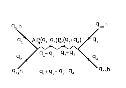
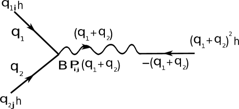
Figure 4: Vertices for the Feynman diagrams. (left)$\frac{A}{4}(P_{ij}\nabla_{i}h\nabla_{j}h)^{2}$; (right)$B(\nabla^{2}h)(P_{ij}\nabla_{i}h\nabla_{j}h)$.

After this perturbative step, we rescale lengths, with ${\bf r}=r{}^{\prime}e^{\ell}$, so as to restore the UV cutoff back to $\Lambda$. This is then followed by rescaling the long wave length part of the field $h({\bf q})=\zeta_{h}h^{\prime}({\bf q}^{\prime})$; $\zeta_{h}=b^{(d+4-\eta)/2}$, $\eta$ being the anomalous dimension of $h$, which we will choose to produce fixed points.

We restrict ourselves to a one-loop order renormalization group (RG) calculation. At this order (equivalently, to the lowest orders in $A$ and $B$), $\kappa$ receives two fluctuation corrections, each originating from non-zero $A$ and $B$, respectively; the relevant Feynman diagrams are given in Fig. 5.

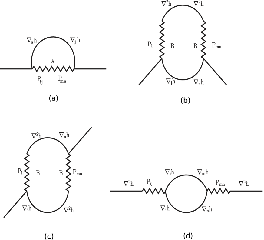
Figure 5: One-loop Feynman diagrams that contribute to the fluctuation corrections of $\kappa$.

Likewise, $A$ and $B$ are each renormalized at one-loop order by the graphs illustrated in Fig. 6 and Fig. 7 below, respectively.

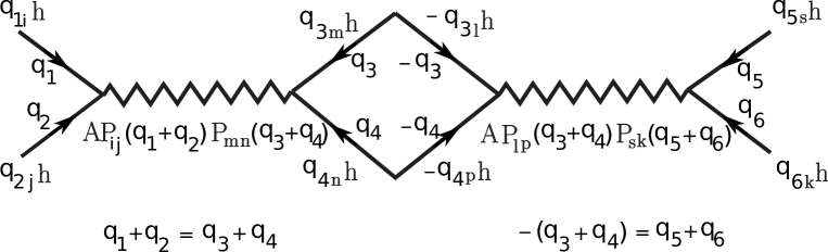
Figure 6: One-loop Feynman diagram for fluctuation corrections of $A$.

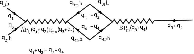
Figure 7: One-loop Feynman diagram for fluctuation corrections of $B$.

Many one loop graphs that are topologically possible, e.g., Fig. 11 and Fig. 12 in fact make vanishing contributions to $A$ and $B$, respectively. This is discussed in more detail in the Appendix, where we also calculate the graphs Figs. 5, 6, and 7 in detail. The result is the following recursion relations:

$$\frac{d\kappa}{dl}=\kappa\left[-\eta+g_{1}-\frac{5}{2}g_{2}\right]\,,$$ (II.34)

$$\frac{dA}{dl}=A\left[4-D-2\eta-\frac{g_{1}}{2}\right]\,,$$ (II.35)

$$\frac{dB}{dl}={B\over 2}\left[4-D-3\eta-g_{1}\right]\,,$$ (II.36)

$$\frac{dC_{0}}{dl}=(D-2+\eta)C_{0}+g_{2}\times{\cal O}(1)\,,$$ (II.37)

where we have defined two effective coupling constants,

$$g_{1}\equiv\frac{AK_{D}k_{B}T\Lambda^{-\epsilon}}{\kappa^{2}}\,\,\,,\,\,\,\,g_{2}\equiv\frac{B^{2}K_{D}k_{B}T\Lambda^{-\epsilon}}{\kappa^{3}}\,\,,$$ (II.38)

with $K_{D}=\frac{(D^{2}-1)S_{D}}{(2\pi)^{D}D(D+2)}$, where $S_{D}$ is the surface hyper-area of a D-dimensional sphere of unit radius, and $\epsilon\equiv 4-D$. We have not calculated the precise value of the ${\cal O}(1)$ constant in (II.37), as it affects none of the physics.

The recursion relations (II.34-II.37) can be combined into a closed set of recursion relations for the dimensionless couplings $g_{1}$ and $g_{2}$:

$$\frac{dg_{1}}{dl}=g_{1}[\epsilon-\frac{5g_{1}}{2}+{5}g_{2}],$$ (II.39)

$$\frac{dg_{2}}{dl}=g_{2}[\epsilon-4g_{1}+{{15\over 2}}g_{2}]\,.$$ (II.40)

While we have derived these recursion relations to lowest order in $g_{1}$ and $g_{2}$, certain features of them are exact. These are: first, that the recursion relations for $g_{1}$ and $g_{2}$ are completely independent of the value of $C$. This is because $C$ does not enter the propagator, since it is a surface term, and is not a coefficient of a higher than harmonic term. Therefore, it does not affect the renormalization of the remaining model parameters. Second, the recursion relation (II.37) for $C$ becomes exact when $g_{2}\rightarrow 0$, because, once $g_{2}=0$ (which requires $\chi=0$), the Hamiltonian (except for $C$ itself) is completely inversion-symmetric, and, hence, contains no anharmonic terms that can generate an inversion-asymmetric term like $C$.

The RG flows implied by the recursion relations (II.39, II.40) are illustrated in Fig. (8). There are only two fixed points in the physical quadrant $g_{1,2}>0$: an unstable Gaussian fixed point at $g_{1}=g_{2}=0$, and a stable fixed point

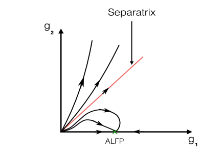
Figure 8: (Color online) Schematic flow lines in the $g_{1}-g_{2}$ plane implied by the recursion relations (II.39, II.40). The (green) cross marks the only stable FP ($g_{1}=2\epsilon/5,g_{2}=0$). The thick red curve is the separatrix ${g_{2}={3g_{1}\over 5}}$ between the region controlled by the stable Aronovitz-Lubensky fixed point (“ALFP”) Aronovitz and Lubensky (1988) (corresponding to a spiral membrane) and the region in which flows run off towards infinity. We believe the membrane is crumpled in this region.

$$g_{1}=2\epsilon/5,\,g_{2}=0\,.$$ (II.41)

Since we derived our RG recursion relations perturbatively assuming $g_{1}$ and $g_{2}$ were small, this result for the fixed point can only be trusted if $\epsilon=4-D\ll 1$. This is, of course, just the usual logic of the $\epsilon$-expansion Wilson (1975). While we therefore do not expect our results to be quantitatively reliable all the way down to D=2, where $\epsilon=2$, we do expect the topology and general features of the flows to remain the same. In particular, we expect the long-wavelength physics of the membrane, for length scales large compared to all microscopic lengths, but much less than the length scale $L_{H}$ on which the membrane starts having self-avoidance interactions with itself, to continue to be controlled by a fixed point at which $g_{2}=0$. Because $g_{2}=0$ at this fixed point, asymmetry is irrelevant (in a scaling/RG sense) in the phase that fixed point controls (i.e., for all systems whose “bare” or initial $g_{1}(\ell=0)$, $g_{2}(\ell=0)$ lie in the basin of attraction of this stable fixed point). Of course, this statement will cease to be true once the length scale under consideration grows to $L_{H}$, because at larger length scales the behavior of the membrane will be radically altered by self-avoidance interactions between successive turns of the spiral. But up to that length scale, asymmetry is irrelevant and the spontaneous curvature does not affect the physics of the membrane; therefore, the stable fixed point (II.41) must be the same as the fixed point of a symmetric membrane; i.e., it must be the Aronovitz-Lubensky  Aronovitz and Lubensky (1988) fixed point (which we will hereafter call the“ALFP”) (hence the label “ALFP” in Fig. (8)).

In particular, up to $L_{H}$, asymmetric membranes will exhibit the same anomalous elasticity of the bend modulus $\kappa$ as symmetric membranes. That is, the effective bend modulus $\kappa(\mathbf{q})$ at wavevector $\mathbf{q}$ grows without bound as $\mathbf{q}\to{\bf 0}$, diverging algebraically:

$$\kappa(\mathbf{q})=\kappa_{0}(q\xi_{{}_{NL}})^{-\eta}\,,$$ (II.42)

where $\kappa_{0}$ is the bare value of $\kappa$, and $\xi_{{}_{NL}}$ is a non-universal length at which fluctuation corrections to $\kappa_{0}$ start to dominate over $\kappa_{0}$. We will obtain this length from our recursion relations below. Furthermore, $\eta$ is a universal exponent given by the value of our previously defined rescaling exponent $\eta$ required to keep $\kappa(\ell)$ fixed upon renormalization. At the ALFP near $D=4$, $\eta=g_{1}=2\epsilon/5$. We do not, of course, expect this result to be quantitatively accurate all the way down to the physical case D=2, for which $\epsilon=2$. However, it is reasonable to assume that asymmetry remains irrelevant all the way down to D=2 (again, this is the usual reasoning applied to any $\epsilon$-expansion, which assumes that the structure of the RG flows does not change as one moves to larger $\epsilon$). Hence, the value of $\eta$ that holds for asymmetric membranes will be the same as that for symmetric membranes in D=2; the best estimate of that value is provided by Doussal and Radzihovsky (1992), which gives (I.5).

The analog of equation (II.42) in real space is the statement that the effective $\kappa$ on length scales $L$ obeys

$$\kappa(L)=\kappa_{0}\left({L\over\xi_{{}_{NL}}}\right)^{\eta}\,,$$ (II.43)

a result we will use later in our treatment of the spiral state.

We comment in passing that at this stable ALFP fixed point, on length scales small enough that the membrane looks flat and isolated, the renormalized correlations of the in-plane displacements $u_{i}({\bf q})$ can be obtained from (II.8). We obtain

$$\langle u_{i}({\bf q})u_{j}(-{\bf q})\rangle=k_{B}T\left[\frac{P_{ij}({\bf q})}{\mu(q)q^{2}}+\frac{L_{ij}({\bf q})}{(2\mu(q)+\lambda(q))q^{2}}\right]\,,$$ (II.44)

where the longitudinal projection operator

$$L_{ij}(\mathbf{q})\equiv\frac{q_{i}q_{j}}{q^{2}}$$ (II.45)

projects any vector along ${\bf q}$, and the renormalized elastic moduli $\mu(\mathbf{q})$ and $\lambda(\mathbf{q})$ are vanishing functions of wavevector $\mathbf{q}$:

$$\mu(\mathbf{q})\,,\lambda(\mathbf{q})\propto q^{\eta_{\mu}}$$ (II.46)

with

$$\eta_{\mu}=4-D-2\eta\,.$$ (II.47)

These results are identical in every respect, including the value of $\eta_{\mu}$, to those for symmetric tethered membranes Aronovitz and Lubensky (1988).

The non-linear length $\xi_{{}_{NL}}$ is simply the length scale at which $\kappa$ starts to acquire appreciable fluctuation corrections. Equivalently, it is the length scale on which one or both of the dimensionless non-linear couplings $g_{1,2}$ become of ${\cal O}(1)$. If the bare values $g^{0}_{1,2}$ of these couplings are both much less than $1$, then this length scale can be quite large. We will now estimate $\xi_{{}_{NL}}$ for the case in which the bare $g_{1,2}^{0}$ lie below the separatrix (II.55), and both are $\ll 1$.

Initially- that is, at renormalization group time $\ell=0$- the non-linear terms in the recursion relations (II.39) and (II.40) are negligible. Indeed, they will remain so at non-zero $\ell$ until the larger of $g_{1,2}(\ell)$ gets to be of ${\cal O}(1)$. Thus, up to the value $\ell_{1}$ of $\ell$ at which this happens, the recursion relations in D=2 (where $\epsilon=4-D=2$) reduce to:

$$\frac{dg_{1}}{dl}=2g_{1}\,,$$ (II.48)

$$\frac{dg_{2}}{dl}=2g_{2}\,,$$ (II.49)

whose solution is trivially

$$g_{1,2}(\ell)=g^{0}_{1,2}e^{2\ell}\,.$$ (II.50)

We can determine the value $\ell_{1}$ of $\ell$ at which the non-linearities become important by equating the larger of these to 1. This implies

$$e^{\ell_{1}}={\rm min}\left({1\over\sqrt{g^{0}_{1,2}}}\right)\,.$$ (II.51)

The non-linear length $\xi_{{}_{NL}}$ is just the length scale which, after precisely this much RG “time”, is rescaled to the inverse UV cutoff $\Lambda^{-1}$. This implies

$$\xi_{{}_{NL}}=\Lambda^{-1}e^{\ell_{1}}=\Lambda^{-1}{\rm min}\left({1\over\sqrt{g^{0}_{1,2}}}\right)\,.$$ (II.52)

Using equation (II.38) for $g_{1}$, with the parameters $\kappa$ and $A$ replaced by their bare values $\kappa_{0}$ and $A_{0}$ to obtain the bare value $g_{1}^{0}$ of $g_{1}$, and assuming that $g_{1}^{0}\gtrsim g_{2}^{0}$ (a condition which we’ll show below applies throughout the spiral phase), so that $g_{1}^{0}$ is the parameter that determines $\xi_{{}_{NL}}$, we obtain

$$\xi_{{}_{NL}}=\Lambda^{-1}e^{\ell_{1}}=\Lambda^{-1}\kappa_{0}\sqrt{1\over A_{0}K_{D}k_{B}T}\Lambda^{\epsilon\over 2}=\kappa_{0}\sqrt{1\over A_{0}K_{2}k_{B}T}\,,$$ (II.53)

where in the last equality we have specialized to the physical case D=2, for which $\epsilon\equiv 4-D=2$.

The above discussion, and, in particular, equations (II.42) and (II.43), apply to all membranes whose bare parameters lie in the regime that flows upon renormalization into the symmetric ALFP fixed point. However, not all bare parameters do so. To see this, consider the evolution of the ratio $\frac{g_{2}}{g_{1}}$. The flow equations (II.39) and (II.40) imply

$$\frac{d}{dl}\ln\left(\frac{g_{2}}{g_{1}}\right)=\frac{1}{g_{2}}\frac{dg_{2}}{dl}-\frac{1}{g_{1}}\frac{dg_{1}}{dl}=\frac{{5}}{2}g_{2}-{3\over{2}}g_{1}\,.$$ (II.54)

It is clear from this that if

$$g_{2}={{3\over 5}}g_{1}\,,$$ (II.55)

initially, this equality will continue to hold upon renormalization. Thus points on the locus (II.55) can not flow into the ALFP; indeed, they keep flowing out (to larger $g_{1,2}$) until they leave the regime of validity of our perturbation theory. Points above this locus can obviously not reach the ALFP either, since to do so, they would have to cross the locus (II.55), which they cannot do, since flow lines cannot cross. Therefore, the locus (II.55) acts as a separatrix between flows that go into the ALFP, which, as we have just discussed, imply scaling like symmetric membranes up to the length scale $L_{H}$, and those which instead flow out of the regime of validity of our perturbation theory, which will behave differently.

What is this different behavior? Since the flows in this regime lead out of the region of validity of our perturbation theory, we can only speculate. We will guide this speculation by the assumption that symmetric membranes have a continuous crumpling transition. This implies that at larger $g_{1}$ on the $g_{1}$ axis, there must be an unstable fixed point controlling this crumpling transition. If we now consider the full flows of an asymmetric membrane in the two dimensional parameter space $(g_{1},g_{2})$ and connect this putative flow on the $g_{1}$ axis with our flows near the origin in the simplest possible way (i.e., one that does not involve introducing any new fixed points), then we are lead to Fig. (9). This is an “Occam’s razor” argument: Fig. (9) is the simplest flow topology that incorporates our known flows for small $g_{1,2}$ and $\epsilon$ with the putative flows that allow for a continuous crumpling transition for a symmetric membrane.

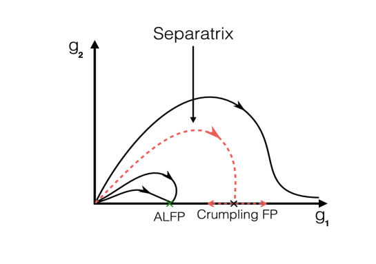
Figure 9: Conjectured “Occam’s razor” global RG flows in the $g_{1}-g_{2}$ plane.

Note that this conjectured topology implies the separatrix flows to the crumpling fixed point; this implies that if we vary membrane parameters (including temperature) in such a way that the bare $g_{1,2}$ cross the separatrix, the membrane will crumple.

This interpretation of the separatrix as the crumpling threshold is supported by the observation that the underlying reason for the runaway RG flows on and above the separatrix is that the bend modulus $\kappa$ is being driven downwards by the $-{5\over 2}g_{2}$ term in its recursion relation. If $\kappa$ is driven to zero by this term, $g_{1}$ and $g_{2}$ both diverge. If $\kappa$ is driven to negative values by this term, the membrane will clearly crumple.

We cannot, of course, follow this flow of $\kappa$ from positive to negative values, since the divergence of $g_{1}$ and $g_{2}$ as $\kappa\to 0$ invalidates our perturbative RG calculation. But the structure of the recursion relations just discussed strongly suggests that the separatrix is the crumpling boundary, which supports our conjectured topology Fig. (9) for the global RG flows.

Note that this crumpling is occurring in a regime in which the bare bend modulus $\kappa_{0}$ given by eqn. (II.5) is positive; this is an anharmonic crumpling mechanism, beyond the harmonic theory of crumpling we developed in section (II.2). Note also $\kappa(\ell)>0$ at small enough $\ell$; this implies small enough membranes will not crumple, which in turn implies our two length scale regimes in fig. (2). We will discuss this in more detail in section (III.3).

III $L\gg L_{H}$: Global membrane structure, the spiral state, and crumpling revisited

III.1 The spiral state for $T=0$

Since the $A$ term is long-ranged, and a perfect square, this implies that, in the absence of the $B$ term, the lowest energy configurations of the membrane will have zero Gaussian curvature. This is why the ”spiral” state of the membrane, that results from the competition between the spontaneous curvature, bending energy and excluded volume effects, curls in only one direction. We now heuristically argue that at $T=0$, the $B$-term, even when nonzero, is always irrelevant in the thermodynamic limit, making the spiral phase the only ground state at $T=0$. To show this, we make a rough estimate of the free energy ${\mathcal{F}}_{h}$ in (LABEL:free_energy_h_RS) in terms of Gaussian curvature $S$ and mean curvature $M$, both of which are assumed to be constant for simplicity. this gives

$${\mathcal{F}}_{h}^{\rm rough}={\kappa_{0}}L^{2}(M-\frac{C}{\kappa_{0}})^{2}+A_{0}L^{6}S^{2}+B_{0}L^{4}MS\,,$$ (III.1)

where we have ignored numerical factors of ${\cal O}(1)$, and logarithmic factors, in this rough estimate, and have crudely estimated the kernels of the $A_{0}$ and $0$-terms in ${\mathcal{F}}_{h}$ (LABEL:free_energy_h_RS) as $L^{2}$ and $L^{0}$ respectively. Minimizing ${\mathcal{F}}_{h}^{\rm rough}$ with respect to the Gaussian and mean curvatures $S$ and $M$ yields, again ignoring factors of ${\cal O}(1)$,

$${-\kappa_{0}}L^{2}(M-\frac{C}{\kappa_{0}}) = B_{0}L^{4}S\,,$$ (III.2)

$$-A_{0}L^{6}S = B_{0}L^{4}M\,.$$ (III.3)

These are readily solved to give

$$M = {C\over\kappa_{0}-{B_{0}^{2}\over A_{0}}}\,,$$ (III.4)

$$S = -{B_{0}C\over A_{0}\kappa_{0}-B_{0}^{2}}{1\over L^{2}}\,.$$ (III.5)

Thus in the thermodynamic limit $L\rightarrow\infty$, $S$ vanishes and the ground state must be a state given by $M=C/\kappa_{0}\equiv 2r_{0}$ with zero Gaussian curvature, where $r_{0}$ is given by (I.2); see also Appendix Appendix VIII: Demonstration that the hole in the middle for $T=0$ is negligibly small. This implies that the membrane must bend only in one direction; the inversion symmetry breaking $B$ term does not alter this conclusion. For a square membrane, the bent direction is spontaneously chosen; for a rectangular membrane it is energetically profitable to roll up along the longer direction.

The above argument assumes that the bend modulus $\kappa_{0}$ is positive. As we have seen, there are regions of the parameter space for which this is not true: specifically, $\chi^{2}>\chi_{U}^{2}$. In that case, the membrane wants to maximize both its Gaussian and its mean curvatures, which it does by crumpling.

Returning now to the case $\kappa_{0}>0$, we note that, while it will not affect the conclusion that the membrane will bend in only one direction, self-avoidance will radically alter the radius of curvature in the single bent direction. This becomes obvious once we note that, were the membrane to roll up into a cylinder with radius $r_{0}$, its volume $V$ would be $V\sim r_{0}^{2}L<<L^{2}a$, where $L^{2}a$ is the volume of the material of the membrane itself. Therefore, such a tightly rolled membrane would be extremely self-overlapping. To avoid this, it must wrap less tightly. On the other hand, it energetically prefers to be wrapped as close the optimal radius of curvature $r_{0}$ as possible. It can do this by wrapping as tightly as possible in one direction without overlapping. The structure that results can be seen by imagining starting with flat membrane, and wrapping it from one end at spontaneous curvature. When one has rolled up a length $2\pi r_{0}$ of membrane, the end of the membrane encounters the remainder (i.e., the as yet unrolled up portion) of the membrane. This part therefore cannot wrap at $r_{0}$, so it instead wraps up as tightly as it can, which is readily seen to be a radius of curvature $r_{0}$ plus $a$. This continues until this section is rolled up into the remainder of membrane; now radius of curvature becomes $r_{0}+2a$. Each successive turn is therefore spaced by the membrane thickness $a$ from the previous one, leaving just enough room for one layer. This is clearly the tightest wrapping allowed by self-avoidance. This structure we’ve just described is a spiral of Archimedes (I.1), with a hole in the center of radius $r_{0}$. In appendix VI, we show that the radius of this hole is indeed ${\cal O}(r_{0})$; in fact, it is $r_{0}$, which is therefore negligible for $L>>r_{0}$. F

III.2 The spiral state for $T\neq 0$

We now turn to the effects of thermal fluctuations on the spiral phase. This requires studying the system at larger scales $L\gg L_{H}$. That a large enough asymmetric membrane takes the form of a double spiral (see Fig. 1), should still hold for $T>0$. Thermal fluctuations, however, considerably affect the form of the spiral by giving rise to a longer ranged ”Helfrich repulsion”Helfrich (1978) that has its origin in excluded volume interactions and important over scales $L\gg L_{H}$. This opens the spiral up. When such fluctuations are important (as they always will be for a sufficiently large membrane), the form of the spiral changes to a power law, as we show below. The Helfrich interaction energy at $T>0$ was first derived for fluid membranes in Helfrich (1978), and was calculated for tethered membranes in Toner (1990).

We review this calculation here. Up to the length scale $L_{H}$ at which the membrane starts interacting with neighboring turns of the spiral, it acts like a free membrane, as treated in the last subsection. Therefore, the contribution of fluctuations on shorter length scales to the total mean squared height fluctuations $\left<h(\mathbf{r})^{2}\right>$ can be calculated precisely as one would for a free membrane, but with an infrared cutoff (i.e., minimum wavenumber) given by the inverse of $L_{H}$. This implies:

$$\left<h(\mathbf{r})^{2}\right>=\int_{q>q_{m}}{d^{2}q\over(2\pi)^{2}}\,\left<|h(\mathbf{q})|^{2}\right>\,,$$ (III.6)

with the infrared cutoff $q_{m}\sim 1/L_{H}$. Our RG analysis showed that, at small $\mathbf{q}$, which is readily seen to be the regime of wavevector that dominates the integral in this expression (III.6),

$$\left<|h(\mathbf{q})|^{2}\right>={k_{B}T\over\kappa(\mathbf{q})q^{4}}\,,$$ (III.7)

with the effective, renormalized bend modulus $\kappa(\mathbf{q})$ given by (II.42), with, we recall, the anomalous elasticity exponent $\eta$ precisely the same as that for symmetric membranes, in the regime in which our RG flows go into the symmetric ALFP in figure (9). Since the integral over $\mathbf{q}$ in (III.6) is dominated by small wavenumbers $q$, we obtain

$$\left<h(\mathbf{r})^{2}\right>={k_{B}T\over\kappa_{0}}\xi_{NL}^{\eta}L^{2-\eta}_{H}\times{\cal O}(1)\,,$$ (III.8)

where we have absorbed our uncertainty about the precise value of the infra-red cutoff into the ${\cal O}(1)$ factor. We can now obtain ${L_{H}}$ by roughly equating this mean squared fluctuation to the square of the distance $d$ to the next turn, since a patch of membrane of this size is just big enough to fluctuate enough to contact the turn above it. This gives

$$\left<h(\mathbf{r})^{2}\right>={k_{B}T\over\kappa_{0}}\xi_{NL}^{\eta}L^{2-\eta}_{H}\times{\cal O}(1)=d^{2}\times{\cal O}(1)\,,$$ (III.9)

which is trivially solved for ${L_{H}}$:

$${L_{H}}=\left({\kappa_{0}\over k_{B}T}\right)^{1/(2-\eta)}\xi_{NL}^{-\eta/(2-\eta)}d^{2/(2-\eta)}\times{\cal O}(1)\,.$$ (III.10)

With this result for the typical distance ${L_{H}}$ between points of contact between neighboring membranes in hand, one can now argue Helfrich (1978) that each such contact causes a reduction in entropy, since the motion of the membrane is restricted by self-avoidance at these points. Assuming this reduction is of ${\cal O}(1)$ for each contact implies that each contact costs a typical free energy of ${\cal O}(k_{B}T)$. Thus the total free energy cost per unit area is given by

$$\mathcal{U}_{H}(d)={k_{B}T\over L^{2}_{H}}\times{\cal O}(1)=\left({k_{B}T\over\kappa_{0}}\right)^{2}A_{0}\left({w\over d}\right)^{\gamma}\times{\cal O}(1),$$

(III.11)

where

$$\gamma\equiv{4\over 2-\eta}\,,$$ (III.12)

and we have used our earlier expression (II.53) for $\xi_{NL}$ to write this expression entirely in terms of the bare values $\kappa_{0}$ and $A_{0}$ of $\kappa$ and $A={4\mu(\mu+\lambda)\over 2\mu+\lambda}$, and the length $w$ is given by

$$w=\sqrt{\kappa_{0}\over A_{0}}\,.$$ (III.13)

In a simple model of the membrane as an elastic continuum one would obtain Landau and Lifshitz (1970) $A_{0}\sim\mu_{3d}a$ and $\kappa_{0}\sim\mu_{3d}a^{3}$, which imply $w=a\times{\cal O}(1)$, where $a$ is the membrane thickness.

Now let us consider the effects of this interaction on a spiral membrane. We first need to relate the distance $d$ between successive turns of the spiral to its radius profile $r(s)$, where $s$ is arc-length along the spiral from the center. Note that in general, unlike the Archimidean spiral, this distance will vary with arc-length $s$ along the spiral.

If the spiral is very tightly wound, (and we will verify a posteriori that it is), so that the angle between the spiral and the radius drawn from the center of the spiral to the point in question is close to $90\degree$, then the spacing $d(s)$ of successive turns of the membrane at a distance $s$ along the membrane is the difference between $r(s=s_{A})$ and $r(s=s_{B})$, as illustrated in Fig. 10.

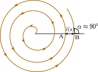
Figure 10: (Color online) Cross section of a single spiral at $T>0$.

Note that $s_{B}-s_{A}$ is very nearly $2\pi r(s)$ for a tightly wound spiral (i.e., the path between $A$ and $B$ is nearly a circle of radius $r(s_{A})$). Furthermore, if ${dr\over ds}$ varies slowly with $s$ (which we will again verify a posteriori), so that it is nearly constant between $A$ and $B$, then we can say that the spacing between successive turns of the membrane is given by

$$d(s_{A})\approx r(s_{B})-r(s_{A})\approx 2\pi r(s_{A}){dr\over ds}|_{s=s_{A}}\,,$$

(III.14)

or more generally

$$d(s)\equiv 2\pi r(s){dr\over ds}\,.$$ (III.15)

The structure of the spiral can now be determined by balancing this Helfrich interaction against the two other terms in the free energy: the spontaneous curvature energy $C/R$ (where $R$ is the mean curvature), and the bending energy. The latter must be calculated using the renormalized value of $\kappa$. In doing so, we must recognize that the anomalous length dependence (II.43) of $\kappa$ is cut off for length scales $L\gtrsim L_{H}$, since the height fluctuations stop growing at that point, due to the self-avoidance interactions with the next turn of the spiral. This implies that $\kappa$ becomes length scale independent larger length scales. Matching this constant onto the value of $\kappa(L)$ at the largest $L$’s for which the elasticity is still anomalous, namely $L\sim L_{H}$, implies that this constant value of $\kappa$ on larger length scales is given by

$$\kappa(L>L_{H})\sim\kappa(L\sim L_{H})\sim\kappa_{0}\left({L_{H}\over\xi_{{}_{NL}}}\right)^{\eta}\,.$$ (III.16)

Since $L_{H}$ increases with $d(s)$, where $d$ is the distance to the next turn of the membrane, the fact that $d(s)$ depends on distance $s$ along the spiral implies that $L_{H}(s)$ will as well. Hence, through, (III.16), so will $\kappa$.

The spontaneous curvature coefficient $C$, on the other hand, exhibits no such anomaly, since, as we noted in our RG discussion in the last section, its graphical corrections vanish when $g_{2}$ does, as it does in the region of parameter space we are considering here.

The final ingredient we need to calculate the bend and spontaneous curvature energies is an expression for the mean curvature $R(s)$, which will also depend on distance $s$ along the spiral. For a very tightly wound spiral, this is simply $r(s)$ itself.

We can summarize all of the above reasoning in the following expression for the energy of a spiral:

$$E=2L_{||}\int^{L_{\bot}/2}_{0}ds\left[-{C\over r(s)}+{\kappa_{0}\over{2}r^{2}}\left({L_{H}(s)\over\xi_{{}_{NL}}}\right)^{\eta}+{\mathfrak{D}\over[r{dr\over ds}]^{\gamma}}\right],$$

(III.17)

where

$$\mathfrak{D}=\left({k_{B}T\over\kappa_{0}}\right)^{2}{A_{0}w^{\gamma}\times{\cal O}(1)}\,.$$ (III.18)

We will now obtain the structure $r(s)$ of the spiral by minimizing this free energy. In doing so, we will assume, and verify a posteriori, that the bending energy is negligible for a sufficiently large spiral. Doing so, the Euler-Lagrange equation for $r(s)$ obtained by minimizing the energy (III.17) over $r(s)$ is

$$-\gamma\mathfrak{D}{d\over ds}\left[{1\over r^{\gamma}({dr\over ds})^{\gamma+1}}\right]={C\over r^{2}}-{\gamma\mathfrak{D}\over r^{\gamma+1}({dr\over ds})^{\gamma}}\,.$$ (III.19)

Formidable though this equation looks, it is easily solved by the ansatz:

$$r=s_{0}\left({s\over s_{0}}\right)^{\alpha}\,,$$ (III.20)

which, when inserted into the Euler-LaGrange equation (III.19) yields

$$\Gamma_{1}(\alpha,\gamma)\mathfrak{D}s_{0}^{[(\alpha-1)(2\gamma+1)]}s^{-[\alpha(2\gamma+1)-\gamma]}=Cs_{0}^{2(\alpha-1)}s^{-2\alpha}$$ (III.21)

where we have defined the unimportant, ${\cal O}(1)$ constant

$$\Gamma_{1}(\alpha,\gamma)=\gamma\alpha^{-(\gamma+1)}[2(\gamma+1)\alpha-\gamma-1]\,.$$ (III.22)

Balancing powers on both sides of this equation determines the shape exponent $\alpha$:

$$\alpha={\gamma\over 2\gamma-1}\,,$$ (III.23)

while equating the constant prefactors determines $s_{0}$:

$$s_{0}=\left(\mathfrak{D}\over C\right)^{1\over\gamma-1}\Gamma_{2}(\gamma)\,,$$ (III.24)

where we have defined yet another unimportant ${\cal O}(1)$ constant

$$\Gamma_{2}(\gamma)=\left[(\gamma+1)\left({2\gamma-1\over\gamma}\right)^{\gamma}\right]^{1\over\gamma-1}\,,$$ (III.25)

which is a monotonically decreasing function of $\gamma$ over the entire allowed range $2<\gamma<4$, and hence bounded above by $\Gamma_{2}(2)=6.75$ exactly, and below by $\Gamma_{2}(4)\approx 3.606125$. If we take the canonical value of $\eta={4\over 1+\sqrt{15}}$, which implies $\gamma\approx 3.39$, we get $\Gamma_{2}\approx 3.95655$.

Using our expression (III.12) for $\gamma$ in terms of $\eta$ in (III.23) gives

$$\alpha={4\over 6+\eta}.$$ (III.26)

Using these expressions (III.24) and (III.26) in our ansatz (III.20) for $r(s)$ completely specifies the shape of the spiral. To express that shape in more familiar polar coordinates, we use the fact that, for a tightly wound spiral,

$${ds\over d\theta}=\sqrt{r^{2}+\left({dr\over d\theta}\right)^{2}}\approx r\,.$$ (III.27)

Using Eq. (III.20), this can be integrated to give

$$\left({s\over s_{0}}\right)^{1-\alpha}=(1-\alpha)\theta,$$ (III.28)

with the boundary condition $\theta=0,\,s=0$. Thus solving for $s(\theta)$:

$$s=s_{0}((1-\alpha)\theta)^{1/(1-\alpha)}\,.$$ (III.29)

Using Eq. (III.29) in (III.20), we get $r(\theta)$ as a function of $\theta$:

$$r(\theta)=R_{0}\theta^{\nu},$$ (III.30)

where

$$\nu={\alpha\over(1-\alpha)}={4\over 2+\eta}{\approx 4-{2\over 3}\sqrt{15}\approx 1.418}\,,$$ (III.31)

and

$$R_{0}\equiv s_{0}(1-\alpha)^{\nu}\,.$$ (III.32)

The numerical estimates of the exponents are based on the theoretical estimate of $\eta$ for the flat phase of asymmetric membranes:

$$\eta={4\over 1+\sqrt{15}}\approx.821$$ (III.33)

obtained by Radzihovsky and LeDoussalDoussal and Radzihovsky (1992).

The above results are those summarized in equations (I.3), (I.4), and (I.5) of the introduction.

Using our earlier result (III.24) for $s_{0}$ in (III.32), we find that the scale length $R_{0}$ exhibits universal scaling with temperature and other parameters, which can also be related exactly to the exponent $\eta$; we find

$$R_{0}=\left[(k_{B}T)^{2(2-\eta)}\kappa_{0}^{2(\eta-1)}A_{0}^{-{\eta}}C^{(\eta-2)}\right]^{1/(2+\eta)}\times{\cal O}(1)\,,$$

(III.34)

where we remind the reader that $\kappa_{0}=\kappa(l=0)$ is the ”bare” bend modulus and $A_{0}\equiv\frac{4\mu_{0}(\mu_{0}+\lambda_{0})}{2\mu_{0}+\lambda_{0}}>0$, with $\mu_{0}$ and $\lambda_{0}$ the equally bare Lame’ coefficients. Here, by “bare”, we mean the values these parameters have before being renormalized by thermal fluctuation effects. In deriving (III.34), we have used our expressions (III.18) for $D$ and (III.13) for $w$. This result (III.34) is precisely equation (I.6) of the introduction.

The total radius $R_{T}$ of the spiral regions also exhibits universal scaling, in this case with the spatial extent $L$ of the membrane, as may be obtained from (III.20) with $s=L$

$$R_{T}=R_{0}^{1-\alpha}L^{\alpha}\,.$$ (III.35)

It is straightforward to use these results to verify our three earlier a posteriori assumptions, which we remind the reader were:

1) that the spiral is “tightly wound”, in the sense that the angle between the spiral and the radius vector is close to $90$ degrees,

2) that ${dr\over ds}$ does not vary appreciably between successive turns of the spiral, and

3) that the bending energy is negligible compared to the Helfrich interaction and the spontaneous curvature energy.

Both of these results follow from the algebraic (i.e., power-law) form of the spiral. The angle $\phi$ between the radius vector and the spiral obeys

$$\tan\phi={d\theta\over d\ln r}\,.$$ (III.36)

Using our expression (III.20) for $r(s)$ in this expression, we see that

$$\tan\phi={\theta\over\nu}\,,$$ (III.37)

which is clearly $\gg 1$ after the first few turns (i.e., for $\theta\gg 2\pi$), since $\nu\approx 1.418$ is ${\cal O}(1)$. This implies that

$$\phi\approx{\pi\over 2}-{\nu\over\theta}\to{\pi\over 2}\,.$$ (III.38)

This completes our demonstration that the spiral is tightly wound. Turning next to the question of whether ${dr\over ds}$ varies appreciably over one turn of the spiral, we note that we can estimate the change in ${dr\over ds}$ over one turn as

$$\Delta\left({dr\over ds}\right)=\left({dr\over ds}\right)_{s+2\pi r}-\left({dr\over ds}\right)_{s}\approx 2\pi r{d^{2}r\over ds^{2}}\,.$$ (III.39)

Using (III.20) in this expression yields

$$\Delta\left({dr\over ds}\right)=2\pi\alpha(\alpha-1)\left({s\over s_{0}}\right)^{2(\alpha-1)}\to 0\,,$$ (III.40)

as $s\to\infty$, since $\alpha<1$.

Finally we turn to our third a posteriori assumption, that the bending energy is negligible compared to the Helfrich interaction and the spontaneous curvature energy.

The bending free energy density, as shown in (III.17), is

$$f_{\rm{bend}}={\kappa_{0}\over r^{2}(s)}\left({L_{H}(s)\over\xi_{{}_{NL}}}\right)^{\eta}\,.$$ (III.41)

Using our expression (III.10) for $L_{H}$ in terms of the spacing $d$ between successive turns of the membrane, and using (III.15) to relate $d(s)$ to $r(s)$, we find that

$$f_{\rm{bend}}=\Gamma_{B}r^{4(\eta-1)\over 2-\eta}\left({dr\over ds}\right)^{2\eta\over 2-\eta}\,,$$ (III.42)

where we have defined the constant

$$\Gamma_{B}\equiv\left({\kappa_{0}\over k_{B}T}\right)^{2\over 2-\eta}\xi_{{}_{NL}}^{-\left({2\eta\over 2-\eta}\right)}k_{B}T\,.$$ (III.43)

Now using our expressions (III.20) and (III.26) for $r(s)$ in (III.42), we find that

$$f_{\rm{bend}}\propto s^{\nu_{b}}\,,$$ (III.44)

where the exponent $\nu_{b}$ is given by

$$\nu_{b}={2(\eta-4)\over 6+\eta}\,.$$ (III.45)

Likewise, the spontaneous curvature free energy density $f_{C}\equiv-C/r(s)$ obeys

$$f_{C}\propto{1\over r(s)}\propto s^{-\alpha}=s^{-\left({4\over 6+\eta}\right)}\,.$$ (III.46)

Taking the ratio of the bending energy (III.44) to this, we find

$${f_{\rm{bend}}\over f_{C}}\propto s^{\nu_{bc}}\,,$$ (III.47)

where

$$\nu_{bc}={2(\eta-4)\over 6+\eta}+{4\over 6+\eta}={2(\eta-2)\over 6+\eta}\,.$$ (III.48)

Since $\eta<2$, this exponent $\nu_{bc}<0$. Therefore, as $s\to\infty$, the ratio of the bending energy to the spontaneous curvature energy vanishes, proving that it is, as we assumed, negligible for a sufficiently large membrane.

This completes our a posteriori verification of all three of the assumptions we used in deriving the form of the spiral.

We now argue that asymmetric tethered membranes in the spiral phase indeed display long range order. By long range order we mean predictability of the direction of the local normal ${\bf n}$ throughout the membrane, given its position at one point on the membrane, in the thermodynamic limit. This requires that the variance of the fluctuations $\delta\bf n$ of the local normal about its position at $T=0$ must be bounded in the thermodynamic limit. This is true for statistically flat symmetric tethered membranes, for which the local normals are all parallel to each other at $T=0$. For asymmetric tethered membranes at $T=0$, the normals are not parallel due to the spiral structure; nonetheless, they are uniquely determined by that spiral structure everywhere on the membrane. We now argue that the variance $\langle(\delta{\bf n})^{2}\rangle$ about this deterministic spiral structure is indeed finite in the spiral phase of asymmetric tethered membranes.

We begin by noting that $\langle(\delta{\bf n})^{2}\rangle$ gets contributions from two regimes of wavevectors:

(i) $q\gg L_{H}^{-1}$, on which the elasticity of the membrane looks like that of a symmetric membrane in isolation. Therefore, the contribution of fluctuations from this range of wavevector to $\langle(\delta{\bf n})^{2}\rangle$ is finite for the same reason - namely, the divergence of $\kappa(\mathbf{q})$ at long wavelengths- as for symmetric tethered membranes.

(ii) $q\ll L_{H}^{-1}$, on which the elasticity of the membrane looks like that of a bulk smectic A. For that range, the standard theory of smectic layer fluctuations impliesChaikin and Lubensky (2000) that

$$\langle(\delta{\bf n})^{2}\rangle=\int{d^{3}q\over(2\pi)^{3}}\,\,{k_{B}Tq_{\perp}^{2}\over(\tilde{B}q_{z}^{2}+Kq_{\perp}^{4})}\,.$$ (III.49)

Here, $\tilde{B}$ and $K$ are respectively the standard layer compression and layer bending elastic constants for smectics, which are related to $\kappa(L_{H})$: $K\sim\kappa(L_{H})/d$ and $\tilde{B}={\partial^{2}U_{H}\over\partial d^{2}}d\sim(k_{B}T)^{2}/(\kappa(L_{H})d^{3})$; and $q_{z}$ and $q_{\perp}$ are respectively the magnitudes of the components of the wavevector along and perpendicular to the direction locally perpendicular to the layers. The integral in (III.49) converges down to ${\bf q}=0$. Thus $\langle(\delta{\bf n})^{2}\rangle$ remains finite; this establishes that long range orientational order exists in the spiral phase.

The above analysis applies on length scales small compared to the local radius of the spiral. On longer length scales, the director simply follows the normal to the spiral.

III.3 Crumpling revisited

Having discussed the spiral phase, we turn now to the other region of parameter space, namely that which flows away from the ALFP, and towards negative $\kappa$. While we cannot follow these flows all the way to $\kappa=0$ (since both $g_{1,2}$ diverge there, so that our perturbation theory breaks down), we suspect that this signals crumpling of large membranes. This region of parameter space therefore corresponds to the crumpled phase. For $\epsilon=4-d\ll 1$, which is the region in which our perturbative RG is accurate, this is the region in Fig. (2) lying above the separatrix $g_{2}=3g_{1}/5$. For the physical case $\epsilon=2$, it seems reasonable to assume that there continues to be a separatrix which, for small $g_{1,2}$, is a straight line $g_{2}=\rho g_{1}$ of universal slope $\rho={\cal O}(1)$, although since $\epsilon=2$ we cannot calculate the universal constant $\rho$.

The range of bare asymmetry parameter $\chi$ in our original model (II.1) that we are now discussing is $\chi_{{}_{{}_{L}}}^{2}<\chi^{2}<\chi_{{}_{U}}^{2}$, where the upper bound follows because we are considering positive $\kappa_{0}$ in equation (II.5), while the lower bound follows from assuming that we are above the separatrix, which implies, for small bare $g^{0}_{1,2}$, that $g^{0}_{2}/g^{0}_{1}>\rho$. Using our earlier expressions (II.38) for $g_{1,2}$, we see that this implies

$$\chi^{2}>{\rho\kappa^{\prime}(2\mu_{0}+\lambda_{0})\over\rho+{\mu_{0}\over\mu_{0}+\lambda_{0}}}={\chi_{{}_{U}}^{2}\over 1+{\mu_{0}\over\rho(\mu_{0}+\lambda_{0})}}\equiv\chi_{{}_{{}_{L}}}^{2}\,,$$ (III.50)

where in the equality we have used our result (II.6) for $\chi_{{}_{U}}^{2}$. Note that, reassuringly, we always have $\chi_{{}_{{}_{L}}}^{2}<\chi_{{}_{U}}^{2}$, since $\rho$, $\mu_{0}$, and $\mu_{0}+\lambda_{0}$ are all positive, the latter two positivities being required for stability.

For $\chi$’s in the range $\chi_{{}_{{}_{L}}}^{2}<\chi^{2}<\chi_{{}_{U}}^{2}$, the membrane can remain uncrumpled if it is sufficiently small. This is because the bare value $\kappa(\ell=0)=\kappa_{0}=\kappa^{\prime}-\frac{\chi_{0}^{2}}{2\mu_{0}+\lambda_{0}}$ is positive in this range of $\chi$’s, and can stabilize orientational order, and thereby prevent crumpling, on length scales short enough that the renormalized $\kappa$ is not yet driven to $0$ by anharmonic fluctuation effects. This implies that the membrane can avoid crumpling if some new physics beyond the purely elastic model (II.1) intervenes on some new length scale $L_{\rm new}$ smaller than the orientational correlation length $\xi$, which is given by

$$\xi=\Lambda^{-1}e^{\ell_{v}}\ ,$$ (III.51)

with $\ell_{v}$ defined as the RG “time” at which $\kappa(\ell_{v})=0$. (Here we have used the usual relation $L(\ell)=\Lambda^{-1}e^{\ell}$ between renormalization group “time” $\ell$ and length scale $L$.)

We can therefore calculate the maximum length $L_{c}$ that a membrane can have while still remaining uncrumpled by calculating the orientational correlation length $\xi$, and the “new physics” length scale $L_{\rm new}$ (which will depend on the membrane length $L_{m}$), and then equating the two.

We will begin by calculating $\xi$ in the limit $\chi^{2}\rightarrow\chi_{{}_{U}}^{2}$ from below using the recursion relations (II.37). In this limit, since the bare parameters $g^{0}_{1}\propto 1/\kappa_{0}^{2}$ and $g^{0}_{2}\propto 1/\kappa_{0}^{3}$, $g^{0}_{2}$ diverges faster than $g^{0}_{1}$ as $\kappa_{0}\rightarrow 0$; hence, $g^{0}_{2}\gg g^{0}_{1}$ as $\chi^{2}\rightarrow\chi_{{}_{U}}^{2}$ from below. The recursion relation (II.54) for the ratio ${g_{2}(\ell)\over g_{1}(\ell)}$ then implies that in this region of parameter space, $g_{2}(\ell)\gg g_{1}(\ell)$ for all $\ell$, since their ratio grows everywhere above the separatrix. The value $\ell_{v}$ of $\ell$ at which $\kappa(\ell)$ vanishes is the same as the value of $\ell$ at which $g_{2}(\ell)$ diverges, since, as can be seen from its definition, $g_{2}(\ell)\rightarrow\infty$ as $\kappa(\ell)\rightarrow 0$. This value can be approximated, for small bare $g_{2}^{0}$, by $\ell_{1}$, the value of $\ell$ at which $g_{2}(\ell=\ell_{1})={\cal O}(1)$, since, once $g_{2}(\ell)$ gets to be of ${\cal O}(1)$, only a finite, ${\cal O}(1)$ further renormalization group time $\delta\ell$ is required for $g_{2}(\ell)$ to grow from ${\cal O}(1)$ to $\infty$. This statement can be verified directly from the recursion relation (II.40) for $g_{2}$ which, in the limit $g_{1}(\ell)\ll g_{2}(\ell)$ (a limit which we showed above holds for all $\ell$ in the limit $\chi^{2}\rightarrow\chi_{{}_{U}}^{2}$ from below), can be solved analytically, yielding

$$\ell={1\over\epsilon}\ln\left[\left({g_{2}(\ell)\over\epsilon+15g_{2}(\ell)/2}\right)\left({\epsilon+15g_{2}^{0}/2\over g_{2}^{0}}\right)\right]\ .$$ (III.52)

Evaluating this for the physical case $\epsilon=2$ in the limit $g_{2}^{0}\ll 1$ with $g_{2}(\ell_{1})=1$ gives

$$\ell_{1}={1\over 2}\left[\ln\left({2\over g_{2}^{0}}\right)-\ln(19/2)\right]\,$$ (III.53)

and

$$\ell_{v}={1\over 2}\ln\left({2\over g_{2}^{0}}\right)\,,$$ (III.54)

where in (III.54) we have used the fact that $g_{2}(\ell_{v})=\infty$, since $\kappa(\ell_{v})=0$, by definition. As claimed, these two values of $\ell$ differ by an amount of ${\cal O}(1)$. Of course, we do not actually know the precise value of this ${\cal O}(1)$ constant, since our recursion relations (II.39) and (II.40) are not accurate for $g_{2}\gg 1$. However, that the difference $\ell_{0}-\ell_{1}$ is of ${\cal O}(1)$ is clear, provided that the flows do not pass too close to the putative strong coupling fixed point in figure (9).

Using the result (III.54) for $\ell_{v}$ in our expression (III.51) for the orientational correlation length gives

$$\xi=\Lambda^{-1}\sqrt{1\over g^{0}_{2}}\times O(1)={1\over B_{0}}\sqrt{\kappa_{0}^{3}\over k_{B}T}\times O(1)\ ,$$ (III.55)

where in the second equality we have used our expression (II.38) for $g_{2}$, evaluated with the bare values $B_{0}$ and $\kappa_{0}$ of the parameters $B$ and $\kappa$, to evaluate $g_{2}^{0}$.

We now turn to the calculation of the length scale $L_{\rm new}$ beyond which new physics not included in the elastic model (II.1) can intervene to prevent crumpling before this length scale is reached. We have already discussed one such piece of physics: self-avoidance. The associated length scale $L_{H}$ is the typical distance between successive contacts between neighboring turns of the spiral, and can cut off any tendency to crumpling in the spiral sections of the membrane. But as inspection of Fig. (1) makes clear, there is one section of the membrane for which this cutoff cannot work: the straight section connecting the two oppositely returning spirals. This section has no neighbors, because it lies outside both spirals. It is therefore the section of the membrane that will crumple first, thereby inducing crumpling of the rest of the membrane.

This straight, “connecting” section of the membrane is stabilized by surface tension, which arises because that section of the membrane could lower its energy by “rolling up” into one or the other of the spiral sections it connects (since it should thereby be closer to the optimal spontaneous curvature). It is not rolled up, of course, because the other spiral pulls it equally hard in the opposite direction. These two pulls create a non-zero surface tension $\sigma$, whose magnitude should be comparable to the Helfrich interaction in the outermost turn of the spiral, since it is the balance between that interaction, which works to open the spiral, and the spontaneous curvature term, which tightens, that sets the scale of the energy of those outermost turns of the membrane, and, hence, the surface tension.

Since we want $L_{H}<\xi$, we must determine $L_{H}$ using harmonic elastic theory, rather than the anharmonic elastic theory we used in our earlier discussion of the spiral state. This is so because $\xi$ is of order the length scale on which the renormalized $g_{2}(\ell)={\cal O}(1)$, since $\ell_{0}-\ell_{1}={\cal O}(1)$. Hence, on length scales $L_{H}<\xi$, $g_{2}\ll 1$, which implies that anharmonic effects are unimportant on these length scales. (Recall that $g_{1}(\ell)\ll g_{2}(\ell)$ in this regime, so if $g_{2}(\ell)\ll 1$, $g_{1}(\ell)\ll 1$ as well.)

Since at harmonic order we can ignore the Gaussian curvature terms in the free energy (II.23), which are anharmonic, the free energy (LABEL:free_energy_h_RS) becomes identical to that for a fluid membrane. Therefore, the relation between $L_{H}$ and the spacing $d$ between successive turns of the membrane is the same as that in a lamellar phase of symmetric fluid membranes; that relation has long been knownHelfrich (1978) to be

$$L_{H}=\sqrt{\kappa_{0}\over k_{B}T}d\ .$$ (III.56)

To relate this $L_{H}$ to the total length $L_{m}$ of the membrane, we first need to determine the shape of the spiral in the regime in which harmonic elastic theory is valid. This analysis is virtually identical to that done earlier for the anharmonic theory; the only modification is that the Helfrich potential is now Helfrich (1978)

$$\mathcal{U}_{H_{\rm{h}}}(d)={k_{B}T\over L_{H}^{2}}={(k_{B}T)^{2}\over\kappa_{0}d^{2}}\times{\cal O}(1)\ .$$

(III.57)

As in our earlier treatment in section (III) of the form of the spiral in the stable region of parameter space, balancing this Helfrich repulsion against the spontaneous curvature term $C$ gives the form of the spiral. The reasoning is identical to that leading from equation (III.17) to equations (III.20) and (III.26) of section (III), but with $\eta$ everywhere replaced by $0$. This leads easily to

$$r=R_{0h}^{1/3}s^{2/3}\ ,$$ (III.58)

where

$$R_{0h}=\left({k_{B}T\over\kappa_{0}}\right)^{2}\frac{\kappa_{0}}{C}\times{\cal O}(1)\ .$$ (III.59)

Combining this result (III.58) for the shape of the spiral with the relation $d(s)\sim r{{\rm d}r\over{\rm d}s}$ gives for the spacing between successive turns of the membrane:

$$d(s)\sim R_{0h}^{2/3}s^{1/3}\ ,$$ (III.60)

The largest value of this is at the outer edge of the membrane, where $s=L_{m}/2$, which implies

$$d_{\rm{max}}\sim R_{0h}^{2/3}L_{m}^{1/3}\ .$$ (III.61)

Using this value of $d_{\rm max}$ in our expression (III.57) for the Helfrich interaction $\mathcal{U}_{H_{h}}(d_{\rm max})$, and estimating the surface tension $\sigma\sim\mathcal{U}_{H_{h}}(d_{\rm max})$ gives

$$\sigma\sim\mathcal{U}_{H}(d_{\rm max})={(k_{B}T)^{2}\over\kappa_{0}d_{\rm{max}}^{2}}\sim{C^{4/3}\kappa_{0}^{1/3}\over(k_{B}T)^{2/3}L_{m}^{2/3}}\ ,$$ (III.62)

where $L_{m}$ is the linear extent of the membrane.

Associated with this surface tension is the ”new physics” length scale $L_{\rm new}$ we seek: namely, the length scale $L_{\sigma}$ at which the surface tension energy becomes comparable to the bending energy. At this scale, the surface tension energy $\sigma A$ should be comparable to the bending energy ${\kappa_{0}\over L_{\sigma}^{2}}A$, where $A$ is the area. Equating these and solving for $L_{\sigma}$ gives

$$L_{\sigma}=\sqrt{\kappa\over\sigma}\sim\left({k_{B}T\kappa_{0}L_{m}\over C^{2}}\right)^{1/3}\ .$$ (III.63)

Equating this to $\xi$ and solving for $L_{m}$ gives the maximum size $L_{c}$ of the membrane that can be stable:

$$L_{c}\sim{\kappa_{0}^{7/2}C_{0}^{2}\over(k_{B}T)^{5/2}B_{0}^{3}}\propto(\chi_{{}_{U}}^{2}-\chi^{2})^{7/2}\ ,$$ (III.64)

where the dependence on $\chi$ follows from our expression (II.5) for the dependence of the bare bending stiffness $\kappa_{0}$ on $\chi$.

This expression, and the scaling law $L_{c}\propto(\chi_{{}_{U}}^{2}-\chi^{2})^{7/2}$, will break down if $\chi^{2}$ gets too close to $\chi_{{}_{U}}^{2}$, since then $L_{c}$ gets too small for our long-wavelength approach to be valid. However, because of the $T^{-{5\over 2}}$ dependence of $L_{c}$ on temperature, the range of $\chi_{{}_{U}}^{2}-\chi^{2}$ over which the scaling law will be valid will get quite large if the temperature $T$ is small (in particular, for $k_{B}T\ll\kappa$).

Note that the result (III.64) will also break down as $\chi^{2}\to\chi_{{}_{{}_{L}}}^{2}$ from above, because then the flows will pass close to the putative strong coupling fixed point in figure (9). Since we know nothing quantitative about that fixed point, we can say nothing quantitative about $L_{c}$ in this limit, except that it must diverge, since the flows will linger for a large renormalization group time near that fixed point (since it is a fixed point), which means that the orientational correlation length $\xi$ must diverge as $\chi^{2}\to\chi_{{}_{{}_{L}}}^{2}$ from above. Readers who prefer a perturbation theory argument for divergence of $\xi$ as $\chi^{2}\to\chi_{{}_{{}_{L}}}^{2}$ from above to this RG approach can find one in Appendix (Appendix VI: Orientational correlation length $\xi$ in lowest order perturbation theory for $\kappa$).

The above argument leading to equation (III.64) for $L_{c}$ assumed, as discussed earlier, that the straight part of the membrane connecting the two spirals will crumple first. To verify this, we must show that $L_{\sigma}\gg L_{H}^{\rm{max}}$, because then, as we increase membrane size, the straight section will crumple (because $L_{\sigma}$ has exceeded $\xi$) when the curled up section is still uncrumpled (because $L_{H}^{\rm{max}}$ has not yet exceeded $\xi$).

To demonstrate this, we simply need to take the ratio of $L_{\sigma}$, as given by equation (III.63), to $L_{H}^{\rm{max}}$, as given by equation (III.56), with $d=d_{\rm max}$. This gives

$$L_{H}^{\rm{max}}\sim\sqrt{\frac{\kappa_{0}}{k_{B}T}}R_{0h}^{2/3}L_{m}^{1/3}\ .$$ (III.65)

Taking the ratio of $L_{\sigma}$ to this $L_{H}^{\rm{max}}$ gives

$${L_{\sigma}\over L_{H}^{\rm{max}}}\sim\sqrt{\kappa_{0}\over k_{B}T}\gg 1\ ,$$ (III.66)

where the last strong inequality will hold at low temperatures $k_{B}T\ll\kappa_{0}$, which is the condition for the validity of all of the above arguments in any case.

See Figs. 2 for schematic phase diagrams in the $\chi-\kappa^{\prime}$ and $\chi^{2}-L$ planes.

IV Summary

We have here developed an elastic theory for asymmetric tethered membranes, and used it to study their statistical mechanics. Our theory includes a coupling between local in-plane lattice dilations and membrane curvature that is forbidden by symmetry in inversions-symmetric tethered membranes. When this coupling is sufficiently weak, it causes asymmetric membranes to have a completely different structure from symmetric membranes: rather than being flat, asymmetric membranes curl up into a “double spiral” structure, as illustrated in Fig. 1. The shape of this spiral is universal, and characterized by scaling exponents which can all be related to the anomalous elastic exponent $\eta$ for bending elasticity in symmetric membranes. For stronger dilation-dependence, the membrane crumples. Thus structural (inversion) asymmetry provides a new route to crumpling of tethered membranes. This inversion-asymmetry induced crumpling can happen in two ways:

1) for the strongest dilation-dependence, the membrane crumples no matter how small it is.

2) for intermediate dilation-dependence, membranes only crumple if their size exceeds a critical threshold.

These results are summarized in the phase diagrams (2).

At temperature $T=0$, the spiral state of an asymmetric tethered membrane remains smooth and necessarily bends in only one direction. The shape of a cross-section in the plane of this bent direction is a double spiral composed of two Archimedes’ spirals and a straight section joining them. The reason the membrane bends only in one direction is that bending along both the directions would generate Gaussian curvature, resulting into free energy costs that diverge in the thermodynamic limit.

For $T>0$, this unidirectionally bent double-spiral structure persists, but the double spiral is now considerably swelled up, with a structure now given by equation (I.3), with a universal exponent $\nu$ which we can relate to the anomalous bend elasticity exponent $\eta$ of symmetric membranes. This swelling arises from the competition between the Helfrich interactions between the successive layers in each of the spirals and the spontaneous curvature. This phase shows long range orientational order, and is the analog of the statistically flat phase of symmetric tethered membranes at finite $T$. For a rectangular membrane, the free energy is lowest if the membrane rolls up along the longer axis (as opposed to rolling up along the shorter axis). Interestingly, however, the spiral state formed by rolling up along the shorter axis is a long-lived, metastable state, with a life time that diverges in the thermodynamic limit.

In addition to the long range interactions between the local Gaussian curvatures present in symmetric tethered membranes, asymmetric membranes exhibit long range interactions between the local Gaussian and mean curvatures.

This theory can be tested in numerical simulations, and controlled experiments on a variety of membrane systems, including: graphene coated by some substance on one side, artificial deposits of spectrin filaments on model lipid membranes, a bilayer made of a usual lipid monolayer and a symmetric tethered membrane, and in-vitro experiments on red blood cell membrane extracts.

V Acknowledgements

T.B. and A.B. thank the Alexander von Humboldt Stiftung (Germany) for partial financial support under the Research Group Linkage Programme scheme (2016). T.B. and J. T. thank the Max-Planck Institut für Physik Komplexer Systeme, Dresden, Germany, for their hospitality and financial support while this work was underway.

Appendix I: Glossary

In this glossary, we list, and give rough definitions for, all of the symbols used in this paper, in the order in which they appear. We also give the equation that precisely defines them, which is not, in all cases, the first equation in which the symbol appears.

1. $a$: Thickness of the membrane (Eq. I.1).

2. $r_{0}$: Radius of the central hole of the spiral membrane (Eq. I.1).

3. $\kappa_{0}$: Bare bend modulus of an asymmetric tethered membrane after integrating out the in-plane elastic modes (Eq. II.5).

4. $C$: Phenomenological coefficient that determines the free energy gain due to spontaneous curvature of an asymmetric tethered membrane (Eq. II.1).

5. $\kappa(\mathbf{q})$: Renormalized scale-dependent bend modulus of an asymmetric tethered membrane (Eq. II.42).

6. $\eta$: Universal scaling exponent for the divergence of $\kappa(\mathbf{q})$ in the infra-red ($\mathbf{q}\to{\bf 0}$ limit in symmetric tethered membranes (Eq. II.42).

7. $\mu_{0},\,\lambda_{0}$: Bare Lamé coefficients for the in-plane elasticity of the membrane. (Eq. II.1).

8. $\chi$: Symmetry-permitted coefficient coupling dilation and mean curvature (Eq. II.1).

9. $\chi_{{}_{U}}^{2}$: Upper limit on $\chi^{2}$, such that for $\chi^{2}>\chi_{{}_{U}}^{2}$, an asymmetric tethered membrane of any size, however small, necessarily crumples even at $T=0$ (Eq. I.11).

10. $L_{c}$: Critical linear size of the membrane above which the membrane crumples (Eq. I.11).

11. $\kappa^{\prime}$: Bare bend modulus of a tethered membrane in the absence of lattice dilation. (Eq. II.1).

12. $P_{ij}$: transverse projection operator (Eq. II.11).

13. $A$: Coefficient of the inversion-symmetric nonlinear term in the effective free energy after integrating out the in-plane elastic modes (Eq. II.20).

14. $B$: Coefficient of the inversion-asymmetric nonlinear term in the effective free energy after integrating out the in-plane elastic modes (Eq. II.20).

15. $g_{1}$: Dimensionless effective coupling constant, also present in symmetric tethered membranes. (Eq. II.38).

16. $g_{2}$: Dimensionless effective coupling constant; not present in symmetric tethered membranes. (Eq. II.38).

17. $\epsilon=4-D$ is the small parameter in perturbative RG employed here (Eq. II.38).

18. $\ell$: Renormalization group ”time“ with $\exp(\ell)a$ being an associated length. (Eqs. (II.34,II.35,II.36)).

19. $\xi_{NL}$: The non-linear length $\xi_{{}_{NL}}$ is the length scale at which $\kappa$ starts to acquire appreciable fluctuation corrections (Eq. II.42).

20. $\eta$: Universal scaling exponent that controls the divergence of $\kappa(q)$ in the infra-red limit in asymmetric tethered membranes in their stable spiral phase. (Eq. II.42).

21. $L_{H}$: Typical distance between points of contact between two successive turns in of a spiral membrane. (Eq. III.10).

22. ${\mathcal{U}}_{H}$: Helfrich interaction between the successive layers in a stack of membranes (Eq. III.11).

23. $d$: Typical distance between the two successive turns of the spiral membrane (Eq. III.14).

24. $D$: Internal space dimension of the membrane; $D=2$ is the physical case. Thus the physical embedding dimension is $D+1=3$ (Eq. III.18).

25. $\chi_{{}_{{}_{L}}}^{2}$: Lower limit on $\chi^{2}$, such that for $\chi^{2}<\chi_{{}_{{}_{L}}}^{2}$, only a membrane that is big enough ($L_{m}>L_{c}$) crumples (Eq. III.50).

26. $\xi$: Orientational correlation length (Eq. III.51).

27. $L_{m}$: Linear size of the membrane (Eq. III.61).

28. $\sigma$: Surface tension of the segment of the membrane that joins the two spirals in the spiral phase (Eq. III.62).

29. $r_{max}$: Radius of the outermost turn of the spiral in the spiral phase (Eq. V.34).

Appendix II: Parameter estimates

The following table gives the values of $\kappa_{0}$ for a variety of lipids. These are taken from Kaes et al. (1990).

Lipid bending rigidity
Lipid	${\kappa_{0}}$ (erg)
DMPC	$(1.15\pm 0.15)\times 10^{-12}$
DMPC + 20% Cholesterol	$(2.1\pm 0.25)\times 10^{-12}$
DMPC + 30% Cholesterol	$(4.0\pm 0.8)\times 10^{-12}$
egg-PC	$(1.15\pm 0.15)\times 10^{-12}$
DMPC + C5-PC 1:1	$(1.7\pm 0.2)\times 10^{-12}$
G-DG	$(1.5-4)\times 10^{-13}$
Erythrocyte	$(3-7)\times 10^{-13}$

Table 1: Table of bending rigidities of some lipids.

The following table gives the values of the inverse spontaneous curvature ${C_{0}\over\kappa_{0}}$ for a variety of lipids. These values are taken from Kamal et al. (2009).

Lipid spontaneous curvature
Lipid	${C/\kappa}(nm^{-}1)$
L-lyso PC	$1/5.8$
O-lyso PC	$1/3.8$
P-lyso PC	$1/6.8$
L-lyso PE	$<1/40$
O-lyso PE	$<1/40$
S-lyso PE	$<1/40$
DOPS	$1/14.4$
DOPC	$-1/20$
PA	$-1/4.6$
DOPE	$-1/3$
Cholesterol	$-1/2.9$
DCG	$-1/1.3$

Table 2: Table of inverse spontaneous curvature of lipids.

Appendix III: Rotationally invariant free energy

We now formulate the full three-dimensional (3D) rotationally invariant free energy functional ${\cal F}_{rot}$ for asymmetric tethered membranes. To begin with we define a set of two internal orthogonal coordinates ${\bm{\tilde{}}\sigma}=(\tilde{\sigma}^{1},\tilde{\sigma}^{2})$ that can be used to define an intrinsic metric $g_{ab}$ via

$$g_{ab}=\partial_{a}{\bf R}({\bm{\tilde{}}\sigma})\cdot\partial_{b}{\bf R}({\bm{\tilde{}}\sigma}),$$ (V.1)

where $\bf R$ is a 3d position vector; $a,b=1,2$ are the labels of $\bm{\tilde{}}\sigma$. We define the coordinates in a way such that the minimum free energy configuration corresponds to $g_{ab}=\delta_{ab}$, the unit matrix. We further define the strain tensor $u_{ab}$ for a deformed configuration as

$$u_{ab}=g_{ab}-\delta_{ab}.$$ (V.2)

The full rotationally invariant free energy functional ${\mathcal{F}}_{rot}$ takes the generic form

$${\mathcal{F}}_{rot}=\frac{1}{2}\int d^{2}\tilde{\sigma}[\frac{\kappa^{\prime}}{2}({\rm Tr}\,{\bf K})^{2}+\mu u^{ab}u_{ab}+\frac{\lambda}{2}u^{a}_{a}\,u^{b}_{b}+V(u_{aa}){\rm Tr}\,{\bf K}],$$ (V.3)

where $V(u_{aa})$ is a general function of the bulk strain $u_{aa}$. In (V.3), we have kept only terms that prove to be relevant at long wavelengths. Here, $\bf K$ is the curvature tensor, and $\rm Tr$ denotes the trace of a matrix. Since $\bf K$ is odd under inversion of $\bf R$, the last term in (V.3) breaks symmetry under parity inversion, and therefore cannot be present in inversion-symmetric membranes.

For small deformations, we Taylor-expand $V(u_{aa})$ in powers of $u_{aa}$ to write

$$V(u_{aa})=C+\chi u_{aa}\,,$$ (V.4)

to linear order in $u_{aa}$, which proves to be the highest order to which we need go to include all relevant terms.

For a nearly flat segment, it is convenient to use the Monge gauge, in which ${\bf R}=(x,y,h(x,y))$, with the orthogonal coordinates $x,y$ as the internal coordinates. In the Monge gauge, (V.3) readily reduces to (II.1) with $V$ as given in (V.4).

Appendix IV: RG calculation

In this appendix we systematically evaluate the Feynman diagrams for $\kappa,\,A$ and $B$. First consider the diagrams for $\kappa$ as shown in Fig. 5. Diagram 5(a) gives a contribution $(\delta H)_{5a}$ to the renormalized Hamiltonian

$$(\delta H)_{5a}=\sum_{\mathbf{k}}|h(\mathbf{k})|^{2}\left(\frac{k_{B}TAk^{4}}{2\kappa}\int_{>}\frac{d^{D}q}{(2\pi)^{D}}\frac{1}{|{\bf k-q}|^{4}}[k_{j}P_{ij}({\bf q})k_{n}P_{mn}({\bf q})]\right)=\sum_{\mathbf{k}}k^{4}|h(\mathbf{k})|^{2}\left(\frac{k_{B}TA}{2\kappa}\frac{(D-1)(D+1)}{D(D+2)}\int_{>}\frac{d^{D}q}{(2\pi)^{D}}\frac{1}{q^{4}}\right)\,,$$ (V.5)

where in the second equality we have worked to leading order in the external wavevector $\mathbf{k}$. Here $\int_{>}$ denotes an integral over the momentum shell $b^{-1}\Lambda<|\mathbf{q}|<\Lambda$, where $\Lambda$ is the ultraviolet cutoff. The proportionality of this correction to $\sum_{\mathbf{k}}k^{4}|h(\mathbf{k})|^{2}$ identifies it as a correction to $\kappa$, and implies

$$(\delta\kappa)_{5a}=\frac{k_{B}TA}{\kappa}\frac{(D-1)(D+1)}{D(D+2)}\int_{>}\frac{d^{D}q}{(2\pi)^{D}}\frac{1}{q^{4}}\,.$$ (V.6)

Diagram 5(b) likewise gives a contribution $(\delta H)_{5b}$ to the renormalized Hamiltonian

$$(\delta H)_{5b}=-\sum_{\mathbf{k}}|h(\mathbf{k})|^{2}\left(\frac{B^{2}}{2\kappa^{2}}\int_{>}\frac{d^{D}q}{(2\pi)^{D}}k_{i}k_{j}k_{m}k_{n}\frac{P_{ij}({\bf q})P_{mn}({\bf q})}{q^{4}}\right)=\sum_{\mathbf{k}}k^{4}|h(\mathbf{k})|^{2}\left(-\frac{B^{2}}{2\kappa^{2}}\frac{(D-1)(D+1)}{D(D+2)}\int_{>}\frac{d^{D}q}{(2\pi)^{D}}\frac{1}{q^{4}}\right)\,,$$ (V.7)

which can, as we just did for 5(a), be interpreted as a renormalization of $\kappa$:

$$(\delta\kappa)_{5b}=-\frac{B^{2}}{\kappa^{2}}\frac{(D-1)(D+1)}{D(D+2)}\int_{>}\frac{d^{D}q}{(2\pi)^{D}}\frac{1}{q^{4}}\,.$$ (V.8)

Similarly, diagram 5(c) contributes

$$(\delta H)_{5c}=-\sum_{\mathbf{k}}|h(\mathbf{k})|^{2}\left(\frac{B^{2}}{2\kappa^{2}}k_{i}k_{m}k_{n}\int_{>}\frac{d^{D}q}{(2\pi)^{D}}\frac{q_{j}P_{ij}({\bf k-q})P_{mn}({\bf q})}{q^{4}}\right)=\sum_{\mathbf{k}}|h(\mathbf{k})|^{2}\left(-\frac{B^{2}k^{4}}{2\kappa^{2}}\frac{(D-1)(D+1)}{D(D+2)}\int_{>}\frac{d^{D}q}{(2\pi)^{D}}\frac{1}{q^{4}}\right)\,,$$ (V.9)

which is the same as diagram 5(b). Hence

$$(\delta\kappa)_{5c}=(\delta\kappa)_{5b}=-\frac{B^{2}}{\kappa^{2}}\frac{(D-1)(D+1)}{D(D+2)}\int_{>}\frac{d^{D}q}{(2\pi)^{D}}\frac{1}{q^{4}}\,.$$ (V.10)

The last diagram 5(d) contributes

$$(\delta H)_{5d}=-\sum_{\mathbf{k}}|h(\mathbf{k})|^{2}\left(\frac{B^{2}k^{4}}{4\kappa^{2}}P_{ij}({\bf k})P_{mn}({\bf k})\int_{>}\frac{d^{D}q}{(2\pi)^{D}}\frac{q_{i}q_{j}q_{m}q_{n}}{q^{8}}\right)=\sum_{\mathbf{k}}|h(\mathbf{k})|^{2}\left(-\frac{B^{2}k^{4}}{4\kappa^{2}}\frac{(D-1)(D+2)}{D(D+2)}\int_{>}\frac{d^{D}q}{(2\pi)^{D}}\frac{1}{q^{4}}\right)\,.$$ (V.11)

This implies a correction to $\kappa$ given by

$$(\delta\kappa)_{5d}=-\frac{B^{2}}{2\kappa^{2}}\frac{(D-1)(D+1)}{D(D+2)}\int_{>}\frac{d^{D}q}{(2\pi)^{D}}\frac{1}{q^{4}}\,.$$ (V.12)

This completes the graphs for $\kappa$. We now turn to the graphs for $A$. The only non-zero graph that contributes to $A$ at one loop order is Fig. 6, which contributes to the renormalized Hamiltonian a term:

$$(\delta H)_{6} = \sum_{\mathbf{k}}\left|P_{ij}(\mathbf{k})A_{ij}(\mathbf{k})\right|^{2}\left(-\frac{A^{2}k_{B}T}{16\kappa^{2}}\int_{>}\frac{d^{D}q}{(2\pi)^{D}}\frac{q_{m}q_{l}q_{n}q_{p}}{q^{8}}\right)$$ (V.13)

$$= \sum_{\mathbf{k}}\left|P_{ij}(\mathbf{k})A_{ij}(\mathbf{k})\right|^{2}\left(-\frac{A^{2}}{16\kappa^{2}}\frac{(D-1)(D+1)}{D(D+2)}\int_{>}\frac{d^{D}q}{(2\pi)^{D}}\frac{1}{q^{4}}\right)\,.$$

The structure of this term identifies it as a renormalization of $A$ given by

$$(\delta A)_{6}=-\frac{A^{2}}{2\kappa^{2}}\frac{(D-1)(D+1)}{D(D+2)}\int_{>}\frac{d^{D}q}{(2\pi)^{D}}\frac{1}{q^{4}}\,.$$ (V.14)

Similarly, the one-loop diagram for $B$ in Fig. 7 is

$$\frac{AB}{4\kappa^{2}}P_{mn}({\bf k})P_{lp}({\bf k})\int_{>}\frac{d^{D}q}{(2\pi)^{D}}\frac{q_{m}q_{n}q_{l}q_{p}}{q^{8}}=\frac{AB}{4\kappa^{2}}\frac{(D-1)(D+1)}{D(D+2)})\int_{>}\frac{d^{D}q}{(2\pi)^{D}}\frac{1}{q^{4}}.$$ (V.15)

Combining all of these corrections and performing the spatial and field rescalings described in (II.3.2) leads to the following discrete recursion relations for $\kappa,\,A$ and $B$:

$$\kappa^{\prime} = b^{-\eta}\kappa[1+(\frac{AK_{D}}{\kappa^{2}}-\frac{5B^{2}K_{D}}{2\kappa^{3}})\int_{b^{-1}\Lambda}^{\Lambda}dq\,q^{D-5}],$$

$$A^{\prime} = b^{-2\eta+4-D}A[1-\frac{AK_{D}}{2\kappa^{2}}{\int_{b^{-1}\Lambda}^{\Lambda}dq\,q^{D-5}}],$$

$$B^{\prime} = b^{\frac{-3\eta+4-D}{2}}B[1-\frac{AK_{D}}{2\kappa^{2}}{\int_{b^{-1}\Lambda}^{\Lambda}dq\,q^{D-5}}]\,,$$ (V.16)

where we have defined $K_{D}=\frac{(D^{2}-1)S_{D}}{(2\pi)^{D}D(D+2)}$, with $S_{D}$ is the surface hyper-area of a D-dimensional sphere of unit radius.

Taking $b=1+d\ell$ with $\ell$ differential enables us to rewrite these recursion relations in the usual way as differential equations; the result is the differential recursion relations given in (II.3.2).

We now turn to Feynmann diagrams that look as though they might contribute, but which in fact do not.

Appendix V: Feynman diagrams that vanish in the long wavelength limit

We now evaluate some of the Feynman diagrams that look as though they might renormalize various parameters of our model, but which actually make no contributions to them. Rather, these graphs only renormalize higher order coefficients that are irrelevant in the long wavelength limit.

Consider the one-loop diagram in Fig. 11, which looks as though it could contribute to $A$, since it is proportional to $h^{4}$. We will now show that this graph actually makes a negligible contribution to the renormalized Hamiltonian in the limit of small external wavevectors.

This graph contributes to the Hamiltonian a term

$$(\delta H)_{11} \propto{\sum_{\mathbf{k}_{1},\mathbf{k}_{2},\mathbf{k}_{3},\mathbf{k}_{4}}\delta^{K}_{\mathbf{k}_{1}+\mathbf{k}_{2}+\mathbf{k}_{3}+\mathbf{k}_{4}}}k_{1i}k_{2m}k_{3p}k_{4s}h(\mathbf{k}_{1})h(\mathbf{k}_{2})h(\mathbf{k}_{3})h(\mathbf{k}_{4})$$ (V.17)

$$\times(\int d^{D}qP_{ij}({\bf k}_{1}-{\bf q})P_{mn}({\bf q})P_{ks}({\bf k}_{2}+{\bf q})P_{lp}({\bf k}_{1}+{\bf k}_{3}-{\bf q})|{\bf k}_{1}-{\bf q}|^{2}|{\bf k}_{1}+{\bf k}_{3}-{\bf q}|^{2}|{\bf q}+{\bf k}_{2}|^{2}$$

$$({\bf k}_{1}-{\bf q})_{l}({\bf k}_{2}+{\bf q})_{n}q_{j}({\bf k}_{1}+{\bf k}_{3}-{\bf q})_{k}\langle|h({\bf q})|^{2}\rangle\langle|h({\bf k}_{2}+{\bf q})|^{2}\rangle\langle|h({\bf k}_{1}-{\bf q})|^{2}\rangle\langle|h({\bf k}_{1}+{\bf k}_{3}-{\bf q})|^{2}\rangle),$$

which is irrelevant in the limit ${\bf k}_{1},\,{\bf k}_{2},\,{\bf k}_{3}\rightarrow 0$. This may be seen as follows: projection operator $P_{ks}({\bf k}_{2}+\mathbf{q})$ kills $({\bf k}_{1}+{\bf k}_{3}-{\bf q})_{k}$ as ${\bf k}_{1},\,{\bf k}_{2},\,{\bf k}_{3}\rightarrow 0$, because in that limit it becomes $-P_{ks}(\mathbf{q})q_{k}$, which is the $s$ component of the projection of $\mathbf{q}$ orthogonal to itself. This projection obviously vanishes. Therefore, this graph can only generate terms schematically of ${\cal O}(k^{6})h^{4}$, where $\bf k$ is any of the external wavevectors. Such terms have two more powers of $k$ than the $A$ term we already have in the Hamiltonioan, and are, hence, are irrelevant as $\mathbf{k}\to 0$.

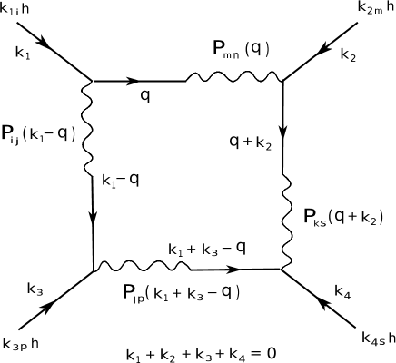
Figure 11: A one-loop Feynman diagram that appears to correct $A$, but which in fact vanishes in the limit of zero external wavevectors.

Similarly, there are one-loop diagrams that appear to correct $B$, but actually yield irrelevant contributions in the limit of zero external wavevector. A representative of such diagrams is shown in Fig. 12. It contributes to the Hamiltonian a term

$$(\delta H)_{12} \propto{\sum_{\mathbf{q}_{1},\mathbf{q}_{2},\mathbf{q}_{3}}\delta^{K}_{\mathbf{q}_{1}+\mathbf{q}_{2}+\mathbf{q}_{3}}}q_{1m}q_{2n}|\mathbf{q}_{3}|^{2}P_{ij}(\mathbf{q}_{3})h(\mathbf{q}_{1})h(\mathbf{q}_{2})h(\mathbf{q}_{3})$$

$$\times\int d^{D}qP_{ms}({\bf q}+{\bf q}_{1}+{\bf q}_{3})P_{ns}({\bf q}+{\bf q}_{2})q_{s}q_{p}({\bf q}+{\bf q}_{2})_{j}({\bf q}+{\bf q}_{1}+{\bf q}_{3})_{i}\langle|h({\bf q}+{\bf q}_{1}+{\bf q}_{3})|^{2}\rangle\langle|h({\bf q}+{\bf q}_{2})|^{2}\rangle\langle|h({\bf q}|^{2}\rangle\,.$$

Once again, as the external momenta go to zero, the $P_{ns}$ projection operator kills the $q_{s}$, and this graph vanishes.

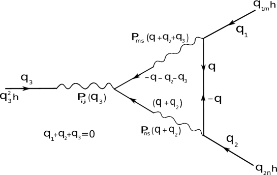
Figure 12: A typical one-loop diagram that corrects $B$ that vanishes in the limit of zero external wavevectors.

Appendix VI: Orientational correlation length $\xi$ in lowest order perturbation theory for $\kappa$

We now show that the upper and lower limits $\chi_{U}$ and $\chi_{L}$ on the asymmetry parameter $\chi$ can be extracted from the one-loop bare perturbation theory for $\kappa$, based on the diagrams (5). This calculation is the same as the RG calculation of Appendix blah, except that now we extend the integrals over wavevector down to an infrared cutoff $q_{\rm min}\equiv{2\pi\over L}$, where $L$ is the length scale on which we wish to know the effective value $\kappa_{e}$ of the bend modulus $\kappa$. Evaluating the leading order (i.e., one loop) perturbative corrections to $\kappa$ coming from wavevectors $q<{2\pi/L}$. We thereby obtain in $D=2$

$$\kappa_{e}-\kappa_{0}\approx\frac{3}{8}\left(\frac{A}{\kappa_{0}}-\frac{5B^{2}}{4\kappa_{0}^{2}}\right)\int_{2\pi/L}^{\Lambda}\frac{d^{2}q}{(2\pi)^{2}q^{4}}.$$ (V.19)

We are only interested here in the regime of parameter space in which $\kappa_{0}>0$ (indeed, that is the only regime in which this perturbative calculation even makes sense). In this regime, if the factor in parentheses above is $>0$, $\kappa_{e}>\kappa_{0}>0$, so the orientational correlation length $\xi$ (which, we recall, is the length scale on which $\kappa_{e}$ vanishes) is infinite. Hence, for $\xi$ to be finite, we must have

$$\frac{A}{\kappa_{0}}-\frac{5B^{2}}{4\kappa_{0}^{2}}>0\,,$$ (V.20)

or, equivalently,

$$B^{2}>{4A\kappa_{0}\over 5}\,.$$ (V.21)

Using our expressions (II.5) for $\kappa_{0}$, (II.22) for $B$, and (II.21) for $A$ in this inequality, we can rewrite it as an inequality for the asymmetry parameter $\chi$:

$$\chi^{2}>\chi_{{}_{{}_{L}}}^{2}=\frac{A\kappa_{0}(2\mu+\lambda)^{2}}{A(2\mu+\lambda)+5\mu^{2}}=\frac{\kappa_{0}(2\mu+\lambda)}{1+\frac{5\mu}{4(\mu+\lambda)}}=\frac{\chi_{U}^{2}}{1+\frac{5\mu}{4(\mu+\lambda)}}\,.$$ (V.22)

Note that this has exactly the same form as our expression equation (III.50) for $\chi_{L}^{2}$ obtained from the RG, with the dimensionless ${\cal O}(1)$ constant $\rho$ given by $\rho=5/4$.

Appendix VII: Vanishing of $\kappa$ on the unstable side of the separatrix

We use the flow equation (II.34) for $\kappa$ and the definition (II.38) of $g_{2}$, and note that deep inside the crumpled phase, $g_{2}\gg g_{1}$. This allows us to write

$$\frac{d\kappa}{dl}\approx\kappa(-\eta-\frac{\mathfrak{G}B^{2}}{\kappa^{3}})\,,$$ (V.23)

where $\mathfrak{G}\equiv B^{2}K_{D}k_{B}T\Lambda^{-\epsilon}$ is a constant under renormalization. Further, the choice $\epsilon=3\eta+2g_{1}$ makes the rhs of (II.36) vanish. With this choice and noting that $g_{2}>>\eta$, (V.23) becomes

$$\frac{d\kappa}{dl}=-\frac{\mathfrak{G}B^{2}}{\kappa^{2}}\,,$$ (V.24)

with $B$ now also constant under renormalization. This yields

$$\kappa^{3}(\ell)=\kappa^{3}(\ell=0)-\mathfrak{G}B^{2}\ell,$$ (V.25)

indicating that $\kappa$ vanishes and become negative in a finite renormalization group time. As one approaches the separatrix from the crumpled phase, the RG “time” required for $\kappa$ to vanish is becomes ever larger, ultimately diverging on the separatrix.

Appendix VIII: Demonstration that the hole in the middle for $T=0$ is negligibly small

In this appendix, we show that the radius $r_{0}$ of the hole in the middle of the spiral at $T=0$ is a negligible fraction of the total radius $R_{T}$ of the membrane. We consider a rectangular membrane of dimensions $L_{\parallel}\times L_{\perp}$, with $L_{\parallel}>L_{\perp}$. As discussed in the main text, for this geometry the membrane will bend along the $L_{\perp}$ direction. In our expression (I.1) for the spiral of Archimedes, we have chosen $\theta=0$ to be the innermost edge of the membrane. Hence $r_{0}$ is the size of the hole left in the center of the spiral. We can determine $r_{0}$ by minimizing the energy, which is given by

$$E=L_{||}\int_{0}^{L_{\bot}}ds\left[-{C\over R(s)}+{\kappa_{0}\over{2R^{2}(s)}}\right],$$ (V.26)

where $R(s)$ is the radius of curvature of the membrane at distance $s$ along from the inner edge of the spiral. This implies

$${ds\over d\theta}=\sqrt{r^{2}+\left({dr\over d\theta}\right)^{2}}\approx r\,,$$ (V.27)

where the approximate equality holds if ${dr\over d\theta}\ll r$. For the spiral of Archimedes (I.1), this will clearly always be true provided that $r_{0}\gg a$, since then $r(\theta)\gg a$ for all $\theta$. If $r_{0}$ is not much greater than $a$, then for a very large membrane it is clearly negligibly small compared to the total radius $R_{T}$, since the latter must diverge as $L_{\perp}\to\infty$. Thus to complete our proof that $r_{0}$ is always negligible compared to $R_{T}$, we need only consider the case $r_{0}\gg a$.

It is also clear that in this limit

$$R\approx r\,.$$ (V.28)

Both equations (V.27) and (V.28) follow from the fact that, for large $r$, the spiral is very nearly locally a circle of radius $r$. Using (V.27), we have

$$ds=rd\theta.$$ (V.29)

Differentiating (I.1) w.r.t $\theta$ gives us

$$dr={a\over 2\pi}d\theta.$$ (V.30)

Combining this along with (V.28) and (V.27) in (V.26), we obtain

$$E \approx L_{||}\int^{r_{\rm max}}_{r_{0}}dr\left[{2\pi r\over a}\left(-{C\over r}+{\kappa_{0}\over 2r^{2}}\right)\right]$$ (V.31)

$$= {2\pi L_{||}\over a}\left[-C(r_{max}-r_{0})+{\kappa_{0}\over 2}\ln({r_{max}\over r_{0}})\right],$$

where $r_{max}$ is the radius at which the spiral joins the straight segment connecting it to the other spirals. which means that each spiral has a total length of $({L_{\bot}\over 2}-{r_{\rm max}\over 2})$ available to coil up into a spiral. We can calculate $r_{\rm max}$ by first taking the ratio of (V.29) and (V.30); this gives

$${ds\over dr}={2\pi r\over a}.$$ (V.32)

Integrating the above equation over one of the two spirals yields

$${L_{\bot}-r_{\rm max}\over 2}=\pi{(r_{\rm max}^{2}-r_{0}^{2})\over a}.$$ (V.33)

Assuming $r_{\rm max}>>a$ (which can be verified a posteriori), so that ${r_{\rm max}^{2}\over a}>>r_{\rm max}$, we obtain from Eq. (V.33),

$$r_{\rm max}=\sqrt{{aL_{\bot}\over 2\pi}+r_{0}^{2}}.$$ (V.34)

Now assuming that $r_{0}<<\sqrt{aL_{\bot}}$, (which will also be verified a posteriori), Eq. (V.34) can be approximated as

$$r_{\rm max}\approx\sqrt{{aL_{\bot}\over 2\pi}}+\sqrt{{\pi r_{0}^{2}\over 2aL_{\bot}}}r_{0}.$$ (V.35)

The second term on the right hand side of Eq. (V.35) is negligible compared to $r_{0}$, provided our assumption of $r_{0}<<\sqrt{aL_{\bot}}$ is correct, and hence can be neglected, in eq. (V.31) for the energy, relative to the $r_{0}$ terms in $(r_{\rm max}-r_{0})$. Thus Eq. (V.31) can be approximated as

$$E={2\pi L_{||}\over a}\left[-C\sqrt{{aL_{\bot}\over 2\pi}}+C_{0}r_{0}+{\kappa_{0}\over 2}\ln\left(\sqrt{aL_{\bot}\over 2\pi r_{0}^{2}}\right)\right].$$

(V.36)

Minimizing this expression for the energy over $r_{0}$ gives us

$$r_{0}={\kappa_{0}\over 2C}.$$ (V.37)

We note that since this is independent of $L_{\bot}$, $r_{0}$ will always be $<<\sqrt{aL_{\bot}}$ (as assumed above) if $L_{\bot}>>{\kappa_{0}^{2}\over C^{2}a}$. Also since (V.35) gives $r_{\rm max}\approx\sqrt{{aL_{\bot}\over 2\pi}}$, we see that the a posteriori assumption $r_{\rm max}>>a$ will always be satisfied provided $L_{\bot}>>a$, which it must be for us to describe our system as a membrane. Thus all our assumptions are well-validated. Notice Eq. (V.37) together with Eq. (II.5) yields that $r_{0}$ can be tuned to zero by tuning $\chi$.

We lastly comment on the expansion of $r_{0}$ due to thermal fluctuations. Since $L_{H}(s)$ has a monotonic dependence on $d(s)\propto s^{1/3}$, for the innermost turns of the spiral near its core, we note that $L_{H}$ is very small. This means $L_{H}\ll\xi_{NL}$ for the first few layers, and hence the nonlinear fluctuation-corrections to $\kappa_{0}$ are small. Thus even at finite $T$, the effective bend modulus for the first few turns of the spiral is same as $\kappa_{0}$, and $r_{0}$ is still given by (V.37). This also means the shape of the spiral near its core is given by Eq. (III.30) with $\eta=0$ and $\nu=1$. Thus the form of the spiral near its core in the stable spiral phase with $\chi^{2}<\chi_{L}^{2}$ is different from its shape near the outermost turns.

References

- Nelson et al. (2004) D. R. Nelson, T. Piran, and S. Weinberg, Statistical mechanics of membranes and surfaces (World Scientific, 2004).
- Cates (1984) M. E. Cates, “Statics and dynamics of polymeric fractals,” Phys. Rev. Lett. 53, 926–929 (1984).
- Cates (1985) M. E. Cates, “The fractal dimension and connectivity of random surfaces,” Phys. Lett. B 161, 363–367 (1985).
- Kantor et al. (1987) Y. Kantor, M. Kardar, and D. R. Nelson, “Tethered surfaces: Statics and dynamics,” Phys. Rev. A 35, 3056 (1987).
- Paczuski et al. (1988) M. Paczuski, M. Kardar, and D. R. Nelson, “Landau theory of the crumpling transition,” Phys. Rev. Lett. 60, 2638–2640 (1988).
- Mermin and Wagner (1966) N. D. Mermin and H. Wagner, “Absence of ferromagnetism or antiferromagnetism in one-or two-dimensional isotropic heisenberg models,” Phys. Rev. Lett. 17, 1133 (1966).
- Hohenberg (1967) P. C. Hohenberg, “Existence of long-range order in one and two dimensions,” Phys. Rev. 158, 383 (1967).
- Guitter et al. (1989) E. Guitter, F. David, S. Leibler, and L. Peliti, “Thermodynamical behavior of polymerized membranes,” J. Physique 50, 1787–1819 (1989).
- David and Wiese (1996) F. David and K. J. Wiese, “Scaling of self-avoiding tethered membranes: 2-loop renormalization group results,” Phys. Rev. Lett. 76, 4564 (1996).
- Wiese and David (1997) K. J. Wiese and F. David, “New renormalization group results for scaling of self-avoiding tethered membranes,” Nucl. Phys. B 487, 529–632 (1997).
- Domb (2000) C. Domb, Phase transitions and critical phenomena, Vol. 19 (Academic press, 2000).
- López-Montero et al. (2012) I. López-Montero, R. Rodríguez-García, and F. Monroy, “Artificial spectrin shells reconstituted on giant vesicles,” J. Phys. Chem. Lett. 3, 1583–1588 (2012).
- Archimedes (-225) Archimedes, On Spirals (Syracuse University Press, Syracuse (Sicily), -225).
- Note (1) Unsurprisingly, inversion-symmetric tethered membranes are always uncrumpled and flat at temperature .
- Helfrich (1978) W. Helfrich, “Steric interaction of fluid membranes in multilayer systems,” Z. Naturforsch. A 33, 305–315 (1978).
- Doussal and Radzihovsky (1992) P. Le Doussal and L. Radzihovsky, “Self-consistent theory of polymerized membranes,” Phys. Rev. Lett. 69, 1209 (1992).
- Lee et al. (2008) C. Lee, X. Wei, J. W. Kysar, and J. Hone, “Measurement of the elastic properties and intrinsic strength of monolayer graphene,” Science 321, 385 (2008).
- Jussila et al. (2016) H. Jussila, H. Yang, N. Granqvist, and Z. Sun, “Surface plasmon resonance for characterization of large-area atomic-layer graphene film,” Optica 3, 151 (2016).
- Peliti and Leibler (1985) L. Peliti and S. Leibler, “Effects of thermal fluctuations on systems with small surface tension,” Phys. Rev. Lett. 54, 1690 (1985).
- Chaikin and Lubensky (2000) P. M. Chaikin and T. C. Lubensky, Principles of condensed matter physics (Cambridge university press, 2000).
- Aronovitz and Lubensky (1988) J. A. Aronovitz and T. C. Lubensky, “Fluctuations of solid membranes,” Phys. Rev. Lett. 60, 2634 (1988).
- Leibler (1986) S. Leibler, “Curvature instability in membranes,” J. Physique 47, 507–516 (1986).
- Note (2) In we have ignored a nonlinear term of the form that would originate from the expansion of the area element in Monge gauge, for small fluctuations. This has the critical dimension of and hence is formally as relevant as the - and -terms are. This will generate additional corrections to , and at or higher, in addition to generating a correction to itself (which is ). Nonetheless, the stable fixed point structure of , and still holds and all our results should work. In any case, the RG eigenvalue of as the coefficient of the nonlinear term is , where as as the coefficient of the corresponding linear term has its RG eigenvalue . Noting that , near , as the coefficient of the linear term dominates over the corresponding nonlinear term for large length scales. Hence, this nonlinear term may be ignored.
- Note (3) This expression for is not exact, but is valid in the limit of nearly flat membrane, for which .
- Wilson (1975) K. G. Wilson, “The renormalization group: Critical phenomena and the kondo problem,” Rev. Mod. Phys. 47, 773 (1975).
- Note (4) The alert and well-informed reader will notice that both the position of this fixed point, and the value of that keeps fixed, are slightly different from those obtained by Aronovitz and Lubensky (1988). This difference is simply due to the fact that we have analytically continued our model to dimensions D2 in a slightly different way than they did Aronovitz and Lubensky (1988); our results should reduce to theirs in D=2, where the ambiguity of continuation in dimension disappears.
- Toner (1990) J. Toner, “New phase of matter in lamellar phases of tethered, crystalline membranes,” Phys. Rev. Lett. 64, 1741 (1990).
- Landau and Lifshitz (1970) L. D. Landau and E. M. Lifshitz, Theory of elasticity (Pergamon Press, 1970).
- Kaes et al. (1990) J. Kaes, H. P. Duwe, and E. Sackmann, “Bending elastic moduli of lipid bilayers: modulation by solutes,” J. Phys. France 51, 945 (1990).
- Kamal et al. (2009) M. M. Kamal, D. Mills, M. Grzybek, and J. Howard, “Measurement of the membrane curvature preference of phospholipids reveals only weak coupling between lipid shape and leaflet curvature,” Proc. Nat. Acad. Sc. (USA) 106, 22245––22250 (2009).

References

- Nelson et al. (2004) D. R. Nelson, T. Piran, and S. Weinberg, Statistical mechanics of membranes and surfaces (World Scientific, 2004).
- Cates (1984) M. E. Cates, “Statics and dynamics of polymeric fractals,” Phys. Rev. Lett. 53, 926–929 (1984).
- Cates (1985) M. E. Cates, “The fractal dimension and connectivity of random surfaces,” Phys. Lett. B 161, 363–367 (1985).
- Kantor et al. (1987) Y. Kantor, M. Kardar, and D. R. Nelson, “Tethered surfaces: Statics and dynamics,” Phys. Rev. A 35, 3056 (1987).
- Paczuski et al. (1988) M. Paczuski, M. Kardar, and D. R. Nelson, “Landau theory of the crumpling transition,” Phys. Rev. Lett. 60, 2638–2640 (1988).
- Mermin and Wagner (1966) N. D. Mermin and H. Wagner, “Absence of ferromagnetism or antiferromagnetism in one-or two-dimensional isotropic heisenberg models,” Phys. Rev. Lett. 17, 1133 (1966).
- Hohenberg (1967) P. C. Hohenberg, “Existence of long-range order in one and two dimensions,” Phys. Rev. 158, 383 (1967).
- Guitter et al. (1989) E. Guitter, F. David, S. Leibler, and L. Peliti, “Thermodynamical behavior of polymerized membranes,” J. Physique 50, 1787–1819 (1989).
- David and Wiese (1996) F. David and K. J. Wiese, “Scaling of self-avoiding tethered membranes: 2-loop renormalization group results,” Phys. Rev. Lett. 76, 4564 (1996).
- Wiese and David (1997) K. J. Wiese and F. David, “New renormalization group results for scaling of self-avoiding tethered membranes,” Nucl. Phys. B 487, 529–632 (1997).
- Domb (2000) C. Domb, Phase transitions and critical phenomena, Vol. 19 (Academic press, 2000).
- López-Montero et al. (2012) I. López-Montero, R. Rodríguez-García, and F. Monroy, “Artificial spectrin shells reconstituted on giant vesicles,” J. Phys. Chem. Lett. 3, 1583–1588 (2012).
- Archimedes (-225) Archimedes, On Spirals (Syracuse University Press, Syracuse (Sicily), -225).
- Note (1) Unsurprisingly, inversion-symmetric tethered membranes are always uncrumpled and flat at temperature .
- Helfrich (1978) W. Helfrich, “Steric interaction of fluid membranes in multilayer systems,” Z. Naturforsch. A 33, 305–315 (1978).
- Doussal and Radzihovsky (1992) P. Le Doussal and L. Radzihovsky, “Self-consistent theory of polymerized membranes,” Phys. Rev. Lett. 69, 1209 (1992).
- Lee et al. (2008) C. Lee, X. Wei, J. W. Kysar, and J. Hone, “Measurement of the elastic properties and intrinsic strength of monolayer graphene,” Science 321, 385 (2008).
- Jussila et al. (2016) H. Jussila, H. Yang, N. Granqvist, and Z. Sun, “Surface plasmon resonance for characterization of large-area atomic-layer graphene film,” Optica 3, 151 (2016).
- Peliti and Leibler (1985) L. Peliti and S. Leibler, “Effects of thermal fluctuations on systems with small surface tension,” Phys. Rev. Lett. 54, 1690 (1985).
- Chaikin and Lubensky (2000) P. M. Chaikin and T. C. Lubensky, Principles of condensed matter physics (Cambridge university press, 2000).
- Aronovitz and Lubensky (1988) J. A. Aronovitz and T. C. Lubensky, “Fluctuations of solid membranes,” Phys. Rev. Lett. 60, 2634 (1988).
- Leibler (1986) S. Leibler, “Curvature instability in membranes,” J. Physique 47, 507–516 (1986).
- Note (2) In we have ignored a nonlinear term of the form that would originate from the expansion of the area element in Monge gauge, for small fluctuations. This has the critical dimension of and hence is formally as relevant as the - and -terms are. This will generate additional corrections to , and at or higher, in addition to generating a correction to itself (which is ). Nonetheless, the stable fixed point structure of , and still holds and all our results should work. In any case, the RG eigenvalue of as the coefficient of the nonlinear term is , where as as the coefficient of the corresponding linear term has its RG eigenvalue . Noting that , near , as the coefficient of the linear term dominates over the corresponding nonlinear term for large length scales. Hence, this nonlinear term may be ignored.
- Note (3) This expression for is not exact, but is valid in the limit of nearly flat membrane, for which .
- Wilson (1975) K. G. Wilson, “The renormalization group: Critical phenomena and the kondo problem,” Rev. Mod. Phys. 47, 773 (1975).
- Note (4) The alert and well-informed reader will notice that both the position of this fixed point, and the value of that keeps fixed, are slightly different from those obtained by Aronovitz and Lubensky (1988). This difference is simply due to the fact that we have analytically continued our model to dimensions D2 in a slightly different way than they did Aronovitz and Lubensky (1988); our results should reduce to theirs in D=2, where the ambiguity of continuation in dimension disappears.
- Toner (1990) J. Toner, “New phase of matter in lamellar phases of tethered, crystalline membranes,” Phys. Rev. Lett. 64, 1741 (1990).
- Landau and Lifshitz (1970) L. D. Landau and E. M. Lifshitz, Theory of elasticity (Pergamon Press, 1970).
- Kaes et al. (1990) J. Kaes, H. P. Duwe, and E. Sackmann, “Bending elastic moduli of lipid bilayers: modulation by solutes,” J. Phys. France 51, 945 (1990).
- Kamal et al. (2009) M. M. Kamal, D. Mills, M. Grzybek, and J. Howard, “Measurement of the membrane curvature preference of phospholipids reveals only weak coupling between lipid shape and leaflet curvature,” Proc. Nat. Acad. Sc. (USA) 106, 22245––22250 (2009).