Role of $\sigma R^{2}+\gamma R_{\mu\nu}T^{\mu\nu}$ Model on Anisotropic Polytropes

Abstract

This paper analyzes the anisotropic stellar evolution governed by polytropic equation of state in the framework of $f(R,T,Q)$ gravity, where $Q=R_{ab}T^{ab}$. We construct the field equations, hydrostatic equilibrium equation and trace equation to obtain their solutions numerically under the influence of $\sigma R^{2}+\gamma Q$ gravity model, where $\sigma$ and $\gamma$ are arbitrary constants. We examine the dependence of various physical characteristics such as radial/tangential pressure, energy density, anisotropic factor, total mass and surface redshift for specific values of the model parameters. The physical acceptability of the considered model is discussed by verifying the validity of energy conditions, causality condition and adiabatic index. We also study the effects arising due to strong non-minimal matter-curvature coupling on anisotropic polytropes. It is found that the polytropic stars are stable and their maximum mass point lies within the required observational Chandrasekhar limit.

Keywords: $f(R,T,Q)$ gravity; Compact objects; Polytropic equation of state.
PACS: 04.50.Kd; 04.40.Dg.

1 Introduction

The fascinating phenomenon of gravitational collapse and its final state have played an inspiring role for researchers in astrophysics as well as modern cosmology. This process is responsible to produce remnants of massive stars known as compact objects. In the transformation of stars, a stage appears when the radiation pressure directed outward no longer counter balances the inward directed gravitational pull and they undergo stellar death. The final outcome of collapse completely depends upon the original mass of the star. Similar to other ordinary stars, compact stars are very common and their formation lead to white dwarfs, neutron stars and black holes. There are many evidences for the formation of white dwarfs and neutron stars while for black holes, the first evidence is provided by the astronomers in Andromeda galaxy and later in M104, NGC3115, M106 and Milky Way galaxies [1].

An astronomical object comprising polytropic equation of state (EoS) is referred as polytropic star or polytropes. The polytropic EoS provides an excellent advancement for adiabatic systems. In the interior of compact objects, pressure produced from the degeneracy of electrons and neutrons exists which is used to overcome the effects of gravity. Tooper [2], as a pioneer, inspected the structure of relativistic objects by considering polytropic EoS for perfect fluid distribution. Thirukkanesh and Ragel [3] investigated two cases of polytropic EoS with polytropic exponents $2$ and $\frac{3}{2}$ to describe the properties of anisotropic compact objects for static spherically symmetric spacetime. Herrera et al. [4] examined the conformally flat polytropic stars satisfying anisotropic spherically symmetric fluid distribution. They showed physical properties of these polytropes graphically for different values of polytropic index. Ngubelanga and Maharaj [5] studied Einstein-Maxwell system of equations with anisotropy using polytropic EoS and generated exact solutions for different polytropic indices. Sharif and Sadiq [6] extended the work of [4] for static cylindrical system and also examined the effects of charge on anisotropic conformally flat polytropes in spherical symmetry.

The surface gravitational redshift $(z_{s})$ is an interesting phenomenon in which electromagnetic radiation are redshifted in frequency in a region of strong gravitational potential. This provides the physics of strong relation between particles in the interior geometry of star and its EoS. For static spherical configurations, maximum limit for the surface redshift corresponding to isotropic as well as anisotropic fluid are obtained as $z_{s}\leq 2$ [7] and $z_{s}\leq 5.211$ [8], respectively. Böhmer and Harko [9] derived the upper and lower limits for few physical parameters corresponding to anisotropic fluid with cosmological constant. They also studied the total energy bounds and $z_{s}$ in terms of anisotropic factor.

In the age of current cosmic accelerated expansion, alternative theories to general relativity (GR) have played a vital role to discover hidden mysteries of dark energy and dark matter. The $f(R)$ gravity [10] is the simplest extension of GR constructed by taking an arbitrary function $f(R)$ instead of Ricci scalar $R$ in the Einstein-Hilbert action. Harko et al. [11] proposed $f(R,T)$ gravity, where $T$ denotes trace of the energy-momentum tensor. The matter-curvature coupling yields a source term which may provide interesting results. It can produce a matter dependent deviation from geodesic motion and also describe dark energy, dark matter interactions as well as late-time acceleration. Motivated by this argument, Haghani et al. [12] formulated a more extended theory called $f(R,T,Q)$ gravity which involves a strong non-minimal coupling of matter and geometry.

Odintsov and Sáez-Gómes [13] analyzed various cosmological solutions and reconstructed the corresponding gravitational action of $f(R,T,Q)$ gravity. Sharif and Zubair examined the validity of energy conditions [14] and thermodynamical laws [15] in this theory. Ayuso et al. [16] checked the consistency and stability of this theory for different functional forms. The physical characteristics of some particular compact stars for different distributions of matter are also investigated [17]. Baffou et al. [18] inspected the stability of two different models of this gravity using the de Sitter and power-law solutions. Yousaf et al. [19] explored stability of anisotropic dissipative cylindrical system as well as non-static anisotropic stellar models. The stability of Einstein universe using inhomogeneous perturbations is also discussed in the same theory [20]. Recently, we have studied non-static dust spherical solution and analyzed the mass-radius relation as well as redshift parameter corresponding to radial and temporal coordinates [21].

The study of physical properties and stability of polytropic stars is of fundamental importance in modified gravitational theories. Henttunen et al. [22] examined the stellar configurations in $f(R)$ theory by considering different cases of polytropic EoS. They derived the solution analytically near the center of the star and discussed the possibility of constructing $f(R)$ theory consistent with the solar system experiments. Orellana et al. [23] investigated the mass-radius relation as well as density profiles using realistic polytropic EoS in $f(R)$ gravity. Henttunen and Vilja [24] observed the consistency of $f(R)$ gravity models on polytropes for static spherical configuration. The stellar equilibrium configuration of quark as well as polytropic stars are studied in $f(R,T)$ gravity [25]. Sharif and Siddiqa [26] analyzed the stellar structure of compact stars comprising MIT bag model and polytropic EoS in $f(R,T)$ gravity. They also obtained the effects of charge on static spherically symmetric polytropes for isotropic fluid distribution [27].

From astrophysical observations, the scenario of stellar system analyzes how stellar solution satisfies some general physical features of compact objects. This paper is therefore devoted to explore physical characteristics as well as stability of anisotropic polytropes to evaluate the constraints for which the system of stellar equations is physically realistic in $f(R,T,Q)$ gravity. The pattern of this paper is as follows. The next section provides basic formalism of $f(R,T,Q)$ gravity while in section 3, we derive equations for static spherically symmetric spacetime corresponding to anisotropic fluid. In section 4, we construct a system of differential equations for two cases of polytropic EoS and study physical features as well as stability of compact stars graphically. We summarize the whole discussion in the last section.

2 Formalism of $f(R,T,Q)$ Gravity

The basic formulation of $f(R,T,Q)$ gravity is established on the strong association of non-minimal coupling of geometry and matter. The action of this modified gravity in the presence of matter Lagrangian $\mathcal{L}_{m}$ is defined as [12]

$$A=\frac{1}{2\kappa^{2}}\int\sqrt{-g}\left({f(R,T,Q)+\mathcal{L}_{m}}\right)d^{4}x,$$ (1)

where $\kappa^{2}(=1)$ is the coupling constant and $g$ is the determinant of the metric tensor $(g_{ab})$. The standard energy-momentum tensor whose matter action depends only on $g_{ab}$ and not on its derivative is given by [28]

$$T_{ab}=-\frac{2}{\sqrt{-g}}\frac{\delta(\sqrt{-g}\mathcal{L}_{m})}{\delta g^{ab}}=g_{ab}\mathcal{L}_{m}-\frac{2\partial\mathcal{L}_{m}}{\partial g^{ab}}.$$ (2)

The corresponding field equations are

$$G_{ab} = \frac{1}{f_{R}-f_{Q}\mathcal{L}_{m}}\left[(1+f_{T}+\frac{1}{2}Rf_{Q})T_{ab}+\left\{\frac{1}{2}(f-Rf_{R})-\mathcal{L}_{m}f_{T}\right.\right.$$ (3)

$$- \left.\left.\frac{1}{2}\nabla_{\alpha}\nabla_{\beta}(f_{Q}T^{\alpha\beta})\right\}g_{ab}-(g_{ab}\Box-\nabla_{a}\nabla_{b})f_{R}+\nabla_{\alpha}\nabla_{(a}[T_{b)}^{\alpha}f_{Q}]\right.$$

$$- \left.\frac{1}{2}\Box(f_{Q}T_{ab})-2f_{Q}R_{\alpha(a}T_{b)}^{\alpha}+2(f_{T}g^{\alpha\beta}+f_{Q}R^{\alpha\beta})\frac{\partial^{2}\mathcal{L}_{m}}{\partial g^{ab}\partial g^{\alpha\beta}}\right],$$

where $f_{R}\equiv\frac{\partial f}{\partial R}$, $f_{T}\equiv\frac{\partial f}{\partial T}$ and $\Box\equiv\nabla^{a}\nabla_{a}$. Notice that for $Q=0$, one can retrieve the field equations of $f(R,T)$ gravity which can further be reduced to $f(R)$ gravity for $T=0$ and consequently, the results of GR are obtained for $f(R)=R$. The covariant divergence of the field equations (3) leads to

$$\nabla^{a}T_{ab} = \frac{2}{2(1+f_{T})+Rf_{Q}}\Big{[}\nabla_{a}\left(f_{Q}R^{a\mu}T_{\mu b}\right)+\nabla_{b}(\mathcal{L}_{m}f_{T})-G_{ab}\nabla^{a}(f_{Q}\mathcal{L}_{m})\Big{.}$$ (4)

$$- \Big{.}\frac{1}{2}(f_{Q}R_{\alpha\beta}+f_{T}g_{\alpha\beta})\nabla_{b}T^{\alpha\beta}-\frac{1}{2}[\nabla^{a}(Rf_{Q})+2\nabla^{a}f_{T}]T_{ab}\Big{]}.$$

It is mentioned here that standard conservation law does not hold in this modified theory similar to other modified theories having non-minimal coupling of matter and geometry [11]. The trace of the field equations (3) is calculated in the following form

$$-R = \frac{1}{f_{R}-f_{Q}\mathcal{L}_{m}}\left[(1+\frac{1}{2}Rf_{Q})T+2(f-Rf_{R})-\nabla_{\alpha}\nabla_{\beta}(f_{Q}T^{\alpha\beta})\right.$$ (5)

$$- \left.3\Box f_{R}-\frac{1}{2}\Box(Tf_{Q})-2f_{Q}R_{\alpha\beta}T^{\alpha\beta}\right],$$

In compact objects, pressure anisotropy is an important matter ingredient which affects their evolution. It is well-known that stellar models are mostly rotating and anisotropic in nature. The anisotropic factor plays a vital role in different dynamical phases of stellar evolution [29]. The influence of anisotropy arises when the radial component of pressure differs from the tangential or angular component. The standard form of the energy-momentum tensor capable of supporting anisotropic matter distribution is

$$T_{ab}=(\rho+p_{t})U_{a}U_{b}+(p_{r}-p_{t})V_{a}V_{b}-p_{t}g_{ab},$$ (6)

where $\rho$, $p_{t}$ and $p_{r}$ represent the energy density, tangential pressure and radial pressure of the fluid, respectively. In comoving coordinates, $U_{a}=\sqrt{g_{00}}(1,0,0,0)$ denotes four velocity which satisfies the condition $U_{a}U^{a}=1$ whereas $V_{a}$ expresses the radial four-vector satisfying $V_{a}V^{a}=-1$. For anisotropic fluid distribution, we have $\mathcal{L}_{m}=\rho$ that leads to $\frac{\partial^{2}\mathcal{L}_{m}}{\partial g^{ab}\partial g^{\mu\nu}}=0$ [12].

In order to discuss physical characteristics of anisotropic polytropes, we consider a particular functional form $f(R,T,Q)=\sigma R^{m}+\gamma Q^{n}$, where $m$ and $n$ are constants. To deal with this theory free from Ostrogradski instabilities, we take $m\neq 1$. However, this model generates stable theory for $n=1$ exhibiting a strong coupling between its arguments by providing Einstein-Hilbert term involving canonical scalar field with non-minimal variation coupling of the energy-momentum and Ricci tensors. This functional form could support to unveil many mysterious as well as unexplored fascinating issues of the universe. This particular model along with $m=2$, $n=1$ and constant $\gamma$ helps to study various cosmological issues. Haghani et al. [12] examined some cosmological aspects with $n=1$. Yousaf et al. [19] discussed this model with $m=2$, $n=1$ and analyzed stable structure of compact objects for anisotropic spherical distribution by taking $\gamma>0$. Astashenok et al. [30] found that for the model $R+\sigma R^{2}$ of $f(R)$ gravity, $\sigma>0$ yields better results to examine the physical properties of compact stars. The case $\sigma=0$ in $\sigma R^{m}+\gamma Q^{n}$ model gives matter-curvature gravitational interaction only through coupling between the Ricci and energy-momentum tensors. Such modeling could smoothly describe dynamical implication on interesting issues of cosmos different from $f(R,T)$ gravity.

Here, we take $m=2,~{}n=1,~{}\sigma>0$ and $\gamma>0$. Substituting $f(R,T,Q)=\sigma R^{2}+\gamma Q$ model along with $\mathcal{L}_{m}=\rho$ in Eq.(3), it follows that

$$G_{ab} = \frac{1}{2\sigma R-\gamma\rho}\left[T_{ab}+\frac{\gamma}{2}RT_{ab}-\frac{1}{2}(\sigma R^{2}-\gamma Q)g_{ab}-\frac{\gamma}{2}\nabla_{\alpha}\nabla_{\beta}(T^{\alpha\beta})g_{ab}\right.$$ (7)

$$- \left.2\sigma g_{ab}\Box R+2\sigma\nabla_{\alpha}\nabla_{\beta}(R)+\gamma\nabla_{\alpha}\nabla_{(a}T_{b)}^{a}-\frac{\gamma}{2}\Box T_{ab}-2\gamma R_{\alpha(a}T_{b)}^{\alpha}\right],$$

for which $G_{ab}$ is the usual Einstein tensor. Also, for the considered model, the non-conservation equation of the energy-momentum tensor yields

$$\nabla^{a}T_{ab} = \frac{2\gamma}{2+\gamma R}\left[\nabla_{a}(R^{a\mu}T_{\mu b})-G_{ab}\nabla^{a}(\rho)-\frac{1}{2}(R_{\alpha\beta})\nabla_{b}T^{\alpha\beta}-\frac{1}{2}\nabla^{a}(R)T_{ab}\right].$$

and the trace equation (5) turns out to be

$$-R = \frac{1}{2\sigma R-\gamma\rho}\left[T+\frac{\gamma}{2}RT-2\sigma R^{2}-\gamma\nabla_{\alpha}\nabla_{\beta}(T^{\alpha\beta})-6\sigma\Box(R)-\frac{\gamma}{2}\Box(T)\right].$$

3 System of Equations

To describe the interior geometry of a star, we take static spherically symmetric configuration

$$ds^{2}_{-}=e^{\mu(r)}dt^{2}-e^{\lambda(r)}dr^{2}-r^{2}(d\theta^{2}+\sin^{2}\theta d\phi^{2}).$$ (10)

For the corresponding line element, the field equations (7) along with anisotropic matter content (6) yield

$$e^{-\lambda}(\frac{\lambda^{\prime}}{r}-\frac{1}{r^{2}})+\frac{1}{r^{2}} = \frac{1}{2\sigma R-\gamma\rho}\left[\rho+\frac{\gamma}{2}R\rho-\frac{\sigma}{2}R^{2}+e^{-\lambda}\left\{\frac{\gamma}{8}\mu^{\prime 2}\rho\right.\right.$$ (11)

$$- \left.\left.\sigma R^{\prime}\left(\lambda^{\prime}-\frac{4}{r}\right)+\gamma p_{r}\left(\frac{\lambda^{\prime}}{r}-\frac{1}{r^{2}}\right)+2\sigma R^{\prime\prime}\right.\right.$$

$$- \left.\left.\frac{\gamma}{2}\rho^{\prime}\left(\frac{\lambda^{\prime}}{2}-\frac{5\mu^{\prime}}{2}-\frac{2}{r}\right)+\frac{\gamma}{2}\left(\rho^{\prime\prime}-p_{r}^{\prime\prime}\right)+\frac{\gamma}{r}p_{t}^{\prime}\right.\right.$$

$$- \left.\left.\frac{\gamma}{2}p_{r}^{\prime}\left(\frac{4}{r}-\frac{\lambda^{\prime}}{2}\right)\right\}\right],$$

$$e^{-\lambda}\left(\frac{\mu^{\prime}}{r}+\frac{1}{r^{2}}\right)-\frac{1}{r^{2}} = \frac{1}{2\sigma R-\gamma\rho}\left[p_{r}+\frac{\sigma}{2}R^{2}+\frac{\gamma}{2}Rp_{r}+e^{-\lambda}\left\{\frac{\gamma\rho}{2}\right.\right.$$ (12)

$$\times \left.\left.\left(\mu^{\prime 2}-\mu^{\prime}\lambda^{\prime}\right)+\frac{\gamma}{2}p_{r}\left(\frac{2\mu^{\prime}}{r}-\mu^{\prime\prime}+\frac{6}{r^{2}}+\lambda^{\prime\prime}\right.\right.\right.$$

$$+ \left.\left.\left.\mu^{\prime}\lambda^{\prime}+\frac{4\lambda^{\prime}}{r}+\frac{3\lambda^{\prime 2}}{2}\right)+2\gamma p_{t}\left(\frac{\lambda^{\prime}}{r}-\frac{1}{r^{2}}\right)\right.\right.$$

$$+ \left.\left.\frac{\gamma}{r}p_{t}^{\prime}-\frac{\gamma}{2}\mu^{\prime}\rho^{\prime}+\frac{\gamma}{2}p_{r}^{\prime}\left(\frac{\mu^{\prime}}{2}+\frac{2}{r}+2\lambda^{\prime}\right)\right.\right.$$

$$- \left.\left.2\sigma R^{\prime}\left(\frac{\mu^{\prime}}{2}+\frac{2}{r}\right)\right\}\right],$$

$$\frac{\mu^{\prime\prime}}{2}-\frac{\lambda^{\prime}}{2r}+\frac{\mu^{\prime}}{2r}+\frac{\mu^{\prime 2}}{4}-\frac{\mu^{\prime}\lambda^{\prime}}{4} = \frac{1}{2\sigma R-\gamma\rho}\left[e^{\lambda}\left(p_{t}+\frac{\gamma}{2}Rp_{t}+\frac{\sigma}{2}R^{2}\right)+\frac{\gamma}{4}\mu^{\prime 2}\rho\right.$$ (13)

$$- \left.\frac{\gamma}{2}p_{r}\left(\frac{\mu^{\prime}\lambda^{\prime}}{2}-\frac{\mu^{\prime 2}}{2}-\mu^{\prime\prime}+\frac{2}{r^{2}}+\frac{\lambda^{\prime}}{r}-\frac{\mu^{\prime}}{r}\right)\right.$$

$$+ \left.\gamma p_{t}\left(\frac{3}{r^{2}}-\frac{\mu^{\prime}}{2r}\right)+\frac{\gamma}{2}p_{r}^{\prime}\left(\mu^{\prime}-\frac{\lambda^{\prime}}{2}+\frac{2}{r}\right)+\frac{\gamma}{2}p_{t}^{\prime}\right.$$

$$\times \left.\left(\frac{\mu^{\prime}}{2}-\frac{\lambda^{\prime}}{2}+\frac{4}{r}\right)+2\sigma R^{\prime}\left(\frac{\lambda^{\prime}}{2}-\frac{\mu^{\prime}}{2}-\frac{1}{r}\right)\right.$$

$$+ \left.\frac{\gamma}{2}\left(p_{r}^{\prime\prime}+p_{t}^{\prime\prime}\right)-2\sigma R^{\prime\prime}\right],$$

where prime shows derivative with respect to radial coordinate. Moreover, from the non-conservation of the energy-momentum tensor (LABEL:8), the hydrostatic equilibrium equation which is also a generalized form of Tolman-Oppenheimer-Volkoff equation in $f(R,T,Q)$ gravity is derived as

$$p_{r}^{\prime}+\left(\rho+p_{r}\right)\frac{\mu^{\prime}}{2}+\frac{2}{r}\left(p_{r}-p_{t}\right) = \frac{2\gamma}{2+\gamma R}\left[p_{r}\left(\frac{3\mu^{\prime\prime}\lambda^{\prime}}{4}+\frac{\mu^{\prime}\lambda^{\prime\prime}}{4}-\frac{\mu^{\prime\prime\prime}}{2}-\frac{3\mu^{\prime}\mu^{\prime\prime}}{4}\right.\right.$$ (14)

$$+ \left.\left.\frac{\lambda^{\prime\prime}}{r}-\frac{\mu^{\prime\prime}}{r}+\frac{\lambda^{\prime}}{r^{2}}-\frac{\mu^{\prime 3}}{8}+\frac{\mu^{\prime}\lambda^{\prime}}{r}+\frac{3\mu^{\prime 2}\lambda^{\prime}}{8}\right.\right.$$

$$- \left.\left.\frac{\mu^{\prime}\lambda^{\prime 2}}{4}-\frac{\lambda^{\prime 2}}{r}\right)+\rho\left(\frac{\mu^{\prime 2}\lambda^{\prime}}{8}-\frac{\mu^{\prime}\mu^{\prime\prime}}{4}-\frac{\mu^{\prime 2}}{2r}\right.\right.$$

$$+ \left.\left.\frac{\lambda^{\prime}}{r^{2}}\right)+p_{t}\left(\frac{2}{r^{3}}-\frac{2e^{\lambda}}{r^{3}}-\frac{\lambda^{\prime}}{r^{2}}+\frac{\mu^{\prime}}{r^{2}}\right)+R\left(\rho^{\prime}\right.\right.$$

$$+ \left.\left.\frac{2}{r}(p_{r}-p_{t})\right)+\frac{p_{r}^{\prime}}{2}\left(\frac{\mu^{\prime}\lambda^{\prime}}{4}+\frac{\lambda^{\prime}}{r}-\frac{\mu^{\prime 2}}{4}-\frac{\mu^{\prime\prime}}{2}\right)\right.$$

$$- \left.\frac{\rho^{\prime}}{2}\left(\frac{\mu^{\prime\prime}}{2}+\frac{\mu^{\prime}}{r}-\frac{\mu^{\prime}\lambda^{\prime}}{4}+\frac{\mu^{\prime 2}}{4}\right)+p_{t}^{\prime}\left(\frac{1}{r^{2}}-\frac{e^{\lambda}}{r^{2}}\right.\right.$$

$$- \left.\left.\frac{\lambda^{\prime}}{2r}+\frac{\mu^{\prime}}{2r}\right)-\frac{R^{\prime}}{2}\left(\rho-p_{r}-2p_{t}\right)\right].$$

It is interesting to mention here that Eq.(14) reduces to the ideal conservation equation in GR [31, 32] for $\gamma=0$. For the proposed model, the trace equation (LABEL:9) corresponding to anisotropic distribution leads to

$$R^{\prime\prime} = \frac{e^{\lambda}}{6\sigma}\left[p_{r}+2p_{t}-\rho+\frac{\gamma}{2}R(p_{r}+2p_{t}+\rho)\right]-R^{\prime}\left(\frac{\mu^{\prime}}{2}-\frac{\lambda^{\prime}}{2}+\frac{2}{r}\right)-\frac{\gamma}{12\sigma}$$ (15)

$$\times \left(\rho^{\prime\prime}-3p_{r}^{\prime\prime}-2p_{t}^{\prime\prime}\right)+\frac{\gamma}{12\sigma}\rho^{\prime}\left(\frac{\lambda^{\prime}}{2}-\frac{2}{r}-\frac{\mu^{\prime}}{2}\right)+\frac{\gamma}{12\sigma}p_{r}^{\prime}\left(\frac{5\mu^{\prime}}{2}-\frac{3\lambda^{\prime}}{2}+\frac{10}{r}\right)$$

$$+ \frac{\gamma}{12\sigma}p_{t}^{\prime}\left(\mu^{\prime}-\lambda^{\prime}\right)+\frac{\gamma}{6\sigma}\rho\left(\frac{\mu^{\prime\prime}}{2}+\frac{\mu^{\prime}}{r}+\frac{3\mu^{\prime 2}}{4}-\frac{\mu^{\prime}\lambda^{\prime}}{4}\right)+\frac{\gamma}{6\sigma}p_{r}\left(\frac{\mu^{\prime\prime}}{2}-\frac{\mu^{\prime}\lambda^{\prime}}{4}\right.$$

$$- \left.\frac{\lambda^{\prime}}{r}+\frac{2\mu^{\prime}}{r}+\frac{\mu^{\prime 2}}{4}\right)+\frac{\gamma}{6\sigma}p_{t}\left(\frac{\lambda^{\prime}}{r}-\frac{\mu^{\prime}}{r}\right).$$

In order to analyze the stellar structure of polytropic stars, we obtain a system of differential equations with the help of Eqs.(11)-(15). From equations (11) and (13), we obtain the following equation

$$\rho^{\prime\prime} = \rho^{\prime}\left(\frac{\lambda^{\prime}}{2}-\frac{5\mu^{\prime}}{2}-\frac{2}{r}\right)-2\rho\left(\frac{\mu^{\prime\prime}}{2}+\frac{\lambda^{\prime}}{2r}+\frac{\mu^{\prime}}{2r}-\frac{\mu^{\prime}\lambda^{\prime}}{4}+\frac{e^{\lambda}}{r^{2}}-\frac{1}{r^{2}}+\frac{5\mu^{\prime 2}}{8}\right)$$ (16)

$$+ \frac{4\sigma R}{\gamma}\left(\frac{\mu^{\prime\prime}}{2}+\frac{\lambda^{\prime}}{2r}+\frac{\mu^{\prime}}{2r}-\frac{\mu^{\prime}\lambda^{\prime}}{4}+\frac{e^{\lambda}}{r^{2}}-\frac{1}{r^{2}}+\frac{\mu^{\prime 2}}{4}\right)-\frac{2e^{\lambda}}{\gamma}\left(\rho+p_{t}\right)-\frac{Re^{\lambda}}{\gamma}$$

$$\times \left(\rho+p_{t}\right)-\frac{2\sigma R^{\prime}}{\gamma}\left(\frac{2}{r}-\mu^{\prime}\right)-p_{r}\left(\mu^{\prime\prime}+\frac{\lambda^{\prime}}{r}+\frac{\mu^{\prime}}{r}-\frac{\mu^{\prime}\lambda^{\prime}}{2}+\frac{\mu^{\prime 2}}{2}\right)+\frac{\mu^{\prime}}{r}p_{t}$$

$$- p_{t}^{\prime\prime}-p_{r}^{\prime}\left(\mu^{\prime}-\frac{2}{r}\right)-2p_{t}^{\prime}\left(\frac{3}{r}+\frac{\mu^{\prime}}{4}-\frac{\lambda^{\prime}}{4}\right).$$

Now we have a set of four equations, i.e., Eq.(12) and Eqs.(14)-(16) with six unknowns $\rho$, $p_{r}$, $p_{t}$, $\mu$ and $\lambda$. In order to make the system consistent, we need EoS as well as a relation between radial and tangential pressures which will be helpful to reduce two unknown parameters. Heintzmann and Hillebrandt [33] developed a relation between radial and tangential pressures for a static spherical configuration with diagonal energy-momentum tensor as follows

$$p_{t} = p(1+\frac{\eta}{2}),\quad p_{r}=p(1-\eta),\quad\eta<1,$$

$$p_{t} = \frac{(1+\frac{\eta}{2})}{(1-\eta)}p_{r}=(1+\beta)p_{r}.$$ (17)

Here we are interested in the effect of anisotropic EoS on properties of compact stars. For this purpose, we consider the above expression to relate the radial/tangential pressure corresponding to very simple forms of $\beta$. The constant $\beta$ is a function of pressure only so that the anisotropy in this case arises due to the nuclear forces on microscopic scales rather than macroscopic deformations. We discuss the necessary conditions for the solution of the system of equations (12) and (14)-(16). For compact objects, the energy density and pressure should be finite and regular at all points in the interior geometry. The set of equations along with these requirements at the center of compact objects leads to the following conditions

$$\mu^{\prime\prime}(0) = 0,\quad\mu^{\prime}(0)=0,\quad\mu(0)=0,\quad\lambda^{\prime}(0)=0,\quad\lambda(0)=0,$$

$$p_{r}^{\prime}(0) = 0,\quad R^{\prime}(0)=0,\quad R(0)=100,\quad p_{r}(0)=100,$$ (18)

where $R(0)=100$ and $p_{r}(0)=100$ are some initial values at the center $(r=0)$ which we fix for numerical analysis. In this work, we are taking the units of radius as $km$, mass as $M_{\odot}$ and density (pressure) as $MeV/fm^{3}$ throughout the numerical analysis [25].

4 Polytropic Equation of State

To solve the system of equations, we assume a relationship between the energy density and pressure of the fluid which represents the state of matter under a given set of physical conditions known as EoS. In stars, the deficiency of degeneracy pressure of electrons and neutrons to overcome the gravitational force leads to the formation of white dwarfs and neutron stars, respectively. In these compact stars, pressure against the gravitational pull has the same origin, namely quantum pressure (Pauli principle). Polytropic stars are self-gravitating gaseous spheres that are very helpful to describe more realistic stellar models. To examine physical characteristics of compact objects in $f(R,T,Q)$ gravity, we consider polytropic EoS $p_{r}=\alpha\rho^{\nu}$ with $\alpha$ being a polytropic constant and $\nu$ as a polytropic exponent. In the following subsections, the two cases ($\nu=2,5/3$) of polytropic EoS are considered to investigate the anisotropic spherical distribution. In general, $\nu=5/3$ illustrates stars in adiabatic convective equilibrium while the range $2\leq\nu\leq 3$ characterizes EoS of neutron stars [34].

4.1 Case I: $\nu=2$

In this case, we examine the polytropic star having EoS $p_{r}=\alpha\rho^{2}$. The system of equations (12) and (14)-(16) for $\rho=(\frac{p_{r}}{\alpha})^{\frac{1}{2}}$ corresponding to (17) takes the following form

$$p_{r}^{\prime\prime} = \frac{2(\alpha p_{r})^{\frac{1}{2}}}{1+2(1+\beta)(\alpha p_{r})^{\frac{1}{2}}}\left[p_{r}^{\prime}\left\{\frac{1}{2(\alpha p_{r})^{\frac{1}{2}}}\left(\frac{\lambda^{\prime}}{2}-\frac{5\mu^{\prime}}{2}-\frac{2}{r}\right)-2(1+\beta)\left(\frac{\mu^{\prime}}{4}\right.\right.\right.$$ (19)

$$- \left.\left.\left.\frac{\lambda^{\prime}}{4}+\frac{3}{r}\right)-\mu^{\prime}+\frac{2}{r}+\frac{1}{4\alpha^{\frac{1}{2}}p_{r}^{\frac{3}{2}}}\right\}-p_{r}\left(\frac{\lambda^{\prime}}{r}-\frac{\mu^{\prime}\lambda^{\prime}}{2}+\frac{\mu^{\prime 2}}{2}+\mu^{\prime\prime}+\frac{\beta\mu^{\prime}}{r}\right)\right.$$

$$- \left.2\left(\frac{p_{r}}{\alpha}\right)^{\frac{1}{2}}\left(\frac{\mu^{\prime\prime}}{2}+\frac{\lambda^{\prime}}{2r}+\frac{\mu^{\prime}}{2r}-\frac{\mu^{\prime}\lambda^{\prime}}{4}+\frac{e^{\lambda}}{r^{2}}-\frac{1}{r^{2}}+\frac{5\mu^{\prime 2}}{8}\right)-\frac{e^{\lambda}}{\gamma}\left\{\left(\frac{p_{r}}{\alpha}\right)^{\frac{1}{2}}\right.\right.$$

$$+ \left.\left.2(1+\beta)p_{r}\right\}\left(2+R\right)+\frac{4\sigma R}{\gamma}\left(\frac{\mu^{\prime\prime}}{2}+\frac{\lambda^{\prime}}{2r}+\frac{\mu^{\prime}}{2r}-\frac{\mu^{\prime}\lambda^{\prime}}{4}+\frac{e^{\lambda}}{r^{2}}-\frac{1}{r^{2}}\right.\right.$$

$$+ \left.\left.\frac{\mu^{\prime 2}}{4}\right)-\frac{2\sigma R^{\prime}}{\gamma}\left(\frac{2}{r}-\mu^{\prime}\right)\right],$$

$$\lambda^{\prime\prime} = \lambda^{\prime}\left(\frac{4\beta}{r}-\mu^{\prime}-\frac{3\lambda^{\prime}}{2}-\frac{2p_{r}^{\prime}}{p_{r}}+\frac{\mu^{\prime}}{(\alpha p_{r})^{\frac{1}{2}}}\right)+e^{\lambda}\left(\frac{2}{r^{2}(\alpha p_{r})^{\frac{1}{2}}}-R-\frac{2}{\gamma}\right.$$ (20)

$$- \left.\frac{\sigma R^{2}}{\gamma p_{r}}-\frac{4\sigma R}{\gamma r^{2}p_{r}}\right)+\left(\frac{4\sigma R}{\gamma rp_{r}}-\frac{2}{r(\alpha p_{r})^{\frac{1}{2}}}\right)\left(\mu^{\prime}+\frac{1}{r}\right)+\mu^{\prime\prime}-\frac{\mu^{\prime 2}}{(\alpha p_{r})^{\frac{1}{2}}}$$

$$- \frac{2\mu^{\prime}}{r}+p_{r}^{\prime}\left(\frac{\mu^{\prime}}{2\alpha^{\frac{1}{2}}p_{r}^{\frac{3}{2}}}-\frac{2(1+\beta)}{rp_{r}}-\frac{1}{p_{r}}(\frac{2}{r}+\frac{\mu^{\prime}}{2})\right)+\frac{4\sigma R^{\prime}}{\gamma p_{r}}(\frac{2}{r}+\frac{\mu^{\prime}}{2}),$$

$$\mu^{\prime\prime\prime} = \mu^{\prime\prime}\left(\frac{3\lambda^{\prime}}{2}-\frac{3\mu^{\prime}}{2}-\frac{2}{r}-\frac{p_{r}^{\prime}}{2p_{r}}-\frac{\mu^{\prime}}{2(\alpha p_{r})^{\frac{1}{2}}}-\frac{p_{r}^{\prime}}{4\alpha^{\frac{1}{2}}p_{r}^{\frac{3}{2}}}\right)+\mu^{\prime}\left\{\frac{\lambda^{\prime\prime}}{2}+\frac{2\lambda^{\prime}}{r}\right.$$ (21)

$$- \left.\frac{1}{\gamma}-\frac{\mu^{\prime 2}}{4}-\frac{\lambda^{\prime 2}}{2}+\frac{3\mu^{\prime}\lambda^{\prime}}{4}-R-\frac{1}{\gamma(\alpha p_{r})^{\frac{1}{2}}}+\frac{(1+\beta)p_{r}^{\prime}}{2p_{r}}+\frac{2(1+\beta)}{r^{2}}\right.$$

$$- \left.\frac{R}{(\alpha p_{r})^{\frac{1}{2}}}+\frac{p_{r}^{\prime}}{4p_{r}}(\lambda^{\prime}-\mu^{\prime})+\frac{1}{(\alpha p_{r})^{\frac{1}{2}}}\left(\frac{\mu^{\prime}\lambda^{\prime}}{4}-\frac{\mu^{\prime}}{r}-\frac{\mu^{\prime 2}}{4}\right)-\frac{p_{r}^{\prime}}{2\alpha^{\frac{1}{2}}p_{r}^{\frac{3}{2}}}\right.$$

$$\times \left.\left(\frac{1}{r}-\frac{\lambda^{\prime}}{4}+\frac{\mu^{\prime}}{4}\right)\right\}-\frac{p_{r}^{\prime}}{p_{r}}\left(\frac{2}{\gamma}+R-\frac{\lambda^{\prime}}{r}\right)+\frac{2\lambda^{\prime\prime}}{r}+\frac{2\lambda^{\prime}}{r^{2}}+\frac{Rp_{r}^{\prime}}{\alpha^{\frac{1}{2}}p_{r}^{\frac{3}{2}}}$$

$$+ R^{\prime}\left(3+2\beta-\frac{1}{(\alpha p_{r})^{\frac{1}{2}}}\right)-\frac{2\lambda^{\prime 2}}{r}+2(1+\beta)\left\{\frac{2}{r^{3}}-\frac{2e^{\lambda}}{r^{3}}-\frac{\lambda^{\prime}}{r^{2}}-\frac{p_{r}^{\prime}}{p_{r}}\right.$$

$$\times \left.\left(\frac{e^{\lambda}}{r^{2}}-\frac{1}{r^{2}}+\frac{\lambda^{\prime}}{2r}\right)\right\},$$

$$R^{\prime\prime} = \frac{e^{\lambda}p_{r}}{6\sigma}\left\{3+2\beta-\frac{1}{(\alpha p_{r})^{\frac{1}{2}}}+\frac{\gamma R}{2}\left(3+2\beta+\frac{1}{(\alpha p_{r})^{\frac{1}{2}}}\right)\right\}-R^{\prime}\left(\frac{\mu^{\prime}}{2}\right.$$ (22)

$$+ \left.\frac{2}{r}-\frac{\lambda^{\prime}}{2}\right)-\frac{\gamma}{12\sigma}p_{r}^{\prime\prime}\left(\frac{1}{2(\alpha p_{r})^{\frac{1}{2}}}-5-2\beta\right)+\frac{\gamma}{12\sigma}p_{r}^{\prime}\left(\frac{7\mu^{\prime}}{2}+\frac{10}{r}-\frac{5\lambda^{\prime}}{2}\right.$$

$$+ \left.\beta(\mu^{\prime}-\lambda^{\prime})+\frac{p_{r}^{\prime}}{4\alpha^{\frac{1}{2}}p_{r}^{\frac{3}{2}}}+\frac{1}{2(\alpha p_{r})^{\frac{1}{2}}}\left(\frac{\lambda^{\prime}}{2}-\frac{2}{r}-\frac{\mu^{\prime}}{2}\right)\right)+\frac{\gamma}{6\sigma}p_{r}\left(\frac{\mu^{\prime\prime}}{2}+\frac{\mu^{\prime}}{r}\right.$$

$$+ \left.\frac{\mu^{\prime 2}}{4}-\frac{\mu^{\prime}\lambda^{\prime}}{4}+\frac{\beta}{r}\left(\lambda^{\prime}-\mu^{\prime}\right)+\frac{1}{(\alpha p_{r})^{\frac{1}{2}}}\left(\frac{\mu^{\prime\prime}}{2}-\frac{\mu^{\prime}\lambda^{\prime}}{4}+\frac{\mu^{\prime}}{r}+\frac{3\mu^{\prime 2}}{4}\right)\right).$$

We explore physical validity of these stellar equations to analyze basic features of compact stars. For numerical analysis, we take constant parameters such that the energy density as well as pressure (radial and tangential) remain positive and show maximum values at the center of stellar object while $\beta$ is taken such that the constant $\eta$ defined in Eq.(17) remains less than 1. Here, the dimension of $\sigma$ and $\gamma$ is $\frac{1}{L^{2}}$, the dimension of $\alpha$ is $L^{2}$ whereas $\beta$ is a dimensionless quantity. Using the initial conditions (18), we solve Eqs.(19)-(22) numerically and discuss the effects of model parameters ($\sigma$ and $\gamma$) on various physical quantities. The behavior of radial/tangential pressure, energy density and Ricci scalar for the considered polytropic EoS is shown in Figure 1.

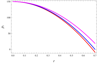
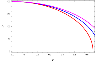
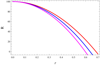
Figure 1: Variation of $p_{r}$, $p_{t}$, $\rho$ and $R$ versus $r$ for $p_{r}=\alpha\rho^{2}$, $\beta=0.5$, $\alpha=0.0025$, $\sigma=2$, $\gamma=30$ (red), $\gamma=35$ (blue) and $\gamma=40$ (magenta).

Figure 1 represents that pressure (radial and tangential) and energy density are maximum at the center and their values decrease with the increase in radial coordinate and increase with the larger values of model parameter $\gamma$. The radial pressure is zero at $r=0.7km$ providing that this is the radius of a polytropic star in this case. The plot of Ricci scalar shows decreasing behavior with the increase in the radius of star while its value also decreases for larger values of the coupling constant.

To investigate the presence of exotic/normal matter distribution in the interior of polytropic star, the energy conditions for anisotropic fluid are defined by [35]

• Null energy condition:  $\rho+p_{r}\geq 0$, $\rho+p_{t}\geq 0$,

• Strong energy condition:  $\rho+p_{r}\geq 0$, $\rho+p_{t}\geq 0$, $\rho+p_{r}+2p_{t}\geq 0$,

• Dominant energy condition:  $\rho\geq|p_{r}|$, $\rho\geq|p_{t}|$,

• Weak energy condition: $\rho\geq 0$, $\rho+p_{r}\geq 0$,  $\rho+p_{t}\geq 0$.

The plots of all energy conditions are given in Figure 2 which indicate that our system of equations corresponding to this case of polytropic EoS is feasible with all the energy conditions for different parametric values of $\gamma$. This analysis also ensures physical viability of our proposed functional form of this gravity.

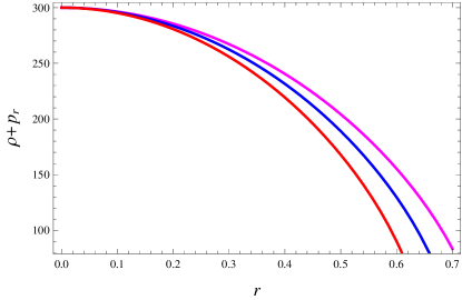
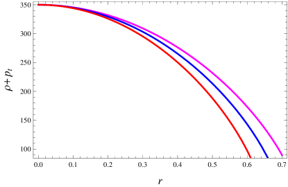
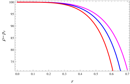
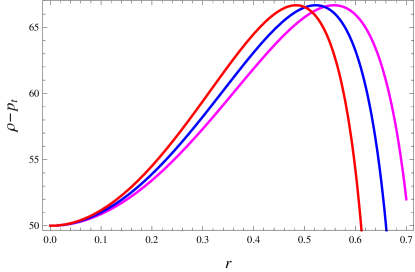
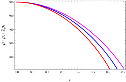
Figure 2: Plots of energy conditions versus radial coordinate for $p_{r}=\alpha\rho^{2}$, $\beta=0.5$, $\alpha=0.0025$, $\sigma=2$, $\gamma=30$ (red), $\gamma=35$ (blue) and $\gamma=40$ (magenta).

In the interior of polytropic star, the effect of anisotropic pressure is examined by the anisotropic factor $\Delta=\frac{2}{r}(p_{t}-p_{r})$. For $p_{t}>p_{r}$, $\Delta>0$ indicating the outward direction of anisotropic pressure while for $p_{t}<p_{r}$, $\Delta<0$ which represents the inward direction of anisotropic pressure. In order to obtain the expression of mass function, the Misner-Sharp formula in GR is given by [36]

$$m=\frac{r}{2}\left(1+g^{ab}r_{,a}r_{,b}\right),$$ (23)

where $m$ represents the gravitational mass within the sphere of radius $r$. For static spherically symmetric spacetime, the expression of mass function in GR is represented as

$$m=\frac{r}{2}\left(1-e^{-\lambda}\right).$$

Replacing this expression in Eq.(11) yields

$$m^{\prime} = \frac{r^{2}}{2(2\sigma R-\gamma\rho)}\left[\rho+\frac{\gamma}{2}R\rho-\frac{\sigma}{2}R^{2}+e^{-\lambda}\left\{\frac{\gamma}{8}\mu^{\prime 2}\rho-\sigma R^{\prime}\left(\lambda^{\prime}-\frac{4}{r}\right)\right.\right.$$

$$+ \left.\left.\gamma p_{r}\left(\frac{\lambda^{\prime}}{r}-\frac{1}{r^{2}}\right)+2\sigma R^{\prime\prime}-\frac{\gamma}{2}\rho^{\prime}\left(\frac{\lambda^{\prime}}{2}-\frac{5\mu^{\prime}}{2}-\frac{2}{r}\right)+\frac{\gamma}{2}\left(\rho^{\prime\prime}-p_{r}^{\prime\prime}\right)\right.\right.$$

$$+ \left.\left.\frac{\gamma}{r}p_{t}^{\prime}-\frac{\gamma}{2}p_{r}^{\prime}\left(\frac{4}{r}-\frac{\lambda^{\prime}}{2}\right)\right\}\right].$$

This equation leads to the following form of mass function

$$m = \frac{1}{2}\int_{0}^{r}\frac{r^{2}}{2\sigma R-\gamma\rho}\left[\rho+\frac{\gamma}{2}R\rho-\frac{\sigma}{2}R^{2}+e^{-\lambda}\left\{\frac{\gamma}{8}\mu^{\prime 2}\rho-\sigma R^{\prime}\left(\lambda^{\prime}-\frac{4}{r}\right)\right.\right.$$ (24)

$$+ \left.\left.\gamma p_{r}\left(\frac{\lambda^{\prime}}{r}-\frac{1}{r^{2}}\right)+2\sigma R^{\prime\prime}-\frac{\gamma}{2}\rho^{\prime}\left(\frac{\lambda^{\prime}}{2}-\frac{5\mu^{\prime}}{2}-\frac{2}{r}\right)+\frac{\gamma}{2}\left(\rho^{\prime\prime}-p_{r}^{\prime\prime}\right)\right.\right.$$

$$+ \left.\left.\frac{\gamma}{r}p_{t}^{\prime}-\frac{\gamma}{2}p_{r}^{\prime}\left(\frac{4}{r}-\frac{\lambda^{\prime}}{2}\right)\right\}\right]dr.$$

This is the Misner-Sharp formula for static spherically symmetric spacetime corresponding to the $\sigma R^{2}+\gamma Q$ model of $f(R,T,Q)$ gravity. For non-static spherically symmetric spacetime, the Misner-Sharp formula in the same gravity is also discussed in [37]. From Eq.(24), we can check the behavior of masses of anisotropic polytropes corresponding to two cases of polytropic EoS with initial condition $m(0)=0$. The mass to radius ratio, also known as compactness factor, is defined as

$$u=\frac{m}{r}.$$

The surface redshift also plays a dynamic role to understand the physics of strong interaction between particles inside the star and its EoS. The formula for $z_{s}$ relative to mass-function is

$$z_{s}=\left(1-\frac{2m}{r}\right)^{-1/2}-1.$$ (25)

The graphical interpretation of $\Delta$, mass-function, compactness factor as well as redshift parameter is presented in Figure 3. The plot of anisotropic factor shows its positive behavior yielding a repulsive force which permits the construction of more massive distribution inside the polytropic star. Figure 3 also illustrates that the value of mass-function remains the same with increasing values of $\gamma$. In this case, the maximum mass point of $0.19M_{\odot}$ is obtained. The maximum value of compactness factor is found to be less than $\frac{4}{9}$. It is also observed that the bound of surface redshift is $z_{s}\leq 5.211$. This analysis shows that the values of $m$, $u$ and $z_{s}$ are in well agreement with the required limits.

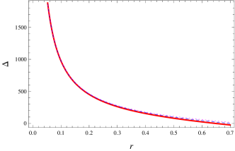
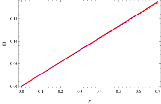
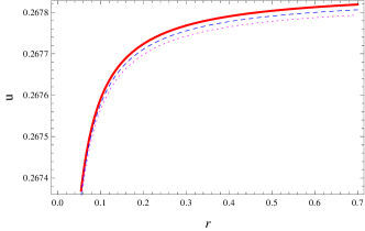
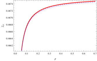
Figure 3: Plots of $\Delta$, $m$, $u$ and $z_{s}$ versus radial coordinate for $p_{r}=\alpha\rho^{2}$, $\beta=0.5$, $\alpha=0.0025$, $\sigma=2$, $\gamma=30$ (red), $\gamma=35$ (blue dashed) and $\gamma=40$ (magenta dotted).

The stability of stellar structure has a great importance in analyzing physically acceptable models. We investigate stability of anisotropic polytropes through analyzing causality condition as well as adiabatic index. According to causality condition, the squared speed of sound defined by $v_{s}^{2}=dp/d\rho$ should lie within the limit $[0,~{}1]$, i.e., $0\leq v_{s}^{2}\leq 1$ everywhere in the interior of stars for a physically stable stellar object. For anisotropic fluid, we have $0\leq v^{2}_{sr}\leq 1$ and $0\leq v^{2}_{st}\leq 1$, where $v_{sr}$ and $v_{st}$ stand for radial as well as transverse components of sound speed, respectively. Herrera [38] introduced the concept of cracking using a different approach to identify potentially stable/unstable structure of compact objects. The potentially stable/unstable regions are computed from the difference of sound speed in radial and transverse directions.

Abreu et al. [39] described the potentially stable and unstable regions as

• $-1\leq v^{2}_{st}-v^{2}_{sr}\leq 0$, for potentially stable region,

• $0\leq v^{2}_{st}-v^{2}_{sr}\leq 1$, for potentially unstable region.

From $\mid v^{2}_{st}-v^{2}_{sr}\mid\leq 1$, we mean that there is no cracking or overturning appears in the system. The adiabatic index also plays a vital role to investigate the stability of relativistic as well as non-relativistic stellar objects. Chandrasekhar [40] and other researchers [41] studied the dynamical stability against infinitesimal radial adiabatic perturbation of the stellar system. It is found that the value of adiabatic index should be greater than $\frac{4}{3}$ in the interior of a dynamically stable stellar object. The expression of adiabatic index for anisotropic fluid is defined by

$$\Gamma_{r}=\frac{\rho+p_{r}}{p_{r}}\left(dp_{r}/d\rho\right),\quad\Gamma_{t}=\frac{\rho+p_{t}}{p_{t}}\left(dp_{t}/d\rho\right).$$ (26)

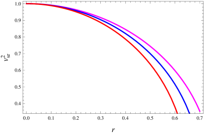
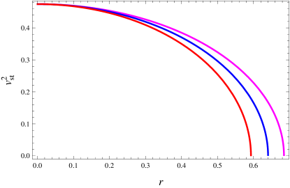
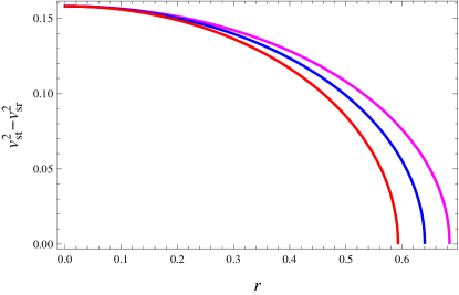
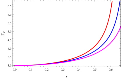
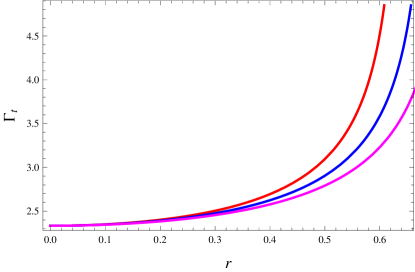
Figure 4: Stability analysis versus radial coordinate for $p_{r}=\alpha\rho^{2}$, $\beta=0.5$, $\alpha=0.0025$, $\sigma=2$, $\gamma=30$ (red), $\gamma=35$ (blue) and $\gamma=40$ (magenta).

Figure 4 represents the graphical behavior of squared speed of sound and adiabatic index for polytropic EoS in this case. This analysis indicates that the anisotropic polytropes are potentially stable and no cracking is observed. It also shows that the system of differential equations is dynamically stable for all values of coupling parameter $\gamma$.

4.2 Case II: $\nu=5/3$

Here we explore the features of anisotropic polytropes considering polytropic EoS $p_{r}=\alpha\rho^{\frac{5}{3}}$. The set of Eqs.(12) and (14)-(16) corresponding to Eq.(17) turns out to be

$$p_{r}^{\prime\prime} = \frac{5\alpha^{\frac{3}{5}}p_{r}^{\frac{2}{5}}}{3+5(1+\beta)\alpha^{\frac{3}{5}}p_{r}^{\frac{2}{5}}}\left[p_{r}^{\prime}\left\{\frac{3}{5\alpha^{\frac{3}{5}}p_{r}^{\frac{2}{5}}}\left(\frac{\lambda^{\prime}}{2}-\frac{5\mu^{\prime}}{2}-\frac{2}{r}\right)-2\beta\left(\frac{\mu^{\prime}}{4}-\frac{\lambda^{\prime}}{4}\right.\right.\right.$$ (27)

$$+ \left.\left.\left.\frac{3}{r}\right)-\frac{3\mu^{\prime}}{2}-\frac{4}{r}+\frac{\lambda^{\prime}}{2}+\frac{6p_{r}^{\prime}}{25\alpha^{\frac{3}{5}}p_{r}^{\frac{7}{5}}}\right\}+p_{r}\left\{\frac{\lambda^{\prime}}{r}-\frac{\mu^{\prime}\lambda^{\prime}}{2}+\frac{\mu^{\prime 2}}{2}+\frac{\beta\mu^{\prime}}{r}\right.\right.$$

$$+ \left.\left.\mu^{\prime\prime}-\frac{2}{\alpha^{\frac{3}{5}}p_{r}^{\frac{2}{5}}}\left(\frac{\mu^{\prime\prime}}{2}+\frac{\lambda^{\prime}}{2r}+\frac{\mu^{\prime}}{2r}-\frac{\mu^{\prime}\lambda^{\prime}}{4}+\frac{e^{\lambda}}{r^{2}}-\frac{1}{r^{2}}+\frac{5\mu^{\prime 2}}{8}\right)-\frac{e^{\lambda}}{\gamma}(2\right.\right.$$

$$+ \left.\left.R)\left(1+\beta+\frac{1}{\alpha^{\frac{3}{5}}p_{r}^{\frac{2}{5}}}\right)\right\}+\frac{4\sigma R}{\gamma}\left(\frac{\mu^{\prime\prime}}{2}+\frac{\lambda^{\prime}}{2r}+\frac{\mu^{\prime}}{2r}-\frac{\mu^{\prime}\lambda^{\prime}}{4}+\frac{e^{\lambda}}{r^{2}}-\frac{1}{r^{2}}\right.\right.$$

$$+ \left.\left.\frac{\mu^{\prime 2}}{4}\right)-\frac{2\sigma R^{\prime}}{\gamma}\left(\frac{2}{r}-\mu^{\prime}\right)\right],$$

$$\lambda^{\prime\prime} = \lambda^{\prime}\left(\frac{4\beta}{r}-\mu^{\prime}-\frac{3\lambda^{\prime}}{2}-\frac{2p_{r}^{\prime}}{p_{r}}+\frac{\mu^{\prime}}{\alpha^{\frac{3}{5}}p_{r}^{\frac{2}{5}}}\right)+e^{\lambda}\left(\frac{2}{r^{2}\alpha^{\frac{3}{5}}p_{r}^{\frac{2}{5}}}-R-\frac{\sigma R^{2}}{\gamma p_{r}}\right.$$ (28)

$$- \left.\frac{2}{\gamma}-\frac{4\sigma R}{\gamma r^{2}p_{r}}\right)+\left(\frac{4\sigma R}{\gamma rp_{r}}-\frac{2}{r\alpha^{\frac{3}{5}}p_{r}^{\frac{2}{5}}}\right)\left(\mu^{\prime}+\frac{1}{r}\right)+\mu^{\prime\prime}-\frac{\mu^{\prime 2}}{\alpha^{\frac{3}{5}}p_{r}^{\frac{2}{5}}}-\frac{2\mu^{\prime}}{r}$$

$$+ p_{r}^{\prime}\left(\frac{3\mu^{\prime}}{5\alpha^{\frac{3}{5}}p_{r}^{\frac{7}{5}}}-\frac{2(1+\beta)}{rp_{r}}-\frac{1}{p_{r}}(\frac{2}{r}+\frac{\mu^{\prime}}{2})\right)+\frac{4\sigma R^{\prime}}{\gamma p_{r}}(\frac{2}{r}+\frac{\mu^{\prime}}{2}),$$

$$\mu^{\prime\prime\prime} = \mu^{\prime\prime}\left(\frac{3\lambda^{\prime}}{2}-\frac{3\mu^{\prime}}{2}-\frac{2}{r}-\frac{p_{r}^{\prime}}{2p_{r}}-\frac{\mu^{\prime}}{2\alpha^{\frac{3}{5}}p_{r}^{\frac{2}{5}}}-\frac{3p_{r}^{\prime}}{10\alpha^{\frac{3}{5}}p_{r}^{\frac{7}{5}}}\right)+\mu^{\prime}\left\{\frac{\lambda^{\prime\prime}}{2}+\frac{2\lambda^{\prime}}{r}\right.$$ (29)

$$- \left.\frac{1}{\gamma}-\frac{\mu^{\prime 2}}{4}-\frac{\lambda^{\prime 2}}{2}+\frac{3\mu^{\prime}\lambda^{\prime}}{4}-R-\frac{1}{\gamma\alpha^{\frac{3}{5}}p_{r}^{\frac{2}{5}}}+\frac{(1+\beta)p_{r}^{\prime}}{rp_{r}}+\frac{2(1+\beta)}{r^{2}}\right.$$

$$- \left.\frac{R}{\alpha^{\frac{3}{5}}p_{r}^{\frac{2}{5}}}+\frac{p_{r}^{\prime}}{4p_{r}}(\lambda^{\prime}-\mu^{\prime})+\frac{1}{\alpha^{\frac{3}{5}}p_{r}^{\frac{2}{5}}}\left(\frac{\mu^{\prime}\lambda^{\prime}}{4}-\frac{\mu^{\prime}}{r}-\frac{\mu^{\prime 2}}{4}\right)-\frac{3p_{r}^{\prime}}{5\alpha^{\frac{3}{5}}p_{r}^{\frac{7}{5}}}\right.$$

$$\times \left.\left(\frac{1}{r}-\frac{\lambda^{\prime}}{4}+\frac{\mu^{\prime}}{4}\right)\right\}-\frac{p_{r}^{\prime}}{p_{r}}\left(\frac{2}{\gamma}+R-\frac{\lambda^{\prime}}{r}\right)+\frac{2\lambda^{\prime\prime}}{r}+\frac{2\lambda^{\prime}}{r^{2}}+\frac{6Rp_{r}^{\prime}}{5\alpha^{\frac{3}{5}}p_{r}^{\frac{7}{5}}}$$

$$+ R^{\prime}\left(3+2\beta-\frac{1}{\alpha^{\frac{3}{5}}p_{r}^{\frac{2}{5}}}\right)-\frac{2\lambda^{\prime 2}}{r}+2(1+\beta)\left\{\frac{2}{r^{3}}-\frac{2e^{\lambda}}{r^{3}}-\frac{\lambda^{\prime}}{r^{2}}-\frac{p_{r}^{\prime}}{p_{r}}\right.$$

$$\times \left.\left(\frac{e^{\lambda}}{r^{2}}-\frac{1}{r^{2}}+\frac{\lambda^{\prime}}{2r}\right)\right\},$$

$$R^{\prime\prime} = \frac{e^{\lambda}p_{r}}{6\sigma}\left\{3+2\beta-\frac{1}{\alpha^{\frac{3}{5}}p_{r}^{\frac{2}{5}}}+\frac{\gamma R}{2}\left(3+2\beta+\frac{1}{\alpha^{\frac{3}{5}}p_{r}^{\frac{2}{5}}}\right)\right\}-R^{\prime}\left(\frac{\mu^{\prime}}{2}+\frac{2}{r}\right.$$ (30)

$$- \left.\frac{\lambda^{\prime}}{2}\right)-\frac{\gamma}{12\sigma}p_{r}^{\prime\prime}\left(\frac{3}{5\alpha^{\frac{3}{5}}p_{r}^{\frac{2}{5}}}-5-2\beta\right)+\frac{\gamma}{12\sigma}p_{r}^{\prime}\left(\frac{7\mu^{\prime}}{2}+\frac{10}{r}-\frac{5\lambda^{\prime}}{2}\right.$$

$$+ \left.\beta(\mu^{\prime}-\lambda^{\prime})+\frac{6p_{r}^{\prime}}{25\alpha^{\frac{3}{5}}p_{r}^{\frac{7}{5}}}+\frac{3}{5\alpha^{\frac{3}{5}}p_{r}^{\frac{2}{5}}}\left(\frac{\lambda^{\prime}}{2}-\frac{2}{r}-\frac{\mu^{\prime}}{2}\right)\right)+\frac{\gamma}{6\sigma}p_{r}\left(\frac{\mu^{\prime\prime}}{2}+\frac{\mu^{\prime}}{r}\right.$$

$$+ \left.\frac{\mu^{\prime 2}}{4}-\frac{\mu^{\prime}\lambda^{\prime}}{4}+\frac{\beta}{r}\left(\lambda^{\prime}-\mu^{\prime}\right)+\frac{1}{\alpha^{\frac{3}{5}}p_{r}^{\frac{2}{5}}}\left(\frac{\mu^{\prime\prime}}{2}-\frac{\mu^{\prime}\lambda^{\prime}}{4}+\frac{\mu^{\prime}}{r}+\frac{3\mu^{\prime 2}}{4}\right)\right).$$

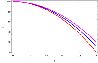
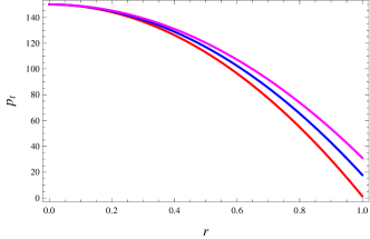
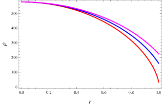
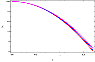
Figure 5: Variation of $p_{r}$, $p_{t}$, $\rho$ and $R$ versus $r$ for $p_{r}=\alpha\rho^{5/3}$, $\beta=0.5$, $\alpha=0.0025$, $\sigma=2$, $\gamma=40$ (red), $\gamma=45$ (blue) and $\gamma=50$ (magenta).

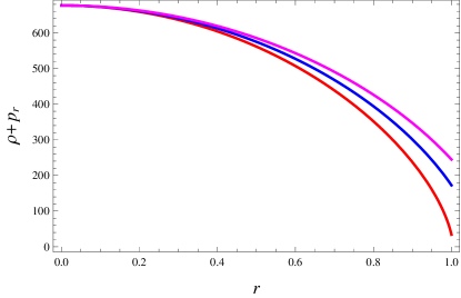
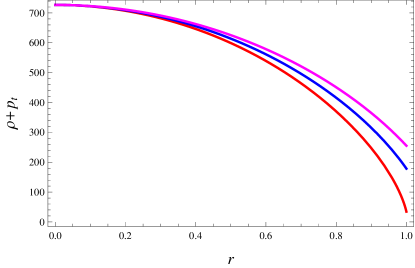
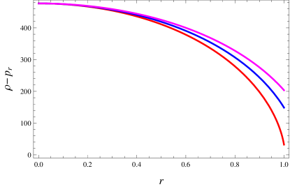
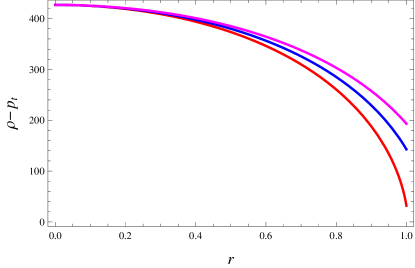
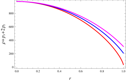
Figure 6: Plots of energy conditions versus radial coordinate for $p_{r}=\alpha\rho^{5/3}$, $\beta=0.5$, $\alpha=0.0025$, $\sigma=2$, $\gamma=40$ (red), $\gamma=45$ (blue) and $\gamma=50$ (magenta).

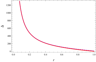
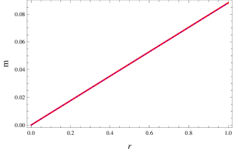
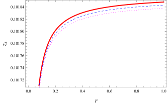
Figure 7: Plots of $\Delta$, $m$, $u$ and $z_{s}$ versus radial coordinate for $p_{r}=\alpha\rho^{5/3}$, $\beta=0.5$, $\alpha=0.0025$, $\sigma=2$, $\gamma=40$ (red), $\gamma=45$ (blue dashed) and $\gamma=50$ (magenta dotted).

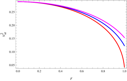
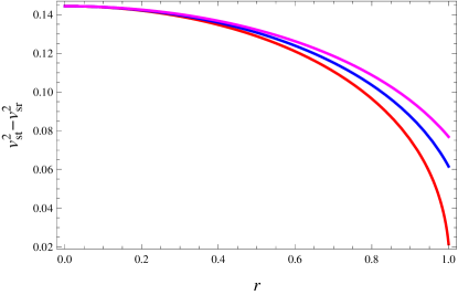
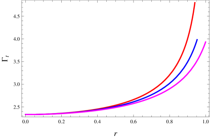
Figure 8: Stability analysis versus radial coordinate for $p_{r}=\alpha\rho^{5/3}$, $\beta=0.5$, $\alpha=0.0025$, $\sigma=2$, $\gamma=40$ (red), $\gamma=45$ (blue) and $\gamma=50$ (magenta).

We solve this system of equations numerically for the same initial conditions, same values of $\alpha$, $\beta$ and $\sigma$ as in the first case while the values of $\gamma$ are changed to obtain the required behavior of density and pressure profiles. The graphs of various physical quantities are plotted in Figures 5-8. The behavior shown in Figure 5 indicates that the radial/tangential pressure, energy density and Ricci scalar possess maximum values at the center that decrease towards the boundary of polytropic star. However, in this case, $p_{r}=0$ at $r=1km$ suggesting that this is the radius of anisotropic polytropes.

Figure 6 reveals that all energy conditions are also satisfied corresponding to the second case of polytropic EoS. For this case, the behavior of anisotropic factor is also positive, maximum mass point of $0.1M_{\odot}$ is found for all values of coupling parameter $\gamma$, the value of compactness factor is found to be less than $\frac{4}{9}$ and the value of gravitational redshift also lies within the observational range as presented in Figure 7. The plots in Figure 8 represent that the radial/tangential components of squared speed of sound lie within the required range throughout the interior of stellar structure. The squared tangential speed of sound is greater than squared radial speed indicating no cracking occurs and $\mid v^{2}_{st}-v^{2}_{sr}\mid\leq 1$ while adiabatic index is greater than $\frac{4}{3}$ implies stable structure of polytropic star.

5 Discussion and Conclusions

The aim of this paper is to explore the basic physical characteristics as well as stability of compact objects for two cases of polytropic EoS in $f(R,T,Q)$ gravity. The analysis of polytropic stars have been observed by constructing equations of stellar structure, hydrostatic equilibrium equation and trace equation under the effect of anisotropic pressure for particular functional form $\sigma R^{2}+\gamma Q$ of this gravity. The hydrostatic equilibrium equation also known as Tolman-Oppenheimer-Volkoff equation, is an extension due to the presence of extra terms coming from $\gamma Q$. The stellar configurations of polytropic stars have been examined for different values of the model parameter $\gamma$.

We have formulated a system of equations and developed the initial conditions required for the numerical analysis. We have considered two polytropic EoS $p_{r}=\alpha\rho^{2}$ and $p_{r}=\alpha\rho^{5/3}$. The regularity conditions for energy density, radial/tangential pressure are satisfied for both cases. It is found that at the center, anisotropic polytropes exhibit maximum pressure and density which decrease monotonically towards the boundary of the star. The radii of approximately $0.7km$ and $1km$ are obtained for cases I and II, respectively. It is found that a large value of coupling parameter $\gamma$ exhibits large radius of the polytropic stars.

Our system of equations is also consistent with all energy conditions corresponding to all chosen values of the model parameter for both cases. The maximum mass points $0.19M_{\odot}$ and $0.1M_{\odot}$ with particular constants and initial conditions are observed for the first and second polytropic EoS, respectively. The maximum values of compactness factor are found 0.26782 for case I and 0.08816 for case II. The maximum gravitational redshift for both cases is $z_{s}\leq 5.211$. We have found that radial/tangential speed of sound for different values of $\gamma$ lie between $[0,~{}1]$ for both polytropic EoS which confirms the stable structure of polytropic stars. The adiabatic index ($\gamma>\frac{4}{3}$) is obtained for both cases which verifies the stability against an infinitesimal radial adiabatic perturbation.

There are bounds on the masses of compact stars in GR. Chandrasekhar [42] suggested maximum mass of $1.4M_{\odot}$ for white dwarfs to produce enough electron degeneracy pressure against collapse whereas Tolman-Oppenheimer-Volkoff [43] limit for the mass of neutron stars is $3M_{\odot}$ to overcome gravity by neutron degeneracy pressure. Also, in [3] the anisotropic polytropes with polytropic exponents 2 and 3/2 are discussed analytically and the maximum mass point of $2.2976M_{\odot}$ for $R=7.07km$ is observed. In [5], the charged polytropic stars are investigated for different polytropic index and for $p_{r}=\alpha\rho^{2}$, the maximum mass of $1.667M_{\odot}$ is obtained. In our scenario, we have found the masses of $0.19M_{\odot}$ and $0.1M_{\odot}$ for the first and second polytropic EoS, respectively which are less than the masses observed in GR.

It is found that the masses, compactness factors and surface redshift of the anisotropic polytropic stars lie within the observational limits in $f(R,T,Q)$ gravity. We have also found that the radii of anisotropic polytropes for $\sigma R^{2}+\gamma Q$ model are very small as compared to radii obtained for polytropic EoS using perfect fluid distribution in $f(R,T)$ gravity [26]. However, these radii are comparable to those obtained for charged polytropic stars corresponding to perfect fluid distribution [27]. We conclude that the effect of anisotropy as well as non-minimal matter-curvature coupling provides a possibility of the existence of such small compact objects.

Acknowledgment

We would like to thank the Higher Education Commission, Islamabad, Pakistan for its financial support through the Indigenous Ph.D. 5000 Fellowship Program Phase-II, Batch-III.

References

- [1] Eicher D.J.: The New Cosmos Answering Astronomy’s Big Questions (Cambridge University Press, 2015).
- [2] Tooper, R.: Astrophys. J. 140(1964)434.
- [3] Thirukkanesh, S. and Ragel, F.C.: Pramana J. Phys. 78(2012)687.
- [4] Herrera, L. et al.: Gen. Relativ. Gravit. 46(2014)1827.
- [5] Ngubelanga, S.A. and Maharaj, S.D.: Eur. Phys. J. Plus 130(2015)211.
- [6] Sharif, M. and Sadiq, S.: Can. J. Phys. 93(2015)1420; ibid. 1583.
- [7] Buchdahl, H.A.: Phys. Rev. 116(1959)1027.
- [8] Ivanov, B.V.: Phys. Rev. D 65(2002)104011.
- [9] Böhmer, G. and Harko, T.: Class. Quantum Grav. 23(2006)6479.
- [10] Capozziello, S.: Int. J. Mod. Phys. D 483(2002)11; Nojiri, S. and Odintsov, S.D.: Phys. Rev. D 68(2003)123512.
- [11] Harko, T. et al.: Phys. Rev. D 84(2011)024020.
- [12] Haghani, Z. et al.: Phys. Rev. D 88(2013)044023.
- [13] Odintsov, S.D. and Sáez-Gómes, D.: Phys. Lett. B 725(2013)437.
- [14] Sharif, M. and Zubair, M.: J. High Energy Phys. 12(2013)079.
- [15] Sharif, M. and Zubair, M.: J. Cosmol. Astropart. Phys. 11(2013)042.
- [16] Ayuso, I., Jiménez, J.B. and Cruz-Dombriz, Á.: Phys. Rev. D 91(2015)104003.
- [17] Sharif, M. and Waseem, A.: Eur. Phys. J. Plus 131(2016)190; Can. J. Phys. 94(2016)1024.
- [18] Baffou, E.H., Houndjo, M.J.S. and Tosssa, J.: Astrophys. Space Sci. 361(2016)376.
- [19] Yousaf, Z., Bhatti, M.Z. and Farwa, U.: Class. Quantum Grav. 34(2017)145002; Eur. Phys. J. C 77(2017)359.
- [20] Sharif, M. and Waseem, A.: Eur. Phys. J. Plus 133(2018)160.
- [21] Sharif, M. and Waseem, A.: Eur. Phys. J. Plus 133(2018)136.
- [22] Henttunen, K., Multamäki, T. and Vilja, I.: Phys. Rev. D 77(2008)024040.
- [23] Orellana, M. et al.: Gen. Relativ. Gravit. 45(2013)771.
- [24] Henttunen, K. and Vilja, I.: Phys. Lett. B 731(2014)110.
- [25] Moraes, P.H.R.S., José D.V.A. and Malheiro, M.: J. Cosmol. Astropart. Phys. 06(2016)005.
- [26] Sharif, M. and Siddiqa, A.: Int. J. Mod. Phys. 27(2018)1850065.
- [27] Sharif, M. and Siddiqa, A.: Eur. Phys. J. Plus 132(2017)529.
- [28] Landau, L.D. and Lifshitz, E.M.: The Classical Theory of Fields (Pergamon Press, 1971).
- [29] Bowers, R.L. and Liang, E.P.T.: Astrophys. J. 188(1974)657; Herrera, L., Ruggeri, G.J. and Witten, L.: Astrophys. J. 234(1979)1094; Dev, K. and Gleiser, M.: Gen. Relativ. Gravit. 34(2002)179.
- [30] Astashenok, A.V., Odintsov, S.D. and de la Cruz-Dombriz, A.: Class. Quantum Grav. 34(2017)205008.
- [31] Tolman, R.C.: Phys. Rev. 55(1939)364.
- [32] Openheimer, J.R. and Volkoff, G.M.: Phys. Rev. 55(1939)374.
- [33] Heintzmann, H. and Hillebrandt. W.: Astron. Astrophys. 38(1975)51.
- [34] Maciel, W.J.: Introduction to Stellar Structure (Springer, 2016).
- [35] Gasperini, M. and Veneziano, G.: Phys. Rept. 373(2003)1.
- [36] Misner C. W. and Sharp D.: Phys. Rev. 136(1964)571.
- [37] Yousaf, Z., Bhatti, M.Z. and Farwa, U.: Mon. Not. R. Astron. Soc. 464(2017)4509.
- [38] Herrera, L.: Phys. Lett. A 165(1992)206.
- [39] Abreu, H., Hernández, H. and Núñez, L.A.: Class. Quantum Grav. 24(2007)4631.
- [40] Chandrasekhar, S.: Astrophys. J. 140(1964)417.
- [41] Hillebrandt, W. and Steinmetz, K.O.: Astron. Astrophys. 53(1976)283; Bombaci, I.: Astron. Astrophys. 305(1996)871.
- [42] Shapiro, S.L. and Teukolsky, S.A.: Black Holes, White Dwarfs and Neu- tron Stars (John Wiley and Sons, 1983).
- [43] Bombaci, I.: Astron. Astrophys. 305(1996)871.