Circular Motion and Energy Extraction in a Rotating Black Hole

Abstract

This paper explores the circular geodesics of neutral test particles on an equatorial plane around a rotating black hole. After using equations of motion of scalar-tensor-vector gravity with the circular geodesics of null-like particles, we find the equation of photon orbit. With the help of an effective potential form, we have examined the stable regimes of photons orbits. The Lyapunov exponent, as well as the effective force acting on photons, is also investigated. We examine the energy extraction from a black hole via Penrose process. Furthermore, we discuss the negative energy state and the efficiency of energy extraction. We have made compare our results with that obtained for some well known black holes models. We concluded that the efficiency of the energy extraction decreases with the increase of dimensionless parameter of theory and increases as spin parameter increases.

Keywords: Black hole physics, Gravitation, Geodesics.

1 Introduction

The process of exploring the hidden aspects of our Cosmos has always been a source of great attractions for many researchers. Different Cosmic data-sets indicate that our Universe is undergoing accelerated expansion phase that has opened up new directions. It is believed that this expansion is due to an enigmatic force, dubbed as dark energy (DE). Apart from that, the dynamics of another mysterious matter need to explore which is widely known as dark matter (DM). Such a matter has no interaction with the light and electromagnetic force. Modified gravity theories are useful to reveal the incomprehensible nature of DE as well as DM. These theories are the modification of the usual Einstein gravity (for further reviews on DE and modified gravity, see, for instance, [1, 2, 3, 4]). Moffat [5] proposed scalar-tensor-vector gravity (STVG) as one of the models that could be considered as an alternative for DM. In the action of this modified theory of gravity (MOG), field for three scalars and massive vector are included along with the Einstein-Hilbert term and the matter action. This theory is useful to discuss the rotational curves of galaxies, solar system, gravitational lensing of galaxy, motion of galaxy clusters without considering DM [8].

Moffat and Rahvar [9] studied some dynamical features of galaxy clusters in the gravity by applying weak-filed approximations. Moffat [10] studied the shadows of black holes (BHs) in the same theory and found that size of the shadows increases as the parameter $\alpha$ increases. Mureika et al. [11] discussed the thermodynamics of MOG-BHs and found that the entropy area law changes as $\alpha$ increases. Lee and Han [12] investigated that radius of the inner most stable circular orbit for Kerr-MOG BH increases with the increasing values of $\alpha$. Sharif and Shahzadi [13] analyzed the effects of magnetic field on the particle dynamics for timelike geodesics around Kerr-MOG BH. A useful result on the the investigation of null geodesics in the background of MOG is produced by Rahvar and Moffat [14]. They analyzed the propagation of electromagnetic waves in MOG and calculated the corresponding deflection angle. They found quite larger bending angle of light in MOG as compared to that obtained in general relativity.

In recent years, the motion of particles (massless or massive) near a BH remained a compelling issue in BH astrophysics. The study of geodesics reveals the geometrical structure as well as the important features of a curved spacetime. They also help to determine the gravitational field around a BH. Among various types of geodesics, the most fascinating one is circular geodesics. The circular geodesic motion of particles for Schwarzschild, Reissner-Nordström as well as Kerr BHs has been discussed [15]. Bardeen [16] studied the properties of a Kerr BH and its circular orbits. Pugliese and Quevedo [17] identified the regions inside the ergoregion of Kerr BH and deduce that distribution of circular orbits depends on the rotation parameter of a source.

A physical particle follows either timelike or null geodesics. The study of circular null orbits is important from both theoretical and astrophysical points of view. Frolov and Stojkovic [18] analyzed the particle as well as light motion and concluded that there are no stable circular orbits in an equatorial plane around a five-dimensional rotating BH. Konoplya [19] studied the motion of both massive and massless particles near magnetized BHs and found that tidal force has strong effect on particle motion. Fernando [20] investigated that the circular orbits of photons around Schwarzschild BH are more stable than for a BH surrounded by quintessence matter. Khoo and Ong [21] investigated that there cannot be any photon orbit on the event horizon of a non-extremal Kerr-Newman BH. Pradhan [22] explored null circular geodesics near Ayón-Beato-García BH and found that at a certain radius, there exists zero angular momentum orbits. Yousaf and Bhatti [23] studied the stable regions of some relativistic compact structures in MOG.

Stuchlík et al. [24] studied the particle collision and circular geodesics in the braneworld mining Kerr-Newman naked singularity spacetimes and found that the radius of stable circular photon orbit is almost independent of the spin parameter $a$, being situated nearly to the limiting radius $r=b$, (where $b$ is the tidal charge parameter) and this radius corresponds to the radius of innermost stable circular orbit. They also concluded that there exist an infinitely deep gravitational well centered at the stable photon circular orbit.

Energy extraction from a rotating BH is one of the most important and interesting issues in general relativity as well as in astrophysics. Penrose [25] demonstrated a highly efficient mechanism to extract the energy from a rotating BH and related to the existence of negative energy in the ergoregion. Nozawa and Maeda [26] deduced that more energy can be extracted from higher dimensional BHs as compared to the energy extortion from $4D$ Kerr BH. Pradhan [27] examined the Penrose process near Kerr-Newman-Tab-NUT BH and presented a relation between gained energy and the corresponding NUT parameter. Mukherjee [28] explored the collisional Penrose process using spinning particles around Kerr BH and found that the energy extraction is high in comparison with the non-spinning case.

The efficiency of energy extraction from a rotating BH by Penrose process is defined as (gain in energy)/(input energy). Bhat et al. [29] showed that the efficiency of Penrose process near Kerr-Newman BH gets reduced due to the vicinity of charge in comparison with the the maximum efficiency limit of $20.7\%$ for the Kerr BH. Liu et al. [30] deduced that the deformation parameter increase the efficiency of energy extraction process in the non-Kerr BH. Toshmatov et al. [31] studied Penrose process around rotating regular BH and found that efficiency of energy extraction decreases for increasing values of electric charge. Liu and Liu [32] explored the Penrose process using spinning particles around extremal Kerr BH and concluded that efficiency of the energy extraction monotonously increases with the increase of particle’s spin.

In this paper, we explore the circular geodesic motion and energy extraction by Penrose process in the background of Kerr-MOG BH. In section 2, we introduce the Kerr-MOG BH and study the null geodesics. We derive the equation for circular photon orbits and discuss the stability of these orbits through effective potential. The Lyapunov exponent and the effective force acting on photons is also discussed. Section 3 is devoted to investigate the negative energy state as well as the efficiency of energy extraction via Penrose process. Finally, we summarize our results in last section.

2 Equatorial Circular Geodesics

In this section, we explore the geodesic motion of neutral particles near Kerr-MOG BH which can be characterized by the angular momentum $J=Ma$, mass $M$ as well as the dimensionless parameter $\alpha$ [33]. The spacetime geometry corresponding to this BH can be described by the metric with Boyer-Linquist coordinates

$$ds^{2} = -\frac{\Delta}{\rho^{2}}(dt-a\sin^{2}\theta d\phi)^{2}+\frac{\sin^{2}\theta}{\rho^{2}}\left[(r^{2}+a^{2})d\phi-adt\right]^{2}$$ (1)

$$+ \frac{\rho^{2}}{\Delta}dr^{2}+\rho^{2}d\theta^{2},$$

with

$$g_{tt} = -\left(\frac{\Delta-a^{2}\sin^{2}\theta}{\rho^{2}}\right),\quad g_{rr}=\frac{\rho^{2}}{\Delta},\quad g_{\theta\theta}=\rho^{2},$$

$$g_{\phi\phi} = \frac{\sin^{2}\theta}{\rho^{2}}\left[(r^{2}+a^{2})^{2}-\Delta a^{2}\sin^{2}\theta\right],$$

$$g_{t\phi} = \frac{a\sin^{2}\theta}{\rho^{2}}\left[\Delta-(r^{2}+a^{2})\right].$$

where

$$\Delta=r^{2}+a^{2}-2GMr+\alpha G_{N}GM^{2},\quad\rho^{2}=r^{2}+a^{2}\cos^{2}\theta,$$

here $G=G_{N}(1+\alpha)$ is the gravitational constant, $G_{N}$ is the Newton’s gravitational constant. Moreover, $\alpha$ is introduced to analyze the strength of the gravitational interaction. It is worthy to state that the gravitational source charge of the (spin 1 graviton) vector field $\phi_{\mu}$ is $Q_{g}=\sqrt{\alpha G_{N}}M$. Inserting the value of $G$ in $\Delta$ and using $r\rightarrow r/G_{N}M$, $a\rightarrow a/G_{N}M$ and $\alpha\rightarrow\alpha/G_{N}M$, we obtain

$$\Delta=r^{2}+a^{2}-2(1+\alpha)r+\alpha(1+\alpha).$$

The Kerr-MOG BH is asymptotically flat, axially and stationary symmetric solution of MOG field equations. This has the form of a Kerr-Newman solution of Einstein-Maxwell equations that illustrates the geometry of a spacetime in the background of a rotating and electrically charged body. The metric of Kerr-MOG BH is identical to Kerr-Newman BH with replacement of $\alpha$ by $Q^{2}$, where $Q$ is the electric charge of Kerr-Newman BH. For $\alpha=0$ and $a=0$, the metric (1) boils down to the Kerr and Schwarzschild-MOG metric, respectively. Moreover, the zero choices of both of these parameters describes the Schwarzschild spacetime. On substituting $\Delta=0$, the horizons of Eq.(1) are found to be

$$r_{\pm}=(1+\alpha)\pm\sqrt{1+\alpha-a^{2}},$$

where $\pm$ sign corresponds to the inner and outer horizons, respectively. Figure 1 depicts the horizon structure of Kerr-MOG, Kerr and Schwarzschild-MOG BH. The left graph indicates that the horizon of Kerr-MOG BH is greater than that of Kerr BH. Furthermore, Kerr-MOG BH horizon increases in size with the increasing value of parameter $\alpha$. The right graph shows that the horizon of Schwarzschild-MOG BH is larger in comparison with the Kerr-MOG BH.

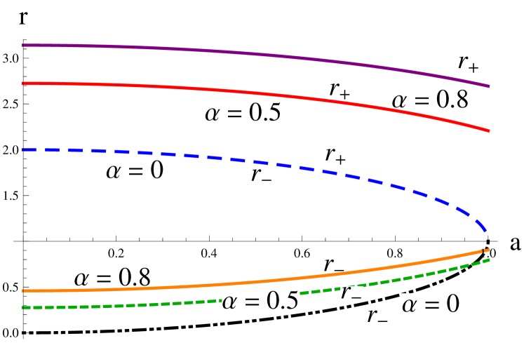
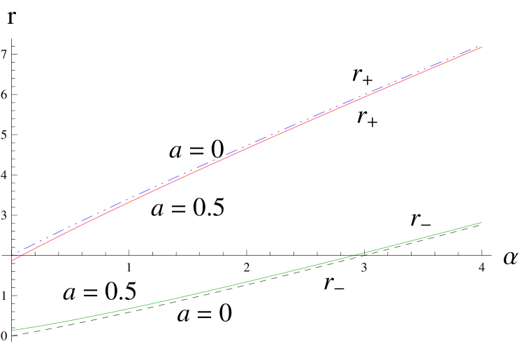
Figure 1: Plots of horizon as a function of $a$ (left) and $\alpha$ (right).

The ergosphere can be calculated by $g_{tt}=0$ as

$$r_{es}=\frac{1}{2}[2(1+\alpha)\pm\sqrt{4-2a^{2}+4\alpha-2a^{2}\cos 2\theta}].$$

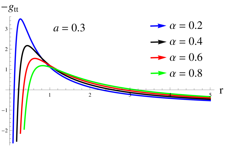
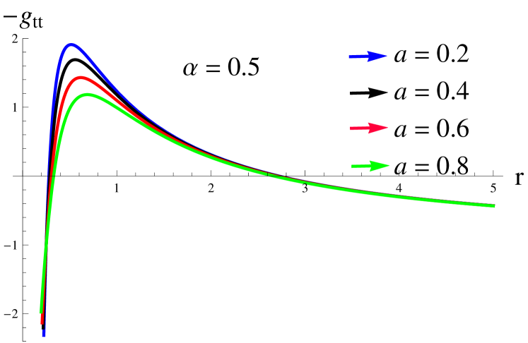
Figure 2: Plots of $-g_{tt}$ as a function of $r$.

For $\theta=0,\pi$, both event horizon and ergosphere coincide. Figure 2 illustrates the nature of the variation of $-g_{tt}$ with respect to the radial coordinate $r$. We observe that the shape of the ergoregion gets modified for increasing values of the spin parameter $a$ as well as $\alpha$ and becomes constant at a larger radial distance $r$.

We consider the circular motion of test particles in the background of Kerr-MOG BH and restrict ourselves to the case of orbits situated on an equatorial plane ($\theta=\pi/2$). The test particle action can be written as [5]

$$S=-\left(m\int d\tau+\lambda\int\omega d\tau\phi_{\mu}\frac{dx^{\mu}}{d\tau}\right),$$ (2)

where $m$ is the mass of the particle, $\lambda$ is the coupling constant and $\tau$ is the proper time of the test particle. Using stationary condition $\delta S/\delta x^{\mu}=0$ in the above equation, the equation of motion for massive particle can be found as [6]

$$\frac{d^{2}x^{\mu}}{d\tau^{2}}+\Gamma^{\mu}_{\nu\beta}\frac{dx^{\nu}}{dx^{\tau}}\frac{dx^{\beta}}{dx^{\tau}}=\frac{q}{m}B^{\mu}_{\sigma}\frac{dx^{\sigma}}{d\tau},$$ (3)

where $\Gamma^{\mu}_{\nu\beta}$ denotes the Christoffel symbols, $q=\sqrt{\alpha G_{N}}M$ is the test particle gravitational charge and $B_{\mu\sigma}=\partial_{\mu}\phi_{\sigma}-\partial_{\sigma}\phi_{\mu}$. The equation of motion for the photon is

$$\frac{d^{2}x^{\mu}}{d\tau^{2}}+\Gamma^{\mu}_{\nu\beta}\frac{dx^{\nu}}{dx^{\tau}}\frac{dx^{\beta}}{dx^{\tau}}=0.$$ (4)

The radial equation of motion for a test particle in an equatorial plane for Kerr-MOG BH can be written as [7]

$$A(r,\alpha)E^{2}-2B(r,L,\alpha)E+C(r,L,\alpha)+r^{4}(p^{r})^{2}=0,$$ (5)

where $p^{r}$ is the radial momentum, $E$ and $L$ denotes the energy and angular momentum of test particle, and

$$A(r,\alpha) = (r^{2}+a^{2})^{2}-\Delta^{2}a^{2},$$

$$B(r,L,\alpha) = (La+r\alpha)(r^{2}+a^{2})-La\Delta,$$

$$C(r,L,\alpha) = (La+r\alpha)^{2}-L^{2}\Delta-r^{2}\Delta.$$

In the following, we discuss the null geodesics, stability of circular photons orbits, effective force and Lyapunov exponent.

2.1 Null Geodesics

For null geodesics, the radial equation can be written as

$$\dot{r}^{2} = E^{2}+\frac{1}{r^{4}}(2(1+\alpha)r-\alpha(1+\alpha))(aE-L)^{2}$$ (6)

$$+ \frac{1}{r^{2}}(a^{2}E^{2}-L^{2}),$$

where dot denotes the derivative with respect to $\tau$. It could be worthwhile to introduce the impact parameter $D=L/E$ instead of $L$. Now, we consider a particular choice, i.e., $L=aE$ for which $D=a$. Thus, the equations for $\dot{t}$, $\dot{\phi}$ and $\dot{r}$ can be written as

$$\dot{t}=\frac{E\left(r^{2}+a^{2}\right)}{\Delta},\quad\dot{\phi}=\frac{Ea}{\Delta},\quad\dot{r}=\pm E,$$

where $\pm$ sign correspond to the outgoing and incoming photons, respectively. The radial coordinate $r$ is specified with respect to affine parameter while the equations for $t$ and $\phi$ are

$$\frac{dt}{dr}=\pm\frac{\left(r^{2}+a^{2}\right)}{\Delta},\quad\frac{d\phi}{dt}=\pm\frac{a}{\Delta}.$$

Now, we examine the general case $L\neq aE$ and determine the radius of unstable photon orbit for which $E=E_{c}$, $L=L_{c}$ and $D_{c}=L_{c}/E_{c}$. Therefore, Eq.(6) and its derivative takes the form

$$r_{c}^{2} + \left(\frac{2(1+\alpha)r_{c}-\alpha(1+\alpha)}{r_{c}^{2}}\right)\left(a-D_{c}\right)^{2}$$ (7)

$$+ \left(a^{2}-D_{c}^{2}\right)=0,$$

$$r_{c}-\left(\frac{(1+\alpha)r^{2}_{c}-\alpha(1+\alpha)r_{c}}{r_{c}^{4}}\right)\left(a-D_{c}\right)^{2}=0.$$ (8)

The last equation implies that

$$D_{c}=a\mp\sqrt{\frac{r_{c}^{5}}{(1+\alpha)r^{2}_{c}-\alpha(1+\alpha)r_{c}}}.$$ (9)

Substituting Eq.(9) into Eq.(7), we obtain

$$r_{c}^{3} - 3(1+\alpha)r^{2}_{c}+2\alpha(1+\alpha)r_{c}$$ (10)

$$\pm 2a\sqrt{r_{c}((1+\alpha)r^{2}_{c}-\alpha(1+\alpha)r_{c})}=0.$$

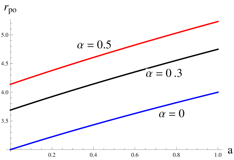
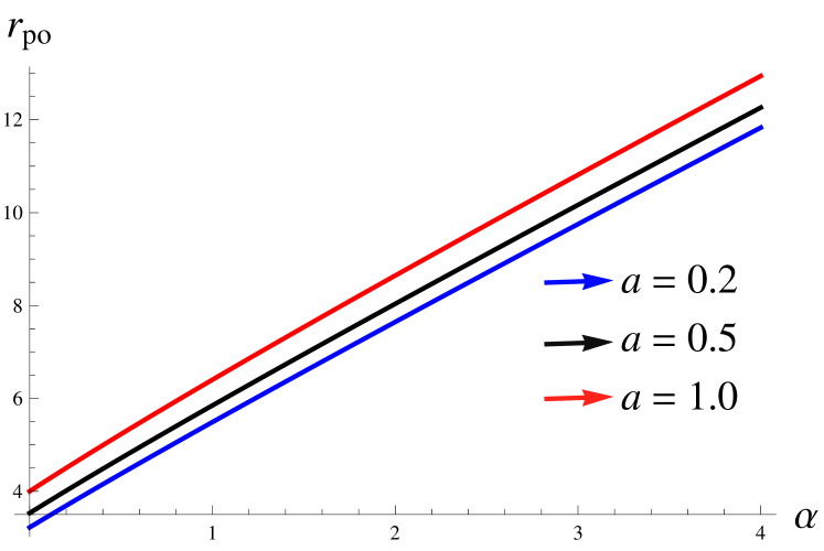
Figure 3: Plots of photon orbit for retrograde motion as a function of $a$ (left) and $\alpha$ (right).

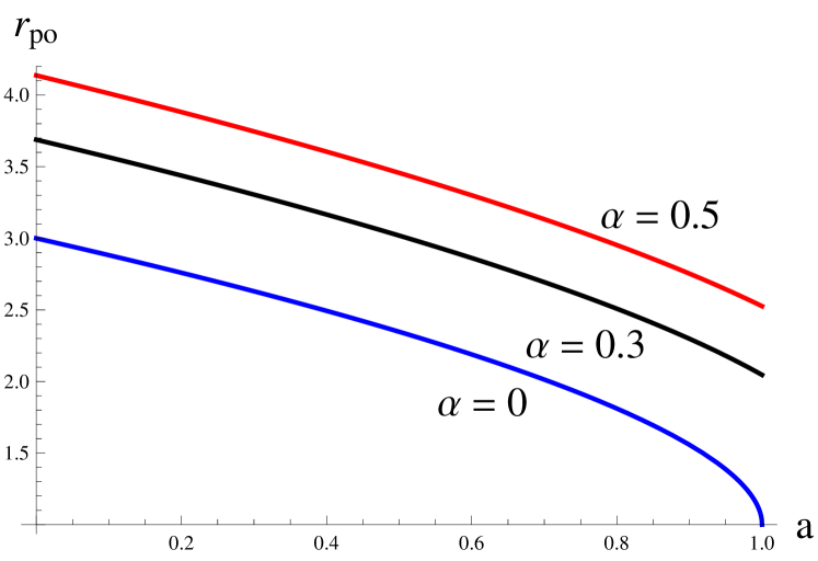
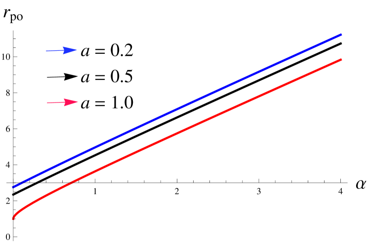
Figure 4: Plots of photon orbit for prograde motion as a function of $a$ (left) and $\alpha$ (right).

Let $r_{c}=r_{po}$ be the real positive root of Eq.(10) which gives radius of the photon orbit for Kerr-MOG BH. It is the closest possible boundary of circular orbits for particles. For $\alpha=a=0$, we obtain Schwarzschild limit ($r_{po}=3M$), while for $\alpha=0$ and $a=1$, we recover the photon orbit of Kerr BH ($r_{po}=M$) [16]. The behavior of photon orbit for different values of $a$ (left) and $\alpha$ (right) for retrograde and prograde motion is depicted in Figures 3 and 4, respectively. Here, we observe that the radius of photon orbit of Kerr-MOG BH is greater in comparison with the Kerr BH and increases for increasing values of $\alpha$ as well as $a$ for retrograde motion. But for prograde motion, the radius of photon orbit increases with the increase of $\alpha$ and decreases as the rotation of a BH increases. From Eqs.(7) and (9), we have

$$D_{c}^{2}=a^{2}+r_{c}^{2}\left[\frac{3(1+\alpha)r^{2}_{c}-2\alpha(1+\alpha)r_{c}}{(1+\alpha)r^{2}_{c}-\alpha(1+\alpha)r_{c}}\right].$$

We can obtain the angular velocity (physical quantity related with the null circular geodesics) measured by asymptotic observer denoted by $\Omega_{c}$ as

$$\Omega_{c} = [(r_{c}^{2}-2(1+\alpha)r_{c}+\alpha(1+\alpha))D_{c}+(2(1+\alpha)r_{c}$$

$$- \alpha(1+\alpha))a][(r_{c}^{2}(r_{c}^{2}+a^{2})+a^{2}(2(1+\alpha)r_{c}-\alpha$$

$$\times (1+\alpha)))-a(2(1+\alpha)r_{c}-\alpha(1+\alpha))D_{c}]^{-1}$$

$$= \frac{1}{D_{c}}.$$

We can see from Eqs.(7) and (9) that the angular frequency of null geodesics is inverse of the impact parameter, which generalize the results of Kerr BH [15] to the Kerr-MOG BH.

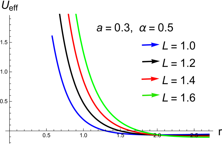
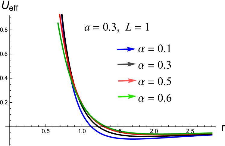
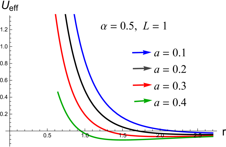
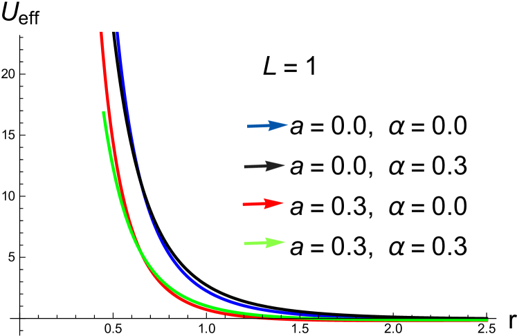
Figure 5: Plots of effective potential versus $r$.

The stability of circular orbits can be illustrated through effective potential ($U_{eff}$). The minimum and maximum values of $U_{eff}$ determine the stable and unstable circular orbits, respectively, while the extreme values of $U_{eff}$ correspond to $U_{eff},r=0$. Equation (6) can be written as [34]

$$\dot{r}^{2} = E^{2}-U_{eff},$$

where

$$U_{eff} = \frac{1}{r^{4}}\left(\alpha(1+\alpha)-2(1+\alpha)r\right)\left(aE-L\right)^{2}$$ (11)

$$- \frac{1}{r^{2}}(a^{2}E^{2}-L^{2}).$$

For a particle to describe a circular orbit (at a constant radius $r=r_{0}$), the initial radial velocity and radial acceleration must be zero. Therefore, we have

$$U_{eff}|_{r=r_{0}},\quad\frac{\partial U_{eff}}{\partial r}|_{r=r_{0}}=0.$$

For stable circular orbits, effective potential must be minimum, i.e.,

$$\frac{\partial^{2}U_{eff}}{\partial r^{2}}|_{r=r_{0}}>0.$$

The behavior of effective potential for null-like particles moving around Kerr-MOG BH is shown in Figure 5. We have varied different choices of angular momentum in this structure and shown our results in the upper portion of the left graphs. It is noticed that the instability of circular photon orbits increases with the increase of angular momentum and at a larger radial distance, does not change much more. The right graph presents that the presence of parameter $\alpha$ contributes to decrease the stability of circular photons orbits. The underneath part of the left diagram indicates more unstable photons circular orbits for large choices of $a$ as compared to smaller ones. The motion of particles become unstable for higher values of $a$. The photons orbits around Kerr-MOG BH are unstable in comparison with the Kerr BH as shown in the right diagram.

2.2 Effective Force

The force that could describe the motion of information, e.g., whether it is directed away or attracted towards the BH, could termed as an effective force. One can obtain effective force acting on the photon using Eq.(11) as [20]

$$F = \frac{-1}{2}\left(\frac{dU_{eff}}{dr}\right)$$

$$= -\frac{(1+\alpha)}{r^{4}}(aE-L)^{2}+\frac{1}{r^{3}}(a^{2}E^{2}-L^{2})$$

$$+ \frac{2(aE-L)^{2}}{r^{5}}\left(2r(1+\alpha)-\alpha(1+\alpha)\right).$$

We see that the first term is attractive while the second term is repulsive if $aE>L$. The third term is also repulsive if $2r(1+\alpha)>\alpha(1+\alpha)$. The graphical analysis of effective force is analyzed in Figure 6. The top portion of the left diagram presents relatively greater attraction on photons by the effective force with higher choices of spin parameter $a$ and at a larger radial distance does not change much more as $a$ increases. The behavior of the effective force with various $\alpha$ choices is depicted in the right diagram. This states the increment on the influence of effective force with respect to the increasing $\alpha$ values and has no effects as the photons move away from the BH. The lower graph gives the comparison of the effective force acting on a photon around the Kerr-MOG BH with the Schwarzschild and Kerr structures. One can observe the more attractive behavior of effective force on a photon for Kerr-MOG BH than that of Schwarzschild and Kerr BHs.

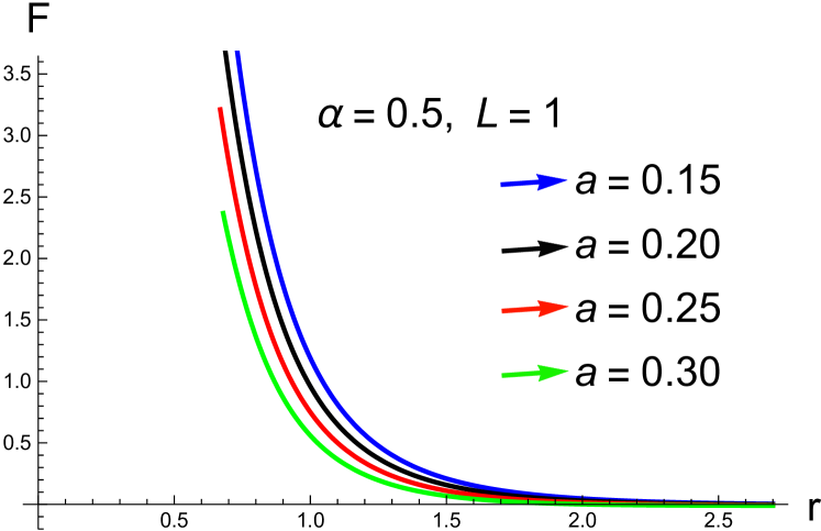
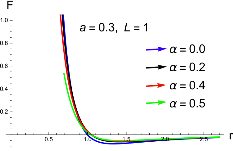
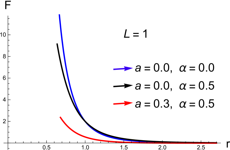
Figure 6: Plots of effective force versus $r$.

2.3 Lyapunov Exponent

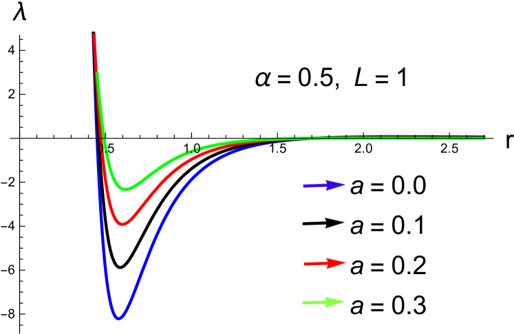
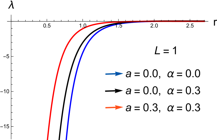
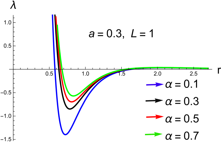
Figure 7: Plots of Lyapunov exponent versus $r$.

The average contraction and expansion geodesics rates can be calculated in a phase space through Lyapunov exponent. The negative and positive Lyapunov exponents determines the convergence and divergence between nearby orbits. After making use of Eq.(11), the Lyapunov exponent for null geodesics has been found to be [35]

$$\lambda = \sqrt{\frac{-U_{eff}^{\prime\prime}(r_{c})}{2\dot{t}^{2}(r_{c})}}$$

$$= [\frac{1}{2L^{2}r^{6}}(aE-L)(\alpha+(r-2)r)(10\alpha^{2}(L-aE)$$

$$+ 2\alpha(6r-5)(aE-L)+3r(aE(r+4)$$

$$+ L(r-4)))]^{\frac{1}{2}}\mid_{r=r_{c}}.$$

In the upper portion of Figure 7, the left diagram describes more unstable circular orbits for large choices of $a$, which indicates the decreasing behavior of Lyapunov exponent with bigger selection of $a$. However, the right diagram indicates that the Lyapunov exponent for Kerr-MOG BH has larger values as compared to Schwarzschild and Schwarzschild-MOG structures. We have plotted lower portion of the diagram for various distinct choices of $\alpha$. We noticed that initially $\lambda$ has decreasing behavior for higher values of $\alpha$ and then increases with the increase of $r$ but does not change much more at a larger radial distance.

3 Energy Extraction by Penrose Process

The energy extraction process from BHs is the momentous problem of general relativity. There are different mechanisms which are devoted to study the energy extraction from rotating BHs. Among these processes, the Penrose process is of great interest and even more efficient than the nuclear reactions. In this process, a particle with positive energy enters into the ergosphere (the region between outer horizon and stationary limit), splitted into two fragments, one of them follows a negative energy orbit while the other escapes to infinity having energy greater than that of the incident particle. If the particles are involved in Penrose process then the necessary and sufficient condition to extract energy is the absorption of particles with negative energies as well as angular momentum. In the following, we study the negative energy state as well as efficiency of energy extraction by the Penrose process around Kerr-MOG BH.

3.1 The Negative Energy State

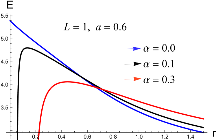
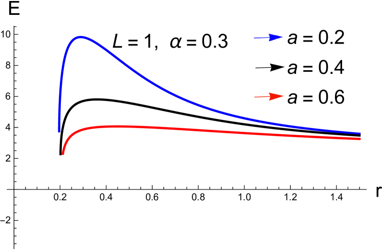
Figure 8: Plots of negative energy as a function of $\alpha$ (left) and $a$ (right).

The negative energy inside the ergosphere has an important consequences in BH physics. It may allows the Penrose process and occur due to the electromagnetic interaction and the counter rotating orbits around BH. Thus, it is useful to find the limits on energy which a particle can have at a particular location. Using Eq.(5), we have

$$E^{2}[r^{2}(r^{2} + a^{2})+a^{2}(2(1+\alpha)r-\alpha(1+\alpha))]-2E(aL(2(1+\alpha)r$$ (12)

$$- \alpha(1+\alpha))+\alpha r(r^{2}+a^{2}))-L^{2}(r^{2}-2(1+\alpha)r$$

$$+ \alpha(1+\alpha))+\alpha r(\alpha r+2aL)-r^{2}\Delta=0.$$

Solving the above equation for $E$ and $L$, we obtain

$$E = \frac{aL(2(1+\alpha)r-\alpha(1+\alpha))\pm\sqrt{X_{1}}}{r^{4}+a^{2}(r^{2}+2(1+\alpha)r-\alpha(1+\alpha))},$$ (13)

$$L = \frac{-aE(2(1+\alpha)r-\alpha(1+\alpha))\pm\sqrt{X_{2}}}{(r^{2}-2(1+\alpha)r+\alpha(1+\alpha))},$$ (14)

where

$$X_{1} = -a^{2}\Delta^{2}(4a^{2}+3L^{2})-3(a^{2}+r^{2})^{2}(aL+\alpha r)^{2}+2\Delta(2a^{6}+a^{4}(3L^{2}$$

$$+ 4r^{2})+3\alpha a^{3}Lr+a^{2}r^{2}(3L^{2}+2(\alpha^{2}+r^{2}))-\alpha aLr^{3}+2L^{2}r^{4}),$$

$$X_{2} = \alpha r(a^{2}+r^{2})+E^{2}(a^{2}(-\alpha(\alpha+1)+r^{2}+2(\alpha+1)r)+r^{4})+4a^{2}$$

$$\times (E(\alpha+1)(\alpha-2r)+\alpha r)^{2}+\alpha^{2}+4\Delta r^{2}(\alpha^{2}+\alpha+r^{2}-2(\alpha+1)r).$$

From Eq.(13), we can inferred the conditions for which energy can be negative. Firstly, we assign an energy $E=1$ to the particle with unit mass, at rest at infinity. We consider $+$ sign of Eq.(13) which requires for $E<0$, $L<0$ and

$$\left(aL\left(2\left(1+\alpha\right)r-\alpha\left(1+\alpha\right)\right)+\alpha r(r^{2}+a^{2})\right)^{2}>X_{1}.$$

Using Eq.(15), the above inequality can be written as

$$\left[r^{4}+a^{2}\left(r^{2}+2\left(1+\alpha\right)r-\alpha(1+\alpha)\right)\right][(r^{2}$$

$$-2(1+\alpha)r+\alpha(1+\alpha))L^{2}-\epsilon r^{2}\Delta]<0.$$

It follows from the above inequality that $E<0$ if and only if $L<0$ and

$$\left(\frac{r^{2}-2(1+\alpha)r+\alpha(1+\alpha)}{r^{2}}\right)<\frac{\epsilon\Delta}{L^{2}}.$$

We observe that on an equatorial plane, only counter rotating particles can have negative energy and particle must be inside the ergosphere ($r<a+M$). In the Penrose process, orbit of particle having negative energy inside the ergosphere is a key to extract the energy from Kerr-MOG BH. Figure 8 describes the negative energy state for different values of $\alpha$ (left) as well as $a$ (right). It is observed that negative energy decreases with the increasing values of parameter $\alpha$. It is interesting to note that negative energy decreases when a BH rotates rapidly.

3.2 Efficiency of Energy Extraction

The efficiency of the energy extraction via Penrose process is one of the most important issues in the energetics of BHs. We assume that a particle with energy $E_{0}$ enters into the ergosphere of BH and splitted into two pieces (namely $1$ and $2$ with energies $E_{1}$ and $E_{2}$, respectively). The piece $1$ has greater energy than the incident particle and leaves the ergosphere while second piece with negative energy falls into the BH. According to the law of conservation of energy

$$E_{0}=E_{1}+E_{2},$$

where $E_{2}<0$, then $E_{1}>E_{0}$. Let $\Omega=\frac{d\phi}{dt}$ and $\upsilon=\frac{dr}{dt}$ represents the angular and the radial velocity of a particle with respect to an asymptotic infinity observer, respectively. From the laws of conservation of energy and angular momentum, we obtain

$$E=-p^{t}\chi,\quad L=p^{t}\Omega,$$ (15)

where

$$\chi\equiv g_{tt}+g_{t\phi}\Omega.$$

Using $p^{\sigma}p_{\sigma}=-m^{2}$, we can obtain

$$g_{tt}\dot{t}^{2}+2g_{t\phi}\dot{t}\dot{\phi}+g_{rr}\dot{r}^{2}+g_{\phi\phi}\dot{\phi}^{2}=-m^{2}.$$

Dividing the above equation by $\dot{t}^{2}$, we have

$$g_{tt}+2g_{t\phi}\Omega+\frac{r^{2}}{\Delta}\upsilon^{2}+g_{\phi\phi}\Omega^{2}=-\left(\frac{m\chi}{E}\right)^{2}.$$ (16)

As the right hand side of above equation is negative or equal to zero and third term in the left hand side is always positive. So, we can write the above equation in the following form

$$g_{tt}+2g_{t\phi}\Omega+g_{\phi\phi}\Omega^{2}=-\left(\frac{m\chi}{E}\right)^{2}-\frac{r^{2}}{\Delta}\upsilon^{2}\leq 0.$$

The angular velocity $\Omega$ must be in the range of $\Omega_{-}\leq\Omega\leq\Omega_{+}$ [26], where

$$\Omega_{\pm}=-\frac{g_{t\phi}}{g_{\phi\phi}}\pm\sqrt{\frac{g^{2}_{t\phi}-g_{tt}g_{\phi\phi}}{g^{2}_{\phi\phi}}}.$$

Using Eq.(15), the equations of conservation of energy and angular momentum can be written as

$$p^{t}_{(0)}\chi_{(0)}=p^{t}_{(1)}\chi_{(1)}+p^{t}_{(2)}\chi_{(2)},$$ (17)

$$p^{t}_{(0)}\Omega_{(0)}=p^{t}_{(1)}\Omega_{(1)}+p^{t}_{(2)}\Omega_{(2)}.$$ (18)

The efficiency $(\eta)$ of the Penrose process is defined as

$$\eta=\frac{E_{(1)}-E_{(0)}}{E_{(0)}}=Y-1,$$

where $Y=E_{(1)}/E_{(0)}$ and $Y>1$. Using Eqs.(15), (17) and (18), we obtain

$$Y=\frac{E_{(1)}}{E_{(0)}}=\frac{(\Omega_{(0)}-\Omega_{(2)})\chi_{(1)}}{(\Omega_{(1)}-\Omega_{(2)})\chi_{(0)}}.$$ (19)

Now, we assume that the incident particle with energy $E_{(0)}=1$ enters into the ergosphere and splitted into two photons having momenta $p_{(1)}=p_{(2)}=0$. It follows from Eq.(19), the efficiency is maximized if we have the largest value of $\Omega_{(2)}$ and the smallest value of $\Omega_{(1)}$ simultaneously, which can be obtained when $\upsilon_{(1)}=\upsilon_{(2)}=0$. In this case

$$\Omega_{(1)}=\Omega_{+},\quad\Omega_{(2)}=\Omega_{-}.$$ (20)

The corresponding values of parameter $\chi$ are

$$\chi_{(0)}=g_{tt}+g_{t\phi}\Omega_{(0)},\quad\chi_{(2)}=g_{tt}+g_{t\phi}\Omega_{-}.$$ (21)

The four-momenta of pieces are

$$p_{\sigma}=p^{t}(1,0,0,\Omega_{\sigma}),\quad\sigma=1,2.$$

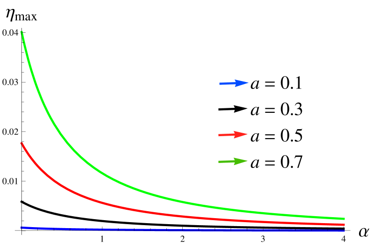
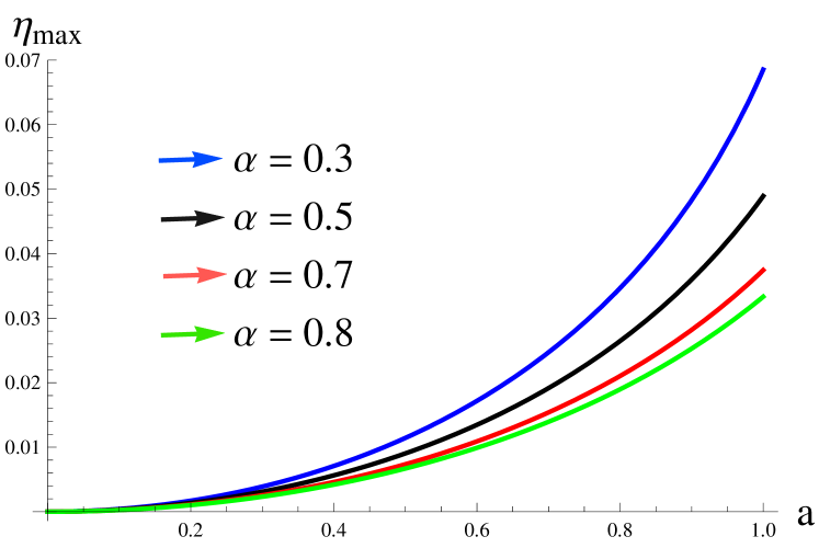
Figure 9: Plots of maximum efficiency of energy extraction as a function of $a$ (left) and $\alpha$ (right).

Consequently, Eq.(16) takes the form

$$[a^{2} + r^{2}-\frac{1}{r^{4}}(a^{2}(-2(1+\alpha)r+\alpha\left(1+\alpha\right))(r^{2}+2(1+\alpha)$$

$$\times r-\alpha\left(1+\alpha\right)))]\Omega^{2}-[\frac{1}{r^{4}}(2a(-2\left(1+\alpha\right)r+\alpha(1$$

$$+ \alpha))(2r^{2}-2\left(1+\alpha\right)r+\alpha\left(1+\alpha\right)))]\Omega+\frac{1}{r^{4}}[(r^{2}-2(1$$

$$+ \alpha)r+\alpha\left(1+\alpha\right))(2r^{2}-2\left(1+\alpha\right)r+\alpha\left(1+\alpha\right))]=0.$$

Using the above equation, the angular velocity of incident particle can be written as

$$\Omega_{(0)} = r^{4}[r^{4}(r^{2}+a^{2})-(a^{2}(-2\left(1+\alpha\right)r+\alpha\left(1+\alpha\right))(r^{2}$$

$$+ 2\left(1+\alpha\right)r-\alpha\left(1+\alpha\right)))]^{-1}\frac{1}{r^{4}}[a(-2\left(1+\alpha\right)r+\alpha$$

$$\times \left(1+\alpha\right))(2r^{2}-2\left(1+\alpha\right)r+\alpha\left(1+\alpha\right))]-[\frac{1}{r^{6}}(2r^{2}$$

$$- 2\left(1+\alpha\right)r+\alpha\left(1+\alpha\right))(r^{6}-2\left(1+\alpha\right)r^{5}+a^{2}(r^{4}$$

$$- 8\left(1+\alpha\right)r^{2})+\alpha\left(1+\alpha\right)(r^{4}+8a^{2}\left(1+\alpha\right)r-2a^{2}$$

$$\times \alpha\left(1+\alpha\right)))]^{1/2}.$$

Substituting Eqs.(20) and (21) into (19), we obtain the efficiency of energy extraction in the form

$$\eta=\frac{(\Omega_{(0)}-\Omega_{-})(g_{tt}+\Omega_{+}g_{t\phi})}{(\Omega_{(+)}-\Omega_{-})(g_{tt}+\Omega_{0}g_{t\phi})}-1.$$

In order to find the maximum value of efficiency ($\eta_{max}$), the incident particle must be splitted at the horizon of BH. Therefore, the above equation becomes

$$\eta_{max}=\frac{\sqrt{1+g_{tt}}-1}{2}|_{r=r_{+}}.$$

The values of maximum efficiency of the energy extraction by Penrose process for different values of the spin parameter $a$ as well as parameter $\alpha$ are given in Table 1. It is observed that maximum efficiency can be enhanced as the parameter $a$ increases. The rotation of a BH has strong effects on the efficiency of energy extraction. It is interesting to note that maximum efficiency decreases with the increasing values of $\alpha$. Moreover, more energy can be extracted from BH when BH rotates rapidly. It is worthwhile to mention that energy extraction efficiency for Kerr-MOG BH is low in comparison with the Kerr BH. For $\alpha=0$ and $a=1$, we have the limiting value for extreme Kerr BH, i.e., $20.7\%$ [15]. So, the obtained results are the generalization of Kerr BH. The graphical behavior of maximum efficiency with respect to $\alpha$ (left) and $a$ (right) for different values of $a$ and $\alpha$, respectively, is depicted in Figure 9. It is found that maximum efficiency has decreasing behavior with the increase of $\alpha$ but increases as spin parameter $a$ increases.

Table 1: The maximum efficiency $\eta_{max}$ $(\%)$ of energy extraction from BH by the Penrose process. a=0.2 a=0.4 a=0.6 a=0.8 a=0.9 a=0.99 a=1.0 $\alpha=0.0$ 0.255 1.077 2.705 5.902 9.009 16.196 20.711 $\alpha=0.01$ 0.251 1.060 2.658 5.776 8.768 15.200 17.298 $\alpha=0.02$ 0.247 1.044 2.612 5.655 8.538 14.397 15.98 $\alpha=0.2$ 0.193 0.805 1.970 4.051 5.752 8.135 8.493 $\alpha=0.3$ 0.170 0.709 1.718 3.466 4.829 6.604 6.853 $\alpha=0.4$ 0.152 0.629 1.514 3.009 4.137 5.536 5.724 $\alpha=0.5$ 0.136 0.563 1.347 2.646 3.598 4.742 4.893

4 Concluding Remarks

In this paper, we have investigated the neutral particle motion and energy extraction via Penrose process around Kerr-MOG BH. The circular motion of particles play an important role in the study of accretion disk theory. Circular timelike geodesics are useful to discuss the dynamics of galaxies and planetary motion. Since BHs are basically non-emitting objects so the investigation of null geodesics around them is also of great interest. The photons coming from other sources carry the astrophysical information that reach to the observer from the accretion disk. We have explored the timelike as well as null geodesics. The effective potential approach is used to study the stability of circular photons orbits. It is observed that the presence of parameter $\alpha$ contributes to increase the instability of photons orbits. The motion becomes unstable for increasing values of $\alpha$. The rotation of BHs also effects the stability of photons orbits. We see that the instability of orbits increases with the increase of rotation of a BH. This situation is much different in comparison with the mining braneworld Kerr-Newman spacetimes where the stable circular photon orbit is almost independent of the spin parameter $a$ [24]. We found that circular orbits of photons around Kerr-MOG BH are more unstable in comparison with the Kerr, Schwarzschild, and Schwarzschild-MOG BHs.

We have discussed the effective force acting on photons, which is more attractive for larger values of spin parameter $a$. It is noted that effective force acting on photons increases with the increasing values of $\alpha$ and does not change as the photons move away from the BH. We have also investigated the instability of circular photons orbits through the Lyapunov exponent. It is observed that Lyapunov exponent initially decreases then increases for higher values of $a$ as compared to smaller values but does not change much more as radial distance increases.

We have examined the energy extraction by Penrose process around Kerr-MOG BH. It is interesting to note that negative energy decreases with the increasing values of parameter $\alpha$. It is worthily to mention that negative energy also decreases when a BH rotates rapidly. We have studied the efficiency of energy extraction from BH. We conclude that the maximum efficiency can be enhanced as the parameter $a$ increases. The rotation of a BH has strong effects on the efficiency of energy extraction. More energy can be extracted from a BH when the rotation of a BH increases. Maximum efficiency has decreasing behavior with the increase of $\alpha$. We have compared the efficiency for Kerr-MOG BH with the Kerr BH, the obtained results indicates that efficiency for Kerr-MOG BH is small than that of the Kerr BH.

References

- [1] Capozziello, S. and De Laurentis, M.: Phys. Rept. 509(2011)167.
- [2] Bamba, K., Capozziello, S., Nojiri, S. and Odintsov, S.D.: Astrophys. Space Sci. 342(2012)155.
- [3] Yousaf, Z., Bamba, K. and Bhatti, M.Z.: Phys. Rev. D 93(2016)064059.
- [4] Yousaf, Z., Bamba, K. and Bhatti, M.Z.: Phys. Rev. D 93(2016)124048.
- [5] Moffat, J.W.: J. Cosmol. Astropart. Phys. 03(2006)004.
- [6] Moffat, J.W. and Rahvar, S.: Mon. Not. R. Astron. Soc. 436(2013)1439.
- [7] Pérez, D., Armengol F.G.L., and Romero G.E.: Phys. Rev. D 95(2017)104047.
- [8] Moffat, J.W.: Inter. J. Mod. Phy. D 16(2007)2075.
- [9] Moffat, J.W. and Rahvar, S.: Mon. Not. R. Astron. Soc. 441(2014)3724.
- [10] Moffat, J.W.: Eur. Phys. J. C 75(2015)130.
- [11] Mureika, J.R., Moffat, J.W. and Faizal, M.: Phys. Lett. B 757(2016)528.
- [12] Lee, H.C. and Han, Y.J.: Eur. Phys. J. C 77(2017)655.
- [13] Sharif, M. and Shahzadi, M.: Eur. Phys. J. C 77(2017)363; J. Exp. Theor. Phys. 127(2018)575.
- [14] Rahvar, S. and Moffat, J.W.: Mon. Not. R. Astron. Soc. 482(2019)4514.
- [15] Chandrasekhar, S.: The Mathematical Theory of Black Holes (Oxford University Press, 1983).
- [16] Bardeen, J.M.: Astrophs. J. 178(1972)347.
- [17] Pugliese, D. and Quevedo, H.: Eur. Phys. J. C 75(2015)130.
- [18] Frolov, V. and Stojkovic, D.: Phys. Rev. D 68(2003)064011.
- [19] Konoplya, R.A.: Phys. Rev. D 74(2006)124015.
- [20] Fernando, S.: Gen. Relativ. Gravit. 44(2012)1857.
- [21] Khoo, F.S. and Ong, Y.C.: Class. Quantum Gravt. 33(2016)235002.
- [22] Pradhan, P.: Universe 4(2018)55.
- [23] Yousaf, Z. and Bhatti, M. Z.: Eur. Phys. J. C 76(2016)267; Bhatti, M. Z. and Yousaf, Z.: Eur. Phys. J. C 76(2016)219; Ann. Phys. 387(2017)253; Int. J. Geom. Meth. Mod. Phys. 15(2018)1850160; Yousaf, Z.: Astrophys. Space Sci. 363(2018)226.
- [24] Stuchlík, Z., Blaschke, M. and Schee, J.: Phys. Rev. D 96(2017)104050.
- [25] Penrose, R.: Nuovo Cimento 1(1969)252; Penrose, R. and Floyd, R. M.: Nature 229(1971)177.
- [26] Nozawa, M. and Maeda, K.I.: Phys. Rev. D 71(2005)084028.
- [27] Pradhan, P.: Class. Quantum Gravt. 32(2015)165001.
- [28] Mukherjee, S.: Phys. Lett. B 778(2018)54.
- [29] Bhat, M., Dhurandhar, S. and Dadhich, N.: J. Astrophys. Astr. 6(1985)85.
- [30] Liu, C.; Chen, S. and Jing, J.: Astrophs. J. 751(2012)148.
- [31] Toshmatov, B. et al.: Astrophys. Space Sci. 357(2015)41.
- [32] Liu, Y. and Liu, W.B.: Phys. Rev. D 97(2018)064024.
- [33] Moffat, J.W.: Eur. Phys. J. C 75(2015)175.
- [34] Abdujabbarov, A., Ahmedov, B. and Hakimov, A.: Phys. Rev. D 83(2011)044053; Toshmatov, B. et al.: Astrophys. Space Sci. 357(2015)41.
- [35] Cardoso, V. et al.: Phys. Rev. D 79(2009)064016.