Exponential energy-preserving methods for charged-particle dynamics in a strong and constant magnetic field

Abstract

In this paper, exponential energy-preserving methods are formulated and analysed for solving charged-particle dynamics in a strong and constant magnetic field. The resulting method can exactly preserve the energy of the dynamics. Moreover, it is shown that the magnetic moment of the considered system is nearly conserved over a long time along this exponential energy-preserving method, which is proved by using modulated Fourier expansions. Other properties of the method including symmetry and convergence are also studied. An illustrated numerical experiment is carried out to demonstrate the long-time behaviour of the method.

Keywords: charged-particle dynamics, exponential energy-preserving methods, modulated Fourier expansions, long-time conservation, strong and constant magnetic field

MSC: 65L06, 65P10, 78A35, 78M25.

1 Introduction

In this paper, we derive and analyse energy-preserving methods for charged-particle dynamics in a strong and constant magnetic field

$$\begin{array}[c]{ll}\ddot{x}=\dot{x}\times\frac{1}{\epsilon}B+F(x),\quad x(t_{0})=x_{0},\quad\dot{x}(t_{0})=\dot{x}_{0},\ \ t\in[t_{0},T],\end{array}$$ (1)

where $x(t)\in{\mathbb{R}}^{3}$ describes the position of a particle, $B=\nabla_{x}\times A(x)$ is a constant magnetic field with the vector potential $A(x)=-\frac{1}{2}x\times B\in{\mathbb{R}}^{3}$ and $F(x)=-\nabla_{x}U(x)$ is an electric field with the scalar potential $U(x)$. Following [15], we are devoted to the situation of a small positive acaling parameter $0<\epsilon\ll 1$ and assume that $\left|B\right|\geq 1$ in the Euclidean norm. The energy of this dynamics is given by

$$E(x,v)=\frac{1}{2}\left|v\right|^{2}+U(x),$$ (2)

where $v=\dot{x}$ is the velocity of the particle. Denote the constant vector $B$ by $B=(B_{1},B_{2},B_{3})^{\intercal}$ with $B_{i}\in{\mathbb{R}}$ for $i=1,2,3.$ By the definition of the cross product, we obtain $\dot{x}\times B=\tilde{B}\dot{x},$ where $\tilde{B}$ is a skew symmetric matrix

$$\tilde{B}=\left(\begin{array}[]{ccc}0&B_{3}&-B_{2}\\ -B_{3}&0&B_{1}\\ B_{2}&-B_{1}&0\\ \end{array}\right).$$

The system (1) as well as $v=\dot{x}$ can be rewritten as

$$\begin{array}[c]{ll}\dot{x}=v,\ \dot{v}=\frac{1}{\epsilon}\tilde{B}v+F(x).\end{array}$$ (3)

With the analysis given in [1, 4], it is well known that the magnetic moment

$$I(x,v)=\frac{\left|v_{\perp}\right|^{2}}{2\left|B\right|}=\frac{1}{2\left|\tilde{B}\right|^{3}}\left|\tilde{B}v\right|^{2}$$ (4)

is an adiabatic invariant, where $v_{\perp}=\frac{v\times B}{\left|B\right|}$ is orthogonal to $B$ and $|\tilde{B}|=\sqrt{B_{1}^{2}+B_{2}^{2}+B_{3}^{2}}.$ Recently, it has been shown in [15] that this quantity is nearly conserved over long time scales, which is proved by using the technique of modulated Fourier expansion with state-dependent frequencies and eigenvectors.

Charged-particle dynamics have been received much attention for a long time (see, e.g. [1, 4]) and many effective methods have been developed for solving this system. The Boris method was presented in [2] and it was researched further in [8, 13, 26]. Various other kinds of methods have also been researched for charged-particle dynamics, such as volume-preserving algorithms in [17], symplectic or K-symplectic algorithms in [18, 29, 33, 35], and symmetric multistep methods in [14]. It is worth mentioning that, more recently, a variational integrator has been studied in [15] for solving charged-particle dynamics in a strong magnetic field. In this paper we are interested in the formulation and analysis of energy-preserving (EP) methods when applied to charged-particle dynamics in a strong and constant magnetic field.

For the energy-preserving methods, there have been a lot of studies on this topic. Many different EP methods have been presented and analysed, such as the average vector field (AVF) method (see, e.g. [5, 27]), discrete gradient methods (see, e.g. [23]), Hamiltonian Boundary Value Methods (see, e.g. [3]), EP collocation methods (see, e.g. [10]) and trigonometric/exponential EP methods (see, e.g. [21, 31, 34]). Based on these work, we will derive and analyse novel EP integrators for charged-particle dynamics in a strong and constant magnetic field. The long time magnetic moment conservation of the new integrator will also be researched via its modulated Fourier expansion. The technique of modulated Fourier expansion was firstly given in [11] and then it has been successfully used in the study of long-time behaviour for numerical methods/differential equations (see, e.g. [6, 7, 9, 12, 16, 28]).

The rest of this paper is organized as follows. In Section 2, we first formulate the scheme of the method and then prove that it is symmetric. In Section 3, two main results concerning energy preservation and magnetic moment preservation are presented and a numerical experiment is reported to support these results. The proofs of the two main results are given in Sections 4-5, respectively. The concluding remarks of this paper are given in the last section.

2 Formulation of the method

In order to effectively solve the system (3), we consider the following method.

Definition 2.1

The exponential energy-preserving method for solving (3) is defined by:

$$\left\{\begin{array}[c]{ll}x_{n+1}=x_{n}+h\varphi_{1}(\frac{h}{\epsilon}\tilde{B})v_{n}+h^{2}\varphi_{2}(\frac{h}{\epsilon}\tilde{B})\int_{0}^{1}F\big{(}x_{n}+\sigma(x_{n+1}-x_{n})\big{)}d\sigma,\\ v_{n+1}=e^{\frac{h}{\epsilon}\tilde{B}}v_{n}+h\varphi_{1}(\frac{h}{\epsilon}\tilde{B})\int_{0}^{1}F\big{(}x_{n}+\sigma(x_{n+1}-x_{n})\big{)}d\sigma,\end{array}\right.$$ (5)

where $h$ is a stepsize and the $\varphi$-functions are defined by

$$\varphi_{0}(z)=e^{z},\ \ \varphi_{k}(z)=\int_{0}^{1}e^{(1-\sigma)z}\frac{\sigma^{k-1}}{(k-1)!}d\sigma,\ \ k=1,2.$$ (6)

We denote this method by EEP.

Remark 2.2

It is noted that this kind of method belongs to exponential integrators, which have been widely developed and researched for solving highly oscillatory systems (see, e.g. [19, 20, 21, 24, 30, 32]).

Proposition 2.3

The EEP integrator (5) is symmetric.

Proof Exchanging $(x_{n},v_{n})\leftrightarrow(x_{n+1},v_{n+1})$ and $h\leftrightarrow-h$ in (5) yields

$$\left\{\begin{array}[c]{ll}x_{n}=x_{n+1}-h\varphi_{1}(-\frac{h}{\epsilon}\tilde{B})v_{n+1}+h^{2}\varphi_{2}(-\frac{h}{\epsilon}\tilde{B})\int_{0}^{1}F\big{(}x_{n}+\sigma(x_{n+1}-x_{n})\big{)}d\sigma,\\ v_{n}=e^{-\frac{h}{\epsilon}\tilde{B}}v_{n+1}-h\varphi_{1}(-\frac{h}{\epsilon}\tilde{B})\int_{0}^{1}F\big{(}x_{n}+\sigma(x_{n+1}-x_{n})\big{)}d\sigma,\end{array}\right.$$ (7)

where the following fact has been used

$$\int_{0}^{1}F\big{(}x_{n+1}+\sigma(x_{n}-x_{n+1})\big{)}d\sigma=\int_{0}^{1}F\big{(}x_{n}+\sigma(x_{n+1}-x_{n})\big{)}d\sigma.$$

We thus obtain

$$v_{n+1}=e^{\frac{h}{\epsilon}\tilde{B}}v_{n}+he^{\frac{h}{\epsilon}\tilde{B}}\varphi_{1}(-\frac{h}{\epsilon}\tilde{B})\mathcal{I}=e^{\frac{h}{\epsilon}\tilde{B}}v_{n}+h\varphi_{1}(\frac{h}{\epsilon}\tilde{B})\mathcal{I}$$

by considering the second formula of (7). Inserting this into the first formula of (7), we get

$$\begin{array}[]{rl}x_{n+1}&=x_{n}+h\varphi_{1}(-\frac{h}{\epsilon}\tilde{B})v_{n+1}-h^{2}\varphi_{2}(-\frac{h}{\epsilon}\tilde{B})\mathcal{I}\\ &=x_{n}+h\varphi_{1}(-\frac{h}{\epsilon}\tilde{B})e^{\frac{h}{\epsilon}\tilde{B}}v_{n}+h^{2}\big{(}\varphi_{1}(-\frac{h}{\epsilon}\tilde{B})\varphi_{1}(\frac{h}{\epsilon}\tilde{B})-\varphi_{2}(-\frac{h}{\epsilon}\tilde{B})\big{)}\mathcal{I}\\ &=x_{n}+h\varphi_{1}(\frac{h}{\epsilon}\tilde{B})v_{n}+h^{2}\varphi_{2}(\frac{h}{\epsilon}\tilde{B})\mathcal{I}.\end{array}$$

Therefore, the energy-preserving integrator (5) is symmetric.

3 Main results and numerical experiment

3.1 Main results

Before presenting the main results of this paper, we need the following assumptions, which have been considered in [11, 16].

Assumption 3.1

• We consider the initial values

  $$x_{0}=\mathcal{O}(1),\ \ \ v_{0}=\mathcal{O}(1)$$

  such that the energy $E$ is bounded independently of $\epsilon$ along the solution.

• It is assumed that the numerical solution stays in a compact set.

• We require a lower bound on the stepsize $h\tilde{\omega}\geq c_{0}>0$ with $\tilde{\omega}=\frac{|\tilde{B}|}{\epsilon}$.

• The following numerical non-resonance condition is assumed to be true

  $$|\sin(\frac{1}{2}kh\tilde{\omega})|\geq c\sqrt{h}\ \ \mathrm{for}\ \ k=1,2,\ldots,N\ \ \mathrm{with}\ \ N\geq 2,$$ (8)

  which imposes a restriction on $N$ for a given $h$ and $\tilde{\omega}$.

We first give the result about the energy preservation of the EEP method.

Theorem 3.2

(Energy preservation.) The EEP integrator (5) preserves the energy $E$ in (2) exactly, i.e.,

$$E(x_{n+1},v_{n+1})=E(x_{n},v_{n})\qquad\textmd{for}\qquad n=0,1,\ldots.$$

Now, we present the result about the long time magnetic moment conservation of the EEP method.

Theorem 3.3

(Magnetic moment conservation.) Under the conditions of Assumption 3.1, the long time magnetic moment is nearly conserved over long times by the EEP method

$$I(x_{n},v_{n})=I(x_{0},v_{0})+\mathcal{O}\Big{(}\frac{1}{\left|\cos(\frac{1}{2}h\tilde{\omega})\right|}h\Big{)}+\mathcal{O}(h),$$

where $0\leq nh\leq h^{-N+1}.$ The constants symbolized by $\mathcal{O}$ depend on $N$, the final time $T$ and the constants in the assumptions, but are independent of $n,\ h,\ \epsilon$.

Remark 3.4

We note that it is easy to make a choice of the stepsize $h$ such that $\left|\cos(\frac{1}{2}h\tilde{\omega})\right|$ is not small. In this case, an improved result concerning the long time magnetic moment conservation is obtained

$$I(x_{n},v_{n})=I(x_{0},v_{0})+\mathcal{O}(h)$$

for $0\leq nh\leq h^{-N+1}.$

3.2 Numerical experiment

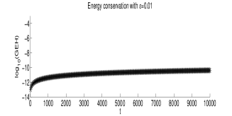
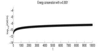
Figure 1: the logarithm of the energy relative errors against $t$.

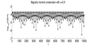
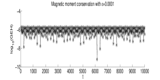
Figure 2: the logarithm of the magnetic moment relative errors against $t$.

As an illustrative numerical experiment, we consider the charged particle system of [14] with a constant magnetic field and an additional factor $1/\epsilon$. The system can be given by (1) with the potential $U(x)=\frac{1}{100\sqrt{x_{1}^{2}+x_{2}^{2}}}$ and the constant magnetic field $B=(0,0,1)^{\intercal}.$ The initial values are chosen as $x(0)=(0.7,1,0.1)^{\intercal}$ and $v(0)=(0.9,0.5,0.4)^{\intercal}.$

We consider applying four-point Gauss-Legendre’s rule to the integral of the EEP integrator (5). The fixed-point iteration is chosen here and we set $10^{-16}$ as the error tolerance and $50$ as the maximum number of each iteration. We choose $\epsilon=0.01,0.0001$. This problem is integrated on $[0,10000]$ with $h=0.01$ and see Figures 1-2 for the relative errors $(H(x_{n},v_{n})-H(x^{0},v^{0}))/H(x^{0},v^{0})$ of the energy and $(I(x_{n},v_{n})-I(x^{0},v^{0}))/I(x^{0},v^{0})$ of the magnetic moment, respectively. In order to show the performance of our EEP method, we choose Boris method for comparison. We consider $\epsilon=0.0001$ and solve this system on $[0,10000]$ with $h=0.01$. The results of Boris method are shown in Figure 3. Finally, the problem is solved with $\epsilon=0.05,$ $T=10,100,1000$ and $h=1/(50\times 2^{i})$ for $i=0,\ldots,3$. The global errors are shown in Figure 4.

From the results, it can be observed that our EEP method shows an excellent energy-preserving property, a prominent long-term behavior in the numerical magnetic moment conservation and a good accuracy. All these observations support the theoretical results given in Theorems 3.2- 3.3.

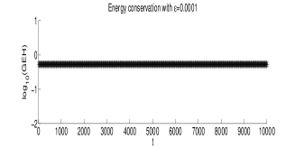
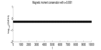
Figure 3: the logarithm of the relative errors for Boris method against $t$.

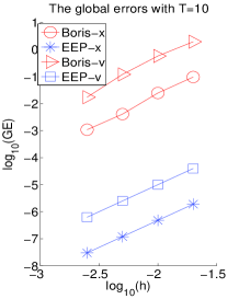
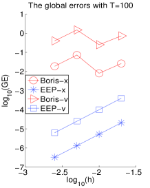
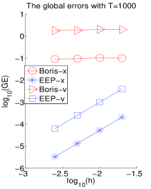
Figure 4: the global errors.

4 Proof of energy preservation

In this section, we give the proof of Theorem 3.2.

Proof  In this paper, we let $\mathcal{I}:=\int_{0}^{1}F\big{(}x_{n}+\sigma(x_{n+1}-x_{n})\big{)}d\sigma$ for brevity. We firstly compute

$$\begin{array}[c]{ll}E(x_{n+1},v_{n+1})=\dfrac{1}{2}v_{n+1}^{\intercal}v_{n+1}+U(x_{n+1}).\end{array}$$ (9)

Keeping the fact in mind that $\tilde{B}$ is skew-symmetric, one obtains that

$$(e^{\frac{h}{\epsilon}\tilde{B}})^{\intercal}=e^{-\frac{h}{\epsilon}\tilde{B}},\ (\varphi_{1}(\frac{h}{\epsilon}\tilde{B}))^{\intercal}=\varphi_{1}(-\frac{h}{\epsilon}\tilde{B}),\ (\varphi_{2}(\frac{h}{\epsilon}\tilde{B}))^{\intercal}=\varphi_{2}(-\frac{h}{\epsilon}\tilde{B}).$$

Inserting the second formula of (5) into (9) with some manipulation yields

$$E(x_{n+1},v_{n+1})=\frac{1}{2}\big{(}e^{\frac{h}{\epsilon}\tilde{B}}v_{n}+h\varphi_{1}(\frac{h}{\epsilon}\tilde{B})\mathcal{I}\big{)}^{\intercal}\big{(}e^{\frac{h}{\epsilon}\tilde{B}}v_{n}+h\varphi_{1}(\frac{h}{\epsilon}\tilde{B})\mathcal{I}\big{)}+U(x_{n+1})$$

$$= \dfrac{1}{2}v_{n}^{\intercal}e^{-\frac{h}{\epsilon}\tilde{B}}e^{\frac{h}{\epsilon}\tilde{B}}v_{n}+h\mathcal{I}^{\intercal}\varphi_{1}(-\frac{h}{\epsilon}\tilde{B})e^{\frac{h}{\epsilon}\tilde{B}}v_{n}+\dfrac{1}{2}h^{2}\mathcal{I}^{\intercal}\varphi_{1}(-\frac{h}{\epsilon}\tilde{B})\varphi_{1}(\frac{h}{\epsilon}\tilde{B})\mathcal{I}+U(x_{n+1}).$$

It follows from (6) that $\varphi_{1}(-\frac{h}{\epsilon}\tilde{B})e^{\frac{h}{\epsilon}\tilde{B}}=\varphi_{1}(\frac{h}{\epsilon}\tilde{B}).$ Therefore, we obtain

$$E(x_{n+1},v_{n+1})=\dfrac{1}{2}v_{n}^{\intercal}v_{n}+h\mathcal{I}^{\intercal}\varphi_{1}(\frac{h}{\epsilon}\tilde{B})v_{n}+\dfrac{1}{2}h^{2}\mathcal{I}^{\intercal}\varphi_{1}(-\frac{h}{\epsilon}\tilde{B})\varphi_{1}(\frac{h}{\epsilon}\tilde{B})\mathcal{I}+U(x_{n+1}).$$ (10)

On the other hand, it can be checked that

$$U(x_{n})-U(x_{n+1})=-\int_{0}^{1}dU((1-\tau)x_{n}+\tau x_{n+1})$$

$$= -\int_{0}^{1}(x_{n+1}-x_{n})^{\intercal}\nabla_{x}U((1-\tau)x_{n}+\tau x_{n+1})d\tau=\mathcal{I}^{\intercal}(x_{n+1}-x_{n})$$

$$= h\mathcal{I}^{\intercal}\varphi_{1}(\frac{h}{\epsilon}\tilde{B})v_{n}+h^{2}\mathcal{I}^{\intercal}\varphi_{2}(\frac{h}{\epsilon}\tilde{B})\mathcal{I},$$

where the first equation of (5) has been used. Inserting this result into (10) implies

$$E(x_{n+1},v_{n+1})= \dfrac{1}{2}v_{n}^{\intercal}v_{n}+h\mathcal{I}^{\intercal}\varphi_{1}(\frac{h}{\epsilon}\tilde{B})v_{n}+\dfrac{1}{2}h^{2}\mathcal{I}^{\intercal}\varphi_{1}(-\frac{h}{\epsilon}\tilde{B})\varphi_{1}(\frac{h}{\epsilon}\tilde{B})\mathcal{I}+U(x_{n})$$ (11)

$$-h\mathcal{I}^{\intercal}\varphi_{1}(\frac{h}{\epsilon}\tilde{B})v_{n}-h^{2}\mathcal{I}^{\intercal}\varphi_{2}(\frac{h}{\epsilon}\tilde{B})\mathcal{I}$$

$$= \dfrac{1}{2}v_{n}^{\intercal}v_{n}+U(x_{n})+\dfrac{1}{2}h^{2}\mathcal{I}^{\intercal}\Big{(}\varphi_{1}(-\frac{h}{\epsilon}\tilde{B})\varphi_{1}(\frac{h}{\epsilon}\tilde{B})-2\varphi_{2}(\frac{h}{\epsilon}\tilde{B})\Big{)}\mathcal{I}.$$

It follows from the definition (6) that $\varphi_{1}(-\frac{h}{\epsilon}\tilde{B})\varphi_{1}(\frac{h}{\epsilon}\tilde{B})-2\varphi_{2}(\frac{h}{\epsilon}\tilde{B})=\sum\limits_{k=1}^{\infty}c_{k}\big{(}\frac{h}{\epsilon}\tilde{B}\big{)}^{2k+1}$ with the coefficients $c_{k}$ for $k=1,2,\ldots$, which gives that

$$\Big{(}\varphi_{1}(-\frac{h}{\epsilon}\tilde{B})\varphi_{1}(\frac{h}{\epsilon}\tilde{B})-2\varphi_{2}(\frac{h}{\epsilon}\tilde{B})\Big{)}^{\intercal}=\sum\limits_{k=1}^{\infty}c_{k}\big{(}-\frac{h}{\epsilon}\tilde{B}\big{)}^{2k+1}$$

$$=-\sum\limits_{k=1}^{\infty}c_{k}\big{(}\frac{h}{\epsilon}\tilde{B}\big{)}^{2k+1}=-\Big{(}\varphi_{1}(-\frac{h}{\epsilon}\tilde{B})\varphi_{1}(\frac{h}{\epsilon}\tilde{B})-2\varphi_{2}(\frac{h}{\epsilon}\tilde{B})\Big{)}.$$

Based on this result, one arrives at

$$\mathcal{I}^{\intercal}\Big{(}\varphi_{1}(-\frac{h}{\epsilon}\tilde{B})\varphi_{1}(\frac{h}{\epsilon}\tilde{B})-2\varphi_{2}(\frac{h}{\epsilon}\tilde{B})\Big{)}\mathcal{I} =\Big{[}\mathcal{I}^{\intercal}\Big{(}\varphi_{1}(-\frac{h}{\epsilon}\tilde{B})\varphi_{1}(\frac{h}{\epsilon}\tilde{B})-2\varphi_{2}(\frac{h}{\epsilon}\tilde{B})\Big{)}\mathcal{I}\Big{]}^{\intercal}$$

$$=-\mathcal{I}^{\intercal}\Big{(}\varphi_{1}(-\frac{h}{\epsilon}\tilde{B})\varphi_{1}(\frac{h}{\epsilon}\tilde{B})-2\varphi_{2}(\frac{h}{\epsilon}\tilde{B})\Big{)}\mathcal{I},$$

which shows that $\mathcal{I}^{\intercal}\Big{(}\varphi_{1}(-\frac{h}{\epsilon}\tilde{B})\varphi_{1}(\frac{h}{\epsilon}\tilde{B})-2\varphi_{2}(\frac{h}{\epsilon}\tilde{B})\Big{)}\mathcal{I}=0.$ Therefore, (11) becomes

$$E(x_{n+1},v_{n+1})=\dfrac{1}{2}v_{n}^{\intercal}v_{n}+U(x_{n})=E(x_{n},v_{n}).$$

5 Proof of the magnetic moment conservation

This section is devoted to the proof of Theorem 3.3. Modulated Fourier expansion will be used here. We will first derive the modulated Fourier expansion for the EEP method in Subsection 5.1 and then show an almost-invariant of the expansion in Subsection 5.2. Based on these analysis, Theorem 3.3 will be proved immediately.

Since the matrix $\tilde{B}$ is skew-symmetric, there exists a unitary matrix $P$ and a diagonal matrix $\Lambda$ such that $\tilde{B}=P\Lambda P^{\textup{H}}$ with $\Lambda=\textmd{diag}(-|\tilde{B}|\mathrm{i},0,|\tilde{B}|\mathrm{i})$. By the linear change of variable

$$\tilde{x}(t)=P^{\textup{H}}x(t),\quad\tilde{v}(t)=P^{\textup{H}}v(t),$$ (12)

we rewrite the system (3) as

$$\begin{array}[c]{ll}\dot{\tilde{x}}=\tilde{v},&\tilde{x}_{0}=P^{\textup{H}}x_{0},\\ \dot{\tilde{v}}=\mathrm{i}\tilde{\Omega}\tilde{v}+\tilde{F}(\tilde{x}),&\tilde{v}_{0}=P^{\textup{H}}v_{0},\end{array}$$ (13)

where $\tilde{\Omega}=\textmd{diag}(-\tilde{\omega},0,\tilde{\omega})$ with $\tilde{\omega}=\frac{|\tilde{B}|}{\epsilon}$ and $\tilde{F}(\tilde{x})=P^{\textup{H}}F(P\tilde{x})=-\nabla_{\tilde{x}}U(P\tilde{x})$. In this paper, a vector $x$ in ${\mathbb{R}}^{3}$ or ${\mathbb{C}}^{3}$ is denoted by $x=(x_{-1},x_{0},x_{1})^{\intercal}$. For the transformed system (13), its magnetic moment has the following form

$$\begin{array}[c]{ll}I(x,v)&=\frac{1}{2\left|\tilde{B}\right|^{3}}\left|\tilde{B}v\right|^{2}=\frac{1}{2\left|\tilde{B}\right|^{3}}\left|P\Lambda\tilde{v}\right|^{2}=\frac{1}{2\left|\tilde{B}\right|^{3}}\left|\Lambda\tilde{v}\right|^{2}\\ &=\frac{1}{2\left|\tilde{B}\right|^{3}}\left|\tilde{B}\right|^{2}(\left|\tilde{v}_{-1}\right|^{2}+\left|\tilde{v}_{1}\right|^{2})=\frac{1}{2\left|\tilde{B}\right|}(\left|\tilde{v}_{-1}\right|^{2}+\left|\tilde{v}_{1}\right|^{2}):=\tilde{I}(\tilde{x},\tilde{v}).\end{array}$$ (14)

The EEP integrator (5) for solving this transformed system is defined as

$$\left\{\begin{array}[c]{ll}&\tilde{x}_{n+1}=\tilde{x}_{n}+h\varphi_{1}(\mathrm{i}h\tilde{\Omega})\tilde{v}_{n}+h^{2}\varphi_{2}(\mathrm{i}h\tilde{\Omega})\int_{0}^{1}\tilde{F}\big{(}\tilde{x}_{n}+\sigma(\tilde{x}_{n+1}-\tilde{x}_{n})\big{)}d\sigma,\\ &\tilde{v}_{n+1}=e^{\mathrm{i}h\tilde{\Omega}}\tilde{v}_{n}+h\varphi_{1}(\mathrm{i}h\tilde{\Omega})\int_{0}^{1}\tilde{F}\big{(}\tilde{x}_{n}+\sigma(\tilde{x}_{n+1}-\tilde{x}_{n})\big{)}d\sigma.\end{array}\right.$$ (15)

In this section, the following five operators will be used:

$$L_{1}(hD): =\mathrm{e}^{hD}-e^{\mathrm{i}h\tilde{\Omega}},$$ (16)

$$L_{2}(hD): =\varphi_{1}(\mathrm{i}h\tilde{\Omega})\mathrm{e}^{\frac{1}{2}hD},$$

$$L_{3}(hD): =\varphi_{1}(\mathrm{i}h\tilde{\Omega})(\mathrm{e}^{hD}-1),$$

$$L_{4}(hD): =h\varphi_{2}(\mathrm{i}h\tilde{\Omega})\mathrm{e}^{hD}+h\varphi^{2}_{1}(\mathrm{i}h\tilde{\Omega})-he^{\mathrm{i}h\tilde{\Omega}}\varphi_{2}(\mathrm{i}h\tilde{\Omega}),$$

$$L_{5}(hD,\tau,k): =(1-\tau)\mathrm{e}^{-\mathrm{i}\frac{h}{2}k\tilde{\omega}}\mathrm{e}^{-\frac{h}{2}D}+\tau\mathrm{e}^{\mathrm{i}\frac{h}{2}k\tilde{\omega}}\mathrm{e}^{\frac{h}{2}D},$$

$$L(hD): =(L_{1}L_{2}^{-1}L_{3}L_{4}^{-1})(hD),$$

where $D$ is the differential operator (see [16]). We have the following properties of these operators.

Proposition 5.1

The Taylor expansions of the operator $L(hD)$ are expressed by

$$L(hD)=-\mathrm{i}\tilde{\Omega}hD+hD^{2}+\cdots,$$

$$L(hD+\mathrm{i}h\tilde{\omega})=\textmd{diag}\Big{(}-\frac{h\tilde{\omega}^{2}\sin(h\tilde{\omega})}{h\tilde{\omega}\cos(\frac{h\tilde{\omega}}{2})-\sin(\frac{h\tilde{\omega}}{2})},\frac{-8\csc(h\tilde{\omega})\sin^{3}(\frac{h\tilde{\omega}}{2})}{h},0\Big{)}+\textmd{diag}$$

$$\Big{(}\frac{h^{2}\tilde{\omega}^{2}(4h\tilde{\omega}\cos^{3}(\frac{h\tilde{\omega}}{2})+\sin(\frac{h\tilde{\omega}}{2})-\sin(\frac{3h\tilde{\omega}}{2}))}{4(\sin(\frac{h\tilde{\omega}}{2})-h\tilde{\omega}\cos(\frac{h\tilde{\omega}}{2}))^{2}},(3+\cos(h\tilde{\omega}))\sec(\frac{3h\tilde{\omega}}{2})\tan(\frac{3h\tilde{\omega}}{2}),\frac{1}{2}h^{2}\tilde{\omega}^{2}\csc(\frac{h\tilde{\omega}}{2})\Big{)}(\mathrm{i}D)+\cdots,$$

$$L(hD-\mathrm{i}h\tilde{\omega})=\textmd{diag}\Big{(}0,\frac{-8\csc(h\tilde{\omega})\sin^{3}(\frac{h\tilde{\omega}}{2})}{h},-\frac{h\tilde{\omega}^{2}\sin(h\tilde{\omega})}{h\tilde{\omega}\cos(\frac{h\tilde{\omega}}{2})-\sin(\frac{h\tilde{\omega}}{2})}\Big{)}+\textmd{diag}$$

$$\Big{(}-\frac{1}{2}h^{2}\tilde{\omega}^{2}\csc(\frac{h\tilde{\omega}}{2}),-(3+\cos(h\tilde{\omega}))\sec(\frac{3h\tilde{\omega}}{2})\tan(\frac{3h\tilde{\omega}}{2}),\frac{h^{2}\tilde{\omega}^{2}(4h\tilde{\omega}\cos^{3}(\frac{h\tilde{\omega}}{2})+\sin(\frac{h\tilde{\omega}}{2})-\sin(\frac{3h\tilde{\omega}}{2}))}{-4(\sin(\frac{h\tilde{\omega}}{2})-h\tilde{\omega}\cos(\frac{h\tilde{\omega}}{2}))^{2}}\Big{)}(\mathrm{i}D)+\cdots,$$

$$L(hD+\mathrm{i}kh\tilde{\omega})=-8h\tilde{\Omega}^{2}\sin(\frac{hk\omega I}{2})\sin(\frac{-h\tilde{\Omega}+hk\omega I}{2})\Gamma_{1}/\Gamma_{2}+(\cdot)(\mathrm{i}D)+\cdots,\ \textmd{for}\ \left|k\right|>1,$$

where

$$\Gamma_{1}= \cos(\frac{h\tilde{\Omega}-hk\omega I}{2})-\cos(\frac{h\tilde{\Omega}+hk\omega I}{2})+h\tilde{\Omega}\sin(\frac{h\tilde{\Omega}-hk\omega I}{2}),$$

$$\Gamma_{2}= \big{(}-I+\cos(h\tilde{\Omega})+\cos(hk\tilde{\omega})I-\cos(h\tilde{\Omega}+hk\tilde{\omega}I)+h\tilde{\Omega}\sin(h\tilde{\Omega})-h\tilde{\Omega}\sin(hk\tilde{\omega})I\big{)}^{2}$$

$$+\big{(}-h\tilde{\Omega}\cos(h\tilde{\Omega})+h\tilde{\Omega}\cos(hk\tilde{\omega})I+\sin(h\tilde{\Omega})+\sin(hk\tilde{\omega})I-\sin(h\tilde{\Omega}+hk\tilde{\omega}I)\big{)}^{2}.$$

The operator $(L_{3}L_{4}^{-1})(hD)$ has the following Taylor expansions

$$(L_{3}L_{4}^{-1})(hD)=D-\frac{-2+h\tilde{\Omega}\cot(\frac{h\tilde{\Omega}}{2})}{2h\tilde{\Omega}}(\mathrm{i}hD^{2})+\cdots,$$

$$(L_{3}L_{4}^{-1})(hD-\mathrm{i}h\tilde{\omega})=\mathrm{i}\textmd{diag}\Big{(}-\tilde{\omega},-\frac{2\tan(\frac{h\tilde{\omega}}{2})}{h},\frac{\tilde{\omega}}{-1+h\tilde{\omega}\cot(\frac{h\tilde{\omega}}{2})}\Big{)}+\cdots,$$

$$(L_{3}L_{4}^{-1})(hD+\mathrm{i}h\tilde{\omega})=\mathrm{i}\textmd{diag}\Big{(}\frac{\tilde{\omega}}{-1+h\tilde{\omega}\cot(\frac{h\tilde{\omega}}{2})},\frac{2\tan(\frac{h\tilde{\omega}}{2})}{h},\tilde{\omega}\Big{)}+\cdots,$$

$$(L_{3}L_{4}^{-1})(hD+\mathrm{i}hk\tilde{\omega})=-8\tilde{\Omega}\sin(\frac{h\Omega}{2})\sin(\frac{hk\omega I}{2})\Gamma_{1}/\Gamma_{2}\mathrm{i}+(\cdot)(D)+\cdots,\ \textmd{for}\ \left|k\right|>1.$$

Moreover, for the operator $L_{5}(hD,\tau,k)$ and $\left|k\right|>0$, it is true that

$$L_{5}(hD,\frac{1}{2},k)=\cos(\frac{kh\tilde{\omega}}{2})+\frac{1}{2}\sin(\frac{kh\tilde{\omega}}{2})(\textmd{i}hD)+\cdots.$$

5.1 Modulated Fourier expansion

A modulated Fourier expansion of the EEP method (15) for solving the transformed system (13) is given as follows.

Theorem 5.2

Assume that all the conditions of Assumption 3.1 hold. The numerical solution given by the EEP integrator (15) admits a modulated Fourier expansion

$$\tilde{x}_{n}=\sum\limits_{|k|<N}\mathrm{e}^{\mathrm{i}k\tilde{\omega}t}\tilde{\zeta}^{k}(t)+\tilde{R}_{h,N}(t),\ \ \tilde{v}_{n}=\sum\limits_{|k|<N}\mathrm{e}^{\mathrm{i}k\tilde{\omega}t}\tilde{\eta}^{k}(t)+\tilde{S}_{h,N}(t),$$ (17)

where $0\leq t=nh\leq T$, $N$ is a fixed integer such that (8) holds and the remainder terms are bounded by

$$\tilde{R}_{h,N}(t)=\mathcal{O}(t^{2}h^{N}),\ \ \ \ \tilde{S}_{h,N}(t)=\mathcal{O}(t^{2}h^{N-1}).\\$$ (18)

The bounds of the coefficient functions of $\tilde{\zeta}^{k}$ as well as all their derivatives are given by

$$\dot{\tilde{\zeta}}^{0}_{\pm 1}=\mathcal{O}(\epsilon),\qquad\quad\ \ddot{\tilde{\zeta}}^{0}_{0}=\mathcal{O}(1),\quad\qquad\ \ \dot{\tilde{\zeta}}^{1}_{1}=\mathcal{O}(\epsilon),\quad\ \ \quad\ \ \ \dot{\tilde{\zeta}}^{-1}_{-1}=\mathcal{O}(\epsilon),$$ (19)

$$\tilde{\zeta}^{1}_{-1}=\mathcal{O}\big{(}\frac{\epsilon^{3}}{\sqrt{h}}\big{)}\qquad\ \tilde{\zeta}^{1}_{0}=\mathcal{O}(\epsilon^{2}),\qquad\ \ \ \ \ \tilde{\zeta}^{-1}_{1}=\mathcal{O}(\frac{\epsilon^{3}}{\sqrt{h}}),\quad\ \ \ \tilde{\zeta}^{-1}_{0}=\mathcal{O}(\epsilon^{2}),$$

$$\tilde{\zeta}^{k}=\mathcal{O}(\epsilon^{\left|k\right|+1})\quad\ \ \ \ \textmd{for}\ \left|k\right|>1,$$

and further by

$$\tilde{\zeta}^{0}_{\pm 1}=\mathcal{O}(1),\qquad\quad\tilde{\zeta}^{0}_{0}=\mathcal{O}(1),\quad\qquad\tilde{\zeta}^{1}_{1}=\mathcal{O}(\epsilon),\quad\ \ \ \ \tilde{\zeta}^{-1}_{-1}=\mathcal{O}(\epsilon).$$ (20)

The bounds of the coefficient functions of $\tilde{\eta}^{k}$ as well as all their derivatives are

$$\tilde{\eta}^{0}_{\pm 1}=\mathcal{O}(\epsilon),\qquad\qquad\quad\ \ \tilde{\eta}^{0}_{0}=\mathcal{O}(1),\quad\qquad\ \ \ \tilde{\eta}^{1}_{1}=\mathrm{i}\tilde{w}\tilde{\zeta}_{1}^{1}(t)+\mathcal{O}(\epsilon),\quad\ \ \ \tilde{\eta}^{-1}_{-1}=\mathrm{i}\tilde{w}\tilde{\zeta}_{-1}^{-1}(t)+\mathcal{O}(\epsilon),$$ (21)

$$\tilde{\eta}^{1}_{-1}=\mathcal{O}\big{(}\frac{\epsilon^{3}}{\sqrt{h}\left|\cos(\frac{h\tilde{\omega}}{2})\right|}\big{)},\ \ \tilde{\eta}^{1}_{0}=\mathcal{O}\big{(}\frac{\epsilon^{2}}{\left|\cos(\frac{h\tilde{\omega}}{2})\right|}\big{)},\ \ \tilde{\eta}^{-1}_{1}=\mathcal{O}\big{(}\frac{\epsilon^{3}}{\sqrt{h}\left|\cos(\frac{h\tilde{\omega}}{2})\right|}\big{)},\ \ \tilde{\eta}^{-1}_{0}=\mathcal{O}\big{(}\frac{\epsilon^{2}}{\left|\cos(\frac{h\tilde{\omega}}{2})\right|}\big{)},$$

$$\tilde{\eta}^{k}=\mathcal{O}(\epsilon^{\left|k\right|})\qquad\qquad\qquad\textmd{for}\ \left|k\right|>1,$$

By noticing $P\tilde{\zeta}^{-k}=\bar{P}\overline{\tilde{\zeta}^{k}},$ $P\tilde{\eta}^{-k}=\bar{P}\overline{\tilde{\eta}^{k}}$ and $P^{\textup{H}}\bar{P}=\left(\begin{array}[]{ccc}0&0&1\\ 0&1&0\\ 1&0&0\\ \end{array}\right),$ one obtains that $\tilde{\zeta}_{-l}^{-k}=\overline{\tilde{\zeta}_{l}^{k}}$ and $\tilde{\eta}_{-l}^{-k}=\overline{\tilde{\eta}_{l}^{k}}$. The constants symbolized by the notation depend on the constants from Assumption 3.1 and the final time $T$, but are independent of $h$ and $\tilde{\omega}$.

Proof  We will construct the functions

$$\tilde{x}_{h}(t)=\sum\limits_{|k|<N}\mathrm{e}^{\mathrm{i}k\tilde{\omega}t}\tilde{\zeta}^{k}(t),\quad\ \tilde{v}_{h}(t)=\sum\limits_{|k|<N}\mathrm{e}^{\mathrm{i}k\tilde{\omega}t}\tilde{\eta}^{k}(t)$$ (22)

with smooth coefficient functions and prove that there is only a small defect when $\tilde{x}_{h}$ and $\tilde{v}_{h}$ are inserted into the numerical scheme (15).

$\bullet$ Construction of the coefficients functions. For the term $(1-\tau)\tilde{x}_{n}+\tau\tilde{x}_{n+1}$, we consider the function

$$\tilde{q}_{h}(t+\frac{h}{2},\tau)=\sum\limits_{|k|<N}\mathrm{e}^{\mathrm{i}k\tilde{\omega}(t+\frac{h}{2})}\tilde{\xi}^{k}(t+\frac{h}{2},\tau)$$

as its modulated Fourier expansion. Then in the light of (22), we get

$$\tilde{q}_{h}(t+\frac{h}{2},\tau) =(1-\tau)\sum\limits_{|k|<N}\mathrm{e}^{\mathrm{i}k\tilde{\omega}t}\tilde{\zeta}^{k}(t)+\tau\sum\limits_{|k|<N}\mathrm{e}^{\mathrm{i}k\tilde{\omega}(t+h)}\tilde{\zeta}^{k}(t+h)$$

$$=\sum\limits_{|k|<N}\mathrm{e}^{\mathrm{i}k\tilde{\omega}(t+\frac{h}{2})}\Big{(}(1-\tau)\mathrm{e}^{-\mathrm{i}k\tilde{\omega}\frac{h}{2}}\mathrm{e}^{-\frac{h}{2}D}+\tau\mathrm{e}^{\mathrm{i}k\tilde{\omega}\frac{h}{2}}\mathrm{e}^{\frac{h}{2}D}\Big{)}\tilde{\zeta}^{k}(t+\frac{h}{2}),$$

which yields

$$\tilde{\xi}^{k}(t+\frac{h}{2},\tau)=\Big{(}(1-\tau)\mathrm{e}^{-\mathrm{i}k\tilde{\omega}\frac{h}{2}}\mathrm{e}^{-\frac{h}{2}D}+\tau\mathrm{e}^{\mathrm{i}k\tilde{\omega}\frac{h}{2}}\mathrm{e}^{\frac{h}{2}D}\Big{)}\tilde{\zeta}^{k}(t+\frac{h}{2})=L_{5}(hD,\tau,k)\tilde{\zeta}^{k}(t+\frac{h}{2}).$$ (23)

By eliminating $\mathcal{I}$ in (15), one gets

$$\begin{array}[c]{ll}\varphi_{1}(\mathrm{i}h\tilde{\Omega})(\tilde{x}_{n+1}-\tilde{x}_{n})=h\varphi_{2}(\mathrm{i}h\tilde{\Omega})\tilde{v}_{n+1}+h\big{(}\varphi^{2}_{1}(\mathrm{i}h\tilde{\Omega})-e^{\mathrm{i}h\tilde{\Omega}}\varphi_{2}(\mathrm{i}h\tilde{\Omega})\big{)}\tilde{v}_{n}.\end{array}$$ (24)

Inserting (22) into (24) and comparing the coefficients of $\mathrm{e}^{\mathrm{i}k\tilde{\omega}t}$ yields

$$\tilde{\eta}^{k}(t)=(L_{3}L_{4}^{-1})(hD+\mathrm{i}kh\tilde{\omega})\tilde{\zeta}^{k}(t).$$ (25)

On the basis of this formula, we can obtain

$$\tilde{\eta}^{0}(t)=\dot{\tilde{\zeta}}^{0}(t)+\mathcal{O}(h),$$ (26)

$$\tilde{\eta}_{1}^{1}(t)=\mathrm{i}\tilde{w}\tilde{\zeta}_{1}^{1}(t)+\mathcal{O}(h),\ \tilde{\eta}_{-1}^{-1}(t)=\mathrm{i}\tilde{w}\tilde{\zeta}_{-1}^{-1}(t)+\mathcal{O}(h),$$

which will be used in the analysis of the next subsection.

Based on the second formula of (15) and (25), one has

$$\left\{\begin{array}[c]{ll}&L(hD)\tilde{\zeta}^{0}(t)=h\int_{0}^{1}\Big{(}F(\tilde{\xi}^{0}(t,\tau))+\sum\limits_{s(\alpha)=0}\frac{1}{m!}F^{(m)}(\tilde{\xi}^{0}(t,\tau))(\tilde{\xi}(t,\tau))^{\alpha}\Big{)}d\tau,\\ &L(hD+\mathrm{i}kh\omega)\tilde{\zeta}^{k}(t)=h\int_{0}^{1}\sum\limits_{s(\alpha)=k}\frac{1}{m!}F^{(m)}(\tilde{\xi}^{0}(t,\tau))(\tilde{\xi}(t,\tau))^{\alpha}d\tau,\qquad k\neq 0,\\ \end{array}\right.$$

where the sum ranges over $m\geq 0$, $\alpha=(\alpha_{1},\ldots,\alpha_{m})$ with integer $\alpha_{i}$ satisfying $0<|\alpha_{i}|<N$, $s(\alpha)=\sum\limits_{j=1}^{m}\alpha_{j},$ and $(\tilde{\xi}(t,\tau))^{\alpha}$ is an abbreviation for $(\tilde{\xi}^{\alpha_{1}}(t,\tau),\ldots,\tilde{\xi}^{\alpha_{m}}(t,\tau))$. This formula as well as (23) presents the modulation system for the coefficients $\tilde{\zeta}^{k}(t)$ of the modulated Fourier expansion $q_{n}$. By using the results given in Proposition 5.1 and choosing the dominate terms in the relations yields the ansatz of $\tilde{\zeta}^{k}(t)$:

$$\begin{array}[]{ll}\dot{\tilde{\zeta}}^{0}_{\pm 1}(t)=\frac{h}{\mp\mathrm{i}h\tilde{\omega}}\big{(}G_{\pm 10}(\cdot)+\cdots\big{)},&\ddot{\tilde{\zeta}}^{0}_{0}(t)=G_{00}(\cdot)+\cdots,\\ \tilde{\zeta}_{-1}^{1}(t)=\frac{h\tilde{\omega}\cos(\frac{h\tilde{\omega}}{2})-\sin(\frac{h\tilde{\omega}}{2})}{-\tilde{\omega}^{2}\sin(h\tilde{\omega})}\big{(}F^{1}_{-10}(\cdot)+\cdots\big{)},&\tilde{\zeta}_{0}^{1}(t)=\frac{\textmd{sinc}(\frac{h\tilde{\omega}}{2})}{\tilde{\omega}}\big{(}F^{1}_{00}(\cdot)+\cdots\big{)},\\ \dot{\tilde{\zeta}}_{1}^{1}(t)=\frac{\frac{1}{2}h}{\mathrm{i}\tan(\frac{1}{2}h\tilde{\omega})}\big{(}F^{1}_{10}(\cdot)+\cdots\big{)},&\dot{\tilde{\zeta}}_{-1}^{-1}(t)=\frac{\frac{1}{2}h}{\mathrm{i}\tan(\frac{1}{2}h\tilde{\omega})}\big{(}F^{-1}_{-10}(\cdot)+\cdots\big{)},\\ \tilde{\zeta}_{0}^{-1}(t)=\frac{\textmd{sinc}(\frac{h\tilde{\omega}}{2})}{\tilde{\omega}}\big{(}F^{-1}_{00}(\cdot)+\cdots\big{)},&\tilde{\zeta}_{1}^{-1}(t)=\frac{h\tilde{\omega}\cos(\frac{h\tilde{\omega}}{2})-\sin(\frac{h\tilde{\omega}}{2})}{-\tilde{\omega}^{2}\sin(h\tilde{\omega})}\big{(}F^{-1}_{10}(\cdot)+\cdots\big{)},\\ \tilde{\zeta}^{k}(t)=\frac{h\Gamma_{2}}{-8h\tilde{\Omega}^{2}\sin(\frac{hk\omega I}{2})\sin(\frac{-h\tilde{\Omega}+hk\omega I}{2})\Gamma_{1}}\big{(}F_{0}^{k}(\cdot)+\cdots\big{)}&\textmd{for}\ \left|k\right|>1.\end{array}$$ (27)

Similarly, the ansatz of the modulated Fourier functions $\tilde{\eta}^{k}(t)$ can be obtained by considering the dominating terms of (25) and (27).

$\bullet$ Initial values.

According to the conditions $x_{h}(0)=\tilde{x}_{0}$ and $v_{h}(0)=\tilde{v}_{0}$, we obtain

$$\tilde{x}_{0}^{0}=\tilde{\zeta}_{0}^{0}(0)+\mathcal{O}(\epsilon),$$ (28)

$$\tilde{x}_{\pm 1}^{0}=\tilde{\zeta}_{\pm 1}^{0}(0)+\tilde{\zeta}_{\pm 1}^{1}(0)+\mathcal{O}(\epsilon^{2}),$$

$$\tilde{v}_{0}^{0}=\tilde{\eta}_{0}^{0}(0)+\mathcal{O}(h)=\dot{\tilde{\zeta}}_{0}^{0}(0)+\mathcal{O}(\epsilon),$$

$$\tilde{v}_{1}^{0}=\tilde{\eta}_{1}^{0}(0)+\tilde{\eta}_{1}^{1}(0)+\mathcal{O}(\frac{\epsilon^{2}}{\sqrt{h}})=\dot{\tilde{\zeta}}_{1}^{0}(0)+\mathrm{i}\tilde{w}\tilde{\zeta}_{1}^{1}(0)+\mathcal{O}(\epsilon),$$

$$\tilde{v}_{-1}^{0}=\tilde{\eta}_{-1}^{0}(0)+\tilde{\eta}_{-1}^{-1}(0)+\mathcal{O}(\frac{\epsilon^{2}}{\sqrt{h}})=\dot{\tilde{\zeta}}_{-1}^{0}(0)+\mathrm{i}\tilde{w}\tilde{\zeta}_{-1}^{-1}(0)+\mathcal{O}(\epsilon).$$

Thus the initial values $\tilde{\zeta}_{0}^{0}(0)=\mathcal{O}(1)$ and $\dot{\tilde{\zeta}}_{0}^{0}(0)=\mathcal{O}(1)$ can be arrived by considering the first and third formulae. It follows from the fourth formula that $\tilde{\zeta}_{1}^{1}(0)=\frac{1}{\mathrm{i}\tilde{\omega}}\big{(}\tilde{v}_{1}^{0}-\dot{\tilde{\zeta}}_{1}^{0}(0)+\mathcal{O}(\epsilon)\big{)}=\mathcal{O}(\epsilon)$ and similarly one has $\tilde{\zeta}_{-1}^{-1}(0)=\mathcal{O}(\epsilon)$. Then one gets the initial value $\tilde{\zeta}_{\pm 1}^{0}(0)=\mathcal{O}(1)$ in the light of (28).

$\bullet$ Bounds of the coefficients functions.

The bounds (19) can be obtained by considering the initial values obtained above, the ansatz and Assumption 3.1. On the basis of the initial values obtained above, we get the bounds (20). The bounds given in (21) are true in the light of (26).

$\bullet$ Defect.

The defect (18) can be obtained by using the Lipschitz continuous of the nonlinearity and the standard convergence estimates.

Theorem 5.3

The numerical solution given by the EEP integrator (5) for solving (3) admits the following modulated Fourier expansion

$$x_{n}=\sum\limits_{|k|<N}\mathrm{e}^{\mathrm{i}k\tilde{\omega}t}\zeta^{k}(t)+R_{h,N}(t),\ \ v_{n}=\sum\limits_{|k|<N}\mathrm{e}^{\mathrm{i}k\tilde{\omega}t}\eta^{k}(t)+S_{h,N}(t),$$ (29)

where $\zeta^{k}(t)=P\tilde{\zeta}^{k}(t)$ and $\eta^{k}(t)=P\tilde{\eta}^{k}(t).$ This relation yields $\zeta^{-k}=\overline{\zeta^{k}}$ and $\eta^{-k}=\overline{\eta^{k}}$. The bounds of the remainders $R_{h,N}$ and $S_{h,N}$ are the same as those given in Theorem 5.2.

5.2 An almost-invariant

With the coefficient functions constructed in last subsection, we let

$$\vec{\tilde{\zeta}}=\big{(}\tilde{\zeta}^{-N+1}(t),\cdots,\tilde{\zeta}^{-1}(t),\tilde{\zeta}^{0}(t),\tilde{\zeta}^{1}(t),\cdots,\tilde{\zeta}^{N-1}(t)\big{)}$$

and

$$\vec{\tilde{\eta}}=\big{(}\tilde{\eta}^{-N+1}(t),\cdots,\tilde{\eta}^{-1}(t),\tilde{\eta}^{0}(t),\tilde{\eta}^{1}(t),\cdots,\tilde{\eta}^{N-1}(t)\big{)}.$$

An almost-invariant of the modulated Fourier expansion (29) is given as follows.

Theorem 5.4

Under the conditions of Theorem 5.2, there exists a function $\widehat{\mathcal{M}}[\vec{\tilde{\zeta}},\vec{\tilde{\eta}}]$ such that

$$\widehat{\mathcal{M}}[\vec{\tilde{\zeta}},\vec{\tilde{\eta}}](t)=\widehat{\mathcal{M}}[\vec{\tilde{\zeta}},\vec{\tilde{\eta}}](0)+\mathcal{O}(th^{N})$$

for $0\leq t\leq T,$ where

$$\widehat{\mathcal{M}}[\vec{\tilde{\zeta}},\vec{\tilde{\eta}}] =\frac{1}{2}\frac{\frac{1}{2}h\tilde{\omega}^{3}\cos(\frac{1}{2}h\tilde{\omega})}{\sin(\frac{1}{2}h\tilde{\omega})}\big{(}\left|\tilde{\zeta}_{1}^{1}\right|^{2}+\left|\tilde{\zeta}_{-1}^{-1}\right|^{2}\big{)}+\mathcal{O}(h)$$ (30)

$$=\frac{1}{2}\frac{\frac{1}{2}h\tilde{\omega}\cos(\frac{1}{2}h\tilde{\omega})}{\sin(\frac{1}{2}h\tilde{\omega})}\big{(}\left|\tilde{\eta}_{1}^{1}\right|^{2}+\left|\tilde{\eta}_{-1}^{-1}\right|^{2}\big{)}+\mathcal{O}(h).$$

Proof  With Theorem 5.2, we obtain that

$$L(hD)\tilde{x}_{h}(t)=h\int_{0}^{1}\tilde{F}(\tilde{q}_{h}(t,\tau))d\tau+\mathcal{O}(h^{N+2}),$$

where we have used the denotations $\tilde{x}_{h}(t)=\sum\limits_{|k|<N}\tilde{x}^{k}_{h}(t),\ \tilde{q}_{h}(t,\tau)=\sum\limits_{|k|<N}\tilde{q}^{k}_{h}(t,\tau)$ with $\tilde{x}^{k}_{h}(t)=\mathrm{e}^{\mathrm{i}k\tilde{\omega}t}\tilde{\zeta}^{k}(t)$ and $\tilde{q}^{k}_{h}(t,\tau)=\mathrm{e}^{\mathrm{i}k\tilde{\omega}t}\tilde{\xi}^{k}(t,\tau).$ Multiplication of this result with $P$ yields

$$PL(hD)P^{\textup{H}}P\tilde{x}_{h}(t)=PL(hD)P^{\textup{H}}x_{h}(t)$$

$$=h\int_{0}^{1}P\tilde{F}(\tilde{q}_{h}(t,\tau))d\tau+\mathcal{O}(h^{N+2})=h\int_{0}^{1}F(q_{h}(t,\tau))d\tau+\mathcal{O}(h^{N+2}),$$

where $x_{h}(t)=\sum\limits_{|k|<N}x^{k}_{h}(t)$ with $x^{k}_{h}(t)=\mathrm{e}^{\mathrm{i}k\tilde{\omega}t}\zeta^{k}(t)$ and $q_{h}(t,\tau)=\sum\limits_{|k|<N}q_{h}^{k}(t,\tau)$ with $q_{h}^{k}(t,\tau)=\mathrm{e}^{\mathrm{i}k\tilde{\omega}t}\xi^{k}(t,\tau).$ Rewrite the equation in terms of $x^{k}_{h}$ and then we get

$$PL(hD)P^{\textup{H}}x^{k}_{h}(t)=-h\nabla_{x^{-k}}\mathcal{U}(\vec{q}(t,\tau))+\mathcal{O}(h^{N+2}),$$

where $\mathcal{U}(\vec{q}(t,\tau))$ is defined as

$$\mathcal{U}(\vec{q}(t,\tau))=\int_{0}^{1}U(q_{h}^{0}(t,\tau))d\tau+\sum\limits_{s(\alpha)=0}\int_{0}^{1}\frac{1}{m!}U^{(m)}(q_{h}^{0}(t,\tau))(q_{h}(t,\tau))^{\alpha}d\tau$$ (31)

with

$$\vec{q}(t,\tau)=\big{(}q_{h}^{-N+1}(t,\tau),\cdots,q_{h}^{-1}(t,\tau),q_{h}^{0}(t,\tau),q_{h}^{1}(t,\tau),\cdots,q_{h}^{N-1}(t,\tau)\big{)}.$$

Define the vector function

$$\vec{q}(\lambda,t,\tau)=\big{(}\mathrm{e}^{\mathrm{i}(-N+1)\lambda\tilde{\omega}}q^{-N+1}_{h}(t,\tau),\cdots,q^{0}_{h}(t,\tau),\cdots,\mathrm{e}^{\mathrm{i}(N-1)\lambda\tilde{\omega}}q^{N-1}_{h}(t,\tau)\big{)}.$$

We have the invariance property that $\mathcal{U}(\vec{q}(\lambda,t,\tau))$ is independent of $\lambda$ and $\tau$. Thus, differentiation with respect $\lambda$ implies

$$0= \frac{\partial}{\partial\lambda}\mathcal{U}(\vec{q}(\lambda,t,\tau))=\Big{(}\frac{\partial}{\partial q}\mathcal{U}(\vec{q}(\lambda,t,\tau))\Big{)}^{\intercal}\frac{\partial}{\partial\lambda}\vec{q}(\lambda,t,\tau)$$

$$= \sum\limits_{|k|<N}\mathrm{i}k\tilde{\omega}\mathrm{e}^{\mathrm{i}k\lambda\tilde{\omega}}(q^{k}_{h}(\lambda,t,\tau))^{\intercal}\nabla_{k}\mathcal{U}(\vec{q}(\lambda,t,\tau)).$$

By letting $\lambda=0$ and $\tau=\frac{1}{2}$, we obtain $\sum\limits_{|k|<N}\mathrm{i}k\tilde{\omega}(q^{k}_{h}(t,\frac{1}{2}))^{\intercal}\nabla_{k}\mathcal{U}(\vec{q}(t,\frac{1}{2}))=0.$ Consequently, we have

$$0= \sum\limits_{|k|<N}\mathrm{i}k\tilde{\omega}(q^{-k}_{h}(t,\frac{1}{2}))^{\intercal}\nabla_{-k}\mathcal{U}(\vec{q}(t,\frac{1}{2}))$$ (32)

$$= \sum\limits_{|k|<N}\mathrm{i}k\tilde{\omega}(q^{-k}_{h}(t,\frac{1}{2}))^{\intercal}\frac{1}{-h}PL(hD)P^{\textup{H}}x^{k}_{h}(t)+\mathcal{O}(h^{N})$$

$$= \sum\limits_{|k|<N}\mathrm{i}k\tilde{\omega}(\bar{q^{k}_{h}}(t,\frac{1}{2}))^{\intercal}\frac{1}{-h}PL(hD)P^{\textup{H}}x^{k}_{h}(t)+\mathcal{O}(h^{N})$$

$$= \sum\limits_{|k|<N}\frac{\mathrm{i}k\tilde{\omega}}{-h}\big{(}\bar{\xi}^{k}(t,\frac{1}{2})\big{)}^{\intercal}PL(hD+\mathrm{i}hk\tilde{\omega})P^{\textup{H}}\zeta^{k}(t)+\mathcal{O}(h^{N}).$$

According to the relation of the coefficient functions given in Theorem 5.3, we obtain

$$\mathcal{O}(h^{N})= \sum\limits_{|k|<N}\frac{\mathrm{i}k\tilde{\omega}}{-h}\big{(}\overline{\tilde{\xi}^{k}}(t,\frac{1}{2})\big{)}^{\intercal}P^{\textup{H}}PL(hD+\mathrm{i}hk\tilde{\omega})P^{\textup{H}}P\tilde{\zeta}^{k}(t)$$ (33)

$$= \sum\limits_{|k|<N}\frac{\mathrm{i}k\tilde{\omega}}{-h}\big{(}\overline{\tilde{\xi}^{k}}(t,\frac{1}{2})\big{)}^{\intercal}L(hD+\mathrm{i}hk\tilde{\omega})\tilde{\zeta}^{k}(t)$$

$$= \sum\limits_{|k|<N}\frac{\mathrm{i}k\tilde{\omega}}{-h}\big{(}L_{5}(hD,\frac{1}{2},-k)\overline{\tilde{\zeta}^{k}}(t,\frac{1}{2})\big{)}^{\intercal}L(hD+\mathrm{i}hk\tilde{\omega})\tilde{\zeta}^{k}(t).$$

By Proposition 5.1 and the following the “magic formulas” on p. 508 of [16], it can be verified that the right-hand side of (33) is a total derivative. This proves that there exists a function $\widehat{\mathcal{M}}$ such that $\frac{d}{dt}\widehat{\mathcal{M}}[\vec{\tilde{\zeta}},\vec{\tilde{\eta}}]=\mathcal{O}(h^{N})$. The first statement follows by integration this result.

Based on the bounds of the coefficients functions given in Theorem 5.2, the $\widehat{\mathcal{H}}$ can be expressed as

$$\widehat{\mathcal{M}}[\vec{\tilde{\zeta}},\vec{\tilde{\eta}}]= \frac{1}{2}\frac{\frac{1}{2}h\tilde{\omega}^{3}\cos(\frac{1}{2}h\tilde{\omega})}{\sin(\frac{1}{2}h\tilde{\omega})}\big{(}\left|\tilde{\zeta}_{1}^{1}\right|^{2}+\left|\tilde{\zeta}_{-1}^{-1}\right|^{2}\big{)}+\mathcal{O}(h^{2})$$

$$= \frac{1}{2}\frac{\frac{1}{2}h\tilde{\omega}\cos(\frac{1}{2}h\tilde{\omega})}{\sin(\frac{1}{2}h\tilde{\omega})}\big{(}\left|\tilde{\eta}_{1}^{1}\right|^{2}+\left|\tilde{\eta}_{-1}^{-1}\right|^{2}\big{)}+\mathcal{O}(h),$$

where the second formula of (26) was used. This implies the second statement of the theorem.

5.3 Long time magnetic moment conservation

From the bounds presented in Theorem 5.2 and from the expression (14) it follows that

$$I(x^{n},v^{n})=\tilde{I}(\tilde{x}^{n},\tilde{v}^{n}) =\frac{1}{2\left|\tilde{B}\right|}\big{(}\left|\tilde{\eta}_{1}^{1}\right|^{2}+\left|\tilde{\eta}_{-1}^{-1}\right|^{2}\big{)}+\mathcal{O}(h).$$

Looking closing at this formula and (30), we get the following relationship between the magnetic moment and the almost-invariant $\widehat{\mathcal{M}}$:

$$\tilde{I}(\tilde{x}^{n},\tilde{v}^{n})=\frac{1}{\left|\tilde{B}\right|}\frac{\tan(\frac{1}{2}h\tilde{\omega})}{\frac{1}{2}h\tilde{\omega}}\widehat{\mathcal{M}}[\vec{\tilde{\zeta}},\vec{\tilde{\eta}}]+\mathcal{O}\Big{(}\frac{1}{\left|\cos(\frac{1}{2}h\tilde{\omega})\right|}h\Big{)}+\mathcal{O}(h).$$

Based on the above analysis and following the way used in Chapter XIII of [16], Theorem 3.3 is easily proved by patching together the local near-conservation result.

6 Conclusions

In this paper, we have studied exponential energy-preserving methods for charged-particle dynamics in a strong and constant magnetic field. It was shown that this method can exactly preserve the energy of the charged-particle dynamics. It is worth mentioning that the long-time magnetic moment conservation was also been researched by deriving a modulated Fourier expansion of the method and showing an almost-invariant of the modulation system. In this paper, we have also studied other properties of the method. The effectiveness of the method is emphasized by carrying out a numerical experiment.

References

• [1] V. I. Arnold, V. V. Kozlov, A. I. Neishtadt, Mathematical Aspects of Classical and Celestial Mechanics, Springer, Berlin, 1997
• [2] J. P. Boris, Relativistic plasma simulation-optimization of a hybrid code, Proceeding of Fourth Conference on Numerical Simulations of Plasmas, pages 3-67, November 1970
• [3] L. Brugnano, F. Iavernaro, D. Trigiante, Hamiltonan Boundary Value Methods (Energy Preserving Discrete Line Integral Methods), J. Numer. Anal. Ind. Appl. Math. 5 (2010) 13-17.
• [4] J. R. Cary, A. J. Brizard, Hamiltonian theory of guiding-center motion, Rev. Modern Phys. 81 (2009) 693-738
• [5] E. Celledoni, R. I. Mclachlan, B. Owren, and G. R. W. Quispel, Energy-preserving integrators and the structure of B-series, Found. Comput. Math. 10 (2010) 673-693.
• [6] D. Cohen, L. Gauckler, E. Hairer, C. Lubich, Long-term analysis of numerical integrators for oscillatory Hamiltonian systems under minimal non-resonance conditions, BIT 55 (2015) 705-732
• [7] D. Cohen, E. Hairer, C. Lubich, Conservation of energy, momentum and actions in numerical discretizations of nonlinear wave equations, Numer. Math. 110 (2008) 113-143
• [8] C. L. Ellison, J. W. Burby, and H. Qin, Comment on “Symplectic integration of mag- netic systems”: A proof that the Boris algorithm is not variational. J. Comput. Phys., 301:489 C493, 2015.
• [9] L. Gauckler, E. Hairer, C. Lubich, Energy separation in oscillatory Hamiltonian systems without any non-resonance condition, Comm. Math. Phys. 321 (2013) 803-815
• [10] E. Hairer, Energy-preserving variant of collocation methods, J. Numer. Anal. Ind. Appl. Math. 5 (2010) 73-84.
• [11] E. Hairer, C. Lubich, Long-time energy conservation of numerical methods for oscillatory differential equations, SIAM J. Numer. Anal. 38 (2000) 414-441
• [12] E. Hairer, C. Lubich, Long-term analysis of the Störmer-Verlet method for Hamiltonian systems with a solution-dependent high frequency, Numer. Math. 134 (2016) 119-138
• [13] E. Hairer, C. Lubich, Energy behaviour of the Boris method for charged-particle dynamics, BIT 58 (2018) 969-979
• [14] E. Hairer, C. Lubich, Symmetric multistep methods for charged-particle dynamics, SMAI J. Comput. Math. 3 (2017) 205-218
• [15] E. Hairer, C. Lubich, Long-term analysis of a variational integrator for charged-particle dynamics in a strong magnetic field. Preprint, 2018
• [16] E. Hairer, C. Lubich, G. Wanner, Geometric Numerical Integration: Structure-Preserving Algorithms for Ordinary Differential Equations, 2nd edn. Springer-Verlag, Berlin, Heidelberg, 2006
• [17] Y. He, Y. Sun, J. Liu, H. Qin, Volume-preserving algorithms for charged particle dynamics, J. Comput. Phys. 281 (2015) 135-147
• [18] Y. He, Z. Zhou, Y. Sun, J. Liu, H. Qin, Explicit K-symplectic algorithms for charged particle dynamics, Phys. Lett. A 381 (2017) 568-573
• [19] M. Hochbruck, A. Ostermann, Exponential integrators, Acta Numer. 19 (2010) 209–286
• [20] M. Hochbruck, A. Ostermann, J. Schweitzer, Exponential rosenbrock-type methods, SIAM J. Numer. Anal. 47 (2009) 786-803
• [21] Y.W. Li, X. Wu, Exponential integrators preserving first integrals or Lyapunov functions for conservative or dissipative systems, SIAM J. Sci. Comput. 38 (2016) 1876-1895.
• [22] C. Lubich, B. Wang, Explicit symmetric exponential integrators for charged-particle dynamics in a strong and constant magnetic field, Preprint, 2018.
• [23] R. I. McLachlan, G. R. W. Quispel, Discrete gradient methods have an energy conservation law, Discrete Contin. Dyn. Syst. 34 (2014) 1099-1104.
• [24] L. Mei, X. Wu, Symplectic exponential Runge–Kutta methods for solving nonlinear Hamiltonian systems, J. Comput. Phys. 338 (2017) 567-584
• [25] T. G. Northrop, The adiabatic motion of charged particles. Interscience Tracts on Physics and Astronomy, Vol. 21. Interscience Publishers John Wiley and Sons New York- London-Sydney, 1963
• [26] H. Qin, S. Zhang, J. Xiao, J. Liu, Y. Sun, W. M. Tang, Why is Boris algorithm so good? Physics of Plasmas, 20 (2013) 084503
• [27] G. R. W. Quispel, D. I. McLaren, A new class of energy-preserving numerical integration methods, J. Phys. A 41 (045206) (2008) 7pp.
• [28] J.M. Sanz-Serna, Modulated Fourier expansions and heterogeneous multiscale methods, IMA J. Numer. Anal. 29 (2009) 595-605
• [29] M. Tao, Explicit high-order symplectic integrators for charged particles in general electromagnetic fields, J. Comput. Phys. 327 (2016) 245-251
• [30] B. Wang, A. Iserles, X. Wu, Arbitrary-order trigonometric Fourier collocation methods for multi-frequency oscillatory systems, Found. Comput. Math. 16 (2016) 151-181
• [31] B. Wang, X. Wu, A new high precision energy-preserving integrator for system of oscillatory second-order differential equations, Phys. Lett. A 376 (2012) 1185-1190.
• [32] B. Wang, X. Wu, F. Meng, Trigonometric collocation methods based on Lagrange basis polynomials for multi-frequency oscillatory second-order differential equations, J. Comput. Appl. Math. 313 (2017) 185-201
• [33] S. D. Webb, Symplectic integration of magnetic systems, J. Comput. Phys. 270 (2014) 570-576
• [34] X. Wu, B. Wang, Recent Developments in Structure-Preserving Algorithms for Oscillatory Differential Equations, Springer Nature Singapore Pte Ltd, 2018.
• [35] R. Zhang, H. Qin, Y. Tang, J. Liu, Y. He, J. Xiao, Explicit symplectic algorithms based on generating functions for charged particle dynamics, Phys. Revi. E 94 (2016) 013205