Machine Learning on Difference Image Analysis: A comparison of methods for transient detection
Abstract
We present a comparison of several Difference Image Analysis (DIA) techniques, in combination with Machine Learning (ML) algorithms, applied to the identification of optical transients associated to gravitational wave events. Each technique is assessed based on the scoring metrics of Precision, Recall, and their harmonic mean , measured on the DIA results as standalone techniques, and also in the results after the application of ML algorithms, on transient source injections over simulated and real data. This simulations cover a wide range of instrumental configurations, as well as a variety of scenarios of observation conditions, by exploring a multi dimensional set of relevant parameters, allowing us to extract general conclusions related to the identification of transient astrophysical events.
The newest subtraction techniques, and particularly the methodology published in Zackay et al. (2016) are implemented on an Open Source Python package, named properimage, suitable for many other astronomical image analyses. This together, with the ML libraries we describe, provides an effective transient detection software pipeline. Here we study the effects of the different ML techniques, and the relative feature importances for classification of transient candidates, and propose an optimal combined strategy. This constitutes the basic elements of pipelines that could be applied in searches of electromagnetic counterparts to GW sources.
keywords:
methods: data analysis, techniques: image processing1 Motivations: Synoptic era scenario
Synoptic sky surveys are promoters of a new era of observational astronomy, where data volume is becoming a major challenge, and discoveries are happening at a rate never experienced before. Several collaborations, involved in observational astrophysics projects, are pushing towards a data-driven science paradigm, and transforming astronomy. The Large Synoptic Survey Telescope (LSST, Ivezic and for the LSST Collaboration, 2008; LSST Science Collaboration et al., 2009) is going to bring this phenomenon to a higher level, where raw data disk-space consumption is going to be in the PetaByte-scales by the end of the project. To face this transformation, astronomers have been involved in information technology development for several decades, bringing to existence organizations such as IVOA111http://ivoa.net/, an international alliance committed to organize and make available a living archive of historical astrophysical data.
In this context, a new era of observational astronomy is arising since the first direct detection of Gravitational Waves (GW, Abbott and Collaboration, 2016). This historical discovery places a huge responsibility on synoptic telescopes: the search for the electromagnetic (EM) counterparts of these GW events. The Transient Optical Robotic Observatory of the South (TOROS222https://toros.utrgv.edu), is a project aimed at identifying those GW sources. During Advanced LIGO science run O1 TOROS participated in the search for an optical counterpart to the first GW detection (Díaz and Collaboration, 2016), in an effort to determine the origin of its progenitor. The theoretical scenario was developed in several articles, such as Kasen et al. (2013); Barnes et al. (2016), where models predict that a GW event like GW150914 involves a merger between compact objects. This model has three possible cases, featuring binary combinations of Black Hole and Neutron Stars components. In case a Neutron Star is one of these, the merger will produce an EM emission (or Kilonova) that will last a couple of days, and will be visible at optical and near-infrared wavelengths. The search for such an elusive signature is a major challenge, and in many ways can be described as a race against time. This objective was reached recently, when the event GW170817 was identified by several collaborations as the first observed Kilonova, see for example Abbott et al. (2017a); Díaz et al. (2017) and references therein.
One difficulty involved is the need for a comparison method between images obtained on different epochs, since a fast detection of small variations in brightness, over a large region of the sky is critical to identify the signature of a Kilonova event. Another issue is the requirement of a wide field of view, since the instrument dedicated to the search would need to cover several hundred square degrees per night, and also reaching deep magnitude limits. If we combine these two simple conditions of wide sky coverage and temporal resolution we have that the image comparison method will need to deal with variable Point Spread Functions (PSF) across several square degrees and, at the same time, be able to detect the magnitude variations with high fidelity. One of the approachs to this task is to compare the detected sources, and their brightnesses, on each epoch, and to select as possible transient candidates any mis-match. Though this methodology can find difficulties when applied on crowded stellar fields, or when the transient event is buried in a galaxy, and its flux is entagled with the luminosity profile of the host, (this was particularly the case for the event of GW170817). In the former case the angular cross match of sources can have a computational cost which would introduce an undesired time overhead for a transient discovery survey with high cadence. In the latter case in order to measure the flux and position of the transient source a correct modeling of the host galaxy luminosity profile must be applied beforehand.
There are several works that tackle this problem by using an image subtraction methodology, such as Alard and Lupton (1998); Bramich (2008). This image differentiation approach avoids the discussed issues of catalog cross-matching. A different approach has been taken by Zackay et al. (2016) in a series of three papers that derive an improved treatment of astronomical images from an statistical point of view. This is more general that previous works, and translates several astronomical common methods such as source detection into statistical language. The authors of this method claim that it also reduces the necessity of a posterior Machine Learning (ML) analysis. The astronomical community has been increasing the implementation of ML, seizing its capability for solving data processing issues based on handcrafted examples (Fortson et al., 2012), specially in the transient detection area (Djorgovski et al., 2010; Law et al., 2009; Rau et al., 2009).
In this work we implement three difference image analysis techniques: Alard & Lupton’s (from now on A), Bramich’s (B), and Zackay’s methodology in two separated ways (Z and S) to simulated and real data. Afterwards we train ML algorithms to identify interesting targets buried in a sea of bogus detections, with as extreme ratios as 1% or less. The aim of this article is to develop and establish the best possible combination of difference imaging and machine learning techniques based on a comprehensive metric. Novel promising methods such as those based on Convolutional Neural Networks (Sedaghat and Mahabal, 2017) will be compared in the future, when TOROS collaboration had produced enough data to train such complex models. In this small survey context classical Machine Learning algorithms should to be suitable enough.
In the following section we introduce the difference image and Machine Learning techniques to be studied, in section 3 we present the simulated and real data sets that we will be used in the analysis. In section 4 we discuss the results of difference image analysis techniques previous to Machine Learning algorithm implementation. After that we perform the feature selection, and analyze different ML algorithms, estimate their performance for the classification of real/bogus detected on difference imaging results. Finally in section 5 we present concluding remarks and future prospects over this work. The software developed and datasets here used are open source, and can be found on TOROS public repositories.333https://github.com/toros-astro
2 Methods
2.1 Difference Image Analysis
Difference Image Analysis (DIA) is a technique which directly compares two images of the same position in the sky, taken at different epochs. It is usual that one of these is a co-addition of many previously taken images, and has very high signal to noise ratio, known as reference frame (). The other image would be the recently acquired new image (). Both images are assumed to be astrometrically aligned and registered, and so a special kind of subtraction is performed to deliver, after object detection, the transient candidates. The detection procedure in the difference images is in essence a classification problem (source or background), that gives as a result detections of transient sources (TS), detection of artifacts (Ar) and missed transients (MT).
2.1.1 Linearized kernel models
Image differencing goes back to Phillips and Davis (1995) where the Eq. 1 linking the new and the reference images at position , is proposed by means of a deconvolution kernel (), bound directly to the change in shape of the PSF between both images. A direct solution would be like Eq. 2 by solving in Fourier space for the kernel (here denotes the Fourier transform of A).
| (1) | ||||
| (2) |
This can become numerically unstable in the case that the PSF of is narrower than the PSF of the image, and also in the presence of high frequency noise on , making essential to the succes of this methodology the good quality of the Reference images. The linearized kernel model was extensively developed in Alard and Lupton (1998), where a decomposition in base functions for the kernel is proposed: , where are the coefficients. Given the assumption that every pixel in the images are drawn from a Gaussian distribution -where denotes a normal distribution function-, we can estimate a Maximum Likelihood using the following cost function , equivalent to a chi-square test:
| (3) |
The first proposed kernel was a sum of Gaussian functions modulated by low order polynomials ( and ), like the Eq. 4.
| (4) |
This model is not versatile enough for complex-structured PSFs, and the image subtractions performed with this methodology may present artifacts. Bramich (2008) proposed a more flexible model modification, as it treats each pixel from the PSF as an independent value. This is basically to use delta type basis functions (Eq. 5), where each one is modulated by a coefficient which represents the pixel value located in position .
| (5) |
The determination of coefficients is performed during minimization of the function , that is, during the likelihood maximisation. This techniques have been applied before on various astronomical analyses such as variable star search, and exoplanet search, for example in Oelkers et al. (2013, 2015) just to name a few. In Bramich et al. (2016) the author explores further options for kernel modelling, adding several selection criteria to optimize the subtraction, although this is not being tested in this work.
2.1.2 Zackay formal image treatments
The proposed image model by Zackay et al. comes from a different statistical point of view, as they choose to represent the pixels of the images as distributions, and attempt to perform hypothesis testing on their values.
In the case of the reference image the model is as below:
| (6) |
with being the true image, i.e. taken with a perfect infinite telescope, and no atmosphere influence; is the transparency, which encloses the atmosphere and instrumental absorption, and would play the role of a flux zero point; the is the PSF, which should be normalized to have unit sum; and is the background noise with variance , assumed to be normally distributed.
This model is suitable for statistical hypothesis testing of the existence of a new source, since it allows the definition of simple null and alternative hypotheses for the new image:
| (7) | ||||
| (8) |
The lack of evidence for the null hypothesis favors the existence of a point source at position with flux in the new image, which is affected by PSF , transparency and noise . According to the Neyman-Pearson lemma (Neyman and Pearson, 1933a), the most powerful (following the definition given in (Neyman and Pearson, 1933b)) statistic is the likelihood ratio test:
| (9) |
which can be calculated without prior information on . It can be proven that maximising equation 9 is the same as maximising the statistic of equation 10
| (10) |
and after intermediate calculations available in the appendix A of (Zackay et al., 2016) the expression for the Fourier transform of this statistic is obtained in terms of Fourier transform of known quantities:
| (11) |
By following definitions presented in (Zackay and Ofek, 2017b) and (Zackay and Ofek, 2017a) it is possible to prove that is the cross match convolution of the real difference image and its corresponding PSF of equation 13.
| (12) |
By algebraic manipulations the expression of each one looks like
| (13) | ||||
| (14) |
with the flux based zero point relative to the difference
| (15) |
For source detection the authors claim that the best option is to determine the locations where presents peaks outside (the robust ). This is the same as a p-value test cut. We implemented this as a separated technique, being the true source detection method presented in the already cited work. Among other features, this image statistic has correlated background noise, and thus is not suitable for every astronomical information extraction. To recover this Zackay et al. derives the formulation of an image in Eq. 98 from Appendix C, which is not affected by the noise level in the vicinity of bright sources and other additional noise components.
2.2 Elements of Machine Learning
DIA techniques provide the means to detect transient and variable sources on images. However, as several defects arise and are detected as bogus, it is necessary to classify them in order to identify the real sources. Machine Learning (ML) takes advantage of the power of massive amounts of data to generate suitable models to assess the bogus real classification problem. In the classification of transient objects there are several implementations by big collaborations whose capability of collecting data got to overwhelm their human classification capacity. This situation forced them to innovate and apply several machine learning techniques to data selection, in order to make manageable their volumes of raw data, and focusing their attention on the most promising candidates. For a summary of the methodologies implemented on recent years see, e.g., Bloom et al. (2012).
2.2.1 Machine Learning Algorithms
Machine learning (ML) algorithms rely on the use of data to generalize the relations between intervening variables in order to make predictions. There are several classes of algorithms that belong to this area. They differ on how they generalize the examples, and more specifically, on the way they represent the data as models. A relevant review on learning with algorithms can be found in Domingos (2012), where a discussion on aspects that concern to any ML algorithm is carried out. The pertinent jargon adopted in this work can be summarized as:
-
1.
objective class: (also target class) the output variables that we want to predict. In binary classification problems they are commonly referred as “positive” and “negative” classes.
-
2.
instance: a data example. Can be a training (“labeled”) instance, or a new observation.
-
3.
features: the predictors, in short the measurable and/or computable quantities that represent each instance.
-
4.
score: a value used to quantify the performance of an algorithm to retrieving the objective class given a training-test dataset.
-
5.
confusion matrix: a double entry table where it is possible to visualize the classification results in terms of instances correctly and incorrectly classified. This table originates the score metric values used in classification problems.
For more details or references see, e.g. Mitchell (1997); Hastie et al. (2001). Training datasets are key on supervised ML algorithms, which learn model representations focused in inferring the objective class according to the describing features. A confidence score is used to select the best model representation. In this context, the training data must be labeled, using any previous classification available, such as human training. This validation process is objective at the time of understanding the results, and the meta-parameters of the model already trained provide second-order information on the data itself. In this work we employ supervised classification algorithms from the standard library Scikit-Learn (Pedregosa et al., 2011) –used version is 0.20.1–, which is one of the most popular libraries for ML, written in the convenient programming language Python. In what follows we summarize the ML algorithms used in this work.
-
1.
K-Nearest Neighbors (Hastie et al., 2001): a really simple algorithm, basically classifies an instance given the most popular kind in its vicinity on feature space, using as a parameter K the number of close instances to take into account. Although this method has the advantage of fast training, a drawback is that in a high number of dimensions, euclidean distance can be quite computationally expensive and at the same time inaccurate in terms of the feature space real metric. And on top of this you need to store the training data, in order to classify new instances.
-
2.
Support Vector Machines: a quite sophisticated algorithm. In a few words, this technique tries to characterize an hyperplane in the feature space that separates different classes. A major quality of this algorithm is that the procedure to find this hyperplane only depends on inner products of feature vectors (in the linear algebra sense), and so, non-linear transformation kernels can be used to make this classifier able to work in a wider range of problems.
-
3.
Random Forest (RF) from (Breiman, 2001): this is a so called meta algorithm since is basically a combination of simpler ML methods. In this case RF is a collection of Decision Trees that use a randomly chosen subset of features to train.
A decision tree is a rather simple concept, basically is a chain of if--else that separates the data taking into account only one feature at the time. There exists several variations of this algorithm depending on the statistic that is used to separate the data, such as information gain, entropy maximisation, etc. The Random Forest brings an ensemble of trees, that cast a vote, and the majority decision is taken.
2.2.2 Feature selection process
Each feature provides different amounts of information about the objective class, being more informative features the most important ones. To estimate this relative importance we can use a wide range of techniques that involve from data visualization, to Principal Component Analysis (PCA, Pearson (1901)). Since some features might provide redundant information, it is convenient to obtain the maximum amount of information with the minimum set of features since it reduces dimensionality and pruning this non-informative variables can lead to an additional computational speed up. In some cases this can be achieved by a transformation of the feature space, by creating new computable features that reduce the dimensionality of the problem (e.g. PCA). Sometimes this is not necessary since it is possible to discard redundant features and just use the ones that have better performance.
In order to maximize the performance of the used ML algorithms we introduce convenient feature selection strategies for each case. The first strategy is to analyze importance for each feature individually, this is called univariate analysis. The simplest technique is just to filter features with low variance, since a constant quantity would hold no information regarding the target class. This general approach was applied to every tested algorithm. Another univariate technique is to calculate the mutual information between each feature and the target class (Cover and Thomas, 2012). Selecting features which maximize this value would in principle select the features with higher predictive capability on the target class. The mutual information technique was used for the KNN algorithm only.
For the decision tree family of algorithms we introduce the Random Forest derived feature importance calculation (Strobl et al., 2007, 2008). The analysis we used consists of training the model using every feature and in the testing stage carrying a random permutation of the values of each feature, erasing any correlation with the target class. The decrease in performance of the trained algorithm would quantify the importance of the permuted feature, without need of re-training the model. In order to determine the significance of this decrease we include in the training and testing set a control feature with random values, and compare the importances in relation to it. Any feature with an importance less than the random feature would be discarded. This technique is biased in the case of correlated variables, but this could be avoided by pruning them before performing the selection.
Lastly, in the case of SVM we employed a methodology known as Recursive Feature Elimination (Guyon et al., 2002), which works by using an external weighting algorithm, which is evaluated in random subsets of features, and recursively pruning those with low weight. The external weighting algorithm can be any linear model capable of delivering a coefficient for each feature, which makes this technique suitable for linear Support Vector Machines.
2.3 Evaluation of DIA+ML algorithms performance
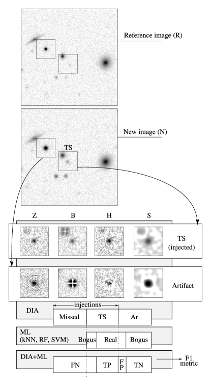
The focus of this work is centered at the task of recovering transient sources from telescope images by combining the Difference Image Analysis and the Machine Learning methods in order to maximize recovery completeness and minimize its contamination. To test the training stage of a ML algorithm, a labeled testing dataset is used to generate predictions, and the performance can be quantified identically to a hypothesis test, by constructing the confusion matrix, as follows: (see Fig. 1)
-
1.
True positives () are the injected transient sources correctly detected and classified as real instances.
-
2.
False positives () are the artifacts in the image differences and the misclassified instances of bogus objects.
-
3.
True Negatives () are the correctly classified bogus
-
4.
False Negatives () are the lost instances due to misclassification or missed by the DIA.
Notice that the components of the confusion matrix can be computed for any detection and classification problem, in particular, either for the results of the DIA or of the DIA+ML, changing the previous definitions accordingly.
Using the values of the confusion matrix we can compute more sophisticated scores, useful to quantify performance metrics for different optimization strategies.
-
1.
Precision measures how many of the classified as positive instances were actually positive. It can be calculated like this: .
-
2.
Recall () or True Positive Rate (TPR) characterizes how many of the positive examples were actually retrieved. This is .
-
3.
False Positive Rate (FPR) is the probability of a false detection, this is .
-
4.
False Negative Rate (FNR) is defined as , and is the rate of lost positive examples.
Precision and recall are useful to check the algorithms performance in this unbalanced class context, where the bogus or artifact objects rate depends on the difference imaging method applied. A more informative value is the score, derived from the precision and recall metrics, which correctly weights the cost of the errors of losing transients as well as detecting artifacts. -measure is the harmonic mean of the and metrics, both equally weighted, and can be used as a final figure of merit. It is computed using , which is the same as and is also a number from 0 to 1. This metric is less sensitive to unbalanced classification scenarios, because it takes an intermediate value between and , but staying closer to the lower value, penalizing the discrepancy of Precision and Recall. At the same time is a metric which does not requires the value of the amount, a quantity we cannot derive from any technique, due to the nature of the problem.
To asses the performance of a trained algorithm, usually new data is used. After the training stage, it is possible to detect cases of over or under training, by using labeled examples which were not processed yet. For this a standard technique named cross–validation, in which the same training set is divided into training and testing subsets, is preferred. This allows to record the mis-classifications and build a confusion matrix. Therefore, we use stratified k-fold cross validation (Witten et al., 2016), which splits the training set in k subsets: k-1 pieces serving for training and the remaining just for validation purpose. The results of the validation of this k classification algorithms trained are the k confusion matrices, one for each fold of test data. The several metrics explained above are then calculated, yielding a confident performance evaluation of the algorithm.
3 Simulated and real datasets
In order to test and compare the different combinations of DIA and ML techniques for transient detection, we explored a range of different observing conditions using a purpose made data-set generating simulated images with transients injections. However these simulations are not completely realistic, so that we also test the combined techniques using observations triggered by GW ALIGO alerts. In both cases the injection of transients allows to asses suitable rate estimates to test the performance of the detection methods.
3.1 Generating a simulated image dataset for ML training
We simulated images using Astromatic Software444https://www.astromatic.net/about, particularly Stuff and SkyMaker (Bertin, 2009), which together can produce realistic images of stars and galaxies, for any given telescope hardware configuration, and including image artifacts such as saturation, spikes, secondary mirror spider shadows, etc. Since it is open source software, it is possible to reproduce the results of the image simulation by introducing the same configurations. We simulated the data in several steps:
-
1.
First we used Stuff to produce a catalog of real objects in the field, including galaxies and stars, containing their positions and real photometric properties, as well as shape parameters.
-
2.
Then this catalog is used to make a fits image using SkyMaker. This is taken as the ”reference image” ().
-
3.
Next some stellar sources (transient) are added to the catalog previously created, at random positions, and with random magnitudes drawn from a fixed Luminosity Function (LF) distribution.
-
4.
The final outcome is a ”new image” () with the transients sources included.
-
5.
The last stage of the simulation is to perform the DIA subtraction between and , and perform the source detection on the resulting difference image.
These steps are repeated once for each point of the explored parameter space, having then, one and one image for each of them. The simulation parameter values cover a relevant range of possible observational configurations, taking into account three aspects, namely, the telescope & site characteristics, the sky stellar background, and the relative location and brightness of the transient with respect to their host galaxy. The simulations expand eight parameters, and each one has associated two images, one corresponds to the reference image and the other is the new image. The values of the parameters used in the images simulations are described in Table 1. Regarding the observational configurations, we considered five parameters, namely, the diameters of the telescope primary and secondary mirrors, the seeing FWHM for and also , the plate scale, and the exposure time. The values of telescope apertures are selected so that they represent the available instruments by our collaboration. The seeing of the images took values of 0.8, 1, and 1.3 arc-seconds, following empirical determination of TOROS future site characteristic values (Fig. 3 in Renzi et al. (2009)). The seeing of the images took values of 1., 1.9, 2.5, motivated by typical and bad observing conditions. The plate scale and exposure times values are chosen according to the available CCD cameras. Regarding the telescope and site characteristics, we include as particular cases, the Estación Astrofísica de Bosque Alegre (EABA), the TOROS pilot instrument (TORITOS) and the projected 0.6-m telescope for the TOROS site. The number and contrast of the stellar sources are described by the stellar density parameter. The range of stellar densities (given by the STARCOUNT_ZP parameter) represents fields of different environments going from typical densities of an mid galactic latitude, and up to densities of less than 5 degrees from the MW disk center at deg of longitude, with a limiting magnitude of . The luminosity distribution of these sources are governed by a power law, with an exponent which took the values of 0.1, 0.5, 0.9 dexp per mag (STARCOUNT_SLOPE parameter in the Skymaker software) Also, we allow the variation of the background surface brightness, using values of 20 and 21 for reference images, typically taken mostly on dark nights, and 20, 19, and even 18 for new images, taken in different conditions. Regarding the host galaxies of the injected transients, we sampled the relative brightness and the angular distance from the host center from uniform distribution in the ranges [-4, 1] magnitudes and [0,5] half light radius, respectively. This allows to explore different transient/host relative configurations, including low relative luminosities and position ranging from the center up to the outer stellar halo. For a given observational configuration (or set of parameters), we define the magnitude range where reliable photometry can be obtained, based on the photometric calibration obtained applying RANSAC (Fischler and Bolles, 1981) robust linear regression on standard sources. The RANSAC method prunes spurious sources, and obtains an estimation of slope and zero point values, not sensitive to outliers, and at the same time also provides a filter mask identifying this outliers.
The explored parameter space may include configurations which are not probable. For instance the combination of a mirror, with seconds exposure time, in a night with a bright background light (i.e. moon light), a large plate scale and a broad seeing. A number of this corner cases are present in the explored configuration space, and in some of this cases simulated images appear completely saturated, and in others the photometric quality is extremely low. This corner cases have been discarded, leaving a total of 26205 groups of , and DIA differenced images.The results shown in the next sections include all sensible points in the explored parameter space, which comprises an heterogeneous combination of image qualities. Nevertheless, the independent photometric calibration of each image informs us the range of validity of flux determination on each configuration making us able to fairly compare results among the whole simulated dataset.
In section 4, we discuss the general trends that result from our analysis. Although our parameter space do not cover all possible configurations for telescope optics and site, we provide the codes that allow to simulated any other observational configuration.
A total of 3272784 transients were injected, placed on top of an extended object (as expected in the case of Kilonovae) with random angular position and distance relative to the host galaxies below 5 half light radius. The simulated galaxies have different morphological types, and also have different redshift values, random orientation and ellipticity and their luminosities are chosen according to a Schechter luminosity function. The magnitudes of the transient objects are disposed with a random offset from the host galaxy, drawn from a uniform distribution, between values -4 and +1 magnitudes.
| TOROS instruments | |||||
| parameter | units | values | eaba | toros | toritos |
| aperture of the telescope | [m] | [0.4, 0.6, 1.54] | 1.54 | 0.6 | 0.4 |
| reference seeing FWHM | [arcsec] | [0.8, 1, 1.3] | 1.3 | 0.8 | 0.8 |
| new image seeing FWHM | [arcsec] | [1.3, 1.9, 2.5] | 2.5 | 1.0 | 1.0 |
| plate scale | [arcsec/pix] | [0.3, 0.7, 1.4] | |||
| exposure times | [sec] | [60, 120, 300] | |||
| stellar density | [stars per sq deg] | [4e3, 8e3, 32e3, 64e3, 128e3, 256e3] | |||
| stellar luminosity distribution exponent | [dexp per mag] | [0.1, 0.5, 0.9] | |||
| background brightness () | [mag per arcsec 2] | [20, 21, 22] | |||
| background brightness () | [mag per arcsec 2] | [18, 19, 20] | |||
| relative brightness from host | r-band magnitudes | sampled from Unif(-4,1) | |||
| angular distance from host | half light radius | sampled from Unif(0, 5) | |||
In the Fig. 1 we present a scheme of the results of the difference image subtraction and the following ML classification of real and bogus transient sources. Besides the reference and new simulated images we show the result of the subtractions performed for this pair of images.
The subtractions were carried out by three different implementations of the techniques introduced above, namely: Zackay, Alard & Lupton, and Bramich algorithms, and we show stamps of bogus and real objects for visual comparison. We also present the resulting image computed as in Eq. 98 from Appendix C of Zackay et al. (2016). As can be seen in the stamps, the properties of the subtractions vary according to the applied methodology. It is worth noticing the shape and the appearance of the same objects after the subtraction has been performed. In the case of the transient source injected we see that every technique presents a point source of almost equal size, except for the S image, which shows an enlarged light distribution. This is due to the nature of the S image, which is a convolution of the Z image with its own PSF. In the second row, we show artifacts originated in the same bright point source. The reason this artifact is consistent in every technique is them failing to correctly match the photometric properties of both and images. In every case we find different structures and these arise because of the intrinsic differences among methods. The artifact in the Z image has a boxy shape due to the PSF determination methodology, in the case of the B image the kernel matches the center of the stellar sources but fails to adequately account for the flux in the wings. Similarly in the case of H we find that the source is still visible, though it lacks a clear structure. In the S case we see an excess of intensity, with a smooth profile, though surrounded by negative pixels, signs of a flux mismatch in the Z image. For the implementation of the Alard and Lupton method we adopted the publicly available HOTPANTS555http://www.astro.washington.edu/users/becker/v2.0/hotpants.html software by Becker (2015) (version 5.1.11). The Bramich implementation is a Python code by the authors, available at https://github.com/toros-astro/ois (version 0.1.14), as well as Zackay et al. implementation, which is also a Python code by the authors available at https://github.com/toros-astro/ProperImage. Both implementations are built upon standard scientific libraries such as NumPy (version used here is 1.15.14), SciPy Jones et al. (2001–) (version 1.1.0) and Astropy (Astropy Collaboration et al., 2013; Price-Whelan et al., 2018) (version 3.0.4),.and run on versions of Python 2.7 as well as 3.6. Also ois and Properimage are fully documented and tested, and they are Open Source, free to the community to use. Many examples and details of the implementation can be found in the documentation at http://optimal-image-subtraction.readthedocs.io and http://properimage.readthedocs.io. This implementation applies a set of pre-processing stages to the images, in order to correctly treat the background, bad pixel masking and interpolation, and PSF determination. It is worth noticing that the Zackay implementation works faster when the exposure times of the reference and new images are equal. In this case there is almost no need for a zero point calibration, which saves computational time. Alard-Lupton implementation is written in C programming language, also it employes a simpler Gaussian PSF assumption, making this method faster than the others by a factor of almost 4X.
3.2 Injection of transient objects on observed images
The simulated images previously used are practical for developing the DIA techniques and generating a training dataset for the bogus/real classification problem. Also this approach allows to explore the dependence of the algorithm performance on different observing settings and transient properties. Nevertheless, this approach is limited by the simplifying hypothesis. In order to take into account the flaws that arise in the observing process and subsequent analysis, we present in this subsection the process of injecting transients sources into real observational images. We used images obtained by the TOROS collaboration as part of the follow up of the triggers during Advanced LIGO science run O2. The images were obtained for the gravitational wave event GW170104, using the Estación Astrofísica Bosque Alegre (EABA) 1.54-m Newtonian telescope. The instrument was set to white light image acquisition, and the CCD used was a Apogee Alta U16. Since the observations were performed hours after the gravitational wave event trigger was received, we had no previous references of the selected targets. The ”reference a posteriori“ methodology was implemented, using images taken over the following months. The objects were selected by cross-correlating and filtering the skymap provided by LSC GCN:20364 and the galaxy catalog from (White et al., 2011), according to the methodology described in the first TOROS follow up paper (Díaz and Collaboration, 2016). The set of observed galaxies comprise NGC1341, NGC1567, NGC1808, ESO0555-022, ESO3564-014, PGC073926, PGC147285, at two epochs separated by eleven months. The images were reduced using a standard image processing, and then co-added for each epoch using the SWarp (Bertin, 2010) public software. The procedure for the subtraction analysis is consistent with the one performed on the simulated dataset. We perform the subtractions using each image twice, once as a reference, and once as a new image. Given the BH-BH merger nature of the GW event (Abbott et al., 2017b) it was not expected any EM emission incoming from this source, and in fact no kilonovae were detected Sanchez et al. (2018). Therefore we decided to inject transients for the intended analysis. In order to simulate a transient object with consistent PSF, we replicated 15 of the actual stars in each frame, inside the true dynamic range of the images. The total number of realizations was 176 using the observed galaxies, yielding a total of 2640 transient injections. The subtraction requires the images to be registered, to that end we developed the python package astroalign666https://github.com/toros-astro/astroalign. This package was inspired by astrometry.net777http://astrometry.net but it does not rely on a prefixed star catalog, instead it aligns two images comparing the asterisms drawn by the brightest stars in the field. These procedures require a complete pipeline for processing and data management as the CORRAL framework (Cabral et al., 2017). This is an open source python package which merges a database connection interface with a Model-View-Controller paradigm, making building complex experimental designs simpler and straightforward, and letting the framework figure out the multi-processing itself. This allows us to write specific processing steps, like those involved in DIA and ML combined analysis, according to an intuitive data handling model. Therefore, we built a similar processing pipeline, using the same sequence of steps, for both the real and the simulated datasets. The completeness and contamination of the transient detection by the DIA pipelines can be increased and reduced, respectively, by the application of the ML algorithms previously introduced. These metrics, among others, were used to rank the transient detection agents, thus allowing to chose the most suitable approach for applications on TOROS images.
4 Comparing transient detection agents
The DIA methods can deliver either direct subtractions (those which return an astronomical image without any convolution process), or convolved subtractions, as the statistic proposed by Zackay et al.. For the direct difference image methods, the transient candidate identifications were performed using SExtractor888https://www.astromatic.net/software/sextractor (version 2.19.5), with the same configuration parameters.
The image, in turn, is a cross-correlation of the difference image with its own PSF, and so the detection of transient candidates is different from the other DIA methodologies. By calculating the statistic from the image and performing a robust determination of its mean and standard deviation (, ), we
can define the significance () of the detection of a candidate in a given pixel as follows:
In Fig.2 it can be seen the distribution of significances for the artifacts and transient sources as well as both cuts of for and in vertical lines, for both datasets.

The chosen threshold of is relaxed with respect to the originally proposed value of by Zackay et al., attempting to detect dim transient sources. Although this increases the number of artifacts, the following ML analysis is expected to label them as bogus. Since SExtractor performs a pre–convolution on every image it scans, we cannot use it on images. Instead we obtained candidates on the images using sep999https://github.com/kbarbary/sep, an open source package capable of running a source extraction without kernel pre–convolution. This software provides photometric measurementes similar to those delivered by SExtractor. The threshold used with this source detection technique is again a limit on over the background.
Therefore we were able to analyze the candidate sources, its photometric properties and parameters measured by SExtractor and sep for every DIA technique, and use this results as features for the ML stage. We end having five DIA transient detection results: detections over Zackay images (Z), over Bramich (B) and over Alard-Lupton differences (A), the three of them provided by SExtractor; detections over using sep (), and detections using a simple pixel treshold (). In what follows (Subsec. 4.1), we explore the main differences between samples of artifacts, real transient sources and missed sources for each DIA method. Since the comparison is based on the very same images, we can directly relate the occurrence of both real transient sources and missed objects among methods, not being this possible in the case of artifacts, since those can be random subtraction errors misidentified as transient candidates. The labeled candidates for Z, B, A and DIA results, and their photometric quantities measured are the inputs of the feature selection process, for training and testing of the ML models aimed at doing the bogus–real classification (Subsec. 4.3).
4.1 Performance of the DIA methods
The fraction of occurrences of the different classes of objects is our first piece of information regarding the subtraction methods performance, prior to any Machine Learning technique application. In Table 2 we show the number of transient sources (TS), missed detections (missed) and artifact sources (Ar), along with the corresponding fractions, TPR, FNR and FPR, respectively. We also report the F1 statistic after the DIA implementation that will be later compared to the same statistic after the ML application.
By definition the values of FNR and TNR always add up to one, and FPR can be any number, since the normalization is over the total number of injected sources. Regarding the rates of recovered transient sources (TPR), we read that there is variability on the results for different techniques. There is a baseline of 50% for every technique, and a top value of 93%, finding intermediate values in the simulated as well in the real dataset. The number of missed objects is larger in the case of the simulation, since we injected transients in a larger number of simulated images, covering a wide range of experimental configuration (as indicated in Table 1).
For the simulated dataset we can read that Bramich finds less transients, and at the same time produces less artifacts. For the real dataset it finds more transients than any other technique, and produces a relatively low amount of artifacts. The technique which finds more transient sources is , with a relatively low number of artifacts for the simulated dataset. In the case of the real dataset the scenario is the opposite. The method which generates more artifacts in the simulated case is Alard-Lupton, yielding more than twice the amount of false detections than Zackay technique. In case of the real dataset this happens for the which has a FPR of 200, and Zackay generates less artifacts than any other DIA method. This behaviour can be explained with the tendency of of finding local maximae in the edges of images, or near bright sources, an issue we would like to address in the future.
In the simulated dataset we find that the statistic is systematically higher than the real dataset results. This is mostly due to extremely high FPR we measure in the latter. It is clear that we have more sources of confusion in the real images, this could explained by the presence of instrumental defects on the CCD camera used, poor flat field calibration, and correlated noise coming from the stacking procedure. These effects are not straightforward to include in the simulations therefore we can think of them as a representation of an optimistic case scenario, in comparison to the observations.
| Simulated dataset | |||||||
|---|---|---|---|---|---|---|---|
| TS | Missed | Ar | TPR | FNR | FPR | F1 | |
| Z | 1,933,065 | 1,339,719 | 3,170,089 | 0.59 | 0.41 | 0.97 | 0.46 |
| B | 1,596,713 | 1,676,071 | 1,979,948 | 0.49 | 0.51 | 0.60 | 0.47 |
| A | 1,971,291 | 1,301,493 | 5,537,472 | 0.60 | 0.40 | 1.70 | 0.37 |
| 2,180,390 | 1,092,394 | 2,456,876 | 0.67 | 0.33 | 0.75 | 0.55 | |
| 2,092,625 | 1,180,159 | 2,700,107 | 0.64 | 0.36 | 0.83 | 0.52 | |
| Real dataset | |||||||
| TS | Missed | Ar | TPR | FNR | FPR | F1 | |
| Z | 2296 | 344 | 25914 | 0.87 | 0.13 | 9.8 | 0.15 |
| B | 2468 | 172 | 47731 | 0.93 | 0.07 | 18.1 | 0.09 |
| A | 2179 | 461 | 110,025 | 0.83 | 0.17 | 41.7 | 0.04 |
| 2099 | 541 | 128,820 | 0.80 | 0.20 | 48.8 | 0.03 | |
| 2043 | 597 | 528,927 | 0.77 | 0.23 | 200.4 | 0.008 | |
4.2 Analyses of the DIA results
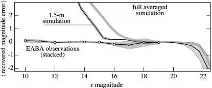
In order to compare the photometric properties of the transient candidates for every DIA method, we performed a photometric calibration with the flux of the simulated astronomical sources, by using a robust linear regression as already detailed in Sec. 3. The measured magnitudes of the transients recovered in the simulation generated images shows agreement among the different DIA methods. We show in the Fig. 3 the mean and the standard error of the difference between the injected and measured magnitudes of the transients recovered in the simulated images, as a function of the transient r-magnitude. We also show in this Figure the results for transients injected on EABA observations, and the subset of simulated images that are closest to the observing configuration of the EABA telescope and site. The difference between the EABA observations and the corresponding simulation arises because of several factors. Most importantly is that the real dataset images are stacks of images, and this largely enhances its dynamic range, allowing to observe bright sources without saturation, and at the same time, sources at magnitudes fainter than 17 with an good signal to noise ratio. In the simulations, the aperture photometry might not be able to ideally capture the true flux value of the bright saturated or enlarged sources. Prior to reaching the saturation limit, the linearity of the CCD response is lost, progressively deviating flux measurements from true values. The limiting magnitude difference between simulations and real data are due to the actual performance of the EABA instrument, and the atmospheric conditions during the nights of O2 follow up observations. Taking this into account, it is worth noticing that the simulated and observed images are consistent within a range of approximately 5 magnitudes.
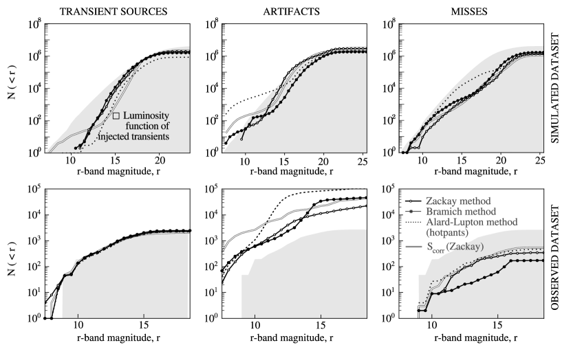
We also studied several statistics for each class of object, trying to gain insight into their properties. The Cumulative Luminosity Function for each class in the simulated dataset is displayed on the top row of the Fig. 4, where it can be seen that for the transient sources the methods are roughly equivalent. We find that for the magnitude range the methods behave similarly, but Zackay and S-Corr have more transient sources detected than the rest of the techniques. In this faint end of the luminosity function the main reason for losing objects is the detection limits. In the bright end however, there is not a clear pattern, and besides the true missed objects, the already discussed errors in the magnitude measurements for bright objects due to saturation could increase the discrepancy with the simulated magnitude values.
In the case of the artifacts, both in the simulated and observed dataset, we find similar behaviour in the DIA techniques, although it is worth to notice that the accumulated number of objects is in disagree with the reported figures in Tab. 2, this is due to the fact that many artifact sources present flux measurements without astrophysical meaning. The values of magnitudes calculated for a portion of the artifacts fall outside the range presented in the Fig. 4.
The right panel of Fig. 4 top row, corresponding to the missed objects in the simulations, shows that all methods fail to recover an important number of sources fainter than 21 magnitudes, and also objects brighter than 12 magnitudes. Since this missed, and trasient sources sets of objects are the complement of each other we find similar explanations for the bi modality of lost sources and the deficits of injected recovered objects. Particularly S-Corr is the method which lose less injected sources, followed by Alard-Lupton, although the latter losses objects in the whole range presented, in contrast with the other methods. As a comparison with the real dataset, we find that there is not such gap in between the faint and bright end of the missed objects luminosity function, but instead a smooth ever increasing distribution is observed. In the real dataset, we have a different picture, with every method losing objects, almost equally, except for the Bramich method, whose distribution seems to be fainter, and shows accumulated numbers below every other technique. We also observe a slight increase in the number of objects lost for the S-Corr compared to the rest of the techniques, although is should be recalled that there is a big gap between the sample sizes of simulated and real datasets.
In certain way a higher contamination of bogus may be acceptable since Machine Learning algorithms could separate them from the true interesting candidates, and on the other side, a high FNR is quite undesirable since those candidates are “lost forever”. This compromise should be constrained in advance, and shouldn’t be taken for granted. Every algorithm could be optimized by using iterations or other supplementary techniques, moving the scenario to a more favorable ratios scenario.
4.3 Machine Learning Results
As explored above, we have photometric properties for the detected candidates in the several DIA images. On top of this we also have shape properties, as well as high order statistical moments on their light distributions provided by SExtractor -an in case sep-. This labeled dataset together with the mentioned features, constitutes the input instances for training and testing ML algorithms in the task of classifying the bogus and real objects.
In order to asses the different scenarios we simulated, our machine learning experiments were conducted in several steps:
-
1.
We grouped the dataset in terms of three simulation configuration values: the mirror diameter of the telescope, the exposure time, and the seeing of the new image. This gave us 27 subsets of data, where we conducted identical and independent experiments.
-
2.
Each experiment was carried out firstly by splitting the dataset into a training and final testing set, with a 20%-80% proportion respectively, due to the enormous amount of data available for training.
-
3.
The training subset is used to perform feature preprocess and selection, and to perform a k-fold cross validation performance measure for three ML algorithms: k-Nearest Neighbors, Random Forests, and linear Support Vector Machines.
-
4.
We calculated the confusion matrix for the ML classification (Bogus–Real), and combined it with the DIA performance metrics, in order to rank the DIA+ML methodologies using an overall figure of merit. This is done by deriving a confusion matrix from the injected sources, through the DIA (Missed, TS, Artifacts), to its final DIA+ML classification results (FN, TP, FP, and TN), such as illustrated in Fig. 1.
The used Machine Learning algorithms as previously stated were:
-
1.
k-Nearest Neighbors, using 7 neighbors, with uniform weights and euclidean distances (using scaled feature values).
-
2.
Random Forest, with 800 trees, with up to 7 features per tree, stopping the tree growing if less than 20 examples per leaf, using a Gini impurity criterion.
-
3.
Support Vector Machines, using L2 norm penalization, with a tolerance parameter of , solving the dual optimization problem, and weighting the classes if unbalanced for their frequency.
All the configurations for the ML algorithms correspond to Sci-Kit Learn version .
4.3.1 The feature selection process
We performed a preprocessing of the features, by scaling them to zero mean, and unit variance. Afterwards we applied univariated analysis by using a variance threshold cut of , pruning constant features. Following this simple treatment we used three different feature selection strategies, adapted to each ML algorithm tested .
To calculate the importances for kNN algorithm, we used the mutual information of the features and the target class, selecting the percentile as a threshold cut.
For RandomForest we applied a feature selection process following Bloom et al. (2012), using a RandomForest training stage, and picking those features that were the most informative in the majority of the individual trees. To avoid bias in the selection we pruned the correlated features, and afterwards we followed the methodology described in associated Python package rfpimpin a 10-fold cross validation experiment. To determine the unimportant features we added to the training dataset a uniformly distributed random variable. Using this procedure we can set the zero value of the scale as the importance of this Random feature. We calculated the mean and standard deviation of the 10 values obtained in the 10-fold experiment, tossing away those features consistent with the values obtained for the Random one.
For Support Vector Machines we applied a Recursive Feature Elimination on a 6-fold experiment, using an elimination step of , and choosing as the scoring metric to maximize.
4.3.2 Evaluation of DIA+ML algorithms
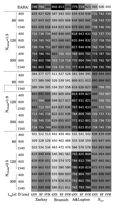
In Fig. 5 we show a heatmap of values of statistic (scaled by a factor of ) for the results of the 12 DIA+ML combinations (4 DIA techniques and 3 ML algorithms). The map is obtained by grouping several possible instrumental configurations, spanning the dimensions of the FWHM for the new image () measured in arcseconds, the exposure time () measured in seconds, and the diameter of the primary mirror () in cm, and performing the ML train–test experiments on each group. This covers a wide range of instruments, from small to middle size telescopes, and from good to poor observing conditions. There exists though, several possible configurations which are not covered by our analysis, designed mostly for TOROS collaboration available instruments. Nevertheless the analysis is valid for numerous transient search science collaborations with instruments falling within the range of our simulation parameters, such as (piofthesky, black gem, assassn, los alerces, catalina sky survey, etc). It is also worth noticing that for each of the 27 instrumental configurations analyzed we are mixing the combination of values of the rest of the simulation parameters (listed in Tab. 1), and in consequence including several dissimilar transient detection scenarios into the same ML experiment.
This result shows an expected dependence in the simulation parameters, clearly favouring longer exposure times and smaller seeing FWHM for the new image, there is also weaker but present dependence on mirror size. The strongest dependence of the value holds with the DIA technique applied. It is clear that independently of the ML used Alard & Lupton DIA method has better performance in terms of statistic in the simulations, followed by Zackay’s techniques (including ). There is no major difference among ML algorithms for a given DIA technique, but a small advantage seems to be obtained when using RandomForest.
We also include the values of for the real dataset in the top of the map, which can be compared to the highlighted equivalent simulation. In the observed dataset we find that generally Bramich is better ranked, and the best DIA+ML technique is its combination with kNN. Notice that the overall for this DIA method is much better in this observed dataset than in the simulations. However the range of values for the ML+DIA combination are comparable, despite the difference in the values of DIA only.
In order to better compare the performances reported in Fig. 5 we have marginalized over the groups of instrumental configurations, showing the quartiles of the distribution of values in the Fig. 6. In order to compare these values before and after ML classification we also include as horizontal lines the quartiles of the distribution of the values obtained in each group after the application of the DIA methods only. It is clear from this figure that Alard&Lupton technique is better ranked than any other DIA method, and at the same it experiences the largest boost in performance after the application of any ML algorithm. We also show in dots the results for the observed dataset and in horizontal dotted line we also include the value for the corresponding DIA methodology (see Tab. 2). In the real dataset we find that the combinations which make use of kNN and RandomForest algorithms are signficantly better ranked than SVM combinations. In general Bramich DIA technique results in better performance as measured by statistic, comparable to the best values obtained in the simulations. However we notice that this result is linked mostly to the improvement that ML algorithm provides, which is larger than in the simulated dataset. It is noticeable also, that Alard&Lupton results are consistent between simulation and real dataset within the uncertanties, being this also consistent with the Bramich results for the real dataset case. This will be further explored when the TOROS collaboration instrument data aquisition period begins, and larger collections of images are available.
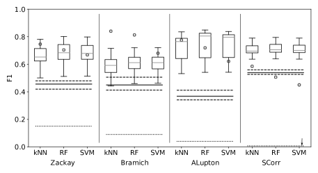
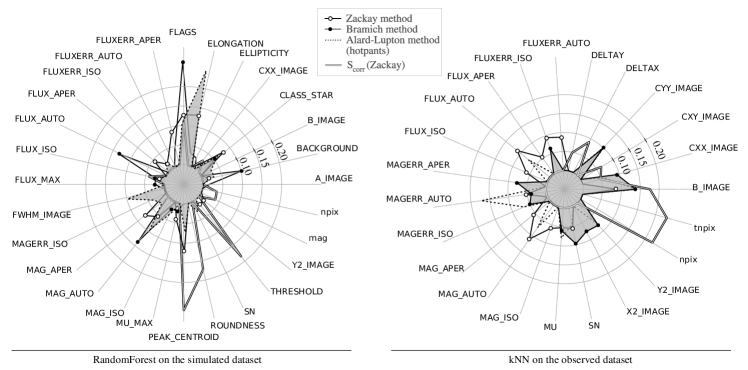
As a global result we report that the best combination of DIA+ML for the simulated dataset is Alard & Lupton implementation Hotpants, and RandomForest. For the real dataset in turn we find that the best performance is with Bramich DIA combined with kNN machine learning algorithm. For these two cases we present the selected features and their normalized relative importances in Fig. 7. The included features in this figure sum up 90% of the total importance calculated for the whole set of selected features in each DIA+ML case. We can see that in the simulation the 5 most important features in the case of the best ranked DIA+ML for the simulated dataset, that is A&Lupton, are in order ELONGATION, FLAGS, FWHM_IMAGE, MAG_AUTO and CLASS_STAR. In case of the real dataset, for Bramich+kNN the 5 most important features are in order B_IMAGE, CXX_IMAGE, CYY_IMAGE, SN, FLUXERR_ISO. The details on the calculation and meaning of each feature are included in Appendix A. The disagreement among the maps of importance might be explained considering the differences in the DIA+ML algorithm, and its feature selection procedure. Still, we can detect that the most important features represent as expected, shape and brightness parameters.
In order to gain some insights on the simulated dataset, we explored some of the dependences of the metrics of performance with the parameters of the injections.
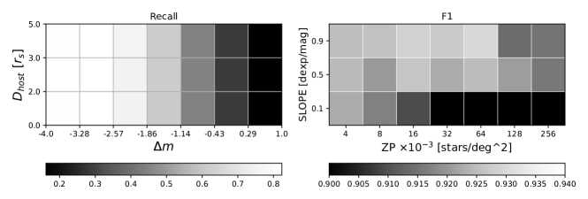
In the Fig. 8 we show the values of Recall and metric scores, as two dimensional maps, for two pairs of the simulation parameters, for the A&Lupton+RandomForest technique. The first one, in left panel, shows the dependance of with the values of relative position and brightness to the host galaxy. This maps clearly shows a strong dependence of the Recall of the final ML+DIA on the relative brightness, and at the same time shows no dependence on the distance to the host galaxy center. The second map, in right panel, shows the values as a function of the parameters of the stellar luminosity function of the star field on the images: STARCOUNT_SLOPE and STARCOUNT_ZP. As explained in Sec. 3.1 the stellar luminosity function is a power law, and the exponent is the value of STARCOUNT_SLOPE, the STARCOUNT_ZP parameter is the total density of stars in the field (see Tab. 1). This map indicates that in a dense environment the is lower, indicating the number of stars in the image as source of confusion for the DIA+ML technique. At the same time a lower slope, which traduces into in more bright stars at a fixed total density, pushes the scoring to lower values. It is clear then that dense stellar fields, like the ones in the galactic plane, are places where a decrese in the performance of the DIA+ML is expected. These class of studies are possible to evaluate by using a multi parameter simulation, like the one carried out.
5 Conclusions
We developed open source tools for image subtraction following the DIA techniques from Bramich (2008) and Zackay et al. (2016). We also made use of HOTPANTS implementation of Alard-Lupton algorithm. The Python packages developed, together with HOTPANTS, were mounted on top of a CORRAL data processing pipeline, in order to systematically perform image subtractions with transient candidate injections. The images used for this were drawn from EM counterpart search, carried out by TOROS during O2 LIGO-Virgo-Scientific collaboration science observing run in 2017. This observations were performed during January and November, using the “reference a posteriori” methodology previously applied by TOROS collaboration. Additionally we developed comprehensive simulations of images, exploring a multi dimensional parameter space of instrumental configuration as well as observing conditions, as detailed in Tab. 1, generating millions of transient injected on top of extended sources over several thousands of images. The nature of the injected transients does not include moving objects, or stellar variability, focusing the analysis on Kilonova/Supernova detection scenarios.
The mentioned pipelines measured the ratios of recovery of injected transients, as well the source contamination and loss for each DIA algorithm. We also compared their photometric results, including the image photometry. In order to separate the true transient candidates from the spurious artifact detections we applied Machine Learning algorithms, trained with data generated by our pipeline. We carried out a feature selection stage, and completed a cross validation train-test experiment, in order to calculate score metrics such as Precision and Recall, useful to compare performances in an unbalanced class context, and ranked the methodologies by combining them in the statistic.
The comparison in the simulated and real data showed that the scenario was of relevance in the performance of the different combination of methodologies, bringing differences which can relate to the techniques as well as the nature of data used. Our results shows that Zackay’s image subtraction techniques, including , are more suitable for transient detection as a standalone technique. However it is clear that the Machine Learning algorithms are key to complete the task of selecting the relevant transient candidates, by setting apart the artifacts which contaminate and are uninteresting. After the application of these algorithms, and looking at the final performance metric we conclude that, among the DIA+ML combinations tested, the better ranked technique were: in the real EABA images dataset Bramich+kNN, and in the simulated dataset A&Lupton+RandomForest. Although we find consistency, within the uncertanties, among every ML applied technique in the simulated data, for every DIA method. This is also valid between the real and simulated dataset, for the A&Lupton and Zackay case. For these selected methods we also report the more important features, determined by Random Forest permutation importance in the case of the simulations, and by univariated analysis in the case of the real dataset.
Seizing the large and complex simulation generated, we analyzed the dependency of the Recall metric on the environment of the injected transients, in relation to the host galaxy, and the stellar field present in the simulated images. Concluding that is more likely to generate artifacts and miss a fraction of transient objects in a dense and bright stellar field, and also to miss a greater fraction of detections if the contrast in brightness with the host galaxy is small, independently of its spatial relative location.
These results are very important for the development of the data processing pipeline of the TOROS collaboration which comprises different telescopes and instruments. A future extension of this work is to tackle the genuine transient time-series astrophysical classification for large amounts of data.
Simulation results and data used in this work are available to the community, in the format of candidates catalog tables at O. (2019)101010 https://zenodo.org/record/2658714.
Acknowledgements
This work was partially supported by the Consejo Nacional de Investigaciones Científicas y Técnicas (CONICET, Argentina) and the Secretaría de Ciencia y Tecnología de la Universidad Nacional de Córdoba (SeCyT-UNC, Argentina). M.B and M.D. acknowledge NSF support through grant NSF-HRD 1242090. JLNC is grateful for financial support received from the GRANT PROGRAMS FA9550-15-1-0167 and FA9550-18-1-0018 of the Southern Office of Aerospace Research and development (SOARD), a branch of the Air Force Office of the Scientific Research International Office of the United States (AFOSR/IO). The authors also thank for their kind suggestions and commentaries to D. Bramich and B. Zackay.
This research has made use of the adsabs.harvard.edu/, Cornell University xxx.arxiv.org repository, the SIMBAD database, operated at CDS, Strasbourg, France.
References
References
- Abbott et al. (2017a) Abbott, B.P., Abbott, R., Abbott, T.D., Acernese, F., Ackley, K., Adams, C., Adams, T., Addesso, P., 2017a. Multi-messenger observations of a binary neutron star merger. ApJ 848, L12. URL: http://stacks.iop.org/2041-8205/848/i=2/a=L12.
- Abbott et al. (2017b) Abbott, B.P., Abbott, R., Abbott, T.D., Acernese, F., Ackley, K., Adams, C., Adams, T.e.a. (LIGO Scientific and Virgo Collaboration), 2017b. Gw170104: Observation of a 50-solar-mass binary black hole coalescence at redshift 0.2. Phys. Rev. Lett. 118, 221101. URL: https://link.aps.org/doi/10.1103/PhysRevLett.118.221101, doi:10.1103/PhysRevLett.118.221101.
- Abbott and Collaboration (2016) Abbott, B.P., Collaboration, T.L.S. (LIGO Scientific Collaboration and Virgo Collaboration), 2016. Observation of gravitational waves from a binary black hole merger. Phys. Rev. Lett. 116, 061102. URL: http://link.aps.org/doi/10.1103/PhysRevLett.116.061102, doi:10.1103/PhysRevLett.116.061102.
- Alard and Lupton (1998) Alard, C., Lupton, R.H., 1998. A Method for Optimal Image Subtraction. ApJ 503, 325–331. doi:10.1086/305984, arXiv:astro-ph/9712287.
- Astropy Collaboration et al. (2013) Astropy Collaborationet al., 2013. Astropy: A community Python package for astronomy. aap 558, A33. doi:10.1051/0004-6361/201322068, arXiv:1307.6212.
- Barnes et al. (2016) Barnes, J., Kasen, D., Wu, M.R., Martínez-Pinedo, G., 2016. Radioactivity and Thermalization in the Ejecta of Compact Object Mergers and Their Impact on Kilonova Light Curves. AJ 829, 110. doi:10.3847/0004-637X/829/2/110, arXiv:1605.07218.
- Becker (2015) Becker, A., 2015. HOTPANTS: High Order Transform of PSF ANd Template Subtraction. Astrophysics Source Code Library. arXiv:1504.004.
- Bertin (2009) Bertin, E., 2009. SkyMaker: astronomical image simulations made easy. Mem. Soc. Astron. Italiana 80, 422.
- Bertin (2010) Bertin, E., 2010. SWarp: Resampling and Co-adding FITS Images Together. Astrophysics Source Code Library. arXiv:1010.068.
- Bloom et al. (2012) Bloom, J. S. et al., 2012. Automating Discovery and Classification of Transients and Variable Stars in the Synoptic Survey Era. PASP 124, 1175. doi:10.1086/668468, arXiv:1106.5491.
- Bramich et al. (2016) Bramich, D., Horne, K., Alsubai, K., Bachelet, E., Mislis, D., Parley, N., 2016. Difference image analysis: automatic kernel design using information criteria. Monthly Notices of the Royal Astronomical Society 457, 542–574.
- Bramich (2008) Bramich, D.M., 2008. A new algorithm for difference image analysis. MNRAS 386, L77–L81. doi:10.1111/j.1745-3933.2008.00464.x, arXiv:0802.1273.
- Breiman (2001) Breiman, L., 2001. Random forests. Machine learning 45, 5–32.
- Cabral et al. (2017) Cabral, J.B., Sánchez, B., Beroiz, M., Domínguez, M., Lares, M., Gurovich, S., Granitto, P., 2017. Corral framework: Trustworthy and fully functional data intensive parallel astronomical pipelines. Astronomy and Computing 20, 140–154. doi:10.1016/j.ascom.2017.07.003, arXiv:1701.05566.
- Cover and Thomas (2012) Cover, T.M., Thomas, J.A., 2012. Elements of information theory. John Wiley & Sons.
- Díaz and Collaboration (2016) Díaz, M.C., Collaboration, T., 2016. GW150914: First Search for the Electromagnetic Counterpart of a Gravitational-wave Event by the TOROS Collaboration. ApJ 828, L16. doi:10.3847/2041-8205/828/2/L16, arXiv:1607.07850.
- Díaz et al. (2017) Díaz, M. C. et al., 2017. Observations of the first electromagnetic counterpart to a gravitational-wave source by the toros collaboration. ApJ 848, L29. URL: http://stacks.iop.org/2041-8205/848/i=2/a=L29.
- Djorgovski et al. (2010) Djorgovski, S.G., Drake, A.J., Mahabal, A.A., Graham, M.J., Donalek, C., Beshore, E., Larson, S., 2010. Exploring the Variable Sky with the Catalina Real-Time Transient Survey, in: The First Year of MAXI: Monitoring Variable X-ray Sources, p. 32.
- Domingos (2012) Domingos, P., 2012. A few useful things to know about machine learning. Commun. ACM 55, 78–87. URL: http://doi.acm.org/10.1145/2347736.2347755, doi:10.1145/2347736.2347755.
- Fischler and Bolles (1981) Fischler, M.A., Bolles, R.C., 1981. Random sample consensus: A paradigm for model fitting with applications to image analysis and automated cartography. Commun. ACM 24, 381–395. URL: http://doi.acm.org/10.1145/358669.358692, doi:10.1145/358669.358692.
- Fortson et al. (2012) Fortson, L. et al., 2012. Galaxy Zoo: Morphological Classification and Citizen Science. CRC Press, Taylor and Francis Group. pp. 213–236.
- Guyon et al. (2002) Guyon, I., Weston, J., Barnhill, S., Vapnik, V., 2002. Gene selection for cancer classification using support vector machines. Machine Learning 46, 389–422. URL: https://doi.org/10.1023/A:1012487302797, doi:10.1023/A:1012487302797.
- Hastie et al. (2001) Hastie, T., Tibshirani, R., Friedman, J., 2001. The Elements of Statistical Learning. Springer Series in Statistics, Springer New York Inc., New York, NY, USA.
- Ivezic and for the LSST Collaboration (2008) Ivezic, for the LSST Collaboration, 2008. LSST: from Science Drivers to Reference Design and Anticipated Data Products. ArXiv e-prints arXiv:0805.2366.
- Jones et al. (2001–) Jones, E., Oliphant, T., Peterson, P., et al., 2001–. SciPy: Open source scientific tools for Python. URL: http://www.scipy.org/. [Online; accessed ¡today¿].
- Kasen et al. (2013) Kasen, D., Badnell, N.R., Barnes, J., 2013. Opacities and Spectra of the r-process Ejecta from Neutron Star Mergers. AJ 774, 25. doi:10.1088/0004-637X/774/1/25, arXiv:1303.5788.
- Law et al. (2009) Law, N. M. et al., 2009. The Palomar Transient Factory: System Overview, Performance, and First Results. PASP 121, 1395. doi:10.1086/648598, arXiv:0906.5350.
- LSST Science Collaboration et al. (2009) LSST Science Collaborationet al., 2009. LSST Science Book, Version 2.0. ArXiv e-prints arXiv:0912.0201.
- Mitchell (1997) Mitchell, T.M., 1997. Machine Learning. 1 ed., McGraw-Hill, Inc., New York, NY, USA.
- Neyman and Pearson (1933a) Neyman, J., Pearson, E.S., 1933a. On the problem of the most efficient tests of statistical hypotheses. Philosophical Transactions of the Royal Society of London A: Mathematical, Physical and Engineering Sciences 231, 289–337. URL: http://rsta.royalsocietypublishing.org/content/231/694-706/289, doi:10.1098/rsta.1933.0009, arXiv:http://rsta.royalsocietypublishing.org/content/231/694-706/289.full.pdf.
- Neyman and Pearson (1933b) Neyman, J., Pearson, E.S., 1933b. The testing of statistical hypotheses in relation to probabilities a priori. Mathematical Proceedings of the Cambridge Philosophical Society 29, 492–510. doi:10.1017/S030500410001152X.
- O. (2019) O., S.B., 2019. HDF5 Table for Machine Learning on Difference image analysis. URL: https://doi.org/10.5281/zenodo.2658714, doi:10.5281/zenodo.2658714.
- Oelkers et al. (2015) Oelkers, R. J. et al., 2015. Difference Image Analysis of Defocused Observations With CSTAR. AJ 149, 50. doi:10.1088/0004-6256/149/2/50, arXiv:1410.4544.
- Oelkers et al. (2013) Oelkers, R.J., Wang, L., Zhou, J., Macri, L.M., CSTAR, PLATO, 2013. Difference Image Analysis of 2009 CSTAR Observations from Dome A in Antarctica, in: American Astronomical Society, AAS Meeting 221, id.352.23.
- Pearson (1901) Pearson, K., 1901. On lines and planes of closest fit to systems of points in space. Philosophical Magazine 2, 559–572.
- Pedregosa et al. (2011) Pedregosa, F. et al., 2011. Scikit-learn: Machine learning in python. Journal of Machine Learning Research 12, 2825–2830.
- Phillips and Davis (1995) Phillips, A.C., Davis, L.E., 1995. Registering, psf-matching and intensity-matching images in iraf, in: Astronomical Data Analysis Software and Systems IV, volume 77 of ASP Conference Series. p. 297.
- Price-Whelan et al. (2018) Price-Whelan, A. M. et al., 2018. The Astropy Project: Building an Open-science Project and Status of the v2.0 Core Package. aj 156, 123. doi:10.3847/1538-3881/aabc4f.
- Rau et al. (2009) Rau, A., Kulkarni, S.R., Law, N.M., Bloom, J.S., Ciardi, D., Djorgovski, G.S.e.a., 2009. Exploring the Optical Transient Sky with the Palomar Transient Factory. PASP 121, 1334. doi:10.1086/605911, arXiv:0906.5355.
- Renzi et al. (2009) Renzi, V. et al., 2009. Caracterización astronómica del sitio cordón macón en la provincia de salta. Boletín de la Asociación Argentina de Astronomía 52, 285–288.
- Sanchez et al. (2018) Sanchez, B., Beroiz, M., Diaz, M., Macri, L., M., D., 2018. No bh em emission. in prep. .
- Sedaghat and Mahabal (2017) Sedaghat, N., Mahabal, A., 2017. Effective Image Differencing with ConvNets for Real-time Transient Hunting. ArXiv e-prints arXiv:1710.01422.
- Strobl et al. (2008) Strobl, C., Boulesteix, A.L., Kneib, T., Augustin, T., Zeileis, A., 2008. Conditional variable importance for random forests. BMC Bioinformatics 9, 307. URL: https://doi.org/10.1186/1471-2105-9-307, doi:10.1186/1471-2105-9-307.
- Strobl et al. (2007) Strobl, C., Boulesteix, A.L., Zeileis, A., Hothorn, T., 2007. Bias in random forest variable importance measures: Illustrations, sources and a solution. BMC Bioinformatics 8, 25. URL: https://doi.org/10.1186/1471-2105-8-25, doi:10.1186/1471-2105-8-25.
- White et al. (2011) White, D.J., Daw, E.J., Dhillon, V.S., 2011. A list of galaxies for gravitational wave searches. Classical and Quantum Gravity 28, 085016. URL: http://stacks.iop.org/0264-9381/28/i=8/a=085016.
- Witten et al. (2016) Witten, I.H., Frank, E., Hall, M.A., Pal, C.J., 2016. Data Mining: Practical machine learning tools and techniques. Morgan Kaufmann.
- Zackay and Ofek (2017a) Zackay, B., Ofek, E.O., 2017a. How to COADD Images. I. Optimal Source Detection and Photometry of Point Sources Using Ensembles of Images. ApJ 836, 187. doi:10.3847/1538-4357/836/2/187, arXiv:1512.06872.
- Zackay and Ofek (2017b) Zackay, B., Ofek, E.O., 2017b. How to COADD Images. II. A Coaddition Image that is Optimal for Any Purpose in the Background-dominated Noise Limit. ApJ 836, 188. doi:10.3847/1538-4357/836/2/188, arXiv:1512.06879.
- Zackay et al. (2016) Zackay, B., Ofek, E.O., Gal-Yam, A., 2016. Proper Image Subtraction: Optimal Transient Detection, Photometry, and Hypothesis Testing. ApJ 830, 27. doi:10.3847/0004-637X/830/1/27, arXiv:1601.02655.