Abstract

We study the parameter dependence of numerical results obtained by the tensor renormalization group. We often observe an irregular behavior as the parameters are varied with the method, which makes it difficult to perform the numerical derivatives in terms of the parameter. With the use of two-dimensional Ising model we explicitly show that the sharp cutoff used in the truncated singular value decomposition causes this unwanted behavior when the level crossing happens between singular values below and above the truncation order as the parameters are varied. We also test a smooth cutoff, instead of the sharp one, as a truncation scheme and discuss its effects.

I Introduction

Tensor renormalization group (TRG) is a promising approach that can solve the sign problem inherent in the Monte-Carlo simulations. Since it was proposed in two-dimensional Ising model Levin:2006jai , many studies have been carried out for various models of lattice field theories Shimizu:2012wfa ; Shimizu:2014uva ; Unmuth-Yockey:2014iga ; Shimizu:2014fsa ; Takeda:2014vwa ; Kawauchi:2016xng ; Meurice:2016mkb ; Sakai:2017jwp ; Yoshimura:2017jpk ; Shimizu:2017onf ; Kuramashi:2018mmi ; Kadoh:2018hqq . In TRG, the truncated singular value decomposition (SVD) is used to define a coarse-grained tensor, which is given in a manner of sharp cut-off such that the $D_{\mathrm{cut}}$ largest singular values and corresponding singular vectors are kept and the others are thrown away. Although the cutoff yields possible systematic errors, it is expected that the result should converge to the correct value as $D_{\mathrm{cut}}$ increases.

The results of TRG, however, do not smoothly depend on the parameters in the theory. They often show irregular behavior at some parameters off the critical point. This behavior is controlled by $D_{\mathrm{cut}}$, but for small $D_{\mathrm{cut}}$ it is difficult to obtain the smooth parameter dependence of the results, to which we may apply the numerical derivative with respect to the parameter. We can of course obtain a satisfactory result for a simple model such as two-dimensional Ising model taking a sufficiently large $D_{\mathrm{cut}}$ to avoid such misbehavior. However, it would be difficult to increase $D_{\mathrm{cut}}$ for general lattice theories with multi-dimensional fields so that it should be important to understand and avoid the irregular behavior of the results.

In this paper we investigate the origin of the irregular parameter dependence shown in the TRG results. We present some numerical evidence that it is caused by the level crossing between singular values within and beyond the sharp truncation as the parameters are varied. In this sense the irregular behavior is inevitable for the TRG method with the sharp cutoff. In order to obtain a hint of improving the behavior, we also test other cutoff schemes such as a smooth cutoff.

The rest of this paper is organized as follows. In Sec. II we review the standard TRG method with the sharp cutoff in two-dimensional Ising model with sample numerical results. The mechanism of irregular behavior is explained in detail with some numerical evidence in Sec. III. We also test other cutoff schemes. Our conclusions are summarized in Sec. IV.

II TRG in two dimensional Ising model

We briefly review the TRG method in two-dimensional Ising model presenting a couple of numerical results for later convenience.

II.1 Numerical procedures in TRG

We consider a two-dimensional square lattice whose sites are labeled by $n=(n_{1},n_{2})$ for $n_{1},n_{2}\in\mathbb{Z}$. The spin variable $\sigma_{n}$ assigned on the site $n$ takes the discrete values $\sigma_{n}\in\{1,-1\}$. Two dimensional Ising model is then defined by the Hamiltonian

$${\cal H}=-J\sum_{\langle i,j\rangle}\sigma_{i}\sigma_{j},$$ (1)

where $\langle i,j\rangle$ denotes possible pairs of the nearest neighbor sites and $J$ is the coupling constant.

The partition function $Z={\rm Tr}\,{\rm e}^{-\beta{\cal H}}$ with the inverse temperature $\beta=1/T$ can be expressed as a tensor network form:

$$Z=\sum_{i,j,k,l,\dots}T_{ijkl}\ldots$$ (2)

where

$$T_{ijkl}=e^{\beta J(ij+jk+kl+li)}$$ (3)

for $i,j,k,l=-1,1$.

Let us denote the bond dimension of $T_{ijkl}$ as $N$ for the sake of argument. Note that the initial tensor of Eq. (3) is defined with $N=2$. We apply the truncated SVD to $T_{ijkl}$:

$$T_{ijkl} \approx\sum_{m=1}^{D_{\mathrm{cut}}}U_{(ij)m}\lambda_{m}V^{\dagger}_{m(kl)}$$ (4)

$$T_{ijkl} \approx\sum_{m=1}^{D_{\mathrm{cut}}}U^{\prime}_{(li)m}\lambda^{\prime}_{m}{V^{\prime}}^{\dagger}_{m(jk)},$$ (5)

where $T_{ijkl}$ is treated as a matrix with the column $(ij)$ and row $(kl)$ in Eq. (4) and a matrix with the column $(li)$ and row $(jk)$ in Eq. (5). The above expressions assume the case of $N^{2}>D_{\mathrm{cut}}$, while $D_{\mathrm{cut}}$ in Eqs. (4) and (5) is replaced by $N^{2}$ for $N^{2}\leq D_{\mathrm{cut}}$ without any truncation. We apply the decomposition of Eq. (4) to the tensors at even sites defined by mod($n_{1}+n_{2}$,2)=0 and that of Eq. (5) to ones at odd sites with mod($n_{1}+n_{2}$,2)=1. Here $U,V,U^{\prime},V^{\prime}$ are unitary matrices and $\lambda_{m}$ and $\lambda^{\prime}_{m}$ are singular values that are sorted in descending order.

We immediately find that the expression of Eq. (2) is approximated as

$$Z\approx\sum_{i,j,k,l,\dots}T^{\rm new}_{ijkl}\ldots,$$ (6)

where

$$T^{\rm new}_{ijkl}=\sqrt{\lambda_{i}\lambda^{\prime}_{j}\lambda_{k}\lambda^{\prime}_{l}}\sum_{a,b,c,d=1}^{D_{\mathrm{cut}}}U_{(ab)i}U^{\prime}_{(bc)j}V^{\dagger}_{(cd)k}V^{\dagger}_{(da)l}.$$ (7)

Note that the number of tensors decreases because an old tensor is decomposed into two unitary matrices $U$ and $V$ (or $U^{\prime}$ and $V^{\prime}$) and then four unitary matrices are assembled into a new tensor.

After repeating the above procedures, the tensor network is finally reduced to a single tensor. Taking the appropriate trace for its indices we obtain the approximate value of $Z$ with $D_{\mathrm{cut}}$. The numerical cost of this algorithm is $O(D_{\mathrm{cut}}^{6})$ which comes from the computations of Eqs. (4) and (5).

II.2 Numerical examples with TRG analysis

TRG is a powerful tool to study two-dimensional lattice models. Although the exact value is obtained in the $D_{\mathrm{cut}}\rightarrow\infty$ limit, we can reach a sufficient level of accuracy with moderate number of $D_{\mathrm{cut}}$ in practical computations. We present a couple of representative results in the TRG analysis for two-dimensional Ising model on $V=2^{16}\times 2^{16}$ lattice as a preparation of our study explained in the following section.

The numerical value of the partition function $Z$ is obtained by repeating the renormalization step of TRG with a given value of $D_{\mathrm{cut}}$. Then the Helmholtz free energy $F$ is also obtained with the use of $F=-T\log(Z)$. The critical temperature $T_{c}$ is determined from the peak position of the specific heat $C_{V}$ obtained by the numerical derivative of $Z$ with respect to $\beta$ as $C_{V}=-\beta^{2}\frac{\partial^{2}}{\partial\beta^{2}}{\rm log}Z$.

Figure 1 shows the temperature dependence of the free energy density. The black curve denotes the exact solution given in Ref. PhysRev.65.117 ; PhysRev.76.1232 , and the black dotted line denotes the critical temperature. As clearly seen in the figure, the TRG results approach the exact solution as the value of $D_{\mathrm{cut}}$ increases. The results with $D_{\mathrm{cut}}\geq 4$ reproduce the exact one within the error of the order of $10^{-5}$.

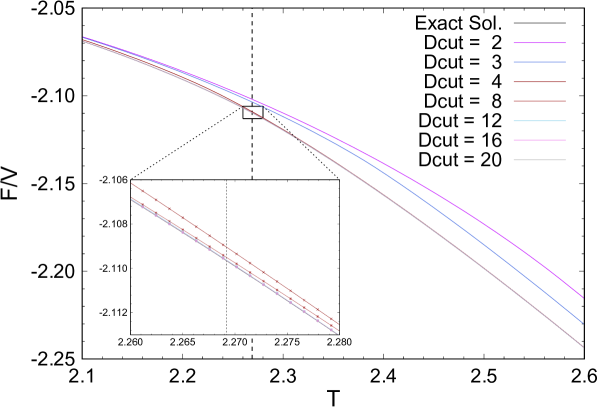
Figure 1: $T$ dependence of free energy density evaluated on $V=2^{16}\times 2^{16}$ lattice.

Figure 2 shows the $D_{\mathrm{cut}}$-dependence of the critical temperature. The numerical results fluctuate around the exact solution $T_{c}^{\rm exact}=2/[\log(1+\sqrt{2})]=2.2691853\cdots$. It is clearly observed that taking the enlarged value of $D_{\mathrm{cut}}$ makes the results approach the exact one.

Figure 2: Critical temperature evaluated on $V=2^{10}\times 2^{10}$ lattice. The computational results are presented as black points, and a dotted line denotes the exact value of the critical temperature $T_{\mathrm{c}}^{exact}=2/[\log(1+\sqrt{2})]=2.2691853\cdots$.

III Irregular parameter dependence of TRG and new scheme with smooth cut

III.1 Origin of irregular behavior

The numerical results of TRG often show the irregular behavior as the parameters are varied. Here we consider the reason why the numerical results do not smoothly depend on the parameters. For simplicity, the numerical computations are performed on $V=(16)^{2}$ in this section.

Figure 3 shows the relative residue of the free energy, which is given by a relative difference between the results of TRG and the exact solution. The irregular behavior is observed as the abrupt jump of the results at several temperatures off the critical point denoted by the black dotted line. For instance, as magnified in the small figure, the result with $D_{\mathrm{cut}}=12$ shows an irregular jump at $T_{\rm ref}\approx 2.6075$.

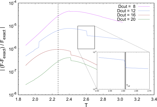
Figure 3: $T$-dependence of the relative residual of the Helmholtz free energy, which is evaluated for $D_{\mathrm{cut}}=8,12,16,20$ on $V=(16)^{2}$ lattice. The gray band in an enlarged figure at the bottom right denotes the region where the irregular behavior is caused.

To understand the origin of this behavior, we write the R.H.S. of Eq. (4) as a form,

$$T^{(1)}_{IJ}=\sum_{m=1}^{D_{\mathrm{cut}}}\lambda_{m}{u}^{(m)}_{I}{v}^{(m)}_{J},$$ (8)

where $\vec{u}^{(m)}$ ($\vec{v}^{(m)}$) is the left (right) singular vector corresponding to the $m$-th singular value $\lambda_{m}$. $T^{(1)}_{IJ}$ is an approximation of the tensor $T_{ijkl}$ for $I=(i,j)$ and $J=(i,j)$. We assume that a set of singular values and corresponding singular vectors $(\lambda,\vec{u}(\lambda),\vec{v}(\lambda))$ smoothly change under a local variation of parameters.

We now consider a case in which the level crossing takes place such that $K$-th and $(K+1)$-th singular values are interchanged at some value of the parameter. The crossover is not important in the case of $K\neq D_{\mathrm{cut}}$ because both of $K$-th and $(K+1)$-th singular values are included (or not included) in Eq. (8). In the case of $K=D_{\mathrm{cut}}$, however, the crossover could make Eq. (8) change drastically: the $D_{\mathrm{cut}}$-th singular vector before the crossover becomes the $(D_{\mathrm{cut}}+1)$-th one after the crossover and vice versa, while the $D_{\mathrm{cut}}$-th singular value changes continuously.

In Fig. 4 we trace the continuous move of the $D_{\mathrm{cut}}$-th and $(D_{\mathrm{cut}}+1)$-th singular values around $T_{\rm ref}$ (gray band), where the $D_{\mathrm{cut}}$-th singular value (open circle) and the $(D_{\mathrm{cut}}+1)$-th singular value (solid circle) are interchanged. Those singular values are obtained in the course-grained tensor after six renormalization steps with $D_{\mathrm{cut}}=12$. We should note that the $(D_{\mathrm{cut}}+1)$-th singular value becomes the $D_{\mathrm{cut}}$-th singular value after the level crossing. The purple line is the $D_{\mathrm{cut}}$-th singular value included in Eq. (8), and the green dotted line is the $(D_{\mathrm{cut}}+1)$-th one. This behavior suggests that the discontinuity of the result of the free energy does not come from the singular values in Eq. (8) but from the discontinuous change of the singular vectors.

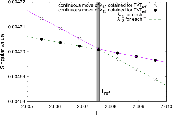
Figure 4: An example of the crossover of the $D_{\mathrm{cut}}$-th and $(D_{\mathrm{cut}}+1)$-th singular values, where $D_{\mathrm{cut}}=12$, as a function of $T$. See text for lines and points.

Let us consider the following modification for the approximation of tensor at the final step of SVD:

$$T^{(2)}_{IJ}=\left\{\begin{array}[]{ll}T^{(1)}_{IJ}&\quad{\rm for}\ T<T_{\rm ref},\\ \displaystyle\sum_{m=1}^{D_{\mathrm{cut}}-1}\lambda_{m}{u}^{(m)}_{I}{v}^{(m)}_{J}+\lambda_{D_{\mathrm{cut}}+1}{u}^{(D_{\mathrm{cut}}+1)}_{I}{v}^{(D_{\mathrm{cut}}+1)}_{J}&\quad{\rm for}\ T\geq T_{\rm ref}.\end{array}\right.$$ (11)

The meaning of this approximation is obvious from the definition. $T^{(2)}$ coincides with $T^{(1)}$ before the level crossing. After the level crossing, however, $T^{(2)}$ continues to keep the same sets $(\lambda,\vec{u}(\lambda),\vec{v}(\lambda))$ unlike $T^{(1)}$. If the irregular behavior is caused by the change of the associated singular vectors, it is expected that the jump at $T_{\rm ref}$ should vanish with the use of $T^{(2)}$.

Figure 5 shows the residues obtained from $T^{(2)}$, which are drawn by the blue curve. They smoothly depend on temperature and the jump at $T_{\rm ref}$ has gone. It is also instructive to check the smooth behavior of the green curve, which represent the results in the case that the $(D_{\mathrm{cut}}+1)$-th set is used instead of $D_{\mathrm{cut}}$-th set for $T<T_{\rm ref}$ (and $T^{(1)}$ is used for $T\geq T_{\rm ref}$). We thus conclude that the irregular behavior is caused by the level crossing of the $D_{\mathrm{cut}}$-th and $(D_{\mathrm{cut}}+1)$-th singular values. More specifically speaking, the replacement of the $D_{\mathrm{cut}}$-th singular vector at the crossover point yields the jump of the results.

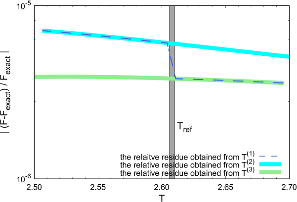
Figure 5: $T$-dependence of the relative residue of the free energy evaluated with $D_{\mathrm{cut}}=12$ on $V=(16)^{2}$ lattice. The blue broken line, the blue and green curves are the relative residue of the free energy obtained from $T^{(1)}$, $T^{(2)}$ and $T^{(3)}$, respectively. $T^{(1)}$ is defined by Eq. (8), and $T^{(1)}$ is defined by Eq. (11). $T^{(3)}$ is the case that the $(D_{\mathrm{cut}}+1)$-th set is used instead of $D_{\mathrm{cut}}$-th set for $T<T_{\mathrm{ref}}$ and $T^{(1)}$ is used for $T\geq T_{\mathrm{ref}}$.

III.2 Test of smooth cutoff schemes

The irregular parameter dependence of the results obtained by the TRG method is caused by the level crossing of the singular values across the truncation order as explained in the previous section. The standard TRG employs the sharp cutoff such that the $D_{\mathrm{cut}}$ largest singular values and the associated vectors are included in the renormalization steps and the others are thrown away. In this section, we test other cutoff scheme such as a smooth cutoff to tame the misbehavior.

In order to define another truncation scheme, we introduce a weight function $w_{m}$ to approximate the tensor $T_{ijkl}$:

$$T_{ijkl}\simeq\sum_{m=1}^{D_{\mathrm{cut}}}w_{m}U_{(ij)m}\lambda_{m}V^{\dagger}_{m(kl)},$$ (12)

where $U$ and $V$ are unitary matrices and $\lambda_{m}$ are singular values sorted in descending order. Note that Eq. (4) is given by the choice of the weight function, $w_{m}=1$ for $m\leq D_{\mathrm{cut}}$. It can be expected that the crossover effect depends on $w_{m}$ and may become weaker if we employ a smoother cutoff function for $w_{m}$. Note that the introduction of $w_{m}$ itself does not demand extra computational cost.

As possible choices of cutoff schemes we consider two types of weight functions: (A) ”a slanting-cut” given by

$$w_{m}^{\rm(A)}=\begin{cases}1&(1\leq m\leq D_{\mathrm{cut}}-\Delta)\\ \frac{D_{\mathrm{cut}}-m}{\Delta}&(D_{\mathrm{cut}}-\Delta<m\leq D_{\mathrm{cut}}),\end{cases}$$ (13)

and (B) ”a FDF-cut” inspired by by the Fermi distribution function

$$w^{\rm(B)}_{m}=\frac{1}{\mathrm{e}^{(m-D_{\mathrm{cut}})/\sigma}+1}.$$ (14)

Figure 6 shows examples of $w_{m}^{\rm(A)}$ and $w_{m}^{\rm(B)}$. $\Delta$ in $w^{\rm(A)}$ and $\sigma$ in $w^{\rm(B)}$ are the tunable parameters which basically give the smeared size of cutoff. In this paper we employ $\Delta=3$ and $\sigma=1$.

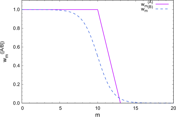
Figure 6: Weight factors $w_{m}^{(\mathrm{A})}$ and $w_{m}^{(\mathrm{B})}$.

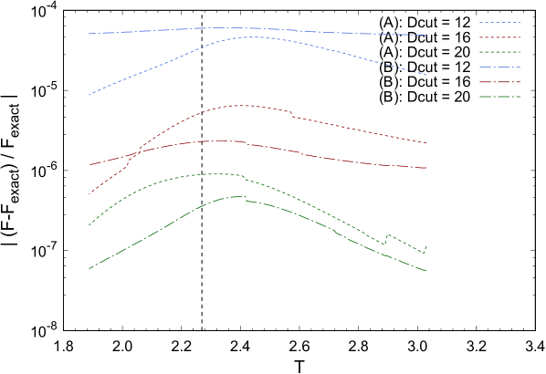
Figure 7: $T$ dependence of the relative residual of the free energy on $V=(16)^{2}$ lattice. The dotted line is for (A) the slanting-cut method with $\Delta=3$ in Eq. (13), and the chain line is for (B) the FDF-cut method with $\sigma=1.0$ in Eq. (14).

Figure 7 shows the relative residues obtained by these two cutoffs, which show smoother temperature dependence compared to those in Fig. 3. It is confirmed that the smooth cutoff scheme is effective to tame the irregular parameter dependence found in the sharp cutoff scheme in the standard TRG method.

IV Summary

We have discussed the issue of the irregular parameter dependence observed in the TRG results. We have investigated its origin using the two-dimensional Ising model and concluded that the irregular behaviors is caused by the level crossing between the singular values in the sharp cutoff scheme with $D_{\mathrm{cut}}$. When the level crossing occurs between the $D_{\mathrm{cut}}$-th and $(D_{\mathrm{cut}}+1)$-th singular values, $D_{\mathrm{cut}}$-th singular vector is replaced by the completely different one across the crossover point, though the $D_{\mathrm{cut}}$-th singular value changes continuously as a function of the parameter. Thus the constructed tensor drastically changes and yields the jump of the numerical result at the crossover point.

We have shown that the smooth cutoff improves the irregular behavior of the free energy in two-dimensional Ising model. Further improvements would be important to obtain the precise results in more complicated lattice models or higher dimensional models with the tensor network schemes.

References

- [1] Michael Levin and Cody P. Nave. Tensor renormalization group approach to 2D classical lattice models. Phys. Rev. Lett., 99(12):120601, 2007.
- [2] Yuya Shimizu. Analysis of the -dimensional lattice model using the tensor renormalization group. Chin. J. Phys., 50:749, 2012.
- [3] Yuya Shimizu and Yoshinobu Kuramashi. Grassmann tensor renormalization group approach to one-flavor lattice Schwinger model. Phys. Rev., D90(1):014508, 2014.
- [4] Judah Unmuth-Yockey, Yannick Meurice, James Osborn, and Haiyuan Zou. Tensor renormalization group study of the 2d O(3) model. 2014.
- [5] Yuya Shimizu and Yoshinobu Kuramashi. Critical behavior of the lattice Schwinger model with a topological term at using the Grassmann tensor renormalization group. Phys. Rev., D90(7):074503, 2014.
- [6] Shinji Takeda and Yusuke Yoshimura. Grassmann tensor renormalization group for the one-flavor lattice Gross-Neveu model with finite chemical potential. PTEP, 2015(4):043B01, 2015.
- [7] Hikaru Kawauchi and Shinji Takeda. Tensor renormalization group analysis of CP(N-1) model. Phys. Rev., D93(11):114503, 2016.
- [8] Y. Meurice, A. Bazavov, Shan-Wen Tsai, J. Unmuth-Yockey, Li-Ping Yang, and Jin Zhang. Tensor RG calculations and quantum simulations near criticality. PoS, LATTICE2016:325, 2016.
- [9] Ryo Sakai, Shinji Takeda, and Yusuke Yoshimura. Higher order tensor renormalization group for relativistic fermion systems. PTEP, 2017(6):063B07, 2017.
- [10] Yusuke Yoshimura, Yoshinobu Kuramashi, Yoshifumi Nakamura, Shinji Takeda, and Ryo Sakai. Calculation of fermionic Green functions with Grassmann higher-order tensor renormalization group. Phys. Rev., D97(5):054511, 2018.
- [11] Yuya Shimizu and Yoshinobu Kuramashi. Berezinskii-Kosterlitz-Thouless transition in lattice Schwinger model with one flavor of Wilson fermion. Phys. Rev., D97(3):034502, 2018.
- [12] Yoshinobu Kuramashi and Yusuke Yoshimura. Three-dimensional finite temperature Z2 gauge theory with tensor network scheme. 2018.
- [13] Daisuke Kadoh, Yoshinobu Kuramashi, Yoshifumi Nakamura, Ryo Sakai, Shinji Takeda, and Yusuke Yoshimura. Tensor network formulation for two-dimensional lattice = 1 Wess-Zumino model. JHEP, 03:141, 2018.
- [14] Lars Onsager. Crystal statistics. i. a two-dimensional model with an order-disorder transition. Phys. Rev., 65:117–149, Feb 1944.
- [15] Bruria Kaufman. Crystal statistics. ii. partition function evaluated by spinor analysis. Phys. Rev., 76:1232–1243, Oct 1949.