Maximum Likelihood Estimation and Graph Matching in Errorfully Observed Networks

Abstract

Given a pair of graphs with the same number of vertices, the inexact graph matching problem consists in finding a correspondence between the vertices of these graphs that minimizes the total number of induced edge disagreements. We study this problem from a statistical framework in which one of the graphs is an errorfully observed copy of the other. We introduce a corrupting channel model, and show that in this model framework, the solution to the graph matching problem is a maximum likelihood estimator (MLE). Necessary and sufficient conditions for consistency of this MLE are presented, as well as a relaxed notion of consistency in which a negligible fraction of the vertices need not be matched correctly. The results are used to study matchability in several families of random graphs, including edge independent models, random regular graphs and small-world networks. We also use these results to introduce measures of matching feasibility, and experimentally validate the results on simulated and real-world networks.

Keywords: Graph matchability, corrupting channel, consistency

1 Introduction

Graphs are a popular data structure used to represent relationships between objects or agents, with successful applications in many different fields, including finance, neuroscience, biology, and sociology, among others. Many applications deal with multiple graph observations that can come as different instances of the graph for the same or related set of vertices, and thus studying these data jointly usually requires knowledge of the correspondence between the vertices first. When this correspondence is unknown or observed with errors, graph matching can be used to first recover the true correspondence before performing subsequent inference. Simply stated, the graph matching problem consists in finding an alignment between the vertices of two different graphs that minimizes a measure of dissimilarity between them (usually specified to be the number of edge differences). This problem has found many useful applications in different areas including de-anonymizing social networks (Narayanan and Shmatikov, 2009; Korula and Lattanzi, 2014; Zhang and Tong, 2016; Heimann et al., 2018), aligning biological networks (Yang and Sze, 2007; Zaslavskiy et al., 2009; Vogelstein et al., 2014), and unsupervised word translation (Grave et al., 2018), among others; see the surveys Conte et al. (2004); Foggia et al. (2014); Yan et al. (2016) for a review (up to 2016) of the graph matching literature and applications.

1.1 The graph matching problem

Formally, given a pair of adjacency matrices for some graphs $A=(E_{1},V_{1})$ and $B=(E_{2},V_{2})$ with equal number of vertices $|V_{1}|=|V_{2}|$ (where $|V|$ denotes cardinality of a set of vertices $V$), the graph matching problem (GMP) consists of finding a mapping $\pi:V_{1}\rightarrow V_{2}$ which aligns the vertices between the two graphs to make the structure most similar; i.e., if $\Pi_{n}$ is the set of $n\times n$ permutation matrices, then the GMP is $\operatorname*{arg\,min}_{P\in\Pi_{n}}\|A-PBP^{T}\|_{F}$, where $\|E\|_{F}=(\sum_{i=1}^{n}\sum_{j=1}^{n}E^{2}_{ij})^{1/2}$ is the Frobenius norm of some matrix $E\in\mathbb{R}^{n\times n}$. Variants of this basic formulation have been proposed in the literature to accommodate more nuanced graph structure including, incorporating weighted and directed edges, $|V_{1}|\neq|V_{2}|$ (Fishkind et al., 2019), vertex and edge covariates (Lyzinski et al., 2016b), and matching multiple graphs simultaneously (Yan et al., 2013).

A special case of the problem is exact graph matching, also known as the graph isomorphism problem (Babai, 2015), where the goal is to determine if there exists an alignment between the vertices of the graphs yielding identical edge structure across networks. Even for this special case, it is currently not known whether the problem is solvable in polynomial time. However, an exact unique solution exists as long as there is no non-identity automorphisms (i.e., $\forall P\neq I_{n}$, $A\neq PAP^{T}$) . In practice, the applicability of exact graph matching is limited due to the fact that data often consists of noisy observations of a graph, and thus one can only hope to recover an alignment that preserves a significant portion of the structure.

In the inexact version of the graph matching problem, a pair of graphs with the same number of vertices is observed, and the goal is to find an alignment of the vertices that best preserves the structure of the graphs. This is often accomplished by minimizing an appropriate dissimilarity measure over all the possible permutations (e.g., the Frobenius norm formulation considered above). Several random graph models have been proposed in the recent literature, and these have been used to study the difficulty and feasibility of this problem. These models often parametrically enforce a natural similarity between the graphs while still allowing for structural differences. They vary in complexity from correlated homogeneous Erdős-Rényi networks (Pedarsani and Grossglauser, 2011; Yartseva and Grossglauser, 2013; Lyzinski et al., 2014b), to correlated stochastic blockmodel networks (Onaran et al., 2016; Lyzinski and Sussman, 2020), to correlated general edge independent networks (Korula and Lattanzi, 2014; Lyzinski et al., 2016a), to independent graphon generated networks (Zhang, 2018b). Within these models, the dual problems of developing efficient graph matching algorithms and studying the theoretical feasibility of the GMP have been considered. However, beyond (conditionally) edge-independent networks, few theoretical guarantees exist for either algorithmic performance (see Korula and Lattanzi (2014) for an example of matching guarantees in a preferential attachment model).

1.2 Graph matchability and maximum likelihood estimation

These random graph models have allowed for the exploration of the related notion of graph matchability: given a natural correspondence between the vertex sets of two networks, can the GMP uncover this correspondence in some statistical sense (Lyzinski et al., 2014b, 2016a; Lyzinski, 2018; Onaran et al., 2016; Cullina and Kiyavash, 2017)? In this paper, we cast the problem of graph matchability in the framework of maximum likelihood (ML) estimation, equating matchability with the consistency of the maximum likelihood estimator (MLE) of an unknown correspondence. The results bear a similar flavor to those in Onaran et al. (2016) (and Cullina and Kiyavash (2016)), wherein a model for correlated stochastic blockmodels is proposed. In their framework, they showed that maximum a posteriori (MAP) estimation is the same as optimizing a weighted variant of the classical graph matching problem. Unlike previous work, our model (see Section 2.1) is designed to be distribution-free, allowing for corrupted or correlated observations of arbitrarily structured networks to be considered. We note that while we are not the first to frame the GMP as a ML estimation problem (see, for example, Luo and Hancock (2001); Lyzinski et al. (2016b)), our model allows for a novel understanding of the relationship between the two, seemingly disparate, ideologies.

While maximum likelihood estimation is a core concept in modern statistical inference (Stigler, 2007), estimation of an unknown correspondence between two networks presents the challenge of ML estimation in the presence of a growing parameter dimension. Our model is parameterized by the shuffling permutation, which is the parameter of interest, and corrupting probabilities for each edge that are nuisance parameters. Indeed, viewing the correspondence between vertices as a parameter to be estimated, this parameter naturally contains $n-1$ free variables, where $n$ is the number of vertices in the observed network, while the number of nuisance parameters can grow as $O(n^{2})$. Asymptotics (as $n\rightarrow\infty$, yielding $\binom{n}{2}$ sample size) resist the classical theoretical framework when the number of (nuisance) parameters grow with the sample size (see, for example, Bickel and Doksum (2015)), and the MLE can be inconsistent in this setting (Neyman and Scott, 1948; Lancaster, 2000). Recently, statistical network inference (see, for example, Bickel and Chen (2009); Zhao et al. (2012)) has presented further examples of consistent ML estimation in networks when the parameter dimension is growing, notably for the inference task of community detection in stochastic blockmodel random graphs. By equating consistent ML estimation with graph matchability, we provide another class of examples in the network literature for which consistency of the MLE is achieved as the graph size (and parameter dimension) increases.

The paper is organized as follows. In Section 2.1 we introduce the corrupting channel model and show that maximum likelihood estimation of the latent vertex correspondence is a solution to the graph matching problem (and vice versa). Next, in Section 3 we derive necessary and sufficient conditions (depend on the structure of the given graph and the channel noise) for consistency of the MLE. In Section 4 we introduce a notion of quasi-consistency in which we allow a fraction of the vertices to be incorrectly matched, and present sufficient conditions to achieve this property. Results of consistency and quasi-consistency of the MLE in a variety of random graph models are presented, including some new results for small-world and random regular graphs. In Section 5 we introduce a practical approach to studying matchability, and validate our theoretical results with numerical experiments on simulated networks from popular random graph models and real-world data from different domains. We conclude with a discussion and remarks in Section 6.

2 Equivalence between maximum likelihood estimation and graph matching

2.1 Uniformly corrupting channel

Consider the set of undirected graphs with no self-loops and $n$ labeled vertices, which we denote by $\mathcal{G}_{n}$. Each graph will be represented with an adjacency matrix $A\in\{0,1\}^{n\times n}$, which is symmetric and hollow (i.e., with zeros in the diagonal). Let $p\in[0,1]$, $P\in\Pi_{n}=\{n\times n\text{ permutation matrices}\}$, and $A\in\mathcal{G}_{n}$. We model passing $A$ through an edge and vertex-label corrupting channel as follows.

Definition 1.

Define the graph-valued random variable $B_{p,P}$ (i.e., the channel-corrupted $A$) parameterized by $(p,P)$ via $B_{p,P}:=P(X\circ(1-A)+(1-X)\circ A)P^{T}$, where $X\in\mathbb{R}^{n\times n}$ is a symmetric, hollow matrix with i.i.d. $\text{Bernoulli}(p)$ entries in its upper triangular part, $X$ is independent of $A$, and $``\circ"$ is the Hadamard matrix product. For ease of notation, we shall write $B_{p,P}=B\sim$C$(A,p,P)$ for $B$ distributed as the channel corrupted $A$.

Note that if $A$ is a graph-valued random variable, then we further assume that $X$ is independent of $A$. This model is similar to the noisily observed network models of Pedarsani and Grossglauser (2011); Yartseva and Grossglauser (2013); Korula and Lattanzi (2014); Chang et al. (2018). Note that here we make no assumptions on the distribution of the underlying graph $A$; indeed, below we often view $A$ as deterministic and not random, and consider the distribution of $B$ conditional on $A$.

Stated simply, $B_{p,P}$ is formed by first uniformly corrupting (i.e., bit-flipping) edges in $A$ independently with probability $p$ and then shuffling the labels via $P$. Given observed $(A,B)$, the likelihood of $(p,P)$ in this model is given by

$$L(p,P)=\prod_{i<j}(1-p)^{\mathds{1}\{A_{i,j}=(P^{T}BP)_{i,j}\}}p^{\mathds{1}\{A_{i,j}\neq(P^{T}BP)_{i,j}\}},$$

so that the log-likelihood is given by

$$\ell(p,P) =\sum_{i<j}\mathds{1}\{A_{i,j}=(P^{T}BP)_{i,j}\}\log(1-p)+\mathds{1}\{A_{i,j}\neq(P^{T}BP)_{i,j}\}\log p$$

$$=\frac{1}{2}\text{tr}(AP^{T}BP)\log(1-p)+\frac{1}{2}\left(n(n-1)-\text{tr}(AP^{T}BP)\log p\right)$$

$$=\frac{1}{2}\text{tr}(AP^{T}BP)(\log(1-p)-\log p)+\frac{n(n-1)\log p}{2},$$

and given a fixed value of $p$, observing that $2\text{tr}(AP^{T}BP)=\|A\|_{F}^{2}+\|B\|_{F}^{2}-\|A-P^{T}BP\|_{F}^{2}$, the (possibly non-unique) MLE of $P$ is then given by

$$\hat{P}_{\text{MLE}}=\begin{cases}\text{any }P\in\operatorname*{arg\,min}_{P\in\Pi_{n}}\|A-P^{T}BP\|_{F}^{2}&\text{ for }p<1/2\\ \text{any }P\in\text{argmin}_{P\in\Pi_{n}}\|A-P^{T}\breve{B}P\|_{F}^{2}&\text{ for }p>1/2\\ \text{any }P\in\Pi_{n}&\text{ for }p=1/2,\end{cases}$$

where $\breve{B}$ is the complement of the graph $B$ (i.e., $\breve{B}_{ij}=1-B_{ij}$). In the $p<1/2$ setting, the problem of maximum likelihood estimation is equivalent to the problem of graph matching, as the classical GMP formulation is to find the (possibly non-unique) minimizer of a quadratic assignment problem (QAP) of the form

$$\hat{P}_{\text{GM}}\in\operatorname*{arg\,min}_{P\in\Pi_{n}}\|A-P^{T}BP\|_{F}^{2}$$ (1)

Analogously, when $p>1/2$, ML estimation is equivalent to matching one graph with the complement of the other.

A natural first question to ask is what properties $A$ (and $p$) must possess in order for the MLE for $P$ to be consistent, and hence the vertex-label corruption introduced into $B$ can be undone via graph matching. We note here that the parameter dimension of $P$ is growing in $n$ and classical ML estimation consistency results do not directly apply (see, for example, Bickel and Doksum (2015)). Nonetheless, in Section 3 our main result, Theorem 4, will establish consistency of the MLE under fairly modest assumptions on $A$ and $p$.

2.2 Heterogeneous corrupting channel

The uniform corrupting channel model defined above assumes that all edges of $A$ are corrupted with the same probability. However, in some cases it is more reasonable to consider a model in which each pair of vertices might be corrupted with different probabilities. For example, we can consider the setting in which edges and non-edges in $A$ are corrupted by the channel independently with different probabilities, or in which certain vertices or edges are more likely to be corrupted. Thus, we also consider an heterogeneous corrupting channel defined as follows.

Definition 2.

Let $\Psi^{(m)}\in[0,1]^{n\times n},m=1,2$ be two matrices that correspond to the corrupting probabilities for edges and non-edges, and $P\in\Pi_{n}$. For a given adjacency matrix $A\in\{0,1\}^{n\times n}$, we define $B_{\Psi^{(1)},\Psi^{(2)},P}$ as

$$B_{\Psi^{(1)},\Psi^{(2)},P}=P(X\circ(1-A)+(1-Y)\circ A)P^{T},$$

where $X$ and $Y$ are symmetric hollow matrices such that $X_{ij}\sim\text{Bernoulli}(\Psi^{(1)}_{ij})$ and $Y_{ij}\sim\text{Bernoulli}(\Psi^{(2)}_{ij})$ and $\{X_{i,j},Y_{i,j}\}_{i<j}$ are independent. Dropping subscripts to ease notation when possible, we denote it via $B\sim\text{C}(A,\Psi^{(1)},\Psi^{(2)},P)$ for $B$ distributed as the heterogeneous corrupting channel $A$.

Note that if $A$ is a graph-valued random variable, then we further assume that $X$ and $Y$ are independent of $A$. The heterogeneous corrupting channel model is saturated, but the only parameter of interest is $P$.

The flexibility of having different corrupting probabilities for each edge allows us to include other popular graph models within this framework. In particular, if $A\sim\text{Bernoulli}(\Lambda)$, the heterogeneous corrupting channel model can be used to describe the distribution of a pair of correlated Bernoulli graphs conditional on the first graph. In more detail, given a pair of hollow symmetric matrices $R,\Lambda\in[0,1]^{n\times n}$, the pair of graphs $A,B$ is said to be distributed as $R$-correlated random Bernoulli$(\Lambda)$ graphs if marginally $A,B\sim\text{Bernoulli}(\Lambda)$ (i.e., for $1\leq i<j\leq n$, $A_{ij}$ are independently distributed as $\text{Bern}(\Lambda_{ij})$ random variables; similarly for $B$) and each pair of variables $A_{ij},B_{\ell k}$, $1\leq i<j\leq n,1\leq\ell<k\leq n$, $(i,j)\neq(\ell,k)$ are mutual independent, except that for each $1\leq i<j\leq n$, $\text{corr}(A_{ij},B_{ij})=R_{ij}$. Note that in the correlated Bernoulli graphs model, $\mathbb{P}(B_{ij}=1|A_{ij})=A_{ij}R_{ij}+(1-R_{ij})\Lambda_{ij}$, so the distribution of $B$ conditioned on $A$ can be written using an heterogeneous channel with

$$\Psi^{(1)}_{ij} = (1-R_{ij})\Lambda_{ij}$$ (2)

$$\Psi^{(2)}_{ij} = (1-R_{ij})(1-\Lambda_{ij}).$$ (3)

This correlated Bernoulli graph model, and in particular, the correlated Erdős-Rényi (ER) model (in which each of the matrices $\Lambda$ and $R$ have the same value in all the entries), have been extensively used in studying the inexact graph matching problem (Pedarsani and Grossglauser, 2011; Lyzinski et al., 2014a, 2016a; Cullina and Kiyavash, 2017; Ding et al., 2018; Mossel and Xu, 2019). The corrupting channel model is thus comprehensive enough to include other popular settings in literature (see for example Corollary 6 for a result in correlated ER graphs), while allowing to extend some of the results to graphs with arbitrary structure.

In the heterogeneous corrupting channel, the MLE of the unshuffling permutation is also exactly equivalent to the minimizer of the graph matching objective (1). Note that in this case, the likelihood is given by

$$\ell(\Psi^{(1)},\Psi^{(2)},P) = \sum_{i<j}\left\{(P^{T}{B}P)_{ij}\log\left((1-\Psi^{(1)}_{ij})A_{ij}+\Psi^{(2)}_{ij}(1-A_{ij})\right)\right.$$

$$\left.+(1-(P^{T}{B}P)_{ij})\log\left(\Psi^{(1)}_{ij}A_{ij}+(1-\Psi^{(2)}_{ij})(1-A_{ij})\right)\right\}.$$

In general, the MLE for $P$ in this model is not unique since the corrupting probabilities can arbitrarily alter the graph. Thus, we impose a further assumption that the probability of any pair of corresponding edges in the graphs $A$ and $B$ to be the same is at least 0.5. Formally, let $\tilde{p}=\max_{i,j,k}\Psi^{(k)}_{ij}$ be the largest corrupting probability for an edge. Under the assumption that $\tilde{p}\leq\frac{1}{2}$, for a given $P\in\Pi_{n}$ we can calculate a profile MLE for $\Psi^{(k)},k=1,2$, denoted by $\hat{\Psi}^{(k)}(P)$, as

$$\left(\hat{\Psi}^{(k)}(P)\right)_{ij}=\begin{cases}0&\text{if $A_{ij}=(P^{T}{B}P)_{ij},$}\\ \frac{1}{2}&\text{if $A_{ij}\neq(P^{T}{B}P)_{ij}$}\end{cases}.$$ (4)

Thus, the profile loglikelihood for $P$ can be expressed as

$$\ell\left(\!\hat{\Psi}^{(1)}(P),\hat{\Psi}^{(2)}(P),P\!\right) =\sum_{i<j}2\mathds{1}(A_{ij}\neq(P^{T}{B}P)_{ij})\log(1/2)$$

$$=-\log(2)\|A-(P^{T}{B}P)\|_{F}^{2},$$

which does not depend on the particular values of $\hat{\Psi}^{(1)}(P),\hat{\Psi}^{(2)}(P)$ and is proportional to the graph matching objective (1). Therefore, the (possibly non-unique) MLE for $P$, given by

$$\hat{P}_{\text{MLE}}\in\operatorname*{arg\,max}_{P\in\Pi_{n}}\ell\left(\!\hat{\Psi}^{(1)}(P),\hat{\Psi}^{(2)}(P),P\!\right)$$

is exactly equivalent to the solution of the GMP.

3 Consistency of the maximum likelihood estimator

For a given positive integer $n_{0}$, consider a sequence of graphs $(A_{n})_{n=n_{0}}^{\infty}$ (with the order of $A_{n}$ being $n$). For the parameter sequence $(\,(p_{n},P_{n})\,)_{n=n_{0}}^{\infty}$, consider the sequence of channel-corrupted $A_{n}$’s defined via

$$\left(B_{n}=P_{n}(X_{n}\circ(1-A_{n})+(1-X_{n})\circ A_{n})P_{n}^{T}\right)_{n=n_{0}}^{\infty},$$

where each $X_{n}$ is a symmetric, hollow matrix with i.i.d. $\text{Bernoulli}(p_{n})$ entries in its upper triangular part, and the $X_{n}$’s are mutually independent across index $n$. In this setting, we define consistency of a sequence of estimators as follows.

Definition 3 (Consistency).

With $(B_{n}\sim\text{C}(A_{n},p_{n},P_{n}))_{n=n_{0}}^{\infty}$ defined as above, for $n\geq n_{0}$ we say that a sequence of estimators $(\hat{P}_{n}:=\hat{P}_{n}(A_{n},B_{n}))_{n=n_{0}}^{\infty}$ of $(P_{n})_{n=n_{0}}^{\infty}$, is a $\begin{pmatrix}\text{weakly}\\ \text{strongly}\end{pmatrix}$ consistent estimator if $\|\hat{P}_{n}-P_{n}\|_{F}\begin{pmatrix}\stackrel{{\scriptstyle P}}{{\rightarrow}}\\ \stackrel{{\scriptstyle a.s.}}{{\rightarrow}}\end{pmatrix}0$ as $n\rightarrow\infty$, for all sequences $(P_{n})_{n=n_{0}}^{\infty}$.

As the MLE of $(P_{n})_{n=n_{0}}^{\infty}$ is not necessarily uniquely defined (i.e., there are multiple possible MLEs for a given $n$), we write that the MLE of $(P_{n})_{n=n_{0}}^{\infty}$ is $\begin{pmatrix}\text{weakly}\\ \text{strongly}\end{pmatrix}$ consistent if $\max_{Q_{n}\in\mathcal{P}^{*}_{n}}\|Q_{n}-P_{n}\|_{F}\begin{pmatrix}\stackrel{{\scriptstyle P}}{{\rightarrow}}\\ \stackrel{{\scriptstyle a.s.}}{{\rightarrow}}\end{pmatrix}0$ as $n\rightarrow\infty$, where

$$\mathcal{P}^{*}_{n}=\operatorname*{arg\,min}_{P\in\Pi_{n}}\|A_{n}-P^{T}B_{n}P\|^{2}_{F}.$$

Note that, as $\max_{Q_{n}\in\mathcal{P}^{*}_{n}}\|Q_{n}-P_{n}\|^{2}_{F}$ is integer-valued, strong consistency of the MLE is equivalent to

$$\mathbb{P}(\max_{Q_{n}\in\mathcal{P}^{*}_{n}}\|Q_{n}-P_{n}\|^{2}_{F}=0\text{ for all but finitely many }n)=1$$

$$\Longleftrightarrow\mathbb{P}(\mathcal{P}^{*}_{n}=\{P_{n}\}\text{ for all but finitely many }n)=1.$$

Loosely speaking, a estimator is consistent if the number of vertices that are incorrectly matched by the estimator goes to zero as the size of the graph increases. It is clear that consistency of an estimator hinges on the properties of $(A_{n})_{n=n_{0}}^{\infty}$. Indeed, if infinitely many $A_{n}$ have a non-trivial automorphism group, so that there is at least one $Q_{n}\in\Pi_{n}$ such that $Q_{n}\neq I_{n}$ but $A_{n}=Q_{n}^{T}A_{n}Q_{n}$, then the MLE has no hope of consistency in the strong or weak sense. In those circumstances, the most we can hope is that the MLE converges to an element within the automorphism group of the graph (see Remark 5). If, on the other hand, the $A_{n}$’s are sufficiently asymmetric (see Theorem 4 below for a precise definition of this) then the MLE will be strongly consistent under mild model assumptions.

Before stating the theorem, recall that two permutation matrices $Q,Q^{\prime}\in\Pi_{n}$ are disjoint if each one permutes different vertices, that is, if $\sigma_{Q},\sigma_{Q^{\prime}}$ are the permutations associated to each matrix, then $\{i\text{ s.t. }\sigma_{Q}(i)\neq i\}\cap\{i\text{ s.t. }\sigma_{Q^{\prime}}(i)\neq i\}=\emptyset.$ The same definition holds for sets of $k$ permutations. To wit we have the following result (the proof is provided in Appendix A.1).

Theorem 4.

Let $n_{0}>0$, and consider a sequence of graphs $(A_{n})_{n=n_{0}}^{\infty}$. Define the sequence $(B_{n}\sim\text{C}(A_{n},p_{n},P_{n}))_{n=n_{0}}^{\infty}$ of channel-corrupted $A_{n}$’s with parameter sequence $(\,(p_{n},P_{n})\,)_{n=n_{0}}^{\infty}$ and $p_{n}<1/2$.

• For each $n\geq n_{0}$ and each $k\in[n]$, $k\geq 2$, let $\Pi_{n,k}$ be the set of permutation matrices in $\Pi_{n}$ permuting precisely $k$ labels. If there exists an $n_{1}\geq n_{0}$ such that for all $n\geq n_{1}$ and $k\in[n]$,

  $$\min_{Q\in\Pi_{n,k}}\|A_{n}-Q^{T}A_{n}Q\|^{2}_{F}>\frac{6k\log(n)}{\log\left(\frac{1}{4p_{n}(1-p_{n})}\right)}\quad\quad\quad\forall k\geq 2,$$ (5)

  then the MLE of $(P_{n})_{n=n_{0}}^{\infty}$ is strongly consistent.

• If for infinitey many $n>n_{0}$ there exists a sequence $(k_{n})$ with $k_{n}=\Theta(1)$ and a set of disjoint permutations $S_{n}\subset(\cup_{i=2}^{k_{n}}\Pi_{n,i})\setminus\{P_{n}\}$ with $|S_{n}|=\Theta(n)$ , such that

  $$\min_{Q_{n}\in S_{n}}\log\left(\frac{1}{4p_{n}(1-p_{n})}\right)\left(\|A_{n}-Q_{n}^{T}A_{n}Q_{n}\|^{2}_{F}\right)=\omega(1)$$ (6)

  $$\max_{Q_{n}\in S_{n}}\log\left(\frac{1}{4p_{n}(1-p_{n})}\right)\frac{\|A_{n}-Q_{n}^{T}A_{n}Q_{n}\|^{2}_{F}}{\log\|A_{n}-Q_{n}^{T}A_{n}Q_{n}\|^{2}_{F}}=o(1)$$ (7)

  then the MLE of $(P_{n})_{n=n_{0}}^{\infty}$ is not weakly consistent.

• If for infinitely many $n\geq n_{0}$, there exists $Q_{n}\in\Pi_{n}\setminus\{P_{n}\}$ such that

  $$\log\left(\frac{1}{4p_{n}(1-p_{n})}\right)\|A_{n}-Q_{n}^{T}A_{n}Q_{n}\|^{2}_{F}=O\left(1\right),$$ (8)

  then the MLE of $(P_{n})_{n=n_{0}}^{\infty}$ is not weakly consistent.

The previous theorem presents necessary and sufficient conditions in the sequence of graphs $(A_{n})$ to determine whether the MLE for the unshuffling permutation is consistent. Equation (5) quantifies how different $A_{n}$ needs to be from any shuffled version $Q^{T}A_{n}Q$ so that the minimizer of the GMP matches the vertices correctly in the limit. Although verifying this condition for a given graph is computationally hard, it can be shown to hold with high probability via a union bound in some popular random graph models, including the Erdős-Rényi model (see Corollaries 6, 7 and 8). Note that for a given sequence of graphs $(A_{n})_{n=1}^{\infty}$, Equation (5) implies that any sequence of corrupting probabilities $(p_{n})$ such that

$$p_{n}\leq\min_{k\in[n]}\left\{p_{n,k}^{\ast}:=\min_{Q\in\Pi_{n,k}}\left[\frac{1}{2}-\frac{1}{2}\left(1-\exp\left(-\frac{6k\log n}{\|A_{n}-Q^{T}A_{n}Q\|^{2}_{F}}\right)\right)^{1/2}\right]\right\}.$$ (9)

will ensure that the MLE is strongly consistent. The right hand side of Equation (9) thus quantifies how much noise can be supported by the graph, and hence provides a measure of matching feasibility.

The second and third parts of Theorem 4 provide sufficient conditions for inconsistency of the MLE. If for infinitely many values of $n$ there are enough permutations $Q_{n}\in\Pi_{n}\setminus\{I_{n}\}$ for which $\|A_{n}-Q_{n}^{T}A_{n}Q_{n}\|_{F}^{2}$ is small, then there is a non-negligible probability that $\|A_{n}-Q_{n}^{T}(P_{n}BP_{n}^{T})Q_{n}\|_{F}^{2}\leq\|A_{n}-P_{n}BP_{n}^{T}\|_{F}^{2}$ for some $Q_{n}$, and hence, the MLE is not consistent. The number of permutations required for this to happen depends on how small $\|A_{n}-Q_{n}^{T}A_{n}Q_{n}\|_{F}^{2}$ is, and only one permutation is enough if Equation (8) hold, or $\Theta(n)$ of them with the weaker bound in Equation (7). Note that condition (6) can essentially be dropped since when this condition fails then (9) holds. Conditions (6)–(7) imply that $p_{n}\rightarrow 1/2$ and so $\log\left(1/(4p_{n}(1-p_{n}))\textbf{}\right)=(1+o(1))\left(\frac{1}{2}-p_{n}\right)^{2}$; this fact will be used often in the sequel (for example, in Corollary 8). Finally, for part ii., observe that when $\max_{Q\in S_{n}}\|A_{n}-Q_{n}^{T}A_{n}Q_{n}\|_{F}^{2}=\Omega(n^{\delta})$ for some $\delta>0$, then the rates in Equations (5) and (7) have the same order.

Remark 5.

Denote by $\text{Aut}(A_{n})=\{Q\in\Pi_{n}:Q^{T}AQ=A\}$ the automorphism group of a graph $A_{n}$. As mentioned before, when $\text{Aut}(A_{n})\neq I_{n}$ for infinitely many values of $n$, there is no hope of consistency, but the estimator might still converge to an element within the automorphism group of the graphs so that $\|\hat{P}_{n}^{T}(P_{n}A_{n}P_{n}^{T})\hat{P_{n}}-A\|_{F}^{2}\rightarrow 0$ in some weak or strong sense. In this setting, it is possible to derive a result analogous to Theorem 4 by counting the number of edge disagreements $\|A_{n}-Q^{T}_{n}A_{n}Q_{n}\|_{F}^{2}$ only for the permutations $Q_{n}\in\Pi_{n}\setminus\text{Aut}(A_{n})$. The statement and proof of this result are analogous to Theorem 4.

While the correlation structure between $A$ and $B$ in the above Theorem is different than the $\rho$-correlated Bernoulli model of Lyzinski et al. (2014b); Lyzinski (2018); Lyzinski et al. (2016a), this theorem, in a sense, partially unifies many of the edge-independent matchability results appearing in previous work (Lyzinski et al., 2014b, 2016a; Lyzinski, 2018; Onaran et al., 2016; Cullina and Kiyavash, 2017). To wit, we have the following corollary, whose proof follows immediately from Theorem 4 and results in Lyzinski et al. (2016a) (see Appendix A.2 for proof details).

Corollary 6.

Let $n_{0}>0$, and consider an independent sequence of graphs $(A_{n})_{n=n_{0}}^{\infty}$ where for each $n$, $A_{n}\sim$Bernoulli$(\Lambda_{n})$ with $\alpha_{n}\leq\Lambda_{n}\leq 1-\alpha_{n}$ entry-wise. Define the sequence $(B_{n}\sim\text{C}(A_{n},p_{n},P_{n}))_{n=n_{0}}^{\infty}$ of channel-corrupted $A_{n}$’s with parameter sequence $(\,(p_{n},P_{n})\,)_{n=n_{0}}^{\infty}$ and $p_{n}<1/2$. If $\alpha_{n}\left(\frac{1}{2}-p_{n}\right)=\omega\left(\sqrt{\frac{\log n}{n}}\right),$ then the MLE (obtained by solving the GMP) is strongly consistent.

The Erdős-Renyi model (ER) (Erdős and Rényi, 1963) $\text{G}(n,\alpha)$, $\alpha\in(0,1)$ is a particular example of a Bernoulli graph $\text{Bernoulli}(\Lambda)$ in which all entries of $\Lambda$ are equal to $\alpha$, and hence the result of the previous corollary directly applies. By considering concentration bounds on the number of edges in Erdős-Rényi G$(n,\alpha)$ random graphs (i.e., the number of edges is in $n\alpha\pm\sqrt{n\log n}$ with high probability) and the growth rate of $\alpha_{n}$ in Corollary 6, we arrive at the following corollary for Erdős-Renyi graphs $\text{G}(n,m)$ (i.e., uniformly distributed on the set of graphs with exactly $m\in\mathbb{N}$ edges):

Corollary 7.

Let $n_{0}>0$, and consider an independent sequence of graphs $(A_{n})_{n=n_{0}}^{\infty}$ where for each $n$, $A_{n}\sim$G$(n,m_{n})$. Define the sequence $(B_{n}\sim\text{C}(A_{n},p_{n},P_{n}))_{n=n_{0}}^{\infty}$ of channel-corrupted $A_{n}$’s with $p_{n}<1/2$. If

$$m_{n}\left(\frac{1}{2}-p_{n}\right)=\omega\left(\sqrt{n\log n}\right),$$

then the MLE of $(P_{n})_{n=n_{0}}^{\infty}$ is strongly consistent.

Small-world graph models aim to reproduce the property that in many real networks the clustering coefficient is relatively small and paths between any pair of vertices have a short length, usually of order $\log n$ (Watts and Strogatz, 1998). The Newman-Watts (NW) model (Newman and Watts, 1999)—a more easily analyzed variant of the original Watts-Strogatz model —is one such model that adheres to these properties with high probability. The NW model $\text{NW}(n,d,\beta)$ starts with a $d$-ring lattice $A$ in which each vertex is connected with all neighbors that are at a distance no larger than $d$; that is, $A_{ij}=1$ whenever $0<|i-j|\text{mod}(n-1-d)<d$. To generate a small-world behavior, random edges are added independently with probability $\beta$ between vertices that are not connected in the $d$-ring lattice, so $A_{ij}\sim\text{Bernoulli}(\beta)$ for $|i-j|\ \text{mod}(n-1-d)\geq d$.

In the Newman-Watts model, the average path length when $\beta=0$ is $O(n/d_{n})$, and as $\beta$ increases and more edges are added to the graph, there is a phase transition in which the small-world property appears. The next corollary establishes a similar phenomenon in the matching feasibility context: when $\beta$ is small, the MLE is not weakly consistent for matching a NW graph $A$ with a random copy generated from the corrupting channel model, but once there are enough random edges included, the MLE becomes strongly consistent and hence graph matching is feasible. See Appendix A.3 for the proof details.

Corollary 8.

Let $n_{0}>0$ and consider $(A_{n})_{n=n_{0}}^{\infty}$ an independent sequence of graphs such that $A_{n}\sim NW(n,d_{n},\beta_{n})$. Define $(B_{n})_{n=n_{0}}^{\infty}$ as a sequence of channel corrupted graphs with $B_{n}\sim\text{C}(A_{n},p_{n},P_{n})$ and $p_{n}<1/2$.

1. For any sequence $(d_{n})_{n=n_{0}}^{\infty}$, if $(1/2-p_{n})^{2}=o\left(\sqrt{\log n/n}\right)$ and

   $$\beta_{n}=o\left(\frac{\log n}{(1/2-p_{n})^{2}n}\right),$$ (10)

   then the MLE of $(P_{n})_{n=n_{0}}^{\infty}$ (obtained by solving the GMP (1)) is not weakly consistent.

2. If $d_{n}=o(\beta_{n}^{2}n)$, $\beta_{n}\leq 1/2$ and

   $$\beta_{n}=\omega\left(\sqrt{\frac{\log n}{\left({1}/{2}-p_{n}\right)^{2}n}}\right),$$ (11)

   then the MLE of $(P_{n})_{n=n_{0}}^{\infty}$ is strongly consistent.

Using results on the diameter of Erdős-Renyi graphs (Chung and Lu, 2001), it can be verified that if $\beta_{n}$ satisfies Equation (10) for a fixed value of $p_{n}<1/2$ and $\beta_{n}=\omega(1/n)$, then $\text{diam}(A_{n})=O\left(\frac{\log(n)}{\log(n\beta_{n})}\right)$. Thus, there is a regime for $\beta_{n}$ in which NW graphs are small-world but the MLE is not consistent. However, since $\omega(1)=\log(n\beta_{n})=o(\log\log n)$ in this regime, the diameter of the graph is close to $O(\log n)$ and hence it is not far from the phase transition of small-world graphs. If part b) of Corollary 7 holds, then $\text{diam}(A_{n})=O(1)$, so the average path length in NW graphs with a strongly consistent MLE is much smaller than in small-world graphs.

Corollary 8 also suggests a way of making any given graph $A$, with a sufficiently large number of vertices $n$, matchable with a graph corrupted with probability $p$. By setting $\beta=\sqrt{\log(n)/((1/2-p)^{2}n)}$ as in Equation (11) and generating a graph $A^{\prime}\sim\text{C}(A,\beta,I)$, the solution of the graph matching problem between $A^{\prime}$ and $B$ will correctly align all of the vertices with high probability. This result can have applications in settings such as network anonymization (Narayanan and Shmatikov, 2009) and differential privacy (Dwork and Roth, 2014), among others.

3.1 Consistency on the heterogeneous corrupting channel

We now present a more general version of Theorem 4 for the heterogeneous corrupting channel introduced in Section 2.2. In the heterogeneous model, $\Psi^{(1)}$ and $\Psi^{(2)}$ are nuisance parameters when estimating the permutation parameter $P$, so the number of nuisance parameters is $n(n-1)$, which scales with the sample size. Moreover, as can be observed from Equation (4), the MLE of these parameters is not consistent. In this setting, one should be careful when using the MLE for $P$ since this estimator can be inconsistent as shown in the famous Neyman-Scott paradox (Neyman and Scott, 1948). Fortunately, this is not the case here and the MLE can consistently estimate $P$. See Section A.1 for the proof of this Theorem.

Theorem 9.

Let $n_{0}>0$, and consider a sequence of graphs $(A_{n})_{n=n_{0}}^{\infty}$. Define the sequence $(B_{n}\sim\text{C}(A_{n},\Psi^{(1)}_{n},\Psi^{(2)}_{n},P_{n}))_{n=n_{0}}^{\infty}$ of channel-corrupted $A_{n}$’s with parameter sequence $(\,(\Psi_{n}^{(1)},\Psi_{n}^{(2)},P_{n})\,)_{n=n_{0}}^{\infty}$ and $\tilde{p}_{n}:=\max_{i,j,k}(\Psi^{(k)}_{n})_{ij}<1/2$, $\breve{p}_{n}=\min_{i,j,k}(\Psi^{(k)}_{n})_{ij}\geq 0$.

• For each $n\geq n_{0}$ and each $k\in[n]$, $k\geq 2$, let $\Pi_{n,k}$ be the set of permutation matrices in $\Pi_{n}$ permuting precisely $k$ labels. If there exists an $n_{1}\geq n_{0}$ such that for all $n\geq n_{1}$ and $k\in[n]$,

  $$\min_{Q\in\Pi_{n,k}}\|A_{n}-Q^{T}A_{n}Q\|^{2}_{F}>\frac{6k\log(n)}{\log\left(\frac{1}{4\tilde{p}_{n}(1-\tilde{p}_{n})}\right)}\quad\quad\quad\forall k\geq 2,$$ (12)

  then the MLE of $(P_{n})_{n=n_{0}}^{\infty}$ is strongly consistent.

• If for infinitely many $n>n_{0}$ there exists a sequence $(k_{n})$ with $k_{n}=\Theta(1)$ and a set of disjoint permutations $S_{n}\subset(\cup_{i=2}^{k_{n}}\Pi_{n,i})\setminus\{P_{n}\}$ with $|S_{n}|=\Theta(n)$, such that

  $$\min_{Q_{n}\in S_{n}}\log\left(\frac{1}{4\tilde{p}_{n}(1-\tilde{p}_{n})}\right)\left(\|A_{n}-Q_{n}^{T}A_{n}Q_{n}\|^{2}_{F}\right)=\omega(1)$$ (13)

  $$\max_{Q_{n}\in S_{n}}\log\left(\frac{1}{4\breve{p}_{n}(1-\breve{p}_{n})}\right)\frac{\|A_{n}-Q_{n}^{T}A_{n}Q_{n}\|^{2}_{F}}{\log\|A_{n}-Q_{n}^{T}A_{n}Q_{n}\|^{2}_{F}}=o(1)$$ (14)

  then the MLE of $(P_{n})_{n=n_{0}}^{\infty}$ is not weakly consistent.

• If for infinitely many $n\geq n_{0}$, there exists $Q_{n}\in\Pi_{n}\setminus\{P_{n}\}$ such that

  $$\log\left(\frac{1}{4\breve{p}_{n}(1-\breve{p}_{n})}\right)\|A_{n}-Q_{n}^{T}A_{n}Q_{n}\|^{2}_{F}=O\left(1\right),$$ (15)

  then the MLE of $(P_{n})_{n=n_{0}}^{\infty}$ is not weakly consistent.

As described in Section 2.2, the heterogeneous corrupting channel model can describe pairs of Bernoulli graphs with correlated edges. In particular, the correlated Erdős-Rényi graph model with parameters $q,\rho\in[0,1]$, denoted as $\rho$-ER$(q)$ generates a pair of networks $A,B$ that are marginally distributed as Erdős-Rényi $A,B\sim\text{G}(n,q)$, but each pair of corresponding edges satisfies $\text{corr}(A_{ij},B_{ij})=\rho$, while the rest of the variables are mutually independent. The following result shows the consistency of the MLE in this model.

Corollary 10.

Let $n_{0}>0$, and consider an independent sequence of graphs $(A_{n},B_{n})_{n=n_{0}}^{\infty}$ where for each $n$, $(A_{n},B_{n})\sim$ $\rho_{n}$-ER$(q_{n})$, with $q_{n}\leq 1/2$ and $\tilde{p}_{n}:=(1-q_{n})(1-\rho_{n})\leq 1/2$. If $q_{n}\log\left(\frac{1}{4\tilde{p}_{n}(1-\tilde{p}_{n})}\right)=\omega\left({\frac{\log n}{n}}\right)$ and $q_{n}=\omega\left({\frac{\log n}{n}}\right)$, then the MLE (obtained by solving the GMP) is strongly consistent.

The correlated Erdős-Rényi model has been popularly used to study the performance of different methods in solving the graph matching problem (Lyzinski et al., 2014b; Cullina and Kiyavash, 2017; Ding et al., 2018; Barak et al., 2019), and in particular, Cullina and Kiyavash (2017) established the information-theoretic threshold for exact recovery of the unshuffling permutation. The parameterization of the corrupting channel model and the constraint on the parameters to obtain the equivalence between MLE and the GMP enforces some additional restrictions in our setting, but we can verify than in some parameter regimes the rates of Corollary 10 are optimal. For example, when the graphs are dense and $q_{n}=\frac{1}{2}$, the conditions of Corollary 10 reduce to $\log\left(\frac{1}{4\tilde{p}_{n}(1-\tilde{p}_{n})}\right)\sim\rho_{n}=\omega(\sqrt{\frac{\log n}{n}})$, achieving the information theoretic rate Cullina and Kiyavash (2017); Barak et al. (2019). Similarly, when $\rho_{n}=\Omega(1)$, the requirement on the density of the graphs is $q_{n}=\omega\left(\frac{\log n}{n}\right)$.

Remark 11.

A further generalization of the heterogeneous corrupting channel model can consider dependent noise, in which the random variables $\{X_{i,j},Y_{i,j}\}_{i<j}$ introduced in Definition 2 are dependent. Concentration results for sums of dependent random variables can be used to obtain an analogous statement to part i. of Theorem 9 for a suitable dependence structure between the edges (Janson, 2004; Liu et al., 2019).

4 Relaxed consistency

In many label recovery settings in the network literature, consistency is defined as recovering the correct labels of all but a small, vanishing fraction of the vertices; for examples in the community detection literature, see Rohe et al. (2011); Sussman et al. (2014); Fishkind et al. (2013); Qin and Rohe (2013), in the graph matching literature, see Zhang (2018a, b). In real data settings, networks are often complex, heterogeneous objects, and defining consistency as perfect recovery of the alignment/labels is an often unrealistic standard to apply in practice. This is especially the case in the presence of network sparsity, as often recovering the alignment/labels of low degree vertices is practically and theoretically impossible.

In our errorful channel setting it is entirely reasonable to expect low-degree vertices in $A$ to have their labels irrevocably permuted by the channel permutation $P$. We demonstrate this in the following illustrative example.

Example 12.

Consider $A_{n}$ constructed as follows. Let $G_{n}\sim$G$(n-2,q)$ be an ER graph for fixed $q$. $A_{n}$ is then formed by attaching two leaves (labeled $n-1$ and $n$) to $G_{n}$ at two uniformly randomly chosen elements of $G_{n}$. Form $B_{n}$ via the channel parameters $(p_{n},P_{n})$ with $p_{n}=p$ fixed and $P_{n}$ the transposition of $n-1$ and $n$. It is immediate that with probability at least $p^{2}$ (i.e., if the two edges connecting the leaves to $G_{n}$ are corrupted), the MLE will not equal $P_{n}$.

In the previous example, we see that the MLE will often be unable to recover periphery vertex labels. However, in Example 12 it is not difficult to see that for $p$ fixed, the MLE will recover all but potentially the two peripheral vertex labels. It will be practically useful to extend the definition of consistency to account for these situations where the MLE can recover almost all of the vertex labels. This motivates our next definition.

Definition 13.

For a sequence of numbers $(\alpha_{n})_{n=n_{0}}^{\infty}$, we say that a sequence of estimators $(\hat{P}_{n}:=\hat{P}_{n}(A_{n},B_{n}))_{n=n_{0}}^{\infty}$ of $(P_{n})_{n=n_{0}}^{\infty}$, is a $\begin{pmatrix}\text{weakly}\\ \text{strongly}\end{pmatrix}$ $\alpha_{n}$-consistent estimator of $(P_{n})_{n=n_{0}}^{\infty}$ if

$$\frac{\|Q-P_{n}\|_{F}}{\alpha_{n}}\begin{pmatrix}\stackrel{{\scriptstyle P}}{{\rightarrow}}\\ \stackrel{{\scriptstyle a.s.}}{{\rightarrow}}\end{pmatrix}0$$

as $n\rightarrow\infty$ for all sequences $(P_{n})_{n=n_{0}}^{\infty}$.

As before, as the MLE of $(P_{n})_{n=n_{0}}^{\infty}$ is not necessarily uniquely defined (i.e., there are multiple possible MLEs for a given $n$), we write that the MLE of $(P_{n})_{n=n_{0}}^{\infty}$ is $\begin{pmatrix}\text{weakly}\\ \text{strongly}\end{pmatrix}$ $\alpha_{n}$-consistent if

$$\frac{\max_{Q_{n}\in\mathcal{P}^{*}_{n}}\|Q_{n}-P_{n}\|_{F}}{\alpha_{n}}\begin{pmatrix}\stackrel{{\scriptstyle P}}{{\rightarrow}}\\ \stackrel{{\scriptstyle a.s.}}{{\rightarrow}}\end{pmatrix}0$$

as $n\rightarrow\infty$, where

$$\mathcal{P}^{*}_{n}=\operatorname*{arg\,min}_{P\in\Pi_{n}}\|A_{n}-P^{T}B_{n}P\|^{2}_{F}.$$

This relaxed definition allows us to consider situations in which the MLE will correctly align all but a vanishing fraction of the vertices in $(A_{n},B_{n})$; indeed, if $\alpha_{n}=o(n)$, then the fraction of misaligned vertices is $o(1)$. Note also that a consistent estimator according to Definition 3 is $\Theta(1)$-consistent, and viceversa. In the remainder of this section, we will establish $\alpha_{n}$ consistency for a variety of models.

Example 12 continued. Consider $A_{n}$ as constructed in Example 12. If we consider $p_{n}\equiv p<1/2$ fixed, then it is immediate that the MLE will be strongly $\alpha_{n}$-consistent for any $\alpha_{n}=\omega(1)$. Indeed, with high probability the only two vertices potentially misaligned by the MLE for $n$ sufficiently large are the two leaves attached to $G_{n}$.

The notion of $\alpha_{n}$-relaxed consistency allows to have at most $o(\alpha_{n})$ vertices incorrectly matched, and hence, to check whether an estimator is consistent it is enough to only consider the permutations that permute at least $\Omega(\alpha_{n})$ vertices. Hence, the $\alpha_{n}$-consistency analogue of Theorem 4, parts i. and iii., can be formulated as follows. The proof is omitted, as it follows the proof of Theorem 4 mutatis mutandis by only considering permutations of enough vertices.

Theorem 14.

Let $n_{0}>0$, and consider a sequence of graphs $(A_{n})_{n=n_{0}}^{\infty}$. As above, define $(B_{n})_{n=n_{0}}^{\infty}$ to be the sequence of channel-corrupted $A_{n}$’s with parameter sequence $(\,(p_{n},P_{n})\,)_{n=n_{0}}^{\infty}$ and $p_{n}<1/2$. If we have that there exists an $n_{1}\geq n_{0}$ such that for all $n\geq n_{1}$

$$\min_{Q\in\Pi_{n,k}}\|A_{n}-Q^{T}A_{n}Q\|^{2}_{F}\geq\frac{6k\log(n)}{\log\left(\frac{1}{4p_{n}(1-p_{n})}\right)}\quad\quad\quad\forall k\geq k_{n},$$ (16)

then the MLE of $(P_{n})_{n=n_{0}}^{\infty}$ is strongly $\alpha_{n}$-consistent for any sequence $(\alpha_{n})_{n=n_{0}}^{\infty}$ with $\alpha_{n}=\omega(k_{n})$.

The previous theorem is analogous to part i. of Theorem 4, but here Equation (16) is only required to hold for permutations that shuffle at least $k_{n}$ vertices, so if $k_{n}=\omega(1)$ then condition a) is significantly weaker. Part ii. of Theorem 4 requires the existence of a set with $\Theta(n)$ disjoint permutations, so most permutations in this set need to be permuting $\Theta(1)$ vertices, hence this statement is capturing the setting when the MLE with high probability will not align a small ($\Theta(1)$ in the Theorem) number of vertices. As such, it is not immediate what the $\alpha_{n}$-consistency analogue of this result would be.

Our next result partially extends Corollaries 6 and 7 to the case of random regular graphs. Let $A\sim$G_n,d be shorthand for $A$ is uniformly distributed on the set of $d$-regular, $n$-vertex graphs. Solving the exact version of the graph matching problem (that is, for $p=0$ in the corrupting channel model) is usually (at least theoretically) possible, as these graphs almost surely have a trivial automorphism group under mild assumptions (Kim et al., 2002). The next corollary thus partially extends this result to the inexact graph matching setting (proof provided in Appendix A.6).

Corollary 15.

Let $\epsilon\in(0,1/3)$ be fixed, and consider $d_{n}=\omega(n^{2/3+\epsilon})$ (with $d_{n}$ bounded away from $n$). There exists a constant $C>0$ such that if $A\sim$G${}_{n,d_{n}}$ and $1/2-p_{n}\geq\sqrt{Cd_{n}^{-1}{\log n}}$, then the MLE of $(P_{n})_{n=n_{0}}^{\infty}$ is strongly $\alpha_{n}$-consistent for $\alpha_{n}=\omega(n^{2/3})$.

The previous result raises the question of whether there will always be a fraction of misaligned node in a random regular graph. Although we do not have a definite answer, it is possible to construct non-trivial examples of sequences of $d$-regular graphs for which the MLE is not strongly consistent according to Definition 3. In fact, consider $A_{n}$ as the $d_{n}$-ring lattice with $n$ vertices and any sequence of $(d_{n})$. Then, according to parth a) of Corollary 8, the MLE is not strongly consistent for any $(P_{n})_{n=n_{0}}^{\infty}$. Numerical simulations on the $d_{n}$-ring lattice (see Section 5.1) suggest that for the $d_{n}$-ring lattice in particular, a large fraction of the vertices can be correctly aligned if $d_{n}$ is large enough.

5 Experiments

In light of the theoretical results presented in the previous sections, we perform experiments to study the matchability of channel corrupted graphs. Using simulated and real data, we study the question of whether the vertices of a given graph are matchable to the vertices of a random graph generated after passing the original graph through a corrupting channel.

As observed in the previous sections, the feasibility of graph matching in the errorful channel model depends on the number of edge disagreements between the original graph and a shuffled version of it. Equation (9) provides an upper bound on the probability $p_{n}$ of the corrupting channel model that ensures that the MLE is a consistent estimator; indeed, $\min_{k}p^{\ast}_{n,k}$ gives a measure of how much noise can a graph $A$ safely tolerate while keeping the feasibility of perfect graph de-anonymization in the limit. Similarly, using the result in Theorem 14, $\min_{k\geq k_{0}}p_{n,k}^{\ast}$ gives a (limiting) measure of how much noise can a graph $A$ safely tolerate while keeping the feasibility of de-anonymizing all but $o(k_{0})$ of the vertices. The value of $p^{\ast}_{n,k}$ depends on $X_{k,\min}(A)=\min_{Q\in\Pi_{n,k}}\|A-Q^{T}AQ\|_{F}^{2}$, the smallest number of edge disagreements over all permutations of $k$ vertices. Computing the exact value of $p^{\ast}_{n,k}$ is infeasible for large values of $k$, but using a sample of random permutations we can obtain an exact upper bound for $p^{\ast}_{n,k}$, given by

$$\hat{p}^{\ast}_{n,k}(A)=\frac{1}{2}-\frac{1}{2}\left(1-\exp\left(-\frac{6k\log n}{\hat{X}_{k,\min}(A)}\right)\right)^{1/2},$$ (17)

where $\hat{X}_{k,\min(A)}=\min_{i=1,\ldots,m}\|A-Q_{i}^{T}AQ_{i}\|_{F}^{2}$ for a set of random permutations $Q_{1},\ldots,Q_{m}$, uniformly distributed on $\Pi_{n,k}$. Note that this bound $\hat{p}_{n,k}^{\ast}$ might be loose compared with the one in Equation 9, as only one permutation that was not sampled can decrease $X_{k,\min}$ significantly. Nevertheless, as observed in Section 3, in many random graph models (including edge-independent graphs), the distribution of $\|A_{n}-Q^{T}A_{n}Q\|_{F}^{2}$ is usually bounded away from zero.

In addition, motivated by the bounds in Theorems 4 and 14, we estimate the average value of $\|A-QAQ^{T}\|_{F}^{2}$ where $Q\sim\text{Unif}(\Pi_{n,k})$ by counting the number of edge disagreements introduced in $A$ by a uniform shuffling of $k$ vertices, and calculate

$$\widehat{X}_{k}(A)=\frac{1}{m}\sum_{i=1}^{m}\frac{1}{2}\|A-Q_{i}^{T}AQ_{i}\|_{F}^{2}.$$ (18)

In both cases, we generate a sample of $m=1000$ permutations. In practice, we have found that larger values of $\widehat{X}_{k}(A)$ indicate that graph matching (at least recovering all but $k$ labels) is more feasible. We use a normalized version of this quantity $\frac{1}{k\log n}\hat{X}_{k}(A)$ to compare this number between different permutation sizes and number of vertices, where the normalizing constant is motivated by Theorem 4.

These two statistics, $\hat{p}_{k}^{\ast}(A)$ and $\hat{X}_{k}(A)$, are calculated for different values of $k$, and they are used to compare matching feasibility in a variety of graphs generated from popular statistical models and real networks from different domains. In addition, we compare the results of these statistics with the accuracy of a matching algorithm for a given graph $A$ and a corrupted version of it. Specifically, for a given graph $A$ we generate a corrupted graph $B\sim\text{C}(A,p,P)$ using the channel model, and approximately solve the resulting GMP (1) to estimate the MLE (as described below). We measure the number of incorrectly matched vertices $\|\hat{P}-P\|_{F}^{2}$ for different values of $p$, and compare these results with the feasibility measures previously obtained.

In practice, computing the MLE of the unshuffling permutation is computationally unfeasible in general since solving the GMP requires to perform an exhaustive search over the discrete space of $n!$ permutations; provably polynomial time algorithms are only known for certain models such as correlated Erdős-Rényi graphs (Barak et al., 2019; Ding et al., 2018). We obtain an approximate solution to the GMP with the Fast Approximate Quadratic programming algorithm (Vogelstein et al., 2014; Lyzinski et al., 2016a), which uses the Frank-Wolfe methodology (Franke and Wolfe, 2016) to solve an indefinite relaxation of the graph matching objective function before projecting the relaxed solution to the feasible space of permutations. Frank-Wolfe is a constrained gradient descent procedure, and the algorithm terminates in a permutation $\hat{P}^{\text{FAQ}}$ that is an estimated local minimum of the relaxed GMP objective function. The computational complexity of this method is $O(n^{3})$, but because it is solving a non-convex optimization problem, there is no guarantee that the global minimum is achieved. When the indefinite relaxation problem is solved exactly, it recovers the correct permutation almost always in correlated Bernoulli graphs (Lyzinski et al., 2016a).

5.1 Simulations

In the first example, we generate graphs from two popular graph models and compare the effect of the parameters that control the structure of the network. First, we simulate Erdős-Renyi graphs $\text{G}(n,\alpha)$ with $n=500$ vertices and rate $\alpha$, changing the value of $\alpha\in\{0.1,0.2,0.3,0.4,0.5\}$ to compare the effect of the average degree. We also generate graphs using the Watts-Strogatz small-world model $\text{WS}(n,d,\beta)$, which are very similar to the Newman-Watts model (see Corollary 8); these graphs are intended to produce graphs with the small-world property. The WS model is initialized with a regular $\frac{d}{2}$-ring lattice like the NW model, and each edge is randomly rewired with probability $\beta$. As $\beta$ increases, the distribution of the WS model becomes more similar to an ER graph.

For each graph, we compute the estimated probability bounds $\hat{p}^{\ast}_{k}(A)$ and the normalized average disagreements $\frac{1}{k\log n}\hat{X}(A)$ according to equations (18) and (17). We generate 35 random graphs according to each model and compute the average quantities. These results are summarized on Figure 1(a). We can see that in the ER model channel probability bounds and the average number of disagreements increase with $\alpha$, which suggests that matching in the corrupting channel model becomes more feasible as the average degree of the graph increases, and verifies the results in Corollary 6. Graphs with a WS distribution increase their matchability measures as the rewiring probability increases in accordance to Corollary 8, and this suggests that graphs that have a more uniformly random structure are easier to match. Matching all the vertices correctly in the WS model is difficult when $\beta$ is small since the near degree regularity ensures that vertices are very similar to their neighbors, and hence switching a few of the vertices with their neighbors causes a small number of disagreements. This result agrees with Corollary 8 for the related Newman-Watts small-world model. Nevertheless, Figure 1(b) also shows that even for small $\beta$, permuting a large fraction of vertices also causes this probability bound to increase significantly, and by Theorem 14 this suggests that it might be still feasible to match a large portion of the vertices correctly.

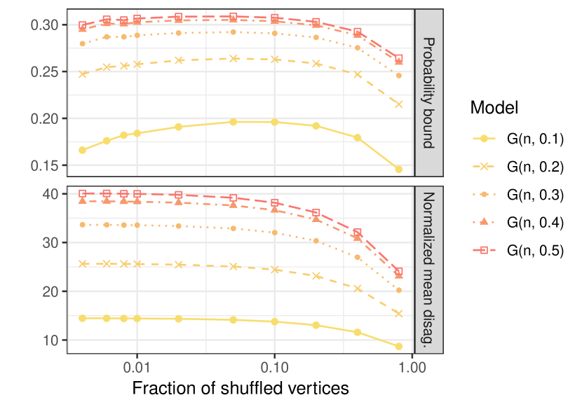
(a) Erdős-Rényi G($n,\alpha$)

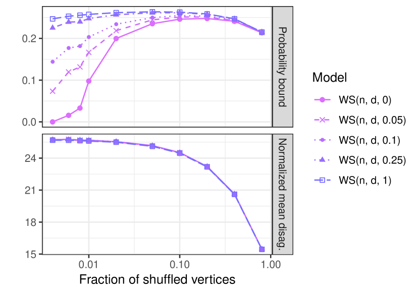
(b) Watts-Strogatz WS($n,d,\beta$)

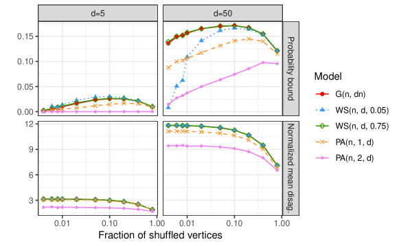
(c) Comparison of different random graph models.

Figure 1: Measures of matching feasibility for different random graph models as a function of the fraction of randomly shuffled vertices $k/n$. The top left figure compares Erdős-Renyi graphs G($n,\alpha$) with different edge probability $\alpha$. The top right figure shows the Watts-Strogatz model WS($n,d,\beta$) with different rewiring probabilities $\beta$. The bottom figure compares these two models and the preferential attachment model with exponent $\gamma$ (PA($\gamma,d$)) for a fixed degree $d$. In each figure, the top panel shows an upper bound on the corrupting probability $p$ tolerated by the graph, and the bottom panel shows the normalized mean edge disagreements after shuffling $k$ random vertices. The plots suggest that graph matching is more feasible in denser and less structured graphs similar to ER.

In the second experiment, we compare the same statistics across different popular random graph models, fixing the expected average degree across the graphs. In particular, we use again the ER model G($n,m$) but now with $m$ fixed edges and the WS model. We additionally include the preferential attachment PA($n,\gamma$,d) model proposed by (Albert and Barabási, 2002). This model creates a graph by a random process in which a new vertex with $d$ edges is added to the graph on each step $t$. For each new vertex the probability that it connects to an existing vertex $i$ is proportional to $d_{it}^{-\gamma}$, where $d_{it}$ is the degree of vertex $i$ at time $t$, and $\gamma\geq 0$ is a constant that controls the preferential effect. Larger values of $\gamma$ increase the preference of new vertices to connect with high degree vertices.

As observed in the previous experiment, the edge density of the graph plays an important role for matching feasibility. Thus, to make fair comparisons between the different models we adjust the model parameters to generate graphs with the same average degree $d$, by fixing $d=5$ (1% density) and $d=50$ (10% density). For the WS model, we generate graphs from a $\text{WS}(n,d,0.05)$ and $\text{WS}(n,d,0.75)$, and for the PA model, we change the exponent $\gamma$ to generate $\text{PA}(n,1,d)$ and $\text{PA}(n,2,d)$. In all cases, we use the default implementation of igraph (Csardi and Nepusz, 2006) to simulate the graphs. The results of these experiments are shown in Figure 1(c). We observe that in general the graphs that have a more random structure (the ER model and the WS model with a large rewiring probability) are the ones in which the measures of matching feasibility are larger. Matching in the PA model is complicated due to the low degree of many vertices, and thus the theoretical probability bound for perfect matchability is low.

5.2 Real-world networks

We also analyze graph matching in the corrupting channel model for real-world networks from different domains. The networks that we use are the Zachary’s karate club friendship network (Zachary, 1977), the graph of synapses between neurons of the C. elegans roundworm (Watts and Strogatz, 1998), the graph of hyperlinks between political blogs from the 2004 US election (Adamic and Adar, 2005), a protein-protein interaction network in yeast (Von Mering et al., 2002), and a citation network between arXiv papers in the condensed matter section (Newman, 2001). Some graph statistics to summarize the data are included in Table 1. These include the number of nodes $n$, the average node degree $d=\frac{1}{n}\sum_{ij}A_{ij}$, the density of the graph $d/(n-1)$, the clustering coefficient $C$ which counts the number of triangles in the graph divided over the maximum number of triangles possible, the skewness $\gamma_{1}$ and the relative standard deviation (RSD) of the degree distribution. In general, as observed in the simulations, we should expect that as the graphs become denser and with a more random structure (lower clustering coefficient and homogeneous degrees), matching becomes more feasible.

Network	$n$	$d$	Density	$C$	$\gamma_{1}$	RSD
Karate	34	4.588	0.14	0.25	2.00	0.84
C. elegans	297	15.79	0.05	0.181	3.50	0.88
Pol. blogs	1,222	27.35	0.02	0.226	3.06	1.4
Prot. interaction	2,617	9.06	0.003	0.47	3.96	1.65
arXiv	16,726	6.69	0.0004	0.36	4.07	0.96

Table 1: Summary statistics of the network data: number of vertices ($n$), average vertex degree ($d$), density of the graph , clustering coefficient ($C$), skewness ($\gamma_{1}$) and relative standard deviation (RSD) of degree distribution .

Figure 2 shows the bounds in the channel probability $\hat{p}_{k}(A)$ (top panel) and the normalized average number of edge disagreements $\hat{X}_{k}(A)$ (bottom panel) for the selected networks. When the fraction of shuffled vertices is small, all networks have a zero tolerance for noise in the corrupting channel model, which can be due to the periphery nodes and the existence of (near) graph automorphisms between some of the vertices. Thus, exactly solving the graph matching problem in general is not feasible if $p>0$. However, as the fraction of shuffled vertices gets larger the value of $\hat{p}_{k}(A)$ increases for some of the networks, which suggests that partial matching is still possible. The political blogs and the C. elegans networks have the highest values for the measured quantities, $\hat{X}_{k}(A)$ and $\hat{p}_{k}(A)$, which can be explained by their large average degree and small clustering coefficient. On the other hand, the protein-protein interaction and arXiv citation networks have the lowest values, possibly because of their low density. The probability bounds in the karate network might be very conservative since the results of Theorem 4 are asymptotic, and $n$ is small for this network.

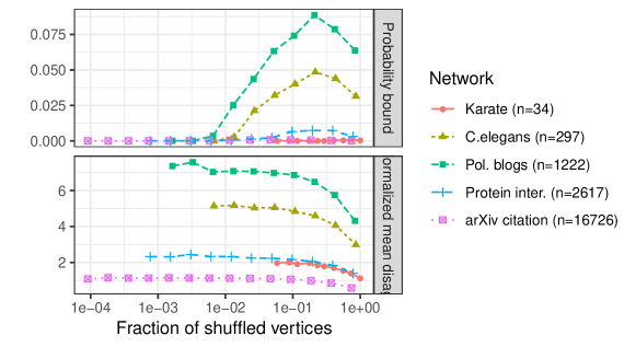
Figure 2: Measures of matching feasibility for different real-world networks as a function of the fraction of shuffled vertices $k/n$. These measures increase with a large number of shuffled vertices, suggesting that partial matching is possible.

In practice, computing the MLE of the unshuffling permutation is computationally unfeasible, as solving the GMP requires to optimize a loss function over $\Pi_{n}$. Thus,

To validate the results above, we measure the accuracy of a graph matching solution of the problem (1) given graphs $A$ and $B$, where $B$ is generated using a uniformly corrupting channel $(p,I)$. Then, we perform graph matching using the FAQ programming algorithm ; we use the true parameter $I$ as the initialization value of the FAQ algorithm in order to check whether $I$ (the unshuffling permutation) is a local minimum of the matching objective function. While this is not finding a globally optimal solution to the graph matching problem in general, this strategy provides a useful surrogate for the difficulty/feasibility of the deanonymization task.

For each network $A$, we generate 30 independent random graphs $B$ from the uniformly corrupting channel with the same value of $p$, and measure the average matching accuracy of the solution $\hat{P}^{\text{FAQ}}$. This process is repeated for different values of $p\in\{10^{-3},10^{-2.5},\ldots,10^{-0.5}\}$. The accuracy of the solution is measured in two ways: First, we calculate the total matching accuracy as the percentage of vertices that are correctly matched; i.e., we compute $\frac{1}{n}\sum_{i=1}^{n}\textbf{1}(\hat{P}^{\text{FAQ}}_{ii}=1)$. As mentioned in Section 4, matching periphery vertices is usually hard in practice, thus, we also investigate whether it is possible to correctly match the core vertices by measuring the accuracy of matching the vertices with the highest degrees. If $j_{1},\ldots,j_{n}$ is an ordering of the vertex indexes according to their degree, so that $\sum_{i=1}^{n}A_{j_{u}i}\geq\sum_{i=1}^{n}A_{j_{v}i}$ if $u<v$, then the accuracy of matching a fraction $c$ of the vertices with the highest degree is given by $\frac{1}{\lfloor cn\rfloor}\sum_{i=1}^{\lfloor cn\rfloor}\textbf{1}(\hat{P}^{\text{FAQ}}_{j_{i}j_{i}}=1)$, with $c\in(0,1]$.

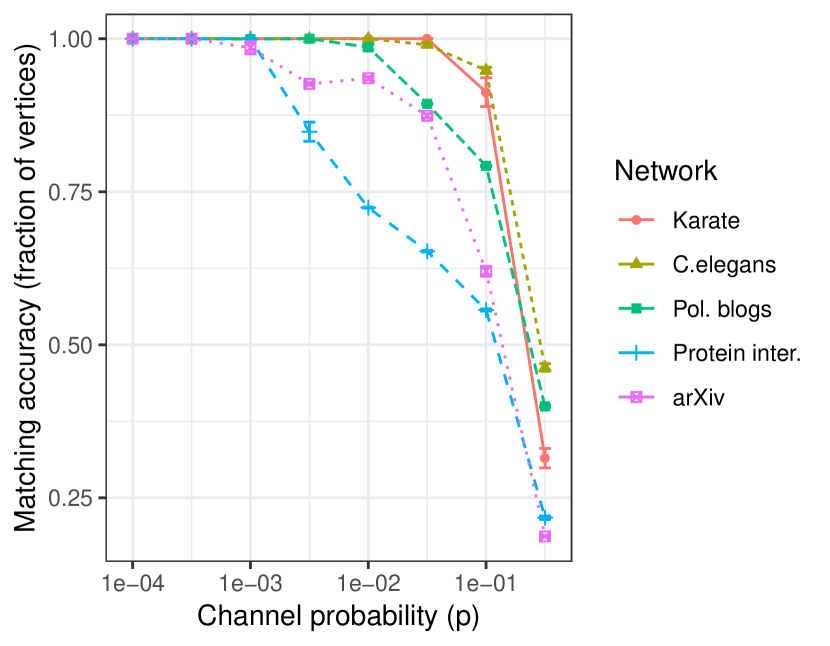
(a) Overall matching accuracy

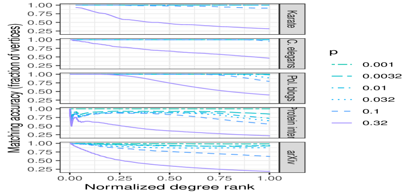
(b) Matching accuracy by degree

Figure 3: Matching accuracy calculated as the fraction of vertices that are correctly matched. The left plot shows the accuracy of matching correctly all the vertices as a function of the channel probability. In the right plot, vertices are ranked from highest to lowest degree, and the accuracy is calculated considering only the vertices with a normalized degree rank smaller than $c\in(0,1]$. The plots show the resulting accuracy as a function of the fraction $c$ of vertices considered, and for different values of the corrupting channel probability $p$.

The overall matching accuracy and the matching accuracy of the vertices with highest degrees are shown in Figures 3(a) and 3(b). When looking to all the vertices aggregated in Figure 3(a), the accuracy in the arXiv and protein interaction networks decreases fast as $p$ increases, which agrees with the predicted matching feasibility of Figure 2. The Karate and C. elegans networks have the highest matching accuracy for most of the values of $p$. This suggests that the bound obtained in Theorem 4 might be conservative for networks with a small number of vertices. However, when looking only to the vertices with the highest degree (Figure 3(b)), the matching accuracy is higher in the political blogs networks, in which almost 25% of the vertices with the highest degree can be matched accurately even for large values of $p$; this is as expected by the results on Figure 2 in which this network is the more resistant to noise for large values of $k$. Figure 3(b) also shows the difficulty of matching vertices in the protein-protein interaction and arXiv citation networks, in which even the vertices with the highest degrees are usually incorrectly matched. This is especially true for the protein-protein interaction network, which has a core-periphery structure in which high-degree nodes are highly connected between each other. As observed in Table 1, this graph is characterized by a large clustering coefficient and a heavy tailed degree distribution.

6 Discussion

The inexact graph matching problem aims to find the alignment that minimizes the number of edge disagreements between a pair of graphs. In this paper, we have shown that this intuitive notion of matching coincides with a maximum likelihood estimator in errorfully observed graphs, which is formally defined using the corrupting channel model. This model is able to accommodate different correlation structures between the edges of a pair of graphs, and many other popular models for the paired and correlated networks are encompassed by this framework. Within this model, we derive necessary and sufficient conditions to determine whether the MLE is consistent, and introduce a relaxed notion of consistency in which all but a small fraction of the vertices are correctly matched.

Since the distribution of the corrupting channel model conditions on a given graph $A$, the consistency results we presented here only depend on the structure of $A$ and the channel noise. This property allowed us to derive conditions that can be used to check whether the MLE is consistent for a given family of graphs, and hence whether it is feasible to solve the GMP. We used these results to study matching feasibility in some popular random graph models, unifying some previous matchability results within our framework and introducing some new ones as well. Our results were tested in simulated and real networks, and we introduced a statistic that can be used in practice to estimate matching feasibility. In addition, we believe that our results can be used to study the feasibility of solving the GMP in other graph models of interest.

This paper studies the information limits of the graph matching problem in the corrupting channel model, and currently there is no known efficient algorithm for finding the solution to the graph matching problem in this model framework. Hence, finding a polynomial-time algorithm to solve the GMP in this model and studying the corresponding computational limits are important open questions for future work. These questions have been partially addressed in a number of settings (see for example Lyzinski et al. (2014b); Shirani et al. (2017); Zhang (2018b, a)), but existing methods usually require seeds to initialize the method, or impose restrictive constraints in the type of graphs or edge correlations that can be handled. Our framework offers a new insight which can be potentially useful in this direction.

Acknowledgements: This material is based on research sponsored by the Air Force Research Laboratory and DARPA, under agreement number FA8750-18-2-0035. The U.S. Government is authorized to reproduce and distribute reprints for Governmental purposes notwithstanding any copyright notation thereon. The views and conclusions contained herein are those of the authors and should not be interpreted as necessarily representing the official policies or endorsements, either expressed or implied, of the Air Force Research Laboratory and DARPA, or the U.S. Government.

Appendix A Proof of main results

A.1 Proof of Theorems 4 and 9

Note that we will prove the more general Theorem 9 here, with the proof of Theorem 4 then following immediately as a special case.

Proof of Theorem 9 part i..

We will first prove part i. of the theorem. We show that under the conditions of the theorem, with high probability we have

$$\|A_{n}-P_{n}^{T}B_{n}P_{n}\|_{F}^{2}\leq\|A_{n}-Q_{n}^{T}P_{n}^{T}B_{n}P_{n}Q_{n}\|_{F}^{2},$$ (19)

for any $Q_{n}\neq I_{n}$, where $I_{n}$ is the identity matrix. The proof proceeds by expressing the difference between the left and the right hand side of Equation (19) can be expressed as a sum of independent random variables, and the tail of its distribution can be sufficiently bounded to show that Equation (19) holds.

Observe that $P_{n}^{T}B_{n}P_{n}\sim C(A_{n},\Psi_{n}^{(1)},\Psi_{n}^{(2)},I_{n})$, so to this end, for a graph $A\in\mathcal{G}_{n}$, define $\widetilde{B}\sim C(A,\Psi_{n}^{(1)},\Psi_{n}^{(2)},I_{n})$ to be the channel corrupted $A$ with parameters $(\Psi_{n}^{(1)},\Psi_{n}^{(2)},I_{n})$. For each $Q\in\Pi_{n}$, define

$$X_{Q}(A) =X_{Q}:=\frac{1}{2}\|A-Q^{T}AQ\|^{2}_{F}$$

$$\widehat{X}_{Q}(A) =\widehat{X}_{Q}:=\frac{1}{2}(\|A-Q^{T}\widetilde{B}Q\|^{2}_{F}-\|A-\widetilde{B}\|^{2}_{F}).$$

Consider a fixed $Q^{T}\in\Pi_{n,k}$, and let the permutation associated with $Q^{T}$ be denoted via $\sigma$. Note that for any matrix $M\in\mathbb{R}^{n\times n}$, $[Q^{T}MQ]_{ij}=M_{\sigma(i),\sigma(j)}$. Recall that $V$ is the set of all vertices, which is isomorphic to $[n]$, and denote by $\binom{V}{2}=\{(i,j)\in[n]\times[n],i<j\}$ to the set of vertex pairs. Letting

$$\Delta_{1} :=\left|\left\{\,\,\{i,j\}\in\binom{V}{2}\text{ s.t. }A_{i,j}\neq A_{\sigma(i),\sigma(j)},\,A_{i,j}=\widetilde{B}_{\sigma(i),\sigma(j)}\right\}\right|$$

$$\Delta_{2} :=\left|\left\{\,\,\{i,j\}\in\binom{V}{2}\text{ s.t. }A_{i,j}=A_{\sigma(i),\sigma(j)},\,A_{i,j}\neq\widetilde{B}_{\sigma(i),\sigma(j)}\right\}\right|,$$

we have that

$$\frac{1}{2}\|A-Q^{T}\widetilde{B}Q\|^{2}_{F} =X_{Q}+\Delta_{2}-\Delta_{1},$$

$$\frac{1}{2}\|A-\widetilde{B}\|^{2}_{F} =\frac{1}{2}\|Q^{T}AQ-Q^{T}\widetilde{B}Q\|^{2}_{F}=\Delta_{2}+\Delta_{1}.$$

And hence $\widehat{X}_{Q}=X_{Q}-2\Delta_{1}$. Let $\tilde{\Delta}_{1}\sim\text{Binom}(X_{Q},\tilde{p}_{n})$ be an independent binomial random variable. Noting that $\Delta_{1}\sim\sum_{i=1}^{X_{Q}}\text{Ber}(q_{i})$ is a sum of independent Bernoulli random variables, with parameters $q_{i}\leq\tilde{p}_{n}$ (each $q_{i}$ is equal to its corresponding corrupting probability $\Psi^{(k)}_{i^{\prime}j^{\prime}}$, which is upper bounded by $\tilde{p}$), we have that $\mathbb{P}(\Delta_{1}\geq\tau)\leq\mathbb{P}(\tilde{\Delta}_{1}\geq\tau)$ for all $\tau\geq 0$, and hence

$$\mathbb{P}(\widehat{X}_{Q}\leq 0) =\mathbb{P}(\Delta_{1}\geq X_{Q}/2)\leq\text{exp}\left\{-X_{Q}H(1/2,\tilde{p}_{n})\right\}$$

$$=\text{exp}\left\{\frac{1}{2}X_{Q}\log(4\tilde{p}_{n}(1-\tilde{p}_{n}))\right\},$$ (20)

where $H(1/2,p)$ is the relative binomial entropy (Arratia and Gordon, 1989, Theorem 1). If $n\geq n_{1}$, then the Assumption in Eq. 5 implies

$$\mathbb{P}(\widehat{X}_{Q}\leq 0)\leq\text{exp}\left\{-3k\log(n)\right\},$$ (21)

and this bound holds uniformly for all $Q^{T}\in\Pi_{n,k}$.

Consider now $n\geq n_{1}$. Let $B_{n}\sim C(A_{n},\Psi^{(1)}_{n},\Psi^{(2)}_{n},P_{n})$ and $\widetilde{B}_{n}\sim C(A_{n},\Psi^{(1)}_{n},\Psi^{(2)}_{n},I_{n})$. For each $Q\in\Pi_{n}$, let

$$\widehat{Y}_{Q}(A) =\widehat{Y}_{Q}:=\frac{1}{2}(\|A_{n}-Q^{T}B_{n}Q\|^{2}_{F}-\|A_{n}-P_{n}^{T}B_{n}P_{n}\|^{2}_{F})$$

$$\widehat{X}_{Q}(A) =\widehat{X}_{Q}:=\frac{1}{2}(\|A_{n}-Q^{T}\widetilde{B}_{n}Q\|^{2}_{F}-\|A_{n}-\widetilde{B}_{n}\|^{2}_{F}).$$

Note that $\widehat{X}_{P_{n}^{T}Q}=\widehat{Y}_{Q}$, and hence,

$$\mathbb{P}(\exists\,Q\neq P_{n}\text{ s.t. }\widehat{Y}_{Q}\leq 0) =\mathbb{P}(\exists\,P_{n}^{T}Q\neq I\text{ s.t. }\widehat{X}_{P_{n}^{T}Q}\leq 0)$$

$$=\mathbb{P}(\exists\,\tilde{Q}\neq I\text{ s.t. }\widehat{X}_{\tilde{Q}}\leq 0)$$

For each $k>1$, note that $|\Pi_{n,k}|\leq n^{k}$. For each $k$, applying Eq. (21) uniformly for each $\tilde{Q}\in\Pi_{n,k}$ and summing over $k$ yields

$$\mathbb{P}(\exists\,\tilde{Q}\neq I\text{ s.t. }\widehat{X}_{\tilde{Q}}\leq 0)\leq\sum_{k=2}^{n}\text{exp}\left\{-2k\log n\right\}\leq\text{exp}\left\{-4\log n+\log n\right\}=n^{-3},$$ (22)

and therefore

$$\mathbb{P}(\exists\,Q\neq P_{n}\text{ s.t. }\widehat{Y}_{Q}\leq 0) =\mathbb{P}\left(\operatorname*{arg\,min}_{P\in\Pi_{n}}\|A_{n}-P^{T}B_{n}P\|_{F}^{2}\neq\{P_{n}\}\right)$$ (23)

$$=\mathbb{P}(\exists\,\text{ an MLE, }\widehat{{P}}_{n},\text{ of }P_{n}\text{ s.t. }\widehat{{P}}_{n}\neq P_{n})\leq n^{-3}.$$

Therefore, with probability $1$ it holds that for all but finitely many $n$ (by the Borel-Cantelli lemma as $n^{-3}$ is finitely summable) the unique MLE of $P_{n}$ is $\widehat{{P}}_{n}=P_{n}$, and any sequence of MLE’s, $(\widehat{{P}}_{n})_{n=n_{0}}^{\infty}$, is strongly consistent.

Proof of Theorem 9 part ii. Note that condition Eq. 6 implies

$$\max_{Q_{n}\in S_{n}}\log\left(\frac{1}{4\breve{p}_{n}(1-\breve{p}_{n})}\right)\left(\|A_{n}-Q_{n}^{T}A_{n}Q_{n}\|^{2}_{F}\right)=o\left(\log(n)\right)$$ (24)

As in the proof of part i., we will work with $P_{n}=I_{n}$, as the consistency results for the MLE estimating $I_{n}$ transfer immediately to consistency results for the MLE estimating a more general $P_{n}$ Consider the notation as in the proof of part i, and consider the $\Theta(n)$ disjoint $Q_{n}$ permutations with ${Q_{n}}\in\cup_{i=2}^{k_{n}}\Pi_{n,i}\setminus{I_{n}}$ (where $S_{n}$ be the set of these $Q_{n}$) satisfying Eq. (6), (7) as posited in Theorem 9. Let $Z_{n}=\sum_{Q_{n}\in S_{n,k}}\mathds{1}\{\widehat{X}_{Q}\leq 0\}$.

Let $Q\in S_{n}$ be any of the permutations as defined above. We have that $\Delta_{1}\sim\sum_{i=1}^{X_{Q}}\text{Ber}(q_{i})$ for some independent Bernoulli random variables with parameters $\breve{p}_{n}\leq q_{i}\leq\tilde{p}_{n}$, and let $\breve{\Delta}_{1}\sim\text{Binom}(X_{Q},\breve{p}_{n})$. We will make use of the following Theorem from Zhang and Zhou (2018) in our proof.

Theorem 16 (Theorem 9 from Zhang and Zhou (2018)).

Suppose that $X$ is centralized binomial distributed with parameters $(k,p)$. For any $\beta>1$, there exist constants $c_{\beta}$, $C_{\beta}>0$ that only rely on $\beta$, such that

$$\mathbb{P}(X\geq x)\begin{cases}\geq c_{\beta}\text{exp}(-C_{\beta}kh_{p}(p+\frac{x}{k})),&\text{ if }0\leq x\leq\frac{k(1-p)}{\beta}\text{ and }x+kp\geq 1;\\ =1-(1-p)^{k},&\text{ if }0\leq kp+x<1\end{cases}$$ (25)

$$\mathbb{P}(X\leq-x)\begin{cases}\geq c_{\beta}\text{exp}(-C_{\beta}kh_{p}(p-\frac{x}{k})),&\text{ if }0\leq x\leq\frac{kp}{\beta}\text{ and }x+k(1-p)\geq 1;\\ =1-p^{k},&\text{ if }0\leq k(1-p)+x<1\end{cases}$$ (26)

where $h_{u}(v)=v\log(v/u)+(1-v)\log(\frac{1-v}{1-u})$.

In the notation of the above theorem, let $X=\breve{\Delta}_{1}-X_{Q}\breve{p}_{n}$ (so that $k=X_{Q}$ and $p=\breve{p}_{n}$) and $x=X_{Q}(1/2-p_{n})$. We have that

$$x=X_{Q}(1/2-\breve{p}_{n})\leq X_{Q}(1-\breve{p}_{n})/2,$$

and we can take $\beta=2$. Applying Eq. (25) and the fact that $\mathbb{P}(\breve{\Delta}_{1}\geq\tau)\leq\mathbb{P}(\Delta_{1}\geq\tau)$ for all $\tau\geq 0$, then implies (where $c$ and $C$ are constants independent of $n$)

$$p_{Q}:=\mathbb{P}(\Delta_{1}\geq X_{Q}/2) \geq\mathbb{P}(\breve{\Delta}_{1}-X_{Q}\breve{p}_{n}\geq X_{Q}(1/2-\breve{p}_{n}))$$

$$\geq c\text{ exp}\left\{-CX_{Q}\frac{1}{2}\log\left(\frac{1}{4\breve{p}_{n}(1-\breve{p}_{n})}\right)\right\}$$

$$=\Omega\left(c\text{ exp}\left(-\frac{1}{2}\log(n)\right)\right)$$ (27)

where the last line follows from Eq. (24).

Consider now disjoint $Q=Q_{n}$ and $Q^{\prime}=Q_{n}^{\prime}$ in $S_{n,k_{n}}$. Each $\widehat{X}_{Q}=\sum_{i,j}A_{i,j}(B_{i,j}-B_{\sigma_{Q}(i),\sigma_{Q}(j)})$ is a function of $\Theta(nk_{n})$ independent Bernoulli random variables (the $B_{i,j}$ that are permuted). The disjointedness of $Q$ and $Q^{\prime}$ implies that there are at most $2k^{2}$ common $B_{i,j}$ that appear in both $\widehat{X}_{Q}$ and $\widehat{X}_{Q^{\prime}}$, and we can decompose $\widehat{X}_{Q^{\prime}}$ into

$$\widehat{X}_{Q^{\prime}}=Y+W,$$

where $Y$ is independent of $\widehat{X}_{Q}$ and $|W|\leq 2k_{n}^{2}$. Note that $k_{n}=\Theta(1)$ by construction. We then have that (where $\Delta_{1}^{\prime}$ is the $\Delta_{1}$ associated with $\widehat{X}_{Q^{\prime}}$)

$$\operatorname{Cov}\left(\mathds{1}\{\widehat{X}_{Q}\leq 0\},\mathds{1}\{\widehat{X}_{Q^{\prime}}\leq 0\}\right) =\mathbb{P}(\widehat{X}_{Q}\leq 0,\widehat{X}_{Q^{\prime}}\leq 0)-\mathbb{P}(\widehat{X}_{Q}\leq 0)\mathbb{P}(\widehat{X}_{Q^{\prime}}\leq 0)$$

$$\leq\mathbb{P}(Y\leq 2k_{n}^{2},\widehat{X}_{Q^{\prime}}\leq 0)-\mathbb{P}(Y\leq-2k^{2})\mathbb{P}(\widehat{X}_{Q}\leq 0)$$

$$=\mathbb{P}(\widehat{X}_{Q}\leq 0)\mathbb{P}(-2k_{n}^{2}\leq Y\leq 2k_{n}^{2})$$

$$\leq\mathbb{P}(\widehat{X}_{Q}\leq 0)\mathbb{P}(-4k_{n}^{2}\leq\widehat{X}_{Q^{\prime}}\leq 4k_{n}^{2})$$

$$=p_{Q}\mathbb{P}(X_{Q^{\prime}}/2-2k_{n}^{2}\leq\Delta_{1}^{\prime}\leq X_{Q^{\prime}}/2+2k_{n}^{2})$$ (28)

Observe that conditions (13) and (14) imply that that $X_{Q}=\omega(1)$ and that $(1/2-\breve{p}_{n})^{2}=o(1)$. The variable $\Delta_{1}^{\prime}=\sum_{i=1}^{X_{Q^{\prime}}}\text{Ber}(q_{i})$ is a sum of $X_{Q^{\prime}}$ independent binary variables with $\breve{p}_{n}\leq q_{i}\leq\tilde{p}_{n}$, and therefore, by the Lindeberg-Feller’s Central Limit Theorem, $s_{n}^{-1}(\Delta_{1}^{\prime}-\mathbb{E}[\Delta_{1}^{\prime}])$ converges in distribution to a standard normal, with

$$X_{Q^{\prime}}\breve{p}_{n}\leq\mathbb{E}[\Delta_{1}^{\prime}]\leq X_{Q^{\prime}}\tilde{p}_{n},$$

$$X_{Q^{\prime}}\breve{p}_{n}(1-\breve{p}_{n})\leq s_{n}^{2}\leq X_{Q^{\prime}}\tilde{p}_{n}(1-\tilde{p}_{n}).$$

Therefore, setting $H_{n}:=\sqrt{X_{Q^{\prime}}}\left(\frac{1/2-\mathbb{E}[\Delta_{1}^{\prime}]/X_{Q^{\prime}}}{s_{n}/\sqrt{X_{Q^{\prime}}}}\right)$, we have that for $n$ sufficiently large

$$\mathbb{P}\left(\Delta_{1}^{\prime}-\frac{X_{Q^{\prime}}}{2}\in\left[-2k_{n}^{2},2k_{n}^{2}\right]\right) =\mathbb{P}\left(\frac{\Delta_{1}^{\prime}-\mathbb{E}[\Delta_{1}^{\prime}]}{s_{n}}\in\left[H_{n}-\frac{2k_{n}^{2}}{s_{n}},H_{n}+\frac{2k_{n}^{2}}{s_{n}}\right]\right)$$

$$\leq C_{1}\frac{k_{n}^{2}}{s_{n}}\leq\frac{C_{2}}{\sqrt{X_{Q^{\prime}}}}.$$

for some constants $C_{1},C_{2}$. Combining this bound with Equation (28), we have

$$\operatorname{Cov}\left(\mathds{1}\{\widehat{X}_{Q}\leq 0\},\mathds{1}\{\widehat{X}_{Q^{\prime}}\leq 0\}\right)\leq C_{2}p_{Q}\frac{1}{\sqrt{X_{Q^{\prime}}}}$$

We now have that

$$\text{Var}(Z_{n})\leq\mathbb{E}(Z_{n})+\sum_{Q_{n}\in S_{n,k}}\sum_{Q^{\prime}_{n}\neq Q_{n}}p_{Q_{n}}\frac{C}{\sqrt{X_{Q_{n}^{\prime}}}}.$$

The second moment method (see Alon et al. (1997) Theorem 4.3.1) can be applied to show

$$\mathbb{P}(\exists\,Q_{n}\in\Pi_{n,k_{n}}\text{ s.t. }\widehat{X}_{Q_{n}}\leq 0) =\mathbb{P}(Z_{n}>0)\geq 1-\frac{\text{Var}(Z_{n})}{(\mathbb{E}Z_{n})^{2}}$$

$$\geq 1-\frac{\mathbb{E}Z_{n}}{(\mathbb{E}Z_{n})^{2}}-\frac{\sum_{Q_{n}\in S_{n,k}}\sum_{Q^{\prime}_{n}\neq Q_{n}}p_{Q_{n}}\frac{C}{\sqrt{X_{Q_{n}^{\prime}}}}}{\sum_{Q_{n}}\sum_{Q^{\prime}_{n}}p_{Q_{n}}p_{Q_{n}^{\prime}}}.$$

By the assumption in Eq. (27), we have that

$$\mathbb{E}(Z_{n})=\Omega(ne^{-\frac{1}{2}\log n})=\omega(1),$$

By the assumption in Eq.(14), we have that $\breve{p}_{n}\rightarrow\frac{1}{2}$ (otherwise, the left hand side of Eq. (14) is at least of a constant order). Combining this fact with $\breve{p}_{n}\leq\tilde{p}_{n}$ and Eq. (13), we have that $\min_{Q_{n}\in S_{n}}\|A_{n}-Q_{n}^{T}A_{n}Q_{n}\|_{F}^{2}=\omega(1)$. Combining these facts, we have that for each $Q\in S_{n}$,

$$-X_{Q}\log\left(\frac{1}{4\breve{p}_{n}(1-\breve{p}_{n})}\right)+\log(X_{Q}) =\log(X_{Q})\left(1-\frac{X_{Q}}{\log X_{Q}}\log\left(\frac{1}{4\breve{p}_{n}(1-\breve{p}_{n})}\right)\right)$$

$$\geq\log(X_{Q})\left(1-\max_{Q\in S_{n}}\frac{X_{Q}}{\log X_{Q}}\log\left(\frac{1}{4\breve{p}_{n}(1-\breve{p}_{n})}\right)\right)$$

$$\geq\min_{Q\in S_{n}}\log(X_{Q})\left(1-o(1)\right)$$

$$=\omega(1).$$

Let

$$m_{n}:=\min_{Q\in S_{n}}-X_{Q}\log\left(\frac{1}{4\breve{p}_{n}(1-\breve{p}_{n})}\right)+\log(X_{Q}),$$

and note that $m_{n}=\omega(1)$. Therefore,

$$\frac{1/\sqrt{X_{Q^{\prime}}}}{p_{Q^{\prime}}} \leq c\frac{1}{\sqrt{X_{Q^{\prime}}}}\text{ exp}\left\{CX_{Q^{\prime}}\frac{1}{2}\log\left(\frac{1}{4\breve{p}_{n}(1-\breve{p}_{n})}\right)\right\}$$

$$=c\,\text{exp}\left\{CX_{Q^{\prime}}\frac{1}{2}\log\left(\frac{1}{4\breve{p}_{n}(1-\breve{p}_{n})}\right)-\frac{1}{2}\log(X_{Q^{\prime}})\right\}$$

$$\leq c\,\text{exp}\{-Cm_{n}\}=o(1).$$

We then have that

$$\frac{\sum_{Q_{n}\in S_{n,k}}\sum_{Q^{\prime}_{n}\neq Q_{n}}p_{Q_{n}}\frac{1}{\sqrt{X_{Q_{n}^{\prime}}}}}{\sum_{Q_{n}}\sum_{Q^{\prime}_{n}}p_{Q_{n}}p_{Q_{n}^{\prime}}} \leq c\,\text{exp}\{-Cm_{n}\}\frac{\sum_{Q_{n}\in S_{n,k}}\sum_{Q^{\prime}_{n}\neq Q_{n}}p_{Q_{n}}p_{Q_{n}^{\prime}}}{\sum_{Q_{n}}\sum_{Q^{\prime}_{n}}p_{Q_{n}}p_{Q_{n}^{\prime}}} =o(1).$$

$$\mathbb{P}(\exists\,Q_{n}\in S_{n}\text{ s.t. }\widehat{X}_{Q_{n}}\leq 0)=\mathbb{P}(Z_{n}>0)\geq 1-o(1).$$

Therefore, for any $1>\epsilon>0$

$$\mathbb{P}(\max_{P\in\mathcal{P}^{*}}\|P-I_{n}\|_{F}^{2}\leq\epsilon)\rightarrow 0$$

giving the desired inconsistency result.

Proof of Theorem 9 part iii. As in the proofs of part i. and ii., we will work with $P_{n}=I_{n}$, as the consistency results for the MLE estimating $I_{n}$ transfer immediately to consistency results for the MLE estimating a more general $P_{n}$. Consider the notation as in the proof of parts i. and ii. To prove part iii., consider first the case that $\breve{p}_{n}$ is bounded away from zero. Note that in this case, Equation (15) (combined with the bound in Eq. (25), and the fact that $\breve{\Delta}_{1}$ is stochastically less or equal than $\Delta_{1}$) implies that

$$p_{Q_{n}}\begin{cases}\geq c\text{ exp}\left\{-CX_{Q_{n}}\frac{1}{2}\log\left(\frac{1}{4\breve{p}_{n}(1-\breve{p}_{n})}\right)\right\}=\Theta(1)&\text{ if }X_{Q_{n}}/2\geq 1\\ \geq 1-(1-\breve{p}_{n})^{X_{Q_{n}}}=\Theta(1)&\text{ if }X_{Q_{n}}/2<1\\ \end{cases}$$

On the other hand, if $\breve{p}_{n}\rightarrow 0$ as $n$ goes to infinity, then Equation (15) implies that $X_{Q_{n}}=o(1)$, and hence there exists infinitely many $n$’s for which $X_{Q_{n}}=0$ and the MLE would not be uniquely defined. Therefore, for any $1>\epsilon>0$

$$\limsup\mathbb{P}(\max_{P\in\mathcal{P}^{*}}\|P-I_{n}\|_{F}^{2}\leq\epsilon)<1$$

and so the MLE is not weakly consistent. ∎

Proof of Theorem 4.

Observe that under the settings of the theorem, using the notation of Theorem 9 we have that

$$\tilde{p}_{n}=p_{n}=\breve{p}_{n}.$$

From this observation, the result follows. ∎

A.2 Proof of Corollary 6

Proof.

By Lemma 4 in Lyzinski et al. (2016a), we have that for $n$ sufficiently large and all $Q\in\Pi_{n,k}$,

$$\mathbb{P}\left(\|A_{n}-Q^{T}A_{n}Q\|_{F}^{2}\leq\frac{\alpha_{n}kn}{3}\right)\leq 2\exp\left(-\alpha_{n}^{2}kn/128\right).$$ (29)

Note that for sufficiently large $n$, the condition of the corollary implies that

$$\frac{6k\log n}{-\log(4p_{n}(1-p_{n}))}\leq\frac{6k\log n}{(1/2-p_{n})^{2}}\leq\frac{\alpha_{n}kn}{3}.$$

The same condition also implies that $\alpha_{n}=\omega\left(\sqrt{\log n/n}\right)$, and combining these facts with Equation (29), we have that

$$\mathbb{P}\left(\min_{Q\in\Pi_{n,k}}\|A_{n}-Q^{T}A_{n}Q\|_{F}^{2}\leq\frac{-6k\log n}{\log(4p_{n}(1-p_{n}))}\ \forall k\in[n]\right) \leq\sum_{k=2}^{n}\sum_{Q\in\Pi_{n,k}}\exp\left(-\frac{\alpha_{n}^{2}kn}{128}\right)$$

$$\leq\sum_{k=2}^{n}\exp\left(k\log n-4k\log n\right)$$

$$\leq\frac{1}{n^{2}}$$

for $n$ sufficiently large. As in the proof of Theorem 4 part i., the result follows from an application of the Borell-Cantelli lemma. ∎

A.3 Proof of Corollary 8

Proof.

To prove part a), define $P^{(i)}$ as the permutation that only switches vertices $i$ and $i+1$, i.e., $P^{(i)}_{i,i+1}=P^{(i)}_{i+1,i}=1$ and $P^{(i)}_{jj}=1$ for $j=\in[n]\setminus\{i,i+1\}$, and let

$$S_{n}=\{P^{(i)}:i\ \text{mod }2=1\}=\begin{cases}\{P^{(1)},P^{(3)},\cdots,P^{(n-1)}\}\text{ if }n\text{ is even}\\ \{P^{(1)},P^{(3)},\cdots,P^{(n-2)}\}\text{ if }n\text{ is odd}\end{cases}$$

be a set of disjoint permutations of this type. Without loss of generality, take $P=P^{(1)}$. Then

$$\frac{1}{4}\|A-P^{T}AP\|_{F}^{2} =\sum_{j=3}^{n}\left(A_{j2}-A_{j1}\right)^{2}$$

$$=(1-A_{d_{n}+2,1})^{2}+(A_{n-d_{n}+1,2}-1)^{2}+\sum_{j=d_{n}+3}^{n-d_{n}}\left(A_{j2}-A_{j1}\right)^{2},$$

which is a sum of $n-2d_{n}$ independent Bernoulli random variables; namely

$$(1-A_{d_{n}+2,1})^{2} \sim\text{Bern}(1-\beta_{n});$$

$$(A_{n-d_{n}+1,2}-1)^{2} \sim\text{Bern}(1-\beta_{n});$$

$$\left(A_{j2}-A_{j1}\right)^{2} \sim\text{Bern}(2\beta_{n}(1-\beta_{n}))\text{ for }d_{n}+3\leq j\leq n-d_{n}.$$

If $n-2d_{n}=O(1)$, then part iii. of Theorem 4 completes the proof. Hence, consider $n-2d_{n}=\omega(1)$. Define

$$f(\beta_{n}) :=\frac{1}{4}\mathbb{E}\|AP-PA\|^{2}_{F}+\sqrt{2n\log n}$$

$$=2(1-\beta_{n})\left[1+(n-2d_{n}-2)\beta_{n}\right]+\sqrt{2n\log n}$$

$$=o\left(\frac{\log n}{(1/2-p_{n})^{2}}\right),$$

where the last equality follows from the assumptions on the growth rate of $\beta_{n}$ and $p_{n}$. By Hoeffding’s inequality,

$$\mathbb{P}\left(\frac{1}{4}\|A-P^{T}AP\|^{2}_{F}\geq f(\beta_{n})\right)\leq\exp\left(-4\log n\right).$$

Hence,

$$\mathbb{P}\left(\max_{P\in{S}_{n}}\frac{1}{4}\|A-P^{T}AP\|^{2}_{F}\geq f(\beta_{n})\right) \leq \sum_{P\in{S}_{n}}\mathbb{P}\left(\frac{1}{4}\|A-P^{T}AP\|^{2}_{F}\geq f(\beta_{n})\right)$$

$$\leq \frac{n}{2}\exp\left(-4\log n\right)=\frac{1}{2n^{3}}.$$

By the Borell-Cantelli lemma, for all but finitely many $n$, $\max_{P\in\mathcal{S}}\frac{1}{4}\|AP-PA\|^{2}_{F}<f(\beta_{n})=o\left(\frac{\log n}{(1/2-p_{n})^{2}}\right)$, and using Theorem 4 part ii. (resp., part iii.) if $\min_{P\in\mathcal{S_{n}}}\frac{1}{4}\|AP-PA\|^{2}_{F}(1/2-p_{n})^{2}=\omega(1)$ (resp., $\min_{P\in\mathcal{S_{n}}}\frac{1}{4}\|AP-PA\|^{2}_{F}(1/2-p_{n})^{2}=O(1))$, the result follows.

For part b), define a $n\times n$ graph $B$ such that $B_{ij}=A_{ij}$ whenever $|i-j|\text{mod}(n-1-d_{n})\geq d_{n}$, and $B_{ij}=B_{ji}\sim\text{Bern}(\beta_{n})$ otherwise. Then $B\sim\text{G}(n,\beta_{n})$. Consider a permutation $Q\in\Pi_{n,k}$, and observe that

$$2\|A-Q^{T}AQ\|_{F}^{2} =2\|B-Q^{T}BQ+(A-B)-Q^{T}(A-B)Q\|^{2}_{F}$$

$$\geq\|B-Q^{T}BQ\|_{F}^{2}-8kd_{n}=\|B-Q^{T}BQ\|_{F}^{2}-o\left(k\frac{\log n}{(1/2-p_{n})^{2}}\right).$$ (30)

where

$$2\|(A-B)-Q^{T}(A-B)Q\|_{F}^{2}\leq 8kd_{n}$$

follows from $(A-B)$ and $Q^{T}(A-B)Q$ only disagreeing on edges incident to the $k_{n}$ vertices that are permuted by $Q_{n}$, and there are at most $2d_{n}$ such edges per permuted vertex (each being double counted). Since $B$ is an ER graph, following the proof of Corollary 6 mutatis mutatandis, it can be shown that, with probability 1, for all but finitely many $n$

$$\min_{Q\in\Pi_{n,k}}\|B-Q^{T}BQ\|_{F}^{2}\geq\frac{-12k\log n}{\log(4p_{n}(1-p_{n})},$$

and thus

$$\min_{Q\in\Pi_{n,k}}\|A-Q^{T}AQ\|_{F}^{2}\geq\frac{-6k\log n}{\log(4p_{n}(1-p_{n})}+o\left(k\frac{\log n}{(1/2-p_{n})^{2}}\right).$$

The result now follows from Theorem 4 part i. ∎

A.4 Proof of Corollary 10

Proof of Corollary 10.

Let $A\sim\text{G}(n,q_{n})$ be an Erdős-Rényi graph. Given a permutation $Q\in\Pi_{n,k}$ that shuffles exactly $k$ vertices, the number of edge disagreements can be expressed as

$$\frac{1}{2}\|A-Q^{T}AQ\|_{F}^{2} =\sum_{(i,j)\in\mathcal{U}_{Q}}(A_{i,j}-A_{\sigma_{Q}(i),\sigma_{Q}(j)})^{2},$$

where

$$\mathcal{U}_{Q}:=\left\{(i,j)\in\binom{V}{2}:(\sigma_{Q}(i),\sigma_{Q}(j))\neq(i,j)\text{ and }(\sigma_{Q}(i),\sigma_{Q}(j))\neq(j,i)\right\}.$$

To calculate the number of elements in $\mathcal{U}_{Q}$, define the sets

$$\mathcal{U}_{Q}^{(1)} :=\left\{(i,j)\in\binom{V}{2}:\sigma_{Q}(i)\neq i\text{ and }\sigma_{Q}(j)\neq j\right\},$$

$$\mathcal{U}_{Q}^{(2)} :=\left\{(i,j)\in\binom{V}{2}:\sigma_{Q}(i)\neq i\text{ and }\sigma_{Q}(j)=j\right\},$$

$$\mathcal{U}_{Q}^{(3)} :=\left\{(i,j)\in\binom{V}{2}:\sigma_{Q}(i)=j\text{ and }\sigma_{Q}(j)=i\right\},$$

and observe that $\mathcal{U}_{Q}=(\mathcal{U}^{(1)}_{Q}\cup\mathcal{U}^{(2)}_{Q})\setminus\mathcal{U}^{(3)}_{Q}$, where $|\mathcal{U}^{(1)}_{Q}|=\binom{k}{2}$, $|\mathcal{U}^{(2)}_{Q}|=k(n-k)$, and $|\mathcal{U}^{(3)}_{Q}|\leq\frac{k}{2}$. Hence,

$$|\mathcal{U}_{Q}|\geq\frac{k(k-2)}{2}+k(n-k)\geq\frac{nk}{3}.$$

We make use of the following result of Alon et al. (1997) as stated in Lyzinski et al. (2014a).

Theorem 17 (Theorem 3 of Lyzinski et al. (2014a)).

Suppose $X$ is a function of $\eta$ independent Bernoulli$(q)$ random variables such that changing the value of any one of the Bernoulli random variables changes the value of $X$ by at most 2. For any $t:0\ 0\leq t<\sqrt{\eta q(1-q)}$, we have

$$\mathbb{P}\left(|X-\mathbb{E}[X]|>4t\sqrt{\eta q(1-q)}\right)\leq 2\exp(-t^{2}).$$

Using the notation of the theorem above, let $X=\frac{1}{2}\|A-Q^{T}AQ\|_{F}^{2}$, $\eta=|\mathcal{U}_{Q}|$, and observe that

$$\mathbb{E}[X]=\eta\mathbb{P}(A_{ij}\neq A_{\sigma_{Q}(i),\sigma_{Q}(j)})=2\eta q_{n}(1-q_{n})\geq\frac{2nkq_{n}(1-q_{n})}{3}.$$ (31)

By the conditions in the corollary, there exists $n_{0}$ such that for all $n>n_{0}$

$$\frac{nk}{3}q_{n}(1-q_{n})>\frac{6k\log n}{\log\left(\frac{1}{4\tilde{p}_{n}(1-\tilde{p}_{n})}\right)}.$$ (32)

Observe that the assumptions of Theorem 17 hold for any $0\leq t<\sqrt{\eta q_{n}(1-q_{n})}$, and in particular let $t=\frac{1}{4}\sqrt{\frac{nkq_{n}(1-q_{n})}{3}}$. Then, using Theorem 17 in combination with Equations (31) and (32),

$$\mathbb{P}\left(X\leq\frac{6k\log n}{\log\left(\frac{1}{4\tilde{p}_{n}(1-\tilde{p}_{n})}\right)}\right) \leq\mathbb{P}\left(|X-\mathbb{E}[X]|\geq\mathbb{E}[X]-\frac{6k\log n}{\log\left(\frac{1}{4\tilde{p}_{n}(1-\tilde{p}_{n})}\right)}\right)$$

$$\leq\mathbb{P}\left(|X-\mathbb{E}[X]|\geq\frac{1}{3}nkq_{n}(1-q_{n})\right)$$

$$\leq 2\exp\left(-\frac{nkq_{n}(1-q_{n})}{48}\right)$$

By the assumptions in Corollary 10, there exists $n_{1}$ sufficiently large such that for all $n\geq n_{1}$, it holds that $q_{n}(1-q_{n})>\frac{192\log n}{n}$. Therefore, for all $n>\max\{n_{0},n_{1}\}$,

$$\mathbb{P}\left(\min_{Q_{n}\in\Pi_{n,k}}\|A-Q^{T}AQ\|_{F}^{2}\leq\frac{-6k\log n}{\log(4\tilde{p}_{n}(1-\tilde{p}_{n}))}\ \forall k\geq 2\right) \leq\sum_{k=2}^{n}\sum_{Q\in\Pi_{n,k}}2\exp\left(\frac{-nkq_{n}(1-q_{n})}{48}\right)$$

$$\leq\sum_{k=2}^{n}2\exp\left(k\log n-4k\log n\right)$$

$$\leq\frac{2}{n^{2}}.$$

As in the proof of Theorem 9 part i., the result follows from an application of the Borell-Cantelli lemma.

∎

A.5 Proof of Theorem 14

Proof.

The proof of this result follows the proof of Theorem 4 mutatis mutandis by only considering permutations of enough vertices. In particular, the conditions of part i. imply that an analogous to Equations (22) and (23) hold, that is,

$$\mathbb{P}\left(\operatorname*{arg\,min}_{P\in\Pi_{n}}\|A_{n}-P^{T}B_{n}P\|_{F}^{2}\notin\bigcup_{k=k_{n}}^{n}\Pi_{n,k}\right) =\mathbb{P}(\exists\,Q\in\bigcup_{k=k_{n}}^{n}\Pi_{n,k}\text{ s.t. }\widehat{Y}_{Q}\leq 0)$$

$$\leq\sum_{k=k_{n}}^{n}\exp(-2k\log n)$$

$$\leq n^{-3}.$$

Therefore, with probability $1$ it holds that for all but finitely many $n$ (by the Borel-Cantelli lemma as $n^{-3}$ is finitely summable) the MLE of $P_{n}$ is in $\Pi_{n}\setminus\bigcup_{k=k_{n}}^{n}\Pi_{n,k}$, so $\max\|\widehat{{P}}_{n}-P_{n}\|_{F}^{2}\leq k_{n}$, and because $\alpha_{n}=\omega(k_{n})$, the strong $\alpha_{n}$-consistency follows.

∎

A.6 Proof of Corollary 15

Proof.

Let $H\sim$G$(n,d/n)$ be an ER graph with rate $d/n$. Define the events

$$\mathcal{A}_{n,d} =\{\text{ Eq. }\ref{eq:growthrate-quasi}\text{ holds for }A\text{ for all }k=\omega(n^{2/3})\}$$

$$\mathcal{A}_{n,d/n} =\{\text{ Eq. }\ref{eq:growthrate-quasi}\text{ holds for }H\text{ for all }k=\omega(n^{2/3})\}$$

$$\mathcal{R}_{n,d/n} =\{H\text{ is }d\text{-regular}\}$$

We then have that

$$\mathbb{P}(\mathcal{A}_{n,d/n}^{c}) \geq\mathbb{P}(\mathcal{A}_{n,d/n}^{c}|\mathcal{R}_{n,d/n})\mathbb{P}(\mathcal{R}_{n,d/n})=\mathbb{P}(\mathcal{A}_{n,d}^{c})\mathbb{P}(\mathcal{R}_{n,d/n}).$$

Note that for $H_{n}$ in $\Pi_{n,k_{n}}$ with $k_{n}=k=\omega(n^{2/3})$,

• $\|H_{n}-Q^{T}H_{n}Q\|^{2}_{F}$ is a function of $\binom{k}{2}+(n-k)k-O(k)$ independent Bern($p=d/n$) random variables;

• Changing any one of these Bern($p=d/n$) random variables can change $\|H_{n}-Q^{T}H_{n}Q\|^{2}_{F}$ by at most 2;

• We have that

  $$\mu_{Q} =\mathbb{E}(\|H_{n}-Q^{T}H_{n}Q\|^{2}_{F})=2\left(\binom{k}{2}+(n-k)k-O(k)\right)\frac{d}{n}\left(1-\frac{d}{n}\right)$$

  $$=(1+o(1))nk\frac{d}{n}\left(1-\frac{d}{n}\right).$$

We then have (where $c$ is a constant that can change line-to-line)

$$\mathbb{P}(\mathcal{A}_{n,d/n}^{c}) \leq\mathbb{P}\left(\|H_{n}-Q^{T}H_{n}Q\|^{2}_{F}<\frac{6k\log n}{-\log(4p_{n}(1-p_{n}))}\right)$$

$$=\mathbb{P}\left(\|H_{n}-Q^{T}H_{n}Q\|^{2}_{F}-\mu_{Q}<\frac{6k\log n}{-\log(4p_{n}(1-p_{n}))}-(1+o(1))kd\left(1-\frac{d}{n}\right)\right)$$

$$\leq\mathbb{P}\left(\|H_{n}-Q^{T}H_{n}Q\|^{2}_{F}-\mu_{Q}<\frac{6k\log n}{c(1/2-p_{n})^{2}}-(1+o(1))kd\left(1-\frac{d}{n}\right)\right)$$

An appropriate choice of $C$ in the conditions of the corollary combined with an application of McDiarmind’s inequality then yields (where $c$ is a constant that can change line-to-line)

$$\mathbb{P}(\mathcal{A}_{n,d/n}^{c}) \leq\mathbb{P}\left(\|H_{n}-Q^{T}H_{n}Q\|^{2}_{F}-\mu_{Q}<-10kd\left(1-\frac{d}{n}\right)\right)$$

$$\leq\text{exp}\left\{\frac{-ck^{2}d^{2}\left(1-\frac{d}{n}\right)^{2}}{(1+o(1))nk\frac{d}{n}\left(1-\frac{d}{n}\right)}\right\}$$

$$\leq\text{exp}\left\{-ckd\right\}$$

Hence, by Lemma 4.1.iv in Kim et al. (2002), for $n$ sufficiently large

$$\mathbb{P}(\mathcal{R}_{n,d/n})\geq\text{exp}(-nd^{1/2+\epsilon/2}),$$

and so for $n$ sufficiently large,

$$\mathbb{P}(\mathcal{A}_{n,d}^{c}) \leq\mathbb{P}(\mathcal{R}_{n,d/n})^{-1}\mathbb{P}(\mathcal{A}_{n,d/n}^{c})\leq\text{exp}\left\{nd_{n}^{1/2+\epsilon/2}-\omega(n^{2/3}d_{n})\right\}$$

$$\leq\text{exp}\Big{\{}\underbrace{\big{(}n-\omega(n^{2/3}d_{n}^{1/2-\epsilon/2})}_{=n-\omega(n)=-\omega(n)}\big{)}d_{n}^{1/2+\epsilon/2}\Big{\}}.$$

As this probability is summable, we have that, with probability 1, $\mathcal{A}_{n,d}$ occurs for all but finitely many $n$ by the Borel-Cantelli lemma. Therefore, with probability 1 the conditions of Theorem 14 are met for any sequence $\alpha_{n}=\omega(n^{2/3})$ for all but finitely many $n$ and the strong consistency of the MLE follows. ∎

References

- Adamic and Adar (2005) Adamic, L. and Adar, E. (2005). How to search a social network. Social Networks, 27:187–203.
- Albert and Barabási (2002) Albert, R. and Barabási, A.-L. (2002). Statistical mechanics of complex networks. Reviews of Modern Physics, 74(1):47.
- Alon et al. (1997) Alon, N., Kim, J., and Spencer, J. (1997). Nearly perfect matchings in regular simple hypergraphs. Israel Journal of Mathematics, 100:171–187.
- Arratia and Gordon (1989) Arratia, R. and Gordon, L. (1989). Tutorial on large deviations for the binomial distribution. Bulletin of Mathematical Biology, 51(1):125–131.
- Babai (2015) Babai, L. (2015). Graph isomorphism in quasipolynomial time. arXiv preprint arXiv:1512.03547.
- Barak et al. (2019) Barak, B., Chou, C.-N., Lei, Z., Schramm, T., and Sheng, Y. (2019). (Nearly) efficient algorithms for the graph matching problem on correlated random graphs. In Advances in Neural Information Processing Systems, pages 9190–9198.
- Bickel and Chen (2009) Bickel, P. J. and Chen, A. (2009). A nonparametric view of network models and Newman-Girvan and other modularities. PNAS, 106:21068–21073.
- Bickel and Doksum (2015) Bickel, P. J. and Doksum, K. A. (2015). Mathematical statistics: basic ideas and selected topics, volume I, volume 117. CRC Press.
- Chang et al. (2018) Chang, J., Kolaczyk, E. D., and Yao, Q. (2018). Estimation of subgraph density in noisy networks. arXiv preprint arXiv:1803.02488.
- Chung and Lu (2001) Chung, F. and Lu, L. (2001). The diameter of sparse random graphs. Advances in Applied Mathematics, 26(4):257–279.
- Conte et al. (2004) Conte, D., Foggia, P., Sansone, C., and Vento, M. (2004). Thirty years of graph matching in pattern recognition. International Journal of Pattern Recognition and Artificial Intelligence, 18(03):265–298.
- Csardi and Nepusz (2006) Csardi, G. and Nepusz, T. (2006). The igraph software package for complex network research. InterJournal, Complex Systems, 1695(5):1–9.
- Cullina and Kiyavash (2016) Cullina, D. and Kiyavash, N. (2016). Improved achievability and converse bounds for erdos-renyi graph matching. In ACM SIGMETRICS Performance Evaluation Review, volume 44, pages 63–72. ACM.
- Cullina and Kiyavash (2017) Cullina, D. and Kiyavash, N. (2017). Exact alignment recovery for correlated Erdős-Rényi graphs. arXiv preprint arXiv:1711.06783.
- Ding et al. (2018) Ding, J., Ma, Z., Wu, Y., and Xu, J. (2018). Efficient random graph matching via degree profiles. arXiv preprint arXiv:1811.07821.
- Dwork and Roth (2014) Dwork, C. and Roth, A. (2014). The algorithmic foundations of differential privacy. Foundations and Trends® in Theoretical Computer Science, 9(3–4):211–407.
- Erdős and Rényi (1963) Erdős, P. and Rényi, A. (1963). Asymmetric graphs. Acta Mathematica Academiae Scientiarum Hungarica, 14(3–4):295–315.
- Fishkind et al. (2019) Fishkind, D. E., Meng, L., Sun, A., Priebe, C. E., and Lyzinski, V. (2019). Alignment strength and correlation for graphs. Pattern Recognition Letters, 125:295–302.
- Fishkind et al. (2013) Fishkind, D. E., Sussman, D. L., Tang, M., Vogelstein, J. T., and Priebe, C. E. (2013). Consistent adjacency-spectral partitioning for the stochastic block model when the model parameters are unknown. SIAM Journal on Matrix Analysis and Applications, 34:23–39.
- Foggia et al. (2014) Foggia, P., Percannella, G., and Vento, M. (2014). Graph matching and learning in pattern recognition in the last 10 years. International Journal of Pattern Recognition and Artificial Intelligence, 28(01):1450001.
- Franke and Wolfe (2016) Franke, B. and Wolfe, P. J. (2016). Network modularity in the presence of covariates. arXiv preprint arXiv:1603.01214.
- Grave et al. (2018) Grave, E., Joulin, A., and Berthet, Q. (2018). Unsupervised alignment of embeddings with Wasserstein procrustes. arXiv preprint arXiv:1805.11222.
- Heimann et al. (2018) Heimann, M., Shen, H., Safavi, T., and Koutra, D. (2018). Regal: Representation learning-based graph alignment. In Proceedings of the 27th ACM International Conference on Information and Knowledge Management, pages 117–126. ACM.
- Janson (2004) Janson, S. (2004). Large deviations for sums of partly dependent random variables. Random Structures & Algorithms, 24(3):234–248.
- Kim et al. (2002) Kim, J. H., Sudakov, B., and Vu, V. H. (2002). On the asymmetry of random regular graphs and random graphs. Random Structures and Algorithms, 21:216–224.
- Korula and Lattanzi (2014) Korula, N. and Lattanzi, S. (2014). An efficient reconciliation algorithm for social networks. Proceedings of the VLDB Endowment, 7(5):377–388.
- Lancaster (2000) Lancaster, T. (2000). The incidental parameter problem since 1948. Journal of Econometrics, 95(2):391–413.
- Liu et al. (2019) Liu, X., Wang, Y., and Wang, L. (2019). Mcdiarmid-type inequalities for graph-dependent variables and stability bounds. In Advances in Neural Information Processing Systems, pages 10890–10901.
- Luo and Hancock (2001) Luo, B. and Hancock, E. R. (2001). Structural graph matching using the em algorithm and singular value decomposition. IEEE Transactions on Pattern Analysis and Machine Intelligence, 23(10):1120–1136.
- Lyzinski (2018) Lyzinski, V. (2018). Information recovery in shuffled graphs via graph matching. IEEE Transactions on Information Theory, 64(5):3254–3273.
- Lyzinski et al. (2014a) Lyzinski, V., Adali, S., Vogelstein, J. T., Park, Y., and Priebe, C. E. (2014a). Seeded graph matching via joint optimization of fidelity and commensurability. arXiv preprint arXiv:1401.3813.
- Lyzinski et al. (2016a) Lyzinski, V., Fishkind, D., Fiori, M., Vogelstein, J., Priebe, C., and Sapiro, G. (2016a). Graph matching: Relax at your own risk. IEEE Transactions on Pattern Analysis & Machine Intelligence, 38(1):60–73.
- Lyzinski et al. (2014b) Lyzinski, V., Fishkind, D., and Priebe, C. (2014b). Seeded graph matching for correlated Erdös-Rényi graphs. Journal of Machine Learning Research, 15:3513–3540.
- Lyzinski et al. (2016b) Lyzinski, V., Levin, K., Fishkind, D., and Priebe, C. (2016b). On the consistency of the likelihood maximization vertex nomination scheme: Bridging the gap between maximum likelihood estimation and graph matching. Journal of Machine Learning Research, 17(179):1–34.
- Lyzinski and Sussman (2020) Lyzinski, V. and Sussman, D. L. (2020). Matchability of heterogeneous networks pairs. Information and Inference: A Journal of the IMA.
- Mossel and Xu (2019) Mossel, E. and Xu, J. (2019). Seeded graph matching via large neighborhood statistics. In Proceedings of the Thirtieth Annual ACM-SIAM Symposium on Discrete Algorithms, pages 1005–1014. SIAM.
- Narayanan and Shmatikov (2009) Narayanan, A. and Shmatikov, V. (2009). De-anonymizing social networks. In Security and Privacy, 2009 30th IEEE Symposium on, pages 173–187. IEEE.
- Newman (2001) Newman, M. E. (2001). The structure of scientific collaboration networks. Proceedings of the national academy of sciences, 98(2):404–409.
- Newman and Watts (1999) Newman, M. E. and Watts, D. J. (1999). Renormalization group analysis of the small-world network model. Physics Letters A, 263(4-6):341–346.
- Neyman and Scott (1948) Neyman, J. and Scott, E. L. (1948). Consistent estimates based on partially consistent observations. Econometrica: Journal of the Econometric Society, pages 1–32.
- Onaran et al. (2016) Onaran, E., Garg, S., and Erkip, E. (2016). Optimal de-anonymization in random graphs with community structure. In 2016 IEEE 37th Sarnoff Symposium.
- Pedarsani and Grossglauser (2011) Pedarsani, P. and Grossglauser, M. (2011). On the privacy of anonymized networks. In Proceedings of the 17th ACM SIGKDD international conference on Knowledge discovery and data mining, pages 1235–1243. ACM.
- Qin and Rohe (2013) Qin, T. and Rohe, K. (2013). Regularized spectral clustering under the degree-corrected stochastic blockmodel. Advances in Neural Information Processing Systems.
- Rohe et al. (2011) Rohe, K., Chatterjee, S., and Yu, B. (2011). Spectral clustering and the high-dimensional stochastic blockmodel. Annals of Statistics, 39:1878–1915.
- Shirani et al. (2017) Shirani, F., Garg, S., and Erkip, E. (2017). Seeded graph matching: Efficient algorithms and theoretical guarantees. arXiv preprint arXiv:1711.10360.
- Stigler (2007) Stigler, S. M. (2007). The epic story of maximum likelihood. Statistical Science, pages 598–620.
- Sussman et al. (2014) Sussman, D. L., Tang, M., and Priebe, C. E. (2014). Consistent latent position estimation and vertex classification for random dot product graphs. Pattern Analysis and Machine Intelligence, IEEE Transactions on, 36(1):48–57.
- Vogelstein et al. (2014) Vogelstein, J. T., Conroy, J. M., Lyzinski, V., Podrazik, L. J., Kratzer, S. G., Harley, E. T., Fishkind, D. E., Vogelstein, R. T., and Priebe, C. E. (2014). Fast approximate quadratic programming for graph matching. PLoS ONE, 10(04).
- Von Mering et al. (2002) Von Mering, C., Krause, R., Snel, B., Cornell, M., Oliver, S. G., Fields, S., and Bork, P. (2002). Comparative assessment of large-scale data sets of protein–protein interactions. Nature, 417(6887):399.
- Watts and Strogatz (1998) Watts, D. and Strogatz, S. H. (1998). Collective dynamics of ‘small-world’ networks. Nature, 393(6684):440.
- Yan et al. (2013) Yan, J., Tian, Y., Zha, H., Yang, X., Zhang, Y., and Chu, S. M. (2013). Joint optimization for consistent multiple graph matching. In Proceedings of the IEEE International Conference on Computer Vision, pages 1649–1656.
- Yan et al. (2016) Yan, J., Yin, X., Lin, W., Deng, C., Zha, H., and Yang, X. (2016). A short survey of recent advances in graph matching. In Proceedings of the 2016 ACM on International Conference on Multimedia Retrieval, pages 167–174. ACM.
- Yang and Sze (2007) Yang, Q. and Sze, S. (2007). Path matching and graph matching in biological networks. Journal of Computational Biology, 14(1):56–67.
- Yartseva and Grossglauser (2013) Yartseva, L. and Grossglauser, M. (2013). On the performance of percolation graph matching. In Proceedings of the First ACM Conference on Online social networks, pages 119–130. ACM.
- Zachary (1977) Zachary, W. W. (1977). An information flow model for conflict and fission in small groups. Journal of Anthropological Research, 33(4):452–473.
- Zaslavskiy et al. (2009) Zaslavskiy, M., Bach, F., and Vert, J.-P. (2009). Global alignment of protein–protein interaction networks by graph matching methods. Bioinformatics, 25(12):i259–1267.
- Zhang and Zhou (2018) Zhang, A. and Zhou, Y. (2018). On the non-asymptotic and sharp lower tail bounds of random variables. arXiv preprint arXiv:1810.09006.
- Zhang and Tong (2016) Zhang, S. and Tong, H. (2016). Final: Fast attributed network alignment. In Proceedings of the 22nd ACM SIGKDD International Conference on Knowledge Discovery and Data Mining, pages 1345–1354. ACM.
- Zhang (2018a) Zhang, Y. (2018a). Consistent polynomial-time unseeded graph matching for Lipschitz graphons. arXiv preprint arXiv:1807.11027.
- Zhang (2018b) Zhang, Y. (2018b). Unseeded low-rank graph matching by transform-based unsupervised point registration. arXiv preprint arXiv:1807.04680.
- Zhao et al. (2012) Zhao, Y., Levina, E., Zhu, J., et al. (2012). Consistency of community detection in networks under degree-corrected stochastic block models. The Annals of Statistics, 40(4):2266–2292.