Pion structure from Lattice QCD

Abstract:

We present preliminary study of parton distribution inside the pion using mixed action approach with HYP smeared valence clover quarks on HISQ sea within the framework of Large Momentum Effective Theory. We use 2+1 flavor $48^{3}\times 64$ HISQ lattices with lattices spacing of $a=0.06$ fm and valence quark masses corresponding to pion mass of 300 MeV.

1 Introduction

QCD factorization implies that the cross-section of hard hadronic processes can be written in terms of convolution of partonic cross-section and parton distribution functions. In the case of quarks the parton distribution function (PDF) can be defined in terms of matrix element of quark bilinear operator of the fast moving hadron

$$q(\xi)=\frac{1}{4\pi}\int d\xi^{-}e^{ixP^{+}\xi^{-}}\bra{H(P)}\bar{\psi}(\xi^{-})\gamma^{+}W_{L}(\xi^{-},0)\psi(0)\ket{H(P)},~{}P\rightarrow\infty$$ (1)

where $W_{L}(\xi^{-},0)=e^{ig\int_{0}^{\xi^{-}}d\xi^{-}A^{+}}$ is a straight Wilson Line on the light-cone, and $\xi^{\pm}=(t\pm z)/\sqrt{2}$. First principle calculation of PDF is not possible because lattice QCD is formulated in Euclidean space-time and thus cannot access quantities defined on the light-cone. To circumvent this problem it has been proposed to calculate quasi parton distribution function (qPDF) defined in terms of spatially separated quark bilinears [1].

$$\tilde{q}(x,P_{z})=\frac{1}{4\pi}\int dze^{-ixP^{z}z}\bra{H(P)}\bar{\psi}(z)\Gamma W_{L}(z,0)\psi(0)\ket{H(P)},$$ (2)

where $\Gamma$ is either $\gamma_{z}$ or $\gamma_{t}$. For sufficiently boosted hadron one can use Large Momentum Effective Theory (LaMET) [2] to relate qPDF to PDF:

$$\tilde{q}(x,\mu_{L},P_{z})=\int_{-1}^{+1}\frac{dy}{|y|}C\left(\frac{x}{y},\frac{P_{z}}{\mu},\frac{\mu_{L}}{P_{z}}\right)q(x,\mu).$$ (3)

Here $\mu_{L}$ and $\mu$ are the renormalization scales of the schemes in which qPDF and PDF are defined. For the later $\overline{MS}$ scheme is used. The matching kernel has been calculated at 1-loop using cutoff scheme [3] as well as in $\overline{MS}$ scheme [4, 5, 6]. For a comprehensive discussion on LaMET and related approaches see the recent review Ref. [7]. In this contribution we describe an exploratory study of pion PDF within LaMET framework.

2 Lattice setup

For calculations of PDF it is important to explore small values of $z$. Therefore, we use lattices obtained using Highly Improved Staggered Quark (HISQ) action with lattice spacing $0.06$ fm generated by HotQCD collaboration [8]. The lattice size is $48^{3}\times 64$. We use Wilson-Clover action for valence quarks on HYP smeared gauge configurations [9] to avoid exceptional configurations. Very similar setup has been used by PDME collaboration albeit for 2+1+1 flavor MILC configurations, see e.g. Ref. [5]. For the valence quarks we use quark masses corresponding to pion mass of about $300$ MeV. For this quark mass we do no see exceptional configurations. For the calculations of the two point and three point functions we we used All-Mode Averaging (AMA) [10] with 32 sloppy calculations to one exact solve for each configuration. For the sloppy inversion we use stopping criteria of $10^{-6}$. We performed calculations using $168$ gauge configurations for $z<0.48$ fm and $52$ gauge configurations for $0.48~{}{\rm fm}<z<1$ fm. In our study we neglect disconnected diagrams.

3 Analysis of the two point function

Obtaining a good signal for high momentum pion is non-trivial as the noise becomes an issue at large time separations. Therefore, the choice of the appropriate interpolating fields is important. To increase overlap with the ground state we use Gaussian sources for the pion. These are implemented either with Wuppertal smearing [11] or using Coulomb gauge. We find that 90 steps of Wuppertal smearing is the optimal choice that combines relatively fast approach of the effective masses to a plateau with statistical errors that are not too large. The source size corresponding to 90 steps of Wuppertal smearing is about 0.3fm. The Coulomb gauge Gaussian sources of this size result in similar errors for the effective masses. Since the use of Coulomb gauge Gaussian sources turned out to be less expensive numerically we adopted this choice.

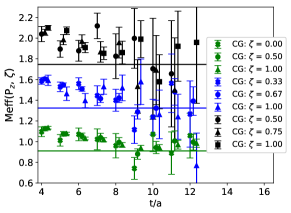
For pion momenta of about $1$ GeV or larger the two point functions is very noisy. To improve the signal following Ref. [12] we use boosted sources, where the valence quarks are boosted to momentum $\vec{k}=\zeta\vec{P}$, with $\vec{P}$ being the pion momentum and $\zeta$ is some number. Naively one would expect that the optimal choice is $\zeta=0.5$. In Figure 1 we show the effective masses for boosted Coulomb gauge Gaussian sources for different values of $\zeta$ at momentum 0.86 GeV, 1.29 GeV, and 1.72 GeV. At momentum 0.86 GeV we see significant improvement for both $\zeta=0.5$ and $\zeta=1.0$. At 1.29 GeV the non-boosted sources are very noisy and are not shown in the figure. Furthermore, $\zeta=1.0$ turns out to be too large while $\zeta=0.67$ yields the best results. At 1.72 GeV using $\zeta=0.5$ is not sufficient, while the choices $\zeta=0.75$ and $\zeta=1.00$ give similar results. It is clear, however, that even with boosted sources extracting the ground state at high momenta is difficult.

Next we performed two state fits for the pion correlation function

$$C_{\text{2pt}}(P_{z},t)=\sum_{i=1}^{2}2A_{i}e^{-\frac{1}{2}E_{i}T}\cosh{(E_{i}(T/2-t))},$$ (4)

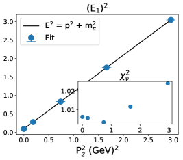
to obtain the energies of the ground state and the excited state for different momenta $P_{z}$. Here $T$ is the time extent of the lattice and $A_{i}=|\bra{i}\ket{\pi}|^{2}$. The results for the ground state energy as function of $P_{z}$ are shown in Figure 1. As one can see from the figure the determined energies follow the expected dispersion relation. In Table 1 we present the difference of the excited state energy with respect to the ground state energy for momenta 0 GeV, 0.86 GeV, 1.29 GeV, and 1.72 GeV. Interestingly, we find that this energy gap is approximately independent of $P_{z}$.

Table 1: The energy difference between first excited state and the ground state for different $P_{z}$.

$P_{z}$(N${}_{\text{cfg}}$)	0 GeV (52)	0.86 GeV (168)	1.29 GeV (168)	1.72 GeV (168)
$\Delta E_{2,1}$	1.39(38) GeV	1.26(04) GeV	1.15(08) GeV	1.32(36) GeV

Figure 1: Left: effective masses for different values of $\zeta$ with 50 configurations, Green, blue, and black points correspond to momentum 0.86, 1.29, and 1.72 GeV respectively. Right: the energy of the ground state as function of $P_{z}$ from the two state fit.

4 Calculations of Three-Point Function

To obtain the pion qPDF defined in Eq. (2) we consider the ratio of the three-point to the two point function

$$R(\Delta t,\tau,z;\Gamma)=\frac{\langle\pi(\vec{p},\Delta t)\mathcal{O}_{\Gamma}(z,\tau)\bar{\pi(0)}\rangle}{\langle\pi(\vec{p},\Delta t)\bar{\pi(0)}\rangle}=\frac{\sum_{n,n^{\prime}}A_{n}A_{n^{\prime}}^{*}e^{-E_{n}\Delta t}e^{-(E_{n^{\prime}}-E_{n})\tau}\bra{n}\mathcal{O}_{\Gamma}(z)\ket{n^{\prime}}}{\sum_{m}|A_{m}|^{2}e^{-E_{m}\Delta t}}$$ (5)

where $A_{n}=\bra{\pi}\ket{n}$,

$$\mathcal{O}_{\Gamma}(z)=\bar{\psi}(z)\Gamma W_{L}(z,0)\psi(0),$$ (6)

$\Delta t$ is the source-sink separation, and $\tau$ is the operator insertion time, such that $0<\tau<\Delta t$. For large $\Delta t$ and $\tau$ the above ratio gives the qPDF. Inserting a complete set of states and truncating the sum to the two lowest terms we write

$$R(\Delta t,\tau,z;\Gamma)\sim\frac{\mathscr{M}(z)+\mathscr{A}(z)e^{-\Delta E_{2,1}\tau}+\mathscr{A}^{\dagger}(z)e^{-\Delta E_{2,1}(\Delta t-\tau)}+\mathscr{B}(z)e^{-\Delta E_{2,1}\Delta t}+...}{1+\mathscr{C}e^{-\Delta E_{2,1}\Delta t}+...}.$$ (7)

Here, $\mathscr{M}(z)=\bra{1}\mathcal{O}_{\Gamma}(z)\ket{1}$ is the desired quantity, $\mathscr{A}(z)=\frac{A_{1}A_{2}^{*}}{|A_{1}|^{2}}\bra{1}\mathcal{O}_{\Gamma}(z)\ket{2}$, $\mathscr{B}(z)=\mathscr{C}\bra{2}\mathcal{O}_{\Gamma}(z)\ket{2}$, and $\mathscr{C}=\frac{|A_{2}|^{2}}{|A_{1}|^{2}}$.

In order to improve the signal we used one level of HYP smearing in the Wilson line entering Eq. (6). The ratio $R(\Delta t,\tau,z;\Gamma)$ obtained with one level of HYP smearing is larger compared to the unsmeared case. This is expected as smearing reduces the size of the self energy divergence in the Wilson line, see e.g. Ref. [13]. To obtain PDF one can use $\Gamma=\gamma_{t}$ or $\gamma_{z}$. The choice $\Gamma=\gamma_{t}$ has the advantage that in this case there is no mixing with the quark bilinear operator with $\Gamma=1$ [4]. It also turns out that excited state contamination is smaller for $\Gamma=\gamma_{t}$. In what follows we discuss the calculations using one level of HYP smearing and $\Gamma=\gamma_{t}$.

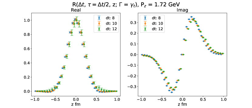
In Figure 2 we show the z dependence of $R(\Delta t,\tau,z;\gamma_{t})$ for three source sink separations, $\Delta t=8,~{}10$ and $12$, and $\tau=\Delta t/2$. The data points have been shifted horizontally for better visibility. We see a weak dependence on $\Delta t$ indicating that the contribution of the excited states to $R(\Delta t,\tau,z;\gamma_{t})$ is small. To extract the ground-state quasi-PDF matrix element we employ two fitting procedures used in Refs. [14, 15].

Figure 2: $R(\Delta t,\tau,z;\gamma_{t})$ at $P_{z}=1.72$ GeV as function of $z$ for $\Delta t/a=$ 8 (blue), 10 (orange), and 12 (green) and $\tau=\Delta t/2$.

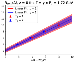
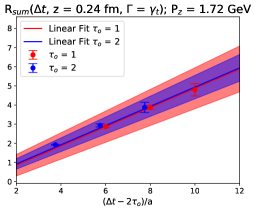
First we use the summation method [15]. Here one sums over all $\tau$ minus a certain number of end points $\tau_{o}$

$$R_{\text{sum}}(\Delta t,z;\Gamma)=\sum_{\tau=\tau_{o}}^{\Delta t-\tau_{o}}R(\Delta t,\tau,z;\Gamma)\sim(\mathscr{M}+\mathscr{B}e^{-\Delta E_{2,1}\Delta t})(\Delta t-2\tau_{o})+const.$$ (8)

We calculate $R_{\text{sum}}(\Delta t,z;\Gamma)$ according to the above equation and then perform a linear fit with respect to $\Delta t-2\tau_{o}$. The slope obtained from the fit gives $\mathscr{M}$ for large enough $\Delta t$. In Fig. 3 we show the results of the summation method for $z=0$ fm and $z=0.24$ fm and $P_{z}=1.72$ GeV using $\tau_{o}=1$ and $\tau_{o}=2$. For both values of $z$ the choice $\tau_{o}=2$ gives the most precise result.

Figure 3: $R_{\text{sum}}$ at $P_{z}=1.72$ GeV as function of $\Delta t-2\tau_{o}$ for $z=0$ (left) and $z=0.24$ fm (right). The lines show the fit results and the bands show the corresponding uncertainty. Red and blue data points and bands are for results with $\tau_{o}$ = 1 and $\tau_{o}$ = 2 respectively.

The second method relies on simultaneous fit of the $\Delta t$ and $\tau$ dependence of the ratio $R(\Delta t,\tau,z;\gamma_{t})$ to the form given by Eq. (7), which we refer to as the two-state fit [14]. Here we use $\Delta E_{2,1}$ obtained from the two-point correlator and summarized in Table 1 and treat $\mathscr{M}$, $\mathscr{A}$, and $\mathscr{B}$ as fit parameters.

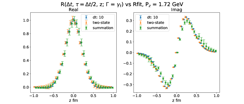
In Fig. 4 we show our results for $\mathscr{M}$ obtained using the summation method and two-state fit. We also compare $\mathscr{M}$ with the $R(\Delta t,\tau,z;\gamma_{t})$ evaluated at $\Delta t$ = 10 with the $\tau=\Delta t/2$. For the real part the two methods extracting $\mathscr{M}$ agree within errors and also agree with $R(\Delta t=10,\tau=5,z;\gamma_{t})$. This means that excited state contributions are under control. The imaginary part of $\mathscr{M}$ obtained with the summation method does differ somewhat to the results with two-state fit and ${\rm Im}R(\Delta t/a=10,\tau/a=5,z;\gamma_{t})$, meaning that excited states have some effects in the imaginary part.

Figure 4: The real part (left) and the imaginary part (right) of $\mathscr{M}$ for $P_{z}=1.72$ GeV. obtained using the summation method and the two-state fit. We also show our results for $R(\Delta t/a=10,\tau/a=5,z;\gamma_{t})$.

5 Calculating the parton distribution

The matrix element $\mathscr{M}$ that defines the qPDF needs to be renormalized. We perform the renormalization using regularization independent momentum subtraction (RI-MOM) scheme. To define the renormalization constant one calculates the expectation value of the non-local quark bilinear in Eq. (6) on off-shell quark states: $\Lambda(p,z)=\bra{p}O_{\gamma_{t}}(z)\ket{p}$. The renormalization condition is defined such that the renormalized matrix element $\Lambda^{R}(p,z)=Z(z,p_{z}^{R},p^{R})\Lambda(p,z)$ satisfies the condition ${\rm Tr}\not{p}\Lambda^{R}(p,z)|_{p=p^{R}}=12p_{t}^{R}exp(-ip_{z}^{R}z)$, i.e. it equals to the tree level result for $p=p_{R}$. The RI-MOM scheme here depends on two renormalization scales: $p_{z}^{R}$ and $p_{R}^{2}=(p_{z}^{R})^{2}+(p_{\perp}^{R})^{2}$, because the $z$ direction plays a special role. In other words, for RI-MOM scheme $\mu_{L}=\{p_{z}^{R},p_{R}^{2}\}$. A more detailed discussion of our RI-MOM renormalization procedure is given in Ref. [16]. Multiplying the bare matrix element by $Z(z,p_{z}^{R},p_{R}^{2})$ we get the renormalized matrix element $\mathscr{M}^{R}$, which then can be used to calculate the qPDF according to Eq. (2). In our preliminary study we used $R(\Delta t/a=10,\tau/a=5,z;\gamma_{t})$ as proxy for $\mathscr{M}$. As discussed in the previous section the excited state contamination is small for $\Delta t/a=10$. To perform the Fourier transformation in Eq. (2) we need to information about $\mathscr{M}^{R}$ for all $z$. However, our numerical calculations only cover the value of $|z|$ up to $1$ fm. Since $\mathscr{M}^{R}$ decays rapidly at large $z$ we assume that it vanishes for $|z/a|=20$ and perform interpolation of the lattice results on $\mathscr{M}^{R}$ with this constraint. Using this interpolation we calculate the qPDF $\tilde{q}(x,P_{z},p_{z}^{R},p_{R})$ [16]. The resulting qPDF are shown in Fig. 5 as dashed lines. We checked that the numerical results do not change much if we assume that the coordinate space qPDF vanishes at $|z/a|=24$.

Figure 5: Left: PDF and qPDF for different values of $P_{z}$. Right: the dependence of PDF and qPDF on the RI-MOM renormalizations scales for $P_{z}=1.72$ GeV.

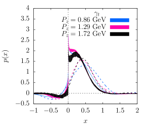
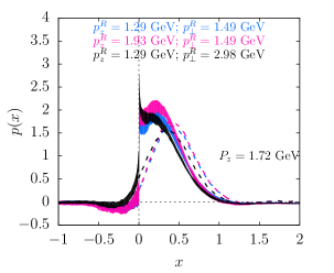
To calculate PDF from qPDF we invert Eq. (3) to leading order in $\alpha_{s}$. The matching kernel $C$ entering Eq. (3) for $\Gamma=\gamma_{t}$ and qPDF in RI-MOM scheme has been calculated at 1-loop in Ref. [5], and we make use of the corresponding result in our analysis. Our results for pion PDF are shown in Fig. 5. We see that for $P_{z}\geq 1.29$ GeV the dependence of the reconstructed PDF on $P_{z}$ is very small. The PDF should be independent on RI-MOM scale parameters $p_{z}^{R}$ and $p_{R}^{2}$ because this dependence cancels out between qPDF and the matching kernel $C$. In practice, however, this cancellation is not exact as the matching kernel is only know at 1-loop. From Fig. 5 we see that the dependence on $p_{z}^{R}$ and $p^{R}$ is rather mild, which is encouraging and indicates that the outlined strategy for calculating PDF is viable.

6 Conclusions

In this contribution we presented preliminary calculations of quark distribution inside the pion from lattice QCD based on Large Momentum Effective Theory approach by Ji. We used fine lattices ($a=0.06$fm) in order to utilize the pertubative matching between qPDF and PDF. To obtain the renormalized qPDF we used the non-perturbative RI-MOM scheme. Obtaining the ground state signal for the fast moving pion is very challenging and in order to reach this goal we used momentum boosted sources. With these we were able to reach pion momenta up to $1.72$ GeV. In order to perform calculations at even larger values of $P_{z}$ significantly more statistics will be needed.