Generalized Symmetric ADMM for Separable Convex Optimization

Abstract

The Alternating Direction Method of Multipliers (ADMM) has been proved to be effective for solving separable convex optimization subject to linear constraints. In this paper, we propose a Generalized Symmetric ADMM (GS-ADMM), which updates the Lagrange multiplier twice with suitable stepsizes, to solve the multi-block separable convex programming. This GS-ADMM partitions the data into two group variables so that one group consists of $p$ block variables while the other has $q$ block variables, where $p\geq 1$ and $q\geq 1$ are two integers. The two grouped variables are updated in a Gauss-Seidel scheme, while the variables within each group are updated in a Jacobi scheme, which would make it very attractive for a big data setting. By adding proper proximal terms to the subproblems, we specify the domain of the stepsizes to guarantee that GS-ADMM is globally convergent with a worst-case ${\cal{O}}(1/t)$ ergodic convergence rate. It turns out that our convergence domain of the stepsizes is significantly larger than other convergence domains in the literature. Hence, the GS-ADMM is more flexible and attractive on choosing and using larger stepsizes of the dual variable. Besides, two special cases of GS-ADMM, which allows using zero penalty terms, are also discussed and analyzed. Compared with several state-of-the-art methods, preliminary numerical experiments on solving a sparse matrix minimization problem in the statistical learning show that our proposed method is effective and promising.

1 Introduction

We consider the following grouped multi-block separable convex programming problem

$$\begin{array}[]{lll}\min&\sum\limits_{i=1}^{p}f_{i}(x_{i})+\sum\limits_{j=1}^{q}g_{j}(y_{j})\\ \textrm{s.t. }&\sum\limits_{i=1}^{p}A_{i}x_{i}+\sum\limits_{j=1}^{q}B_{j}y_{j}=c,\\ &x_{i}\in\mathcal{X}_{i},\;i=1,\cdots,p,\\ &y_{j}\in\mathcal{Y}_{j},\;j=1,\cdots,q,\\ \end{array}$$ (1)

where $f_{i}(x_{i}):\mathcal{R}^{m_{i}}\rightarrow\mathcal{R},\ g_{j}(y_{j}):\mathcal{R}^{d_{j}}\rightarrow\mathcal{R}$ are closed and proper convex functions (possibly nonsmooth); $A_{i}\in\mathcal{R}^{n\times m_{i}},B_{j}\in\mathcal{R}^{n\times d_{j}}$ and $c\in\mathcal{R}^{n}$ are given matrices and vectors, respectively; $\mathcal{X}_{i}\subset\mathcal{R}^{m_{i}}$ and $\mathcal{Y}_{j}\subset\mathcal{R}^{d_{j}}$ are closed convex sets; $p\geq 1$ and $q\geq 1$ are two integers. Throughout this paper, we assume that the solution set of the problem (1) is nonempty and all the matrices $A_{i}$, $i=1,\cdots,p$, and $B_{j}$, $j=1,\cdots,q$, have full column rank. And in the following, we denote $\mathcal{A}=\left(A_{1},\cdots,A_{p}\right),\mathcal{B}=\left(B_{1},\cdots,B_{q}\right)$, ${\bf{x}}=(x_{1}^{\sf T},\cdots,x_{p}^{\sf T})^{\sf T}$, ${\bf{y}}=(y_{1}^{\sf T},\cdots,y_{q}^{\sf T})^{\sf T}$, ${\cal{X}}={\cal{X}}_{1}\times{\cal{X}}_{2}\times\cdots{\cal{X}}_{p}$, ${\cal{Y}}={\cal{Y}}_{1}\times{\cal{Y}}_{2}\times\cdots{\cal{Y}}_{q}$ and $\mathcal{M}=\mathcal{X}\times\mathcal{Y}\times\mathcal{R}^{n}$.

In the last few years, the problem (1) has been extensively investigated due to its wide applications in different fields, such as the sparse inverse covariance estimation problem RothmanBickel2008 in finance and statistics, the model updating problem DongYuTian2015 in the design of vibration structural dynamic system and bridges, the low rank and sparse representations LiuLiBai2017 in image processing and so forth. One standard way to solve the problem (1) is the classical Augmented Lagrangian Method (ALM) Hestenes1969 , which minimizes the following augmented Lagrangian function

$$\mathcal{L}_{\beta}\left({\bf{x}},{\bf{y}},\lambda\right)=L\left({\bf{x}},{\bf{y}},\lambda\right)+\frac{\beta}{2}\|{\cal{A}}{\bf{x}}+{\cal{B}}{\bf{y}}-c\|^{2},$$

where $\beta>0$ is a penalty parameter for the equality constraint and

$$L\left({\bf{x}},{\bf{y}},\lambda\right)=\sum\limits_{i=1}^{p}f_{i}(x_{i})+\sum\limits_{j=1}^{q}g_{j}(y_{j})-\langle\lambda,{\cal{A}}{\bf{x}}+{\cal{B}}{\bf{y}}-c\rangle$$ (2)

is the Lagrangian function of the problem (1) with the Lagrange multiplier $\lambda\in\mathcal{R}^{n}$. Then, the ALM procedure for solving (1) can be described as follows:

$$\left\{\begin{array}[]{l}\left({\bf{x}}^{k+1},{\bf{y}}^{k+1}\right)=\arg\min\left\{\mathcal{L}_{\beta}\left({\bf{x}},{\bf{y}},\lambda^{k}\right)|\ {\bf{x}}\in\mathcal{X},{\bf{y}}\in\mathcal{Y}\right\},\\ \lambda^{k+1}=\lambda^{k}-\beta({\cal{A}}{\bf{x}}^{k+1}+{\cal{B}}{\bf{y}}^{k+1}-c).\end{array}\right.$$

However, ALM does not make full use of the separable structure of the objective function of (1) and hence, could not take advantage of the special properties of the component objective functions $f_{i}$ and $g_{j}$ in (1). As a result, in many recent real applications involving big data, solving the subproblems of ALM becomes very expensive.

One effective approach to overcome such difficulty is the Alternating Direction Method of Multipliers (ADMM), which was originally proposed in GlowinskiMarrocco1975 and could be regarded as a splitting version of ALM. At each iteration, ADMM first sequentially optimize over one block variable while fixing all the other block variables, and then follows by updating the Lagrange multiplier. A natural extension of ADMM for solving the multi-block case problem (1) takes the following iterations:

$$\left\{\begin{array}[]{lll}\textrm{For}\ i=1,2,\cdots,p,\\ \qquad x_{i}^{k+1}=\arg\min\limits_{x_{i}\in\mathcal{X}_{i}}\mathcal{L}_{\beta}\left(x_{1}^{k+1},\cdots,x_{i-1}^{k+1},x_{i},x_{i+1}^{k},\cdots,x_{p}^{k},{\bf{y}}^{k},\lambda^{k}\right),\\ \textrm{For}\ j=1,2,\cdots,q,\\ \qquad y_{j}^{k+1}=\arg\min\limits_{y_{j}\in\mathcal{Y}_{j}}\mathcal{L}_{\beta}\left({\bf{x}}^{k+1},y_{1}^{k+1},\cdots,y_{j-1}^{k+1},y_{j},y_{j+1}^{k},\cdots,y_{q}^{k},\lambda^{k}\right),\\ \lambda^{k+1}=\lambda^{k}-\beta\left(\mathcal{A}{\bf{x}}^{k+1}+\mathcal{B}{\bf{y}}^{k+1}-c\right).\end{array}\right.$$ (3)

Obviously, the scheme (3) is a serial algorithm which uses the newest information of the variables at each iteration. Although the above scheme was proved to be convergent for the two-block, i.e., $p=q=1$, separable convex minimization (see HeYuan2012 ), as shown in Chen2016 , the direct extension of ADMM (3) for the multi-block case, i.e., $p+q\geq 3$, without proper modifications is not necessarily convergent. Another natural extension of ADMM is to use the Jacobian fashion, where the variables are updated simultaneously after each iteration, that is,

$$\left\{\begin{array}[]{lll}\textrm{For}\ i=1,2,\cdots,p,\\ \qquad x_{i}^{k+1}=\arg\min\limits_{x_{i}\in\mathcal{X}_{i}}\mathcal{L}_{\beta}\left(x_{1}^{k},\cdots,x_{i-1}^{k},x_{i},x_{i+1}^{k},\cdots,x_{p}^{k},{\bf{y}}^{k},\lambda^{k}\right),\\ \textrm{For}\ j=1,2,\cdots,q,\\ \qquad y_{j}^{k+1}=\arg\min\limits_{y_{j}\in\mathcal{Y}_{j}}\mathcal{L}_{\beta}\left({\bf{x}}^{k},y_{1}^{k},\cdots,y_{j-1}^{k},y_{j},y_{j+1}^{k},\cdots,y_{q}^{k},\lambda^{k}\right),\\ \lambda^{k+1}=\lambda^{k}-\beta\left(\mathcal{A}{\bf{x}}^{k+1}+\mathcal{B}{\bf{y}}^{k+1}-c\right).\end{array}\right.$$ (4)

As shown in HeHouYuan2015 , however, the Jacobian scheme (4) is not necessarily convergent either. To ensure the convergence, He et al. HeTaoYuan2015 proposed a novel ADMM-type splitting method that by adding certain proximal terms, allowed some of the subproblems to be solved in parallel, i.e., in a Jacobian fashion. And in HeTaoYuan2015 , some sparse low-rank models and image painting problems were tested to verify the efficiency of their method.

More recently, a Symmetric ADMM (S-ADMM) was proposed by He et al. HeMaYuan2016 for solving the two-block separable convex minimization, where the algorithm performs the following updating scheme:

$$\left\{\begin{array}[]{lll}{\bf{x}}^{k+1}=\arg\min\left\{\mathcal{L}_{\beta}\left({\bf{x}},{\bf{y}}^{k},\lambda^{k}\right)\ |\ {\bf{x}}\in\mathcal{X}\right\},\\ \lambda^{k+\frac{1}{2}}=\lambda^{k}-\tau\beta\left({\cal{A}}{\bf{x}}^{k+1}+{\cal{B}}{\bf{y}}^{k}-c\right),\\ {\bf{y}}^{k+1}=\arg\min\left\{\mathcal{L}_{\beta}({\bf{x}}^{k+1},{\bf{y}},\lambda^{k+\frac{1}{2}})\ |\ {\bf{y}}\in\mathcal{Y}\right\},\\ \lambda^{k+1}=\lambda^{k+\frac{1}{2}}-s\beta\left({\cal{A}}{\bf{x}}^{k+1}+{\cal{B}}{\bf{y}}^{k+1}-c\right),\end{array}\right.$$ (5)

and the stepsizes $(\tau,s)$ were restricted into the domain

$$\mathcal{H}=\left\{(\tau,s)\ |\ s\in(0,(\sqrt{5}+1)/2),\ \tau+s>0,\ \tau\in(-1,1),\ |\tau|<1+s-s^{2}\right\}$$ (6)

in order to ensure its global convergence. The main improvement of HeMaYuan2016 is that the scheme (5) largely extends the domain of the stepsizes $(\tau,s)$ of other ADMM-type methods HeLiuWangYuan2014 . What’s more, the numerical performance of S-ADMM on solving the widely used basis pursuit model and the total-variational image debarring model significantly outperforms the original ADMM in both the CPU time and the number of iterations. Besides, Gu, et al.GuJiang2015 also studied a semi-proximal-based strictly contractive Peaceman-Rachford splitting method, that is (5) with two additional proximal penalty terms for the $x$ and $y$ update. But their method has a nonsymmetric convergence domain of the stepsize and still focuses on the two-block case problem, which limits its applications for solving large-scale problems with multiple block variables.

Mainly motivated by the work of HeTaoYuan2015 ; HeMaYuan2016 ; GuJiang2015 , we would like to generalize S-ADMM with more wider convergence domain of the stepsizes to tackle the multi-block separable convex programming model (1), which more frequently appears in recent applications involving big data Chandrasekaran2012 ; Ma2017 . Our algorithm framework can be described as follows:

$$(\textbf{GS-ADMM})\ \left\{\begin{array}[]{lll}\textrm{For}\ i=1,2,\cdots,p,\\ \quad x_{i}^{k+1}=\arg\min\limits_{x_{i}\in\mathcal{X}_{i}}\mathcal{L}_{\beta}(x_{1}^{k},\cdots,x_{i},\cdots,x_{p}^{k},{\bf{y}}^{k},\lambda^{k})+P_{i}^{k}(x_{i}),\\ \quad\textrm{where }P_{i}^{k}(x_{i})=\frac{\sigma_{1}\beta}{2}\left\|A_{i}(x_{i}-x_{i}^{k})\right\|^{2},\\ \lambda^{k+\frac{1}{2}}=\lambda^{k}-\tau\beta(\mathcal{A}{\bf{x}}^{k+1}+\mathcal{B}{\bf{y}}^{k}-c),\\ \\ \textrm{For}\ j=1,2,\cdots,q,\\ \quad y_{j}^{k+1}=\arg\min\limits_{y_{j}\in\mathcal{Y}_{j}}\mathcal{L}_{\beta}({\bf{x}}^{k+1},y_{1}^{k},\cdots,y_{j},\cdots,y_{q}^{k},\lambda^{k+\frac{1}{2}})+Q_{j}^{k}(y_{j}),\\ \quad\textrm{where }Q_{j}^{k}(y_{j})=\frac{\sigma_{2}\beta}{2}\left\|B_{j}(y_{j}-y_{j}^{k})\right\|^{2},\\ \lambda^{k+1}=\lambda^{k+\frac{1}{2}}-s\beta(\mathcal{A}{\bf{x}}^{k+1}+\mathcal{B}{\bf{y}}^{k+1}-c).\end{array}\right.$$ (7)

In the above Generalized Symmetric ADMM (GS-ADMM), $\tau$ and $s$ are two stepsize parameters satisfying

$$(\tau,s)\in{\cal{K}}=\left\{(\tau,s)\ |\ \tau+s>0,\ \tau\leq 1,\ -\tau^{2}-s^{2}-\tau s+\tau+s+1>0\right\},$$ (8)

and $\sigma_{1}\in(p-1,+\infty),\sigma_{2}\in(q-1,+\infty)$ are two proximal parameters for the regularization terms $P_{i}^{k}(\cdot)$ and $Q_{j}^{k}(\cdot)$. He and YuanHeyuan2015 also investigated the above GS-ADMM (7) but restricted the stepsize $\tau=s\in(0,1)$, which does not exploit the advantages of using flexible stepsizes given in (8) to improve its convergence.

Fig 1. Stepsize region $\mathcal{K}$ of GS-ADMM

Major contributions of this paper can be summarized as the following four aspects:

• Firstly, the new GS-ADMM could deal with the multi-block separable convex programming problem (1), while the original S-ADMM in HeMaYuan2016 only works for the two block case and may not be convenient for solving large-scale problems. In addition, the convergence domain $\mathcal{K}$ for the stepsizes $(\tau,s)$ in (8), shown in Fig. 1, is significantly larger than the domain $\mathcal{H}$ given in (6) and the convergence domain in GuJiang2015 ; Heyuan2015 . For example, the stepsize $s$ can be arbitrarily close to $5/3$ when the stepsize $\tau$ is close to $-1/3$. Moreover, the above domain in (8) is later enlarged to a symmetric domain ${\cal{G}}$ defined in (112), shown in Fig. 2. Numerical experiments in Sec. 5.2.1 also validate that using more flexible and relatively larger stepsizes $(\tau,s)$ can often improve the convergence speed of GS-ADMM. On the other hand, we can see that when $\tau=0$, the stepsize $s$ can be chosen in the interval $(0,(\sqrt{5}+1)/2)$, which was firstly suggested by Fortin and Glowinski in FortinGlowinski1983 ; Glowinski1984 .

• Secondly, the global convergence of GS-ADMM as well as its worst-case ${\cal{O}}(1/t)$ ergodic convergence rate are established. What’s more, the total $p+q$ block variables are partitioned into two grouped variables. While a Gauss-Seidel fashion is taken between the two grouped variables, the block variables within each group are updated in a Jacobi scheme. Hence, parallel computing can be implemented for updating the variables within each group, which could be critical in some scenarios for problems involving big data.

• Thirdly, we discuss two special cases of GS-ADMM, which is (7) with $p\geq 1,q=1$ and $\sigma_{2}=0$ or with $p=1,q\geq 1$ and $\sigma_{1}=0$. These two special cases of GS-ADMM were not discussed in Heyuan2015 and in fact, to the best of our knowledge, they have not been studied in the literature. We show the convergence domain of the stepsizes $(\tau,s)$ for these two cases is still ${\cal{K}}$ defined in (8) that is larger than $\mathcal{H}$.

• Finally, numerical experiments are performed on solving a sparse matrix optimization problem arising from the statistical learning. We have investigated the effects of the stepsizes $(\tau,s)$ and the penal parameter $\beta$ on the performance of GS-ADMM. And our numerical experiments demonstrate that by properly choosing the parameters, GS-ADMM could perform significantly better than other recently quite popular methods developed in BaiLiLi2017 ; HeTaoYuan2015 ; HeXuYuan2016 ; WangSong2017 .

The paper is organized as follows. In Section 2, some preliminaries are given to reformulate the problem (1) into a variational inequality and to interpret the GS-ADMM (7) as a prediction-correction procedure. Section 3 investigates some properties of $\|{\bf{w}}^{k}-{\bf{w}}^{*}\|_{H}^{2}$ and provides a lower bound of $\|{\bf{w}}^{k}-\widetilde{{\bf{w}}}^{k}\|_{G}^{2}$, where $H$ and $G$ are some particular symmetric matrices. Then, we establish the global convergence of GS-ADMM and show its convergence rate in an ergodic sense. In Section 4, we discuss two special cases of GS-ADMM, in which either the penalty parameters $\sigma_{1}$ or $\sigma_{2}$ is allowed to be zero. Some preliminary numerical experiments are done in Section 5. We finally make some conclusions in Section 6.

1.1 Notation

Denoted by $\mathcal{R},\mathcal{R}^{n},\mathcal{R}^{m\times n}$ be the set of real numbers, the set of $n$ dimensional real column vectors and the set of $m\times n$ real matrices, respectively. For any $x,y\in\mathcal{R}^{n}$, $\langle x,y\rangle=x^{\sf T}y$ denotes their inner product and $\|x\|=\sqrt{\langle x,x\rangle}$ denotes the Euclidean norm of $x$, where the superscript ^T is the transpose. Given a symmetric matrix $G$, we define $\|x\|_{G}^{2}=x^{\sf T}Gx$. Note that with this convention, $\|x\|_{G}^{2}$ is not necessarily nonnegative unless $G$ is a positive definite matrix ($\succeq\textbf{0}$). For convenience, we use $I$ and $\bf{0}$ to stand respectively for the identity matrix and the zero matrix with proper dimension throughout the context.

2 Preliminaries

In this section, we first use a variational inequality to characterize the solution set of the problem (1). Then, we analyze that GS-ADMM (7) can be treated as a prediction-correction procedure involving a prediction step and a correction step.

2.1 Variational reformulation of (1)

We begin with the following standard lemma whose proof can be found in HeMaYuan2016 ; He2016 .

Lemma 1

Let $f:\mathcal{R}^{m}\longrightarrow\mathcal{R}$ and $h:\mathcal{R}^{m}\longrightarrow\mathcal{R}$ be two convex functions defined on a closed convex set $\Omega\subset\mathcal{R}^{m}$ and $h$ is differentiable. Suppose that the solution set $\Omega^{*}=\arg\min\limits_{x\in\Omega}\{f(x)+h(x)\}$ is nonempty. Then, we have

$$x^{*}\in\Omega^{*}\ \mbox{ if and only if }\ x^{*}\in\Omega,\ f(x)-f(x^{*})+\left\langle x-x^{*},\nabla h(x^{*})\right\rangle\geq 0,\forall x\in\Omega.$$

It is well-known in optimization that a triple point $({\bf{x}}^{*},{\bf{y}}^{*},\lambda^{*})\in{\cal{M}}$ is called the saddle-point of the Lagrangian function (2) if it satisfies

$$L\left({\bf{x}}^{*},{\bf{y}}^{*},\lambda\right)\leq L\left({\bf{x}}^{*},{\bf{y}}^{*},\lambda^{*}\right)\leq L\left({\bf{x}},{\bf{y}},\lambda^{*}\right),\quad\forall({\bf{x}},{\bf{y}},\lambda)\in\mathcal{M}$$

which can be also characterized as

$$\left\{\begin{array}[]{lll}\textrm{For}\ i=1,2,\cdots,p,\\ \qquad x_{i}^{*}=\arg\min\limits_{x_{i}\in\mathcal{X}_{i}}\mathcal{L}_{\beta}\left(x_{1}^{*},\cdots,x_{i-1}^{*},x_{i},x_{i+1}^{*},\cdots,x_{p}^{*},{\bf{y}}^{*},\lambda^{*}\right),\\ \textrm{For}\ j=1,2,\cdots,q,\\ \qquad y_{j}^{*}=\arg\min\limits_{y_{j}\in\mathcal{Y}_{j}}\mathcal{L}_{\beta}\left({\bf{x}}^{*},y_{1}^{*},\cdots,y_{j-1}^{*},y_{j},y_{j+1}^{*},\cdots,y_{q}^{*},\lambda^{*}\right),\\ \lambda^{*}=\arg\max\limits_{\lambda\in\mathcal{R}^{n}}\mathcal{L}_{\beta}\left({\bf{x}}^{*},{\bf{y}}^{*},\lambda\right).\end{array}\right.$$

Then, by Lemma 1, the above saddle-point equations can be equivalently expressed as

$$\left\{\begin{array}[]{lll}\textrm{For}\ i=1,2,\cdots,p,\\ \qquad x_{i}^{*}\in\mathcal{X}_{i},\quad f_{i}(x_{i})-f_{i}(x_{i}^{*})+\langle x_{i}-x_{i}^{*},-A_{i}^{\sf T}\lambda^{*}\rangle\geq 0,\forall x_{i}\in\mathcal{X}_{i},\\ \textrm{For}\ j=1,2,\cdots,q,\\ \qquad y_{j}^{*}\in\mathcal{Y}_{j},\quad g_{j}(y_{j})-g_{j}(y_{j}^{*})+\langle y_{j}-y_{j}^{*},-B_{j}^{\sf T}\lambda^{*}\rangle\geq 0,\forall y_{j}\in\mathcal{Y}_{j},\\ \lambda^{*}\in\mathcal{R}^{n},\quad\left\langle\lambda-\lambda^{*},{\cal{A}}{\bf{x}}^{*}+{\cal{B}}{\bf{y}}^{*}-c\right\rangle\geq 0,\forall\lambda\in\mathcal{R}^{n}.\end{array}\right.$$ (9)

Rewriting (9) in a more compact variational inequality (VI) form, we have

$$h({\bf{u}})-h({\bf{u}}^{*})+\left\langle{\bf{w}}-{\bf{w}}^{*},\mathcal{J}({\bf{w}}^{*})\right\rangle\geq 0,\quad\forall{\bf{w}}\in\mathcal{M},$$ (10)

where

$$h({\bf{u}})=\sum_{i=1}^{p}f_{i}(x_{i})+\sum_{j=1}^{p}g_{j}(y_{j})$$

and

$${\bf{u}}=\left(\begin{array}[]{c}{\bf{x}}\\ {\bf{y}}\\ \end{array}\right),\quad{\bf{w}}=\left(\begin{array}[]{c}{\bf{x}}\\ {\bf{y}}\\ \lambda\end{array}\right),\quad\mathcal{J}({\bf{w}})=\left(\begin{array}[]{c}-{\cal{A}}^{\sf T}\lambda\\ -{\cal{B}}^{\sf T}\lambda\\ {\cal{A}}{\bf{x}}+{\cal{B}}{\bf{y}}-c\end{array}\right).$$

Noticing that the affine mapping ${\cal{J}}$ is skew-symmetric, we immediately get

$$\left\langle{\bf{w}}-\widehat{{\bf{w}}},\mathcal{J}({\bf{w}})-\mathcal{J}(\widehat{{\bf{w}}})\right\rangle=0,\quad\forall\ {\bf{w}},\widehat{{\bf{w}}}\in\mathcal{M}.$$ (11)

Hence, (10) can be also rewritten as

$$\textrm{VI}({\bf{h}},\mathcal{J},\mathcal{M}):\quad h({\bf{u}})-h({\bf{u}}^{*})+\left\langle{\bf{w}}-{\bf{w}}^{*},\mathcal{J}({\bf{w}})\right\rangle\geq 0,\quad\forall{\bf{w}}\in\mathcal{M}.$$ (12)

Because of the nonempty assumption on the solution set of (1), the solution set $\mathcal{M}^{*}$ of the variational inequality $\textrm{VI}(h,\mathcal{J},\mathcal{M})$ is also nonempty and convex, see e.g. Theorem 2.3.5 FacchineiPang2003 for more details. The following theorem given by Theorem 2.1 HeYuan2012 provides a concrete way to characterize the set $\mathcal{M}^{*}$.

Theorem 2.1

The solution set of the variational inequality $\textrm{VI}(h,\mathcal{J},\mathcal{M})$ is convex and can be expressed as

$$\mathcal{M}^{*}=\bigcap_{{\bf{w}}\in\mathcal{M}}\left\{\widehat{{\bf{w}}}\in\mathcal{M}|\ h({\bf{u}})-h(\widehat{{\bf{u}}})+\left\langle{\bf{w}}-\widehat{{\bf{w}}},\mathcal{J}({\bf{w}})\right\rangle\geq 0\right\}.$$

2.2 A prediction-correction interpretation of GS-ADMM

Following a similar approach in HeMaYuan2016 , we next interpret GS-ADMM as a prediction-correction procedure. First, let

$$\widetilde{{\bf{x}}}^{k}=\left(\begin{array}[]{c}\widetilde{x}_{1}^{k}\\ \widetilde{x}_{2}^{k}\\ \vdots\\ \widetilde{x}_{p}^{k}\end{array}\right)=\left(\begin{array}[]{c}x_{1}^{k+1}\\ x_{2}^{k+1}\\ \vdots\\ x_{p}^{k+1}\end{array}\right),\quad\widetilde{{\bf{y}}}^{k}=\left(\begin{array}[]{c}\widetilde{y}_{1}^{k}\\ \widetilde{y}_{2}^{k}\\ \vdots\\ \widetilde{y}_{q}^{k}\end{array}\right)=\left(\begin{array}[]{c}y_{1}^{k+1}\\ y_{2}^{k+1}\\ \vdots\\ y_{q}^{k+1}\end{array}\right),$$ (13)

$$\widetilde{\lambda}^{k}=\lambda^{k}-\beta\left(\mathcal{A}{\bf{x}}^{k+1}+\mathcal{B}{\bf{y}}^{k}-c\right),$$ (14)

and

$$\widetilde{{\bf{u}}}=\left(\begin{array}[]{c}\widetilde{{\bf{x}}}\\ \widetilde{{\bf{y}}}\\ \end{array}\right),\quad\widetilde{{\bf{w}}}^{k}=\left(\begin{array}[]{c}\widetilde{{\bf{x}}}^{k}\\ \widetilde{{\bf{y}}}^{k}\\ \widetilde{\lambda}^{k}\end{array}\right)=\left(\begin{array}[]{c}{\bf{x}}^{k+1}\\ {\bf{y}}^{k+1}\\ \widetilde{\lambda}^{k}\end{array}\right).$$ (15)

Then, by using the above notations, we derive the following basic lemma.

Lemma 2

For the iterates $\widetilde{{\bf{u}}}^{k},\widetilde{{\bf{w}}}^{k}$ defined in (15), we have $\widetilde{{\bf{w}}}^{k}\in\mathcal{M}$ and

$$h({\bf{u}})-h(\widetilde{{\bf{u}}}^{k})+\left\langle{\bf{w}}-\widetilde{{\bf{w}}}^{k},\mathcal{J}(\widetilde{{\bf{w}}}^{k})+Q(\widetilde{{\bf{w}}}^{k}-{\bf{w}}^{k})\right\rangle\geq 0,\quad\forall{\bf{w}}\in\mathcal{M},$$ (16)

where

$$Q=\left[\begin{array}[]{cc}H_{\mathbf{x}}&\bf{0}\\ \bf{0}&\widetilde{Q}\end{array}\right]$$ (17)

with

$$H_{\mathbf{x}}=\beta\left[\begin{array}[]{ccccccccccccc}\sigma_{1}A_{1}^{\sf T}A_{1}&&&&-A_{1}^{\sf T}A_{2}&&&&\cdots&&&&-A_{1}^{\sf T}A_{p}\\ \\ -A_{2}^{\sf T}A_{1}&&&&\sigma_{1}A_{2}^{\sf T}A_{2}&&&&\cdots&&&&-A_{2}^{\sf T}A_{p}\\ \\ \vdots&&&&\vdots&&&&\ddots&&&&\vdots\\ \\ -A_{p}^{\sf T}A_{1}&&&&-A_{p}^{\sf T}A_{2}&&&&\cdots&&&&\sigma_{1}A_{p}^{\sf T}A_{p}\end{array}\right],$$ (18)

$$\widetilde{Q}=\left[\begin{array}[]{ccccccccccccccc|cc}(\sigma_{2}+1)\beta B_{1}^{\sf T}B_{1}&&&&{\bf 0}&&&&\cdots&&&&{\bf 0}&&&&-\tau B_{1}^{\sf T}\\ &&&&&&&&&&&&&&&&\\ {\bf 0}&&&&(\sigma_{2}+1)\beta B_{2}^{\sf T}B_{2}&&&&\cdots&&&&{\bf 0}&&&&-\tau B_{2}^{\sf T}\\ &&&&&&&&&&&&&&&&\\ \vdots&&&&\vdots&&&&\ddots&&&&\vdots&&&&\vdots\\ &&&&&&&&&&&&&&&&\\ {\bf 0}&&&&{\bf 0}&&&&\cdots&&&&(\sigma_{2}+1)\beta B_{q}^{\sf T}B_{q}&&&&-\tau B_{q}^{\sf T}\\ &&&&&&&&&&&&&&&&\\ \hline\cr-B_{1}&&&&-B_{2}&&&&\cdots&&&&-B_{q}&&&&\frac{1}{\beta}I\end{array}\right].$$ (19)

Proof

Omitting some constants, it is easy to verify that the $x_{i}$-subproblem $(i=1,2,\cdots,p)$ of GS-ADMM can be written as

$$x_{i}^{k+1}=\arg\min\limits_{x_{i}\in\mathcal{X}_{i}}\left\{f_{i}(x_{i})-\langle\lambda^{k},A_{i}x_{i}\rangle+\frac{\beta}{2}\left\|A_{i}x_{i}-c_{x,i}\right\|^{2}+\frac{\sigma_{1}\beta}{2}\left\|A_{i}(x_{i}-x_{i}^{k})\right\|^{2}\right\},$$

where $c_{x,i}=c-\sum\limits_{l=1,l\neq i}^{p}A_{l}x_{l}^{k}-\mathcal{B}{\bf{y}}^{k}$. Hence, by Lemma 1, we have $x_{i}^{k+1}\in\mathcal{X}_{i}$ and

$$f_{i}(x_{i})-f_{i}(x_{i}^{k+1})+\left\langle A_{i}(x_{i}-x_{i}^{k+1}),-\lambda^{k}+\beta(A_{i}x_{i}^{k+1}-c_{x,i})+\sigma_{1}\beta A_{i}(x_{i}^{k+1}-x_{i}^{k})\right\rangle\geq 0$$

for any $x_{i}\in\mathcal{X}_{i}$. So, by the definition of (13) and (14), we get

$$f_{i}(x_{i})-f_{i}(\widetilde{x}_{i}^{k})+\left\langle A_{i}(x_{i}-\widetilde{x}_{i}^{k}),-\widetilde{\lambda}^{k}-\beta\sum_{l=1,l\neq i}^{p}A_{l}(\widetilde{x}_{l}^{k}-x_{l}^{k})+\sigma_{1}\beta\sum_{l=1}^{p}A_{l}(\widetilde{x}_{l}^{k}-x_{l}^{k})\right\rangle\geq 0$$ (20)

for any $x_{i}\in\mathcal{X}_{i}$. By the way of generating $\lambda^{k+\frac{1}{2}}$ in (7) and the definition of (14), the following relation holds

$$\lambda^{k+\frac{1}{2}}=\lambda^{k}-\tau(\lambda^{k}-\widetilde{\lambda}^{k}\ ).$$ (21)

Similarly, the $y_{j}$-subproblem ($j=1,\cdots,q$) of GS-ADMM can be written as

$$y_{j}^{k+1}=\arg\min\limits_{y_{j}\in\mathcal{Y}_{j}}\left\{g_{j}(y_{j})-\left\langle\lambda^{k+\frac{1}{2}},B_{j}y_{j}\right\rangle+\frac{\beta}{2}\left\|B_{j}y_{j}-c_{y,j}\right\|^{2}+\frac{\sigma_{2}\beta}{2}\left\|B_{j}(y_{j}-y_{j}^{k})\right\|^{2}\right\},$$

where $c_{y,j}=c-\mathcal{A}{\bf{x}}^{k+1}-\sum\limits_{l=1,l\neq j}^{q}B_{l}y_{l}^{k}$. Hence, by Lemma 1, we have $y_{j}^{k+1}\in\mathcal{Y}_{j}$ and

$$g_{j}(y_{j})-g_{j}(y_{j}^{k+1})+\left\langle B_{j}(y_{j}-y_{j}^{k+1}),-\lambda^{k+\frac{1}{2}}+\beta(B_{j}y_{j}^{k+1}-c_{y,j})+\sigma_{2}\beta B_{j}(y_{j}^{k+1}-y_{j}^{k})\right\rangle\geq 0$$

for any $y_{j}\in{\cal{Y}}_{j}$. This inequality, by using (21) and the definition of (13) and (14), can be rewritten as

$$g_{j}(y_{j})-g_{j}(\widetilde{y}_{j}^{k})+\left\langle B_{j}(y_{j}-\widetilde{y}_{j}^{k}),-\widetilde{\lambda}^{k}+(\sigma_{2}+1)\beta B_{j}(\widetilde{y}_{j}^{k}-y_{j}^{k})-\tau(\widetilde{\lambda}^{k}-\lambda^{k})\right\rangle\geq 0$$ (22)

for any $y_{j}\in{\cal{Y}}_{j}$. Besides, the equality (14) can be rewritten as

$$\left(\mathcal{A}\widetilde{{\bf{x}}}^{k}+\mathcal{B}\widetilde{{\bf{y}}}^{k}-c\right)-\mathcal{B}\left(\widetilde{{\bf{y}}}^{k}-{\bf{y}}^{k}\right)+\frac{1}{\beta}(\widetilde{\lambda}^{k}-\lambda^{k})=0,$$

which is equivalent to

$$\left\langle\lambda-\widetilde{\lambda}^{k},(\mathcal{A}\widetilde{{\bf{x}}}^{k}+\mathcal{B}\widetilde{{\bf{y}}}^{k}-c)-\mathcal{B}(\widetilde{{\bf{y}}}^{k}-{\bf{y}}^{k})+\frac{1}{\beta}(\widetilde{\lambda}^{k}-\lambda^{k})\right\rangle\geq 0,\ \forall\lambda\in\mathcal{R}^{n}.$$ (23)

Then, (16) follows from (20), (22) and (23). $\ \ \ \diamondsuit$

Lemma 3

For the sequences $\{{\bf{w}}^{k}\}$ and $\{\widetilde{{\bf{w}}}^{k}\}$ generated by GS-ADMM, the following equality holds

$${\bf{w}}^{k+1}={\bf{w}}^{k}-M({\bf{w}}^{k}-\widetilde{{\bf{w}}}^{k}),$$ (24)

where

$$M=\left[\begin{array}[]{c|cccc}I&&&&\\ \hline\cr&I&&&\\ &&\ddots&&\\ &&&I&\\ &-s\beta B_{1}&\cdots&-s\beta B_{q}&(\tau+s)I\\ \end{array}\right].$$ (25)

Proof

It follows from the way of generating $\lambda^{k+1}$ in the algorithm and (21) that

$$\begin{array}[]{lll}\lambda^{k+1}&=&\lambda^{k+\frac{1}{2}}-s\beta(\mathcal{A}{\bf{x}}^{k+1}+\mathcal{B}{\bf{y}}^{k+1}-c)\\ &=&\lambda^{k+\frac{1}{2}}-s\beta(\mathcal{A}{\bf{x}}^{k+1}+\mathcal{B}{\bf{y}}^{k}-c)+s\beta\mathcal{B}({\bf{y}}^{k}-{\bf{y}}^{k+1})\\ &=&\lambda^{k}-\tau(\lambda^{k}-\widetilde{\lambda}^{k})-s(\lambda^{k}-\widetilde{\lambda}^{k})+s\beta\mathcal{B}({\bf{y}}^{k}-\widetilde{{\bf{y}}}^{k})\\ &=&\lambda^{k}-\left[-s\beta\mathcal{B}({\bf{y}}^{k}-\widetilde{{\bf{y}}}^{k})+(\tau+s)(\lambda^{k}-\widetilde{\lambda}^{k})\right].\end{array}$$

The above equality together with $x_{i}^{k+1}=\widetilde{x}_{l}^{k}$, for $i=1,\cdots,p$, and $y_{j}^{k+1}=\widetilde{y}_{j}^{k}$, for $j=1,\cdots,q$, imply

$${\footnotesize\left(\begin{array}[]{c}x_{1}^{k+1}\\ \vdots\\ x_{p}^{k+1}\\ y_{1}^{k+1}\\ \vdots\\ y_{q}^{k+1}\\ \lambda^{k+1}\end{array}\right)=\left(\begin{array}[]{c}x_{1}^{k}\\ \vdots\\ x_{p}^{k}\\ y_{1}^{k}\\ \vdots\\ y_{q}^{k}\\ \lambda^{k}\end{array}\right)-\left[\begin{array}[]{ccc|cccc}I&&&&&&\\ &\ddots&&&&&\\ &&I&&&&\\ \hline\cr&&&I&&&\\ &&&&\ddots&&\\ &&&&&I&\\ &&&-s\beta B_{1}&\cdots&-s\beta B_{q}&(\tau+s)I\\ \end{array}\right]\left(\begin{array}[]{c}x_{1}^{k}-\widetilde{x}_{1}^{k}\\ \vdots\\ x_{p}^{k}-\widetilde{x}_{p}^{k}\\ y_{1}^{k}-\widetilde{y}_{1}^{k}\\ \vdots\\ y_{q}^{k}-\widetilde{y}_{q}^{k}\\ \lambda^{k}-\widetilde{\lambda}^{k}\end{array}\right),}$$

which immediately gives (24). $\ \ \ \diamondsuit$

Lemma 2 and Lemma 3 show that our GS-ADMM can be interpreted as a prediction-correction framework, where ${\bf{w}}^{k+1}$ and $\widetilde{{\bf{w}}}^{k}$ are normally called the predictive variable and the correcting variable, respectively.

3 Convergence analysis of GS-ADMM

Compared with (12) and (16), the key to proving the convergence of GS-ADMM is to verify that the extra term in (16) converges to zero, that is,

$$\lim_{k\rightarrow\infty}\left\langle{\bf{w}}-\widetilde{{\bf{w}}}^{k},Q({\bf{w}}^{k}-\widetilde{{\bf{w}}}^{k})\right\rangle=0,\quad\forall{\bf{w}}\in\mathcal{M}.$$

In this section, we first investigate some properties of the sequence $\{\|{\bf{w}}^{k}-{\bf{w}}^{*}\|_{H}^{2}\}$. Then, we provide a lower bound of $\|{\bf{w}}^{k}-\widetilde{{\bf{w}}}^{k}\|_{G}^{2}$. Based on these properties, the global convergence and worst-case $\mathcal{O}(1/t)$ convergence rate of GS-ADMM are established in the end.

3.1 Properties of $\{\left\|{\bf{w}}^{k}-{\bf{w}}^{*}\right\|_{H}^{2}\}$

It follows from (11) and (16) that $\widetilde{{\bf{w}}}^{k}\in\mathcal{M}$ and

$$\quad h({\bf{u}})-h(\widetilde{{\bf{u}}}^{k})+\left\langle{\bf{w}}-\widetilde{{\bf{w}}}^{k},\mathcal{J}({\bf{w}})\right\rangle\geq\left\langle{\bf{w}}-\widetilde{{\bf{w}}}^{k},Q({\bf{w}}^{k}-\widetilde{{\bf{w}}}^{k})\right\rangle,\quad\forall{\bf{w}}\in\mathcal{M}.$$ (26)

Suppose $\tau+s>0$. Then, the matrix $M$ defined in (25) is nonsingular. So, by (24) and a direct calculation, the right-hand term of (26) is rewritten as

$$\left\langle{\bf{w}}-\widetilde{{\bf{w}}}^{k},Q({\bf{w}}^{k}-\widetilde{{\bf{w}}}^{k})\right\rangle=\left\langle{\bf{w}}-\widetilde{{\bf{w}}}^{k},H({\bf{w}}^{k}-{\bf{w}}^{k+1})\right\rangle$$ (27)

where

$$H=QM^{-1}=\left[\begin{array}[]{c|c}H_{\mathbf{x}}&\bf{0}\\ \hline\cr\bf{0}&\widetilde{H}\end{array}\right]$$ (28)

with $H_{x}$ defined in (18) and

$$\widetilde{H}=\left[\begin{array}[]{ccccccccccc|cc}(\sigma_{2}+1-\frac{\tau s}{\tau+s})\beta B_{1}^{\sf T}B_{1}&&&&\cdots&&&&-\frac{\tau s}{\tau+s}\beta B_{1}^{\sf T}B_{q}&&&&-\frac{\tau}{\tau+s}B_{1}^{\sf T}\\ &&&&&&&&&&&&\\ \vdots&&&&\ddots&&&&\vdots&&&&\vdots\\ &&&&&&&&&&&&\\ -\frac{\tau s}{\tau+s}\beta B_{q}^{\sf T}B_{1}&&&&\cdots&&&&(\sigma_{2}+1-\frac{\tau s}{\tau+s})\beta B_{q}^{\sf T}B_{q}&&&&-\frac{\tau}{\tau+s}B_{q}^{\sf T}\\ &&&&&&&&&&&&\\ \hline\cr-\frac{\tau}{\tau+s}B_{1}&&&&\cdots&&&&-\frac{\tau}{\tau+s}B_{q}&&&&\frac{1}{\beta(\tau+s)}I\end{array}\right].$$ (29)

The following lemma shows that $H$ is a positive definite matrix for proper choice of the parameters $(\sigma_{1},\sigma_{2},\tau,s)$.

Lemma 4

The matrix $H$ defined in (28) is symmetric positive definite if

$$\sigma_{1}\in(p-1,+\infty),\quad\sigma_{2}\in(q-1,+\infty),\quad\tau\leq 1\quad\mbox{and}\quad\tau+s>0.$$ (30)

Proof

By the block structure of $H$, we only need to show that the blocks $H_{\mathbf{x}}$ and $\widetilde{H}$ in (28) are positive definite if the parameters $(\sigma_{1},\sigma_{2},\tau,s)$ satisfy (30). Note that

$$H_{\mathbf{x}}=\beta\left[\begin{array}[]{cccc}A_{1}&&&\\ &A_{2}&&\\ &&\ddots&\\ &&&A_{p}\end{array}\right]^{\sf T}H_{\mathbf{x},0}\left[\begin{array}[]{cccc}A_{1}&&&\\ &A_{2}&&\\ &&\ddots&\\ &&&A_{p}\end{array}\right],$$ (31)

where

$$H_{\mathbf{x},0}=\left[\begin{array}[]{cccc}\sigma_{1}I&-I&\cdots&-I\\ -I&\sigma_{1}I&\cdots&-I\\ \vdots&\vdots&\ddots&\vdots\\ -I&-I&\cdots&\sigma_{1}I\end{array}\right]_{p\times p}.$$ (32)

If $\sigma_{1}\in(p-1,+\infty)$, $H_{\mathbf{x},0}$ is positive definite. Then, it follows from (31) that $H_{\mathbf{x}}$ is positive definite if $\sigma_{1}\in(p-1,+\infty)$ and all $A_{i}$, $i=1,\cdots,p$, have full column rank.

Now, note that the matrix $\widetilde{H}$ can be decomposed as

$$\widetilde{H}=\widetilde{D}^{\sf T}\widetilde{H}_{0}\widetilde{D},$$ (33)

where

$$\widetilde{D}=\left[\begin{array}[]{cccc|c}\beta^{\frac{1}{2}}B_{1}&&&&\\ &\beta^{\frac{1}{2}}B_{2}&&&\\ &&\ddots&&\\ &&&\beta^{\frac{1}{2}}B_{q}&\\ \hline\cr&&&&\beta^{-\frac{1}{2}}I\\ \end{array}\right]$$ (34)

and

$$\widetilde{H}_{0}=\left[\begin{array}[]{cccccccccccccc|cc}\left(\sigma_{2}+1-\frac{\tau s}{\tau+s}\right)I&&&&-\frac{\tau s}{\tau+s}I&&&&\cdots&&&&-\frac{\tau s}{\tau+s}I&&&-\frac{\tau}{\tau+s}I\\ &&&&&&&&&&&&&&&\\ -\frac{\tau s}{\tau+s}I&&&&\left(\sigma_{2}+1-\frac{\tau s}{\tau+s}\right)I&&&&\cdots&&&&-\frac{\tau s}{\tau+s}I&&&-\frac{\tau}{\tau+s}I\\ &&&&&&&&&&&&&&&\\ \vdots&&&&\vdots&&&&\ddots&&&&\vdots&&&\vdots\\ &&&&&&&&&&&&&&&\\ -\frac{\tau s}{\tau+s}I&&&&-\frac{\tau s}{\tau+s}I&&&&\cdots&&&&\left(\sigma_{2}+1-\frac{\tau s}{\tau+s}\right)I&&&-\frac{\tau}{\tau+s}I\\ &&&&&&&&&&&&&&&\\ \hline\cr-\frac{\tau}{\tau+s}I&&&&-\frac{\tau}{\tau+s}I&&&&\cdots&&&&-\frac{\tau}{\tau+s}I&&&\frac{1}{\tau+s}I\\ \end{array}\right].$$

According to the fact that

$$\left[\begin{array}[]{ccccc}I&&&&\tau I\\ &&\ddots&&\tau I\\ &&&&I\end{array}\right]\ \widetilde{H}_{0}\ \left[\begin{array}[]{ccccc}I&&&&\tau I\\ &&\ddots&&\tau I\\ &&&&I\end{array}\right]^{\sf T}$$

$$= \left[\begin{array}[]{cccccccccccccc|cc}(\sigma_{2}+1-\tau)I&&&&-\tau I&&&&\cdots&&&&-\tau I&&&{\bf 0}\\ &&&&&&&&&&&&&&&\\ -\tau I&&&&(\sigma_{2}+1-\tau)I&&&&\cdots&&&&-\tau I&&&{\bf 0}\\ &&&&&&&&&&&&&&&\\ \vdots&&&&\vdots&&&&\ddots&&&&\vdots&&&\vdots\\ &&&&&&&&&&&&&&&\\ -\tau I&&&&-\tau I&&&&\cdots&&&&(\sigma_{2}+1-\tau)I&&&{\bf 0}\\ &&&&&&&&&&&&&&&\\ \hline\cr{\bf 0}&&&&{\bf 0}&&&&\cdots&&&&{\bf 0}&&&\frac{1}{\tau+s}I\end{array}\right]$$

$$= \left[\begin{array}[]{ccccc}H_{\mathbf{y},0}+(1-\tau)EE^{\sf T}&&&&\bf{0}\\ &&&&\\ \bf{0}&&&&\frac{1}{\tau+s}I\end{array}\right],$$

where

$$E=\left[\begin{array}[]{c}I\\ I\\ \vdots\\ I\end{array}\right]\quad\mbox{ and }\quad H_{\mathbf{y},0}=\left[\begin{array}[]{cccc}\sigma_{2}I&-I&\cdots&-I\\ -I&\sigma_{2}I&\cdots&-I\\ \vdots&\vdots&\ddots&\vdots\\ -I&-I&\cdots&\sigma_{2}I\end{array}\right]_{q\times q},$$ (38)

we have $\widetilde{H}_{0}$ is positive definite if and only if $H_{\mathbf{y},0}+(1-\tau)EE^{\sf T}$ is positive definite and $\tau+s>0$. Note that $H_{\mathbf{y},0}$ is positive definite if $\sigma_{2}\in(q-1,+\infty)$, and $(1-\tau)EE^{\sf T}$ is positive semidefinite if $\tau\leq 1$. So, $\widetilde{H}_{0}$ is positive definite if $\sigma_{2}\in(q-1,+\infty)$, $\tau\leq 1$ and $\tau+s>0$. Then, it follows from (33) that $\widetilde{H}$ is positive definite, if $\sigma_{2}\in(q-1,+\infty)$, $\tau\leq 1$, $\tau+s>0$ and all the matrices $B_{j}$, $j=1,\cdots,q$, have full column rank.

Summarizing the above discussions, the matrix $H$ is positive definite if the parameters $(\sigma_{1},\sigma_{2},\tau,s)$ satisfy (30). $\ \ \ \diamondsuit$

Theorem 3.1

The sequences $\{{\bf{w}}^{k}\}$ and $\{\widetilde{{\bf{w}}}^{k}\}$ generated by GS-ADMM satisfy

$$h({\bf{u}})-h(\widetilde{{\bf{u}}}^{k})+\left\langle{\bf{w}}-\widetilde{{\bf{w}}}^{k},\mathcal{J}({\bf{w}})\right\rangle \geq \frac{1}{2}\left\{\left\|{\bf{w}}-{\bf{w}}^{k+1}\right\|_{H}^{2}-\left\|{\bf{w}}-{\bf{w}}^{k}\right\|_{H}^{2}\right\}$$ (39)

$$+\frac{1}{2}\left\|{\bf{w}}^{k}-\widetilde{{\bf{w}}}^{k}\right\|_{G}^{2},\ \forall{\bf{w}}\in\mathcal{M},$$

where

$$G=Q+Q^{\sf T}-M^{\sf T}HM.$$ (40)

Proof

By substituting

$$a={\bf{w}},\ b=\widetilde{{\bf{w}}}^{k},\ c={\bf{w}}^{k},\ d={\bf{w}}^{k+1},$$

into the following identity

$$2\langle a-b,H(c-d)\rangle=\|a-d\|_{H}^{2}-\|a-c\|_{H}^{2}+\|c-b\|_{H}^{2}-\|d-b\|_{H}^{2},$$

we have

$$2\left\langle{\bf{w}}-\widetilde{{\bf{w}}}^{k},H({\bf{w}}^{k}-{\bf{w}}^{k+1})\right\rangle$$ (41)

$$= \left\|{\bf{w}}-{\bf{w}}^{k+1}\right\|_{H}^{2}-\left\|{\bf{w}}-{\bf{w}}^{k}\right\|_{H}^{2}+\left\|{\bf{w}}^{k}-\widetilde{{\bf{w}}}^{k}\right\|_{H}^{2}-\left\|{\bf{w}}^{k+1}-\widetilde{{\bf{w}}}^{k}\right\|_{H}^{2}.$$

Now, notice that

$$\left\|{\bf{w}}^{k}-\widetilde{{\bf{w}}}^{k}\right\|_{H}^{2}-\left\|{\bf{w}}^{k+1}-\widetilde{{\bf{w}}}^{k}\right\|_{H}^{2}$$ (42)

$$= \left\|{\bf{w}}^{k}-\widetilde{{\bf{w}}}^{k}\right\|_{H}^{2}-\left\|\widetilde{{\bf{w}}}^{k}-{\bf{w}}^{k}+{\bf{w}}^{k}-{\bf{w}}^{k+1}\right\|_{H}^{2}$$

$$= \left\|{\bf{w}}^{k}-\widetilde{{\bf{w}}}^{k}\right\|_{H}^{2}-\left\|\widetilde{{\bf{w}}}^{k}-{\bf{w}}^{k}+M({\bf{w}}^{k}-\widetilde{{\bf{w}}}^{k})\right\|_{H}^{2}$$

$$= \left\langle{\bf{w}}^{k}-\widetilde{{\bf{w}}}^{k},\left(HM+(HM)^{\sf T}-M^{\sf T}HM\right)({\bf{w}}^{k}-\widetilde{{\bf{w}}}^{k})\right\rangle$$

$$= \left\langle{\bf{w}}^{k}-\widetilde{{\bf{w}}}^{k},\left(Q+Q^{\sf T}-M^{\sf T}HM\right)({\bf{w}}^{k}-\widetilde{{\bf{w}}}^{k})\right\rangle,$$

where the second equality holds by (24) and the fourth equality follows from (28). Then, (39) follows from (26)-(27), (41)-(42) and the definition of $G$ in (40). $\ \ \ \diamondsuit$

Theorem 3.2

The sequences $\{{\bf{w}}^{k}\}$ and $\{\widetilde{{\bf{w}}}^{k}\}$ generated by GS-ADMM satisfy

$$\left\|{\bf{w}}^{k+1}-{\bf{w}}^{*}\right\|_{H}^{2}\leq\left\|{\bf{w}}^{k}-{\bf{w}}^{*}\right\|_{H}^{2}-\left\|{\bf{w}}^{k}-\widetilde{{\bf{w}}}^{k}\right\|_{G}^{2},\ \forall{\bf{w}}^{*}\in\mathcal{M}^{*}.$$ (43)

Proof

Setting $\mathbf{w}={\bf{w}}^{*}\in\mathcal{M}^{*}$ in (39) we have

$$\frac{1}{2}\left\|{\bf{w}}^{k+1}-{\bf{w}}^{*}\right\|_{H}^{2}\leq\frac{1}{2}\left\|{\bf{w}}^{k}-{\bf{w}}^{*}\right\|_{H}^{2}-\frac{1}{2}\left\|{\bf{w}}^{k}-\widetilde{{\bf{w}}}^{k}\right\|_{G}^{2}+h({\bf{u}}^{*})-h(\widetilde{{\bf{u}}}^{k})+\left\langle{\bf{w}}^{*}-\widetilde{{\bf{w}}}^{k},\mathcal{J}({\bf{w}}^{*})\right\rangle.$$

The above inequality together with (10) reduces to the inequality (43). $\ \ \ \diamondsuit$

It can be observed that if $\left\|{\bf{w}}^{k}-\widetilde{{\bf{w}}}^{k}\right\|_{G}^{2}$ is positive, then the inequality (43) implies the contractiveness of the sequence $\{{\bf{w}}^{k}-{\bf{w}}^{*}\}$ under the $H$-weighted norm. However, the matrix $G$ defined in (40) is not necessarily positive definite when $\sigma_{1}\in(p-1,+\infty)$, $\sigma_{2}\in(q-1,+\infty)$ and $(\tau,s)\in{\cal{K}}$. Therefore, it is necessary to estimate the lower bound of $\left\|{\bf{w}}^{k}-\widetilde{{\bf{w}}}^{k}\right\|_{G}^{2}$ for the sake of the convergence analysis.

3.2 Lower bound of $\left\|{\bf{w}}^{k}-\widetilde{{\bf{w}}}^{k}\right\|_{G}^{2}$

This subsection provides a lower bound of $\left\|{\bf{w}}^{k}-\widetilde{{\bf{w}}}^{k}\right\|_{G}^{2}$, for $\sigma_{1}\in(p-1,+\infty)$, $\sigma_{2}\in(q-1,+\infty)$ and $(\tau,s)\in{\cal{K}}$, where ${\cal{K}}$ is defined in (8).

By simple calculations, the $G$ given in (40) can be explicitly written as

$$G=\left[\begin{array}[]{c|c}H_{\mathbf{x}}&\bf{0}\\ \hline\cr\bf{0}&\widetilde{G}\end{array}\right],$$

where $H_{\mathbf{x}}$ is defined in (18) and

$$\widetilde{G}=\left[\begin{array}[]{ccccccccccccc|cc}(\sigma_{2}+1-s)\beta B_{1}^{\sf T}B_{1}&&&&\cdots&&&&-s\beta B_{1}^{\sf T}B_{q}&&&&&&(s-1)B_{1}^{\sf T}\\ &&&&&&&&&&&&&&\\ \vdots&&&&\ddots&&&&\vdots&&&&&&\vdots\\ &&&&&&&&&&&&&&\\ -s\beta B_{q}^{\sf T}B_{1}&&&&\cdots&&&&(\sigma_{2}+1-s)\beta B_{q}^{\sf T}B_{q}&&&&&&s-1)B_{q}^{\sf T}\\ &&&&&&&&&&&&&&\\ \hline\cr(s-1)B_{1}&&&&\cdots&&&&(s-1)B_{q}&&&&&&\frac{2-\tau-s}{\beta}I\end{array}\right].$$ (44)

In addition, we have

$$\widetilde{G}=\widetilde{D}^{\sf T}\widetilde{G}_{0}\widetilde{D},$$

where $\widetilde{D}$ is defined in (34) and

$$\widetilde{G}_{0}=\left[\begin{array}[]{ccccccccccccccccc|cc}(\sigma_{2}+1-s)I&&&&-sI&&&&\cdots&&&&-sI&&&&&&(s-1)I\\ &&&&&&&&&&&&&&&&&&\\ -sI&&&&(\sigma_{2}+1-s)I&&&&\cdots&&&&-sI&&&&&&(s-1)I\\ &&&&&&&&&&&&&&&&&&\\ \vdots&&&&\vdots&&&&\ddots&&&&\vdots&&&&&&\vdots\\ &&&&&&&&&&&&&&&&&&\\ -sI&&&&-sI&&&&\cdots&&&&(\sigma_{2}+1-s)I&&&&&&(s-1)I\\ &&&&&&&&&&&&&&&&&&\\ \hline\cr(s-1)I&&&&(s-1)I&&&&\cdots&&&&(s-1)I&&&&&&(2-\tau-s)I\\ \end{array}\right].$$ (45)

Now, we present the following lemma which provides a lower bound of $\|{\bf{w}}^{k}-\widetilde{{\bf{w}}}^{k}\|_{G}$.

Lemma 5

Suppose $\sigma_{1}\in(p-1,+\infty)$ and $\sigma_{2}\in(q-1,+\infty)$. For the sequences $\{{\bf{w}}^{k}\}$ and $\{\widetilde{{\bf{w}}}^{k}\}$ generated by GS-ADMM, there exists $\xi_{1}>0$ such that

$$\left\|{\bf{w}}^{k}-\widetilde{{\bf{w}}}^{k}\right\|_{G}^{2} \geq \xi_{1}\left(\sum\limits_{i=1}^{p}\left\|A_{i}\left(x_{i}^{k}-x_{i}^{k+1}\right)\right\|^{2}+\sum\limits_{j=1}^{q}\left\|B_{j}\left(y_{j}^{k}-y_{j}^{k+1}\right)\right\|^{2}\right)$$ (46)

$$+(1-\tau)\beta\left\|\mathcal{B}\left({\bf{y}}^{k}-{\bf{y}}^{k+1}\right)\right\|^{2}+(2-\tau-s)\beta\left\|\mathcal{A}{\bf{x}}^{k+1}+\mathcal{B}{\bf{y}}^{k+1}-c\right\|^{2}$$

$$+2(1-\tau)\beta\left(\mathcal{A}{\bf{x}}^{k+1}+\mathcal{B}{\bf{y}}^{k+1}-c\right)^{\sf T}\mathcal{B}\left({\bf{y}}^{k}-{\bf{y}}^{k+1}\right).$$

Proof

First, it is easy to derive that

$$\|{\bf{w}}^{k}-\widetilde{{\bf{w}}}^{k}\|_{G}^{2}=\left\|\left(\begin{array}[]{l}A_{1}\left(x_{1}^{k}-x_{1}^{k+1}\right)\\ \ \ \ \ \ \vdots\\ A_{p}\left(x_{p}^{k}-x_{p}^{k+1}\right)\\ B_{1}\left(y_{1}^{k}-y_{1}^{k+1}\right)\\ \ \ \ \ \ \vdots\\ B_{q}\left(y_{q}^{k}-y_{q}^{k+1}\right)\\ \mathcal{A}{\bf{x}}^{k+1}+\mathcal{B}{\bf{y}}^{k+1}-c\end{array}\right)\right\|_{\overline{G}}^{2},$$

where

$$\overline{G}=\beta\left[\begin{array}[]{l|llll}I&&&&\\ \hline\cr&I&&&I\\ &&&\ddots&\vdots\\ &&&&I\end{array}\right]\left[\begin{array}[]{lllll}H_{\mathbf{x},0}&&&&\\ &&&&\widetilde{G}_{0}\end{array}\right]\left[\begin{array}[]{l|llll}I&&&&\\ \hline\cr&I&&&I\\ &&&\ddots&\vdots\\ &&&&I\end{array}\right]^{\sf T}=\beta\left[\begin{array}[]{lllll}H_{\mathbf{x},0}&&&&\\ &&&&\overline{G}_{0}\end{array}\right],$$

with $H_{\mathbf{x},0}$ and $\widetilde{G}_{0}$ defined in (32) and (45), respectively, and

$$\begin{array}[]{lll}\overline{G}_{0}&=&\left[\begin{array}[]{lllllllllllllllll|ll}(\sigma_{2}+1-\tau)I&&&&-\tau I&&&&\cdots&&&&-\tau I&&&&&&(1-\tau)I\\ &&&&&&&&&&&&&&&&&&\\ -\tau I&&&&(\sigma_{2}+1-\tau)I&&&&\cdots&&&&-\tau I&&&&&&(1-\tau)I\\ &&&&&&&&&&&&&&&&&&\\ \ \ \vdots&&&&\ \ \vdots&&&&\ddots&&&&\ \ \vdots&&&&&&\ \ \vdots\\ &&&&&&&&&&&&&&&&&&\\ -\tau I&&&&-\tau I&&&&\cdots&&&&(\sigma_{2}+1-\tau)I&&&&&&(1-\tau)I\\ &&&&&&&&&&&&&&&&&&\\ \hline\cr(1-\tau)I&&&&(1-\tau)I&&&&\cdots&&&&(1-\tau)I&&&&&&(2-\tau-s)I\end{array}\right]\\ \\ &=&\left[\begin{array}[]{llll|ll}&&&&&(1-\tau)I\\ &H_{\mathbf{y},0}+(1-\tau)EE^{\sf T}&&&&\ \ \vdots\\ &&&&&(1-\tau)I\\ \hline\cr(1-\tau)I&\ \ \ \ \ \ \cdots&(1-\tau)I&&&(2-\tau-s)I\end{array}\right].\end{array}$$

In the above matrix $\overline{G}_{0}$, $E$ and $H_{\mathbf{y},0}$ are defined in (38). Hence, we have

$$\frac{1}{\beta}\left\|{\bf{w}}^{k}-\widetilde{{\bf{w}}}^{k}\right\|_{G}^{2} = \left\|\left(\begin{array}[]{l}A_{1}\left(x_{1}^{k}-x_{1}^{k+1}\right)\\ A_{2}\left(x_{2}^{k}-x_{2}^{k+1}\right)\\ \ \ \ \ \ \vdots\\ A_{p}\left(x_{p}^{k}-x_{p}^{k+1}\right)\end{array}\right)\right\|_{H_{\mathbf{x},0}}^{2}+\left\|\left(\begin{array}[]{l}B_{1}\left(y_{1}^{k}-y_{1}^{k+1}\right)\\ B_{2}\left(y_{2}^{k}-y_{2}^{k+1}\right)\\ \ \ \ \ \ \vdots\\ B_{q}\left(y_{q}^{k}-y_{q}^{k+1}\right)\end{array}\right)\right\|_{H_{\mathbf{y},0}}^{2}$$ (61)

$$+\left\|\left(\begin{array}[]{l}B_{1}\left(y_{1}^{k}-y_{1}^{k+1}\right)\\ B_{2}\left(y_{2}^{k}-y_{2}^{k+1}\right)\\ \ \ \ \ \ \vdots\\ B_{q}\left(y_{q}^{k}-y_{q}^{k+1}\right)\end{array}\right)\right\|_{(1-\tau)EE^{\sf T}}^{2}+(2-\tau-s)\left\|\mathcal{A}{\bf{x}}^{k+1}+\mathcal{B}{\bf{y}}^{k+1}-c\right\|^{2}$$

$$+2(1-\tau)\left(\mathcal{A}{\bf{x}}^{k+1}+\mathcal{B}{\bf{y}}^{k+1}-c\right)^{\sf T}\mathcal{B}\left({\bf{y}}^{k}-{\bf{y}}^{k+1}\right).$$

Since $\sigma_{1}\in(p-1,+\infty)$ and $\sigma_{2}\in(q-1,+\infty)$, $H_{\mathbf{x},0}$ and $H_{\mathbf{y},0}$ are positive definite. So, there exists a $\xi_{1}>0$ such that

$$\left\|\left(\begin{array}[]{l}A_{1}\left(x_{1}^{k}-x_{1}^{k+1}\right)\\ A_{2}\left(x_{2}^{k}-x_{2}^{k+1}\right)\\ \ \ \ \ \ \vdots\\ A_{p}\left(x_{p}^{k}-x_{p}^{k+1}\right)\end{array}\right)\right\|_{H_{\mathbf{x},0}}^{2}+\left\|\left(\begin{array}[]{l}B_{1}\left(y_{1}^{k}-y_{1}^{k+1}\right)\\ B_{2}\left(y_{2}^{k}-y_{2}^{k+1}\right)\\ \ \ \ \ \ \vdots\\ B_{q}\left(y_{q}^{k}-y_{q}^{k+1}\right)\end{array}\right)\right\|_{H_{\mathbf{y},0}}^{2}$$

$$\geq \xi_{1}\left(\sum\limits_{i=1}^{p}\|A_{i}\left(x_{i}^{k}-x_{i}^{k+1}\right)\|^{2}+\sum\limits_{j=1}^{q}\|B_{j}\left(y_{j}^{k}-y_{j}^{k+1}\right)\|^{2}\right).$$

In view of the definition of $E$ in (38), we have

$$\left\|\left(\begin{array}[]{l}B_{1}\left(y_{1}^{k}-y_{1}^{k+1}\right)\\ B_{2}\left(y_{2}^{k}-y_{2}^{k+1}\right)\\ \ \ \ \ \ \vdots\\ B_{q}\left(y_{q}^{k}-y_{q}^{k+1}\right)\end{array}\right)\right\|_{(1-\tau)EE^{\sf T}}^{2}=(1-\tau)\left\|\mathcal{B}\left({\bf{y}}^{k}-{\bf{y}}^{k+1}\right)\right\|^{2}.$$

Then, the inequality (46) follows from (61) and (3.2). $\ \ \ \diamondsuit$

Lemma 6

Suppose $\tau>-1$. Then, the sequence $\{{\bf{w}}^{k}\}$ generated by GS-ADMM satisfies

$$\left(\mathcal{A}{\bf{x}}^{k+1}+\mathcal{B}{\bf{y}}^{k+1}-c\right)^{\sf T}\mathcal{B}\left({\bf{y}}^{k}-{\bf{y}}^{k+1}\right)$$

$$\geq \frac{1-s}{1+\tau}\left(\mathcal{A}{\bf{x}}^{k}+\mathcal{B}{\bf{y}}^{k}-c\right)^{\sf T}\mathcal{B}\left({\bf{y}}^{k}-{\bf{y}}^{k+1}\right)-\frac{\tau}{1+\tau}\left\|\mathcal{B}\left({\bf{y}}^{k}-{\bf{y}}^{k+1}\right)\right\|^{2}$$

$$+ \frac{1}{2(1+\tau)\beta}\left(\left\|{\bf{y}}^{k+1}-{\bf{y}}^{k}\right\|^{2}_{H_{\mathbf{y}}}-\left\|{\bf{y}}^{k}-{\bf{y}}^{k-1}\right\|^{2}_{H_{\mathbf{y}}}\right).$$

Proof

It follows from the optimality condition of $y_{l}^{k+1}$-subproblem that $y_{l}^{k+1}\in\mathcal{Y}_{l}$ and for any $y_{l}\in{\cal{Y}}_{l}$, we have

$$g_{l}(y_{l})-g_{l}(y_{l}^{k+1})+\left\langle B_{l}(y_{l}-y_{l}^{k+1}),-\lambda^{k+\frac{1}{2}}+\sigma_{2}\beta B_{l}\left(y_{l}^{k+1}-y_{l}^{k}\right)+\beta(B_{l}y_{l}^{k+1}-c_{y,l})\right\rangle\geq 0$$

with $c_{y,l}=c-{\cal{A}}{\bf{x}}^{k+1}-\sum\limits_{j=1,j\neq l}^{q}B_{j}y_{j}^{k}$, which implies

$$g_{l}(y_{l})-g_{l}(y_{l}^{k+1})$$

$$+\left\langle B_{l}(y_{l}-y_{l}^{k+1}),-\lambda^{k+\frac{1}{2}}+\sigma_{2}\beta B_{l}\left(y_{l}^{k+1}-y_{l}^{k}\right)+\beta({\cal{A}}{\bf{x}}^{k+1}+{\cal{B}}{\bf{y}}^{k+1}-c)\right\rangle$$

$$-\beta\left\langle B_{l}(y_{l}-y_{l}^{k+1}),\sum\limits_{j=1,j\neq l}^{q}B_{j}(y_{j}^{k+1}-y_{j}^{k})\right\rangle\geq 0.$$

For $l=1,2,\cdots,q$, letting $y_{l}=y_{l}^{k}$ in the above inequality and summing them together, we can deduce that

$$\sum\limits_{l=1}^{q}\left(g_{l}(y_{l}^{k})-g_{l}(y_{l}^{k+1})\right)+\left\langle{\cal{B}}({\bf{y}}^{k}-{\bf{y}}^{k+1}),-\lambda^{k+\frac{1}{2}}+\beta\left(\mathcal{A}{\bf{x}}^{k+1}+\mathcal{B}{\bf{y}}^{k+1}-c\right)\right\rangle$$

$$\geq \left\|{\bf{y}}^{k+1}-{\bf{y}}^{k}\right\|^{2}_{H_{\mathbf{y}}},$$

where

$$H_{\mathbf{y}} = \beta\left[\begin{array}[]{ccccccccccccc}\sigma_{2}B_{1}^{\sf T}B_{1}&&&&-B_{1}^{\sf T}B_{2}&&&&\cdots&&&&-B_{1}^{\sf T}B_{q}\\ &&&&&&&&&&&&\\ -B_{2}^{\sf T}B_{1}&&&&\sigma_{2}B_{2}^{\sf T}B_{2}&&&&\cdots&&&&-B_{2}^{\sf T}B_{q}\\ &&&&&&&&&&&&\\ \vdots&&&&\vdots&&&&\ddots&&&&\vdots\\ &&&&&&&&&&&&\\ -B_{q}^{\sf T}B_{1}&&&&-B_{q}^{\sf T}B_{2}&&&&\cdots&&&&\sigma_{2}B_{q}^{\sf T}B_{q}\end{array}\right]$$ (80)

$$= \beta\left[\begin{array}[]{cccc}B_{1}&&&\\ &&\ddots&\\ &&&B_{q}\end{array}\right]^{\sf T}H_{\mathbf{y},0}\left[\begin{array}[]{cccc}B_{1}&&&\\ &&\ddots&\\ &&&B_{q}\end{array}\right]$$ (87)

and $H_{\mathbf{y},0}$ is defined in (38). Similarly, it follows from the optimality condition of $y_{l}^{k}$-subproblem that

$$g_{l}(y_{l})-g_{l}(y_{l}^{k})+\left\langle B_{l}(y_{l}-y_{l}^{k}),-\lambda^{k-\frac{1}{2}}+\sigma_{2}\beta B_{l}\left(y_{l}^{k}-y_{l}^{k-1}\right)+\beta({\cal{A}}{\bf{x}}^{k}+{\cal{B}}{\bf{y}}^{k}-c)\right\rangle$$

$$-\beta\left\langle B_{l}(y_{l}-y_{l}^{k}),\sum\limits_{j=1,j\neq l}^{q}B_{j}(y_{j}^{k}-y_{j}^{k-1})\right\rangle\geq 0.$$

For $l=1,2,\cdots,q$, letting $y_{l}=y_{l}^{k+1}$ in the above inequality and summing them together, we obtain

$$\sum\limits_{l=1}^{q}\left(g_{l}(y_{l}^{k+1})-g_{p}(y_{l}^{k})\right)+\left\langle{\cal{B}}({\bf{y}}^{k+1}-{\bf{y}}^{k}),-\lambda^{k-\frac{1}{2}}+\beta\left(\mathcal{A}{\bf{x}}^{k}+\mathcal{B}{\bf{y}}^{k}-c\right)\right\rangle$$

$$\geq ({\bf{y}}^{k}-{\bf{y}}^{k+1})^{\sf T}{H_{\mathbf{y}}}({\bf{y}}^{k}-{\bf{y}}^{k-1}).$$

Since $\sigma_{2}\in(q-1,\infty)$ and all $B_{j}$, $j=1,\cdots,q$, have full column rank, we have from (80) that $H_{\mathbf{y}}$ is positive definite. Meanwhile, by the Cauchy-Schwartz inequality, we get

$$\left\|{\bf{y}}^{k+1}-{\bf{y}}^{k}\right\|^{2}_{H_{\mathbf{y}}}+\left({\bf{y}}^{k}-{\bf{y}}^{k+1}\right)^{\sf T}{H_{\mathbf{y}}}\left({\bf{y}}^{k}-{\bf{y}}^{k-1}\right)\geq\frac{1}{2}\left(\left\|{\bf{y}}^{k+1}-{\bf{y}}^{k}\right\|^{2}_{H_{\mathbf{y}}}-\left\|{\bf{y}}^{k}-{\bf{y}}^{k-1}\right\|^{2}_{H_{\mathbf{y}}}\right).$$ (89)

By adding (3.2) to (3.2) and using (89), we achieve

$$\left\langle{\cal{B}}({\bf{y}}^{k}-{\bf{y}}^{k+1}),\lambda^{k-\frac{1}{2}}-\lambda^{k+\frac{1}{2}}+\beta(\mathcal{A}{\bf{x}}^{k+1}+\mathcal{B}{\bf{y}}^{k+1}-c)\right\rangle$$

$$\geq \langle{\cal{B}}({\bf{y}}^{k}-{\bf{y}}^{k+1}),\beta(\mathcal{A}{\bf{x}}^{k}+\mathcal{B}{\bf{y}}^{k}-c)\rangle+\frac{1}{2}\left(\left\|{\bf{y}}^{k+1}-{\bf{y}}^{k}\right\|^{2}_{H_{\mathbf{y}}}-\left\|{\bf{y}}^{k}-{\bf{y}}^{k-1}\right\|^{2}_{H_{\mathbf{y}}}\right).$$

From the update of $\lambda^{k+\frac{1}{2}}$, i.e., $\lambda^{k+\frac{1}{2}}=\lambda^{k}-\tau\beta\left(\mathcal{A}{\bf{x}}^{k+1}+\mathcal{B}{\bf{y}}^{k}-c\right)$ and the update of $\lambda^{k}$, i.e., $\lambda^{k}=\lambda^{k-\frac{1}{2}}-s\beta\left(\mathcal{A}{\bf{x}}^{k}+\mathcal{B}{\bf{y}}^{k}-c\right),$ we have

$$\lambda^{k-\frac{1}{2}}-\lambda^{k+\frac{1}{2}}=\tau\beta(\mathcal{A}{\bf{x}}^{k+1}+\mathcal{B}{\bf{y}}^{k+1}-c)+s\beta(\mathcal{A}{\bf{x}}^{k}+\mathcal{B}{\bf{y}}^{k}-c)+\tau\beta\mathcal{B}({\bf{y}}^{k}-{\bf{y}}^{k+1}).$$

Substituting the above inequality into the left-term of (3.2), the proof is completed. $\ \ \ \diamondsuit$

Theorem 3.3

Suppose $\sigma_{1}\in(p-1,+\infty)$, $\sigma_{2}\in(q-1,+\infty)$ and $\tau>-1$. For the sequences $\{{\bf{w}}^{k}\}$ and $\{\widetilde{{\bf{w}}}^{k}\}$ generated by GS-ADMM , there exists $\xi_{1}>0$ such that

$$\left\|{\bf{w}}^{k}-\widetilde{{\bf{w}}}^{k}\right\|_{G}^{2}$$

$$\geq \xi_{1}\left(\sum\limits_{i=1}^{p}\left\|A_{i}\left(x_{i}^{k}-x_{i}^{k+1}\right)\right\|^{2}+\sum\limits_{j=1}^{q}\left\|B_{j}\left(y_{j}^{k}-y_{j}^{k+1}\right)\right\|^{2}\right)$$

$$+ (2-\tau-s)\beta\left\|\mathcal{A}{\bf{x}}^{k+1}+\mathcal{B}{\bf{y}}^{k+1}-c\right\|^{2}+\frac{1-\tau}{1+\tau}\left(\left\|{\bf{y}}^{k+1}-{\bf{y}}^{k}\right\|^{2}_{H_{\mathbf{y}}}-\left\|{\bf{y}}^{k}-{\bf{y}}^{k-1}\right\|^{2}_{H_{\mathbf{y}}}\right)$$

$$+ \frac{(1-\tau)^{2}}{1+\tau}\beta\left\|\mathcal{B}\left({\bf{y}}^{k}-{\bf{y}}^{k+1}\right)\right\|^{2}+\frac{2(1-\tau)(1-s)}{1+\tau}\beta\left(\mathcal{A}{\bf{x}}^{k}+\mathcal{B}{\bf{y}}^{k}-c\right)^{\sf T}\mathcal{B}\left({\bf{y}}^{k}-{\bf{y}}^{k+1}\right).$$

Proof

The inequality (3.3) is directly obtained from (46) and (6). $\ \ \ \diamondsuit$

The following theorem gives another variant of the lower bound of $\|{\bf{w}}^{k}-\widetilde{{\bf{w}}}^{k}\|_{G}^{2}$, which plays a key role in showing the convergence of GS-ADMM.

Theorem 3.4

Let the sequences $\{{\bf{w}}^{k}\}$ and $\{\widetilde{{\bf{w}}}^{k}\}$ be generated by GS-ADMM. Then, for any

$$\sigma_{1}\in(p-1,+\infty),\quad\sigma_{2}\in(q-1,+\infty)\quad\mbox{and}\quad(\tau,s)\in{\cal{K}},$$ (92)

where ${\cal{K}}$ is defined in (8), there exist constants $\xi_{i}(i=1,2)>0$ and $\xi_{j}(j=3,4)\geq 0$, such that

$$\left\|{\bf{w}}^{k}-\widetilde{{\bf{w}}}^{k}\right\|_{G}^{2} \geq \xi_{1}\left(\sum\limits_{i=1}^{p}\left\|A_{i}\left(x_{i}^{k}-x_{i}^{k+1}\right)\right\|^{2}+\sum\limits_{j=1}^{q}\left\|B_{j}\left(y_{j}^{k}-y_{j}^{k+1}\right)\right\|^{2}\right)$$

$$+\xi_{2}\left\|\mathcal{A}{\bf{x}}^{k+1}+\mathcal{B}{\bf{y}}^{k+1}-c\right\|^{2}$$

$$+\xi_{3}\left(\left\|\mathcal{A}{\bf{x}}^{k+1}+\mathcal{B}{\bf{y}}^{k+1}-c\right\|^{2}-\left\|\mathcal{A}{\bf{x}}^{k}+\mathcal{B}{\bf{y}}^{k}-c\right\|^{2}\right)$$

$$+\xi_{4}\left(\left\|{\bf{y}}^{k+1}-{\bf{y}}^{k}\right\|^{2}_{H_{\mathbf{y}}}-\left\|{\bf{y}}^{k}-{\bf{y}}^{k-1}\right\|^{2}_{H_{\mathbf{y}}}\right).$$

Proof

By the Cauchy-Schwartz inequality, we have

$$2(1-\tau)(1-s)\left(\mathcal{A}{\bf{x}}^{k}+\mathcal{B}{\bf{y}}^{k}-c\right)^{\sf T}\mathcal{B}\left({\bf{y}}^{k}-{\bf{y}}^{k+1}\right)$$

$$\geq -(1-s)^{2}\left\|\mathcal{A}{\bf{x}}^{k}+\mathcal{B}{\bf{y}}^{k}-c\right\|^{2}-(1-\tau)^{2}\left\|\mathcal{B}\left({\bf{y}}^{k}-{\bf{y}}^{k+1}\right)\right\|^{2}.$$

Since

$$-\tau^{2}-s^{2}-\tau s+\tau+s+1=-\tau^{2}+(1-s)(\tau+s)+1,$$

we have $\tau>-1$ when $(\tau,s)\in{\cal{K}}$. Then, combining (3.2) with Theorem 3.3, we deduce

$$\quad\left\|{\bf{w}}^{k}-\widetilde{{\bf{w}}}^{k}\right\|_{G}^{2} \geq \xi_{1}\left(\sum\limits_{i=1}^{p}\left\|A_{i}\left(x_{i}^{k}-x_{i}^{k+1}\right)\right\|^{2}+\sum\limits_{j=1}^{q}\left\|B_{j}\left(y_{j}^{k}-y_{j}^{k+1}\right)\right\|^{2}\right)$$

$$+\left(2-\tau-s-\frac{(1-s)^{2}}{1+\tau}\right)\beta\left\|\mathcal{A}{\bf{x}}^{k+1}+\mathcal{B}{\bf{y}}^{k+1}-c\right\|^{2}$$

$$+\frac{(1-s)^{2}}{1+\tau}\beta\left(\left\|\mathcal{A}{\bf{x}}^{k+1}+\mathcal{B}{\bf{y}}^{k+1}-c\right\|^{2}-\left\|\mathcal{A}{\bf{x}}^{k}+\mathcal{B}{\bf{y}}^{k}-c\right\|^{2}\right)$$

$$+\frac{1-\tau}{1+\tau}\left(\left\|{\bf{y}}^{k+1}-{\bf{y}}^{k}\right\|^{2}_{H_{\mathbf{y}}}-\left\|{\bf{y}}^{k}-{\bf{y}}^{k-1}\right\|^{2}_{H_{\mathbf{y}}}\right),$$

where $\xi_{1}>0$ is the constant in Theorem 3.3. Since $-1<\tau\leq 1$ and $\beta>0$, we have

$$\xi_{3}:=\frac{(1-s)^{2}}{1+\tau}\beta\geq 0\quad\mbox{and}\quad\xi_{4}:=\frac{1-\tau}{1+\tau}\geq 0.$$ (96)

In addition, when $(\tau,s)\in{\cal{K}}$, there is

$$-\tau^{2}-s^{2}-\tau s+\tau+s+1>0,$$

which, by $\tau>-1$ and $\beta>0$, implies

$$\xi_{2}:=\left(2-\tau-s-\frac{(1-s)^{2}}{1+\tau}\right)\beta>0.$$ (97)

Hence, the proof is completed. $\ \ \ \diamondsuit$

3.3 Global convergence

In this subsection, we show the global convergence and the worst-case $O(1/t)$ convergence rate of GS-ADMM. The following corollary is obtained directly from Theorems 3.1-3.2 and Theorem 3.4.

Corollary 1

Let the sequences $\{{\bf{w}}^{k}\}$ and $\{\widetilde{{\bf{w}}}^{k}\}$ be generated by GS-ADMM. For any $(\sigma_{1},\sigma_{2},\tau,s)$ satisfying (92), there exist constants $\xi_{i}(i=1,2)>0$ and $\xi_{j}(j=3,4)\geq 0$ such that

$$\left\|{\bf{w}}^{k+1}-{\bf{w}}^{*}\right\|_{H}^{2}+\xi_{3}\left\|\mathcal{A}{\bf{x}}^{k+1}+\mathcal{B}{\bf{y}}^{k+1}-c\right\|^{2}+\xi_{4}\left\|{\bf{y}}^{k+1}-{\bf{y}}^{k}\right\|^{2}_{H_{\mathbf{y}}}$$

$$\leq \left\|{\bf{w}}^{k}-{\bf{w}}^{*}\right\|_{H}^{2}+\xi_{3}\left\|\mathcal{A}{\bf{x}}^{k}+\mathcal{B}{\bf{y}}^{k}-c\right\|^{2}+\xi_{4}\left\|{\bf{y}}^{k}-{\bf{y}}^{k-1}\right\|^{2}_{H_{\mathbf{y}}}$$

$$-\xi_{1}\left(\sum\limits_{i=1}^{p}\|A_{i}\left(x_{i}^{k}-x_{i}^{k+1}\right)\|^{2}+\sum\limits_{j=1}^{q}\left\|B_{j}\left(y_{j}^{k}-y_{j}^{k+1}\right)\right\|^{2}\right)$$

$$-\xi_{2}\left\|\mathcal{A}{\bf{x}}^{k+1}+\mathcal{B}{\bf{y}}^{k+1}-c\right\|^{2},\quad\forall{\bf{w}}^{*}\in\mathcal{M}^{*},$$

and

$$h({\bf{u}})-h(\widetilde{{\bf{u}}}^{k})+\langle w-\widetilde{{\bf{w}}}^{k},\mathcal{J}({\bf{w}})\rangle$$

$$\geq \frac{1}{2}\left(\|{\bf{w}}-{\bf{w}}^{k+1}\|_{H}^{2}+\xi_{3}\left\|\mathcal{A}{\bf{x}}^{k+1}+\mathcal{B}{\bf{y}}^{k+1}-c\right\|^{2}+\xi_{4}\left\|{\bf{y}}^{k+1}-{\bf{y}}^{k}\right\|^{2}_{H_{\mathbf{y}}}\right)$$

$$-\frac{1}{2}\left(\|{\bf{w}}-{\bf{w}}^{k}\|_{H}^{2}+\xi_{3}\left\|\mathcal{A}{\bf{x}}^{k}+\mathcal{B}{\bf{y}}^{k}-c\right\|^{2}+\xi_{4}\left\|{\bf{y}}^{k}-{\bf{y}}^{k-1}\right\|^{2}_{H_{\mathbf{y}}}\right),\quad\forall{\bf{w}}\in\mathcal{M}.$$

Theorem 3.5

Let the sequences $\{{\bf{w}}^{k}\}$ and $\{\widetilde{{\bf{w}}}^{k}\}$ be generated by GS-ADMM. Then, for any $(\sigma_{1},\sigma_{2},\tau,s)$ satisfying (92), we have

$$\lim_{k\rightarrow\infty}\left(\sum\limits_{i=1}^{p}\left\|A_{i}\left(x_{i}^{k}-x_{i}^{k+1}\right)\right\|^{2}+\sum\limits_{j=1}^{q}\left\|B_{j}\left(y_{j}^{k}-y_{j}^{k+1}\right)\right\|^{2}\right)=0,$$ (100)

$$\lim_{k\rightarrow\infty}\left\|\mathcal{A}{\bf{x}}^{k}+\mathcal{B}{\bf{y}}^{k}-c\right\|=0,$$ (101)

and there exists a ${\bf{w}}^{\infty}\in\mathcal{M}^{*}$ such that

$$\lim_{k\rightarrow\infty}\widetilde{{\bf{w}}}^{k}={\bf{w}}^{\infty}.$$ (102)

Proof

Summing the inequality (1) over $k=1,2,\cdots,\infty$, we have

$$\xi_{1}\sum\limits_{k=1}^{\infty}\left(\sum\limits_{i=1}^{p}\left\|A_{i}\left(x_{i}^{k}-x_{i}^{k+1}\right)\right\|^{2}+\sum\limits_{j=1}^{q}\left\|B_{j}\left(y_{j}^{k}-y_{j}^{k+1}\right)\right\|^{2}\right)+\xi_{2}\sum\limits_{k=1}^{\infty}\left\|\mathcal{A}{\bf{x}}^{k+1}+\mathcal{B}{\bf{y}}^{k+1}-c\right\|^{2}$$

$$\leq \|{\bf{w}}^{1}-{\bf{w}}^{*}\|_{H}^{2}+\xi_{1}\left\|\mathcal{A}{\bf{x}}^{1}+\mathcal{B}{\bf{y}}^{1}-c\right\|^{2}+\xi_{2}\left\|{\bf{y}}^{1}-{\bf{y}}^{0}\right\|^{2}_{H_{\mathbf{y}}},$$

which implies that (100) and (101) hold since $\xi_{1}>0$ and $\xi_{2}>0$.

Because $(\sigma_{1},\sigma_{2},\tau,s)$ satisfy (92), we have by Lemma 4 that $H$ is positive definite. So, it follows from (1) that the sequence $\{{\bf{w}}^{k}\}$ is uniformly bounded. Therefore, there exits a subsequence $\{{\bf{w}}^{k_{j}}\}$ converging to a point ${\bf{w}}^{\infty}=({\bf{x}}^{\infty},{\bf{y}}^{\infty},\lambda^{\infty})\in{\cal{M}}$. In addition, by the definitions of $\widetilde{x}_{k}$, $\widetilde{y}_{k}$ and $\widetilde{\lambda}_{k}$ in (13) and (14), it follows from (100), (101) and the full column rank assumption of all the matrices $A_{i}$ and $B_{j}$ that

$$\lim_{k\rightarrow\infty}x_{i}^{k}-\widetilde{x}_{i}^{k}={\bf{0}},\quad\lim_{k\rightarrow\infty}y_{j}^{k}-\widetilde{y}_{j}^{k}={\bf{0}}\quad\mbox{and}\quad\lim_{k\rightarrow\infty}\lambda^{k}-\widetilde{\lambda}^{k}={\bf{0}},$$ (103)

for all $i=1,\cdots,p$ and $j=1,\cdots,q$. So, we have $\lim\limits_{k\to\infty}{\bf{w}}^{k}-\widetilde{{\bf{w}}}^{k}={\bf 0}$. Thus, for any fixed $\mathbf{w}\in{\cal{M}}$, taking $\widetilde{{\bf{w}}}^{k_{j}}$ in (16) and letting $j$ go to $\infty$, we obtain

$$h({\bf{u}})-h({\bf{u}}^{\infty})+\langle\mathbf{w}-{\bf{w}}^{\infty},\mathcal{J}({\bf{w}}^{\infty})\rangle\geq 0.$$ (104)

Hence, ${\bf{w}}^{\infty}\in{\cal{M}}^{*}$ is a solution point of $\textrm{VI}(h,\mathcal{J},\mathcal{M})$ defined in (12).

Since (1) holds for any ${\bf{w}}^{*}\in{\cal{M}}^{*}$, by (1) and ${\bf{w}}^{\infty}\in{\cal{M}}^{*}$, for all $l\geq k_{j}$, we have

$$\left\|{\bf{w}}^{l}-{\bf{w}}^{\infty}\right\|_{H}^{2}+\xi_{3}\left\|\mathcal{A}{\bf{x}}^{l}+\mathcal{B}{\bf{y}}^{l}-c\right\|^{2}+\xi_{4}\left\|{\bf{y}}^{l}-{\bf{y}}^{l-1}\right\|^{2}_{H_{\mathbf{y}}}$$

$$\leq \left\|{\bf{w}}^{k_{j}}-{\bf{w}}^{\infty}\right\|_{H}^{2}+\xi_{3}\left\|\mathcal{A}{\bf{x}}^{k_{j}}+\mathcal{B}{\bf{y}}^{k_{j}}-c\right\|^{2}+\xi_{4}\left\|{\bf{y}}^{k_{j}}-{\bf{y}}^{k_{j}-1}\right\|^{2}_{H_{\mathbf{y}}}.$$

This together with (101), (103), $\lim\limits_{j\to\infty}{\bf{w}}^{k_{j}}={\bf{w}}^{\infty}$ and the positive definiteness of $H$ illustrate $\lim\limits_{l\to\infty}{\bf{w}}^{l}={\bf{w}}^{\infty}$. Therefore, the whole sequence $\{{\bf{w}}^{k}\}$ converges to the solution ${\bf{w}}^{\infty}\in{\cal{M}}^{*}$. This completes the whole proof. $\ \ \ \diamondsuit$

The above Theorem 3.5 shows the global convergence of our GS-ADMM. Next, we show the ${\cal{O}}(1/t)$ convergence rate for the ergodic iterates

$${\bf{w}}_{t}:=\frac{1}{t}\sum_{k=1}^{t}\widetilde{{\bf{w}}}^{k}\quad\mbox{and}\quad{\bf{u}}_{t}:=\frac{1}{t}\sum_{k=1}^{t}\widetilde{{\bf{u}}}^{k}.$$ (105)

Theorem 3.6

Let the sequences $\{{\bf{w}}^{k}\}$ and $\{\widetilde{{\bf{w}}}^{k}\}$ be generated by GS-ADMM. Then, for any $(\sigma_{1},\sigma_{2},\tau,s)$ satisfying (92), there exist $\xi_{j}(j=3,4)\geq 0$ such that

$$h({\bf{u}}_{t})-h({\bf{u}})+\langle{\bf{w}}_{t}-{\bf{w}},\mathcal{J}({\bf{w}})\rangle$$

$$\leq \frac{1}{2t}\left(\left\|{\bf{w}}-{\bf{w}}^{1}\right\|_{H}^{2}+\xi_{3}\left\|\mathcal{A}{\bf{x}}^{1}+\mathcal{B}{\bf{y}}^{1}-c\right\|^{2}+\xi_{4}\left\|{\bf{y}}^{1}-{\bf{y}}^{0}\right\|^{2}_{H_{\mathbf{y}}}\right),\quad\forall\mathbf{w}\in\mathcal{M}.$$

Proof

For $k=1,\cdots,t$, summing the inequality (1), we have

$$th({\bf{u}})-\sum\limits_{k=1}^{t}h(\widetilde{{\bf{u}}}^{k})+\left\langle t{\bf{w}}-\sum\limits_{k=1}^{t}\widetilde{{\bf{w}}}^{k},\mathcal{J}({\bf{w}})\right\rangle$$

$$\geq \frac{1}{2}\left(\left\|{\bf{w}}-{\bf{w}}^{t+1}\right\|_{H}^{2}+\xi_{3}\left\|\mathcal{A}{\bf{x}}^{t+1}+\mathcal{B}{\bf{y}}^{t+1}-c\right\|^{2}+\xi_{4}\left\|{\bf{y}}^{t+1}-{\bf{y}}^{t}\right\|^{2}_{H_{\mathbf{y}}}\right)$$

$$-\frac{1}{2}\left(\|{\bf{w}}-{\bf{w}}^{1}\|_{H}^{2}+\xi_{3}\left\|\mathcal{A}{\bf{x}}^{1}+\mathcal{B}{\bf{y}}^{1}-c\right\|^{2}+\xi_{4}\left\|{\bf{y}}^{1}-{\bf{y}}^{0}\right\|^{2}_{H_{\mathbf{y}}}\right),\quad\forall{\bf{w}}\in\mathcal{M}.$$

Since $(\sigma_{1},\sigma_{2},\tau,s)$ satisfy (92), $H_{\mathbf{y}}$ is positive definite. And by Lemma 4, $H$ is also positive definite. So, it follows from (3.3) that

$$\frac{1}{t}\sum\limits_{k=1}^{t}h(\widetilde{{\bf{u}}}^{k})-h({\bf{u}})+\left\langle\frac{1}{t}\sum\limits_{k=1}^{t}\widetilde{{\bf{w}}}^{k}-{\bf{w}},\mathcal{J}({\bf{w}})\right\rangle$$

$$\leq \frac{1}{2t}(\left\|{\bf{w}}-{\bf{w}}^{1}\right\|_{H}^{2}+\xi_{3}\left\|\mathcal{A}{\bf{x}}^{1}+\mathcal{B}{\bf{y}}^{1}-c\right\|^{2}+\xi_{4}\left\|{\bf{y}}^{1}-{\bf{y}}^{0}\right\|^{2}_{H_{\mathbf{y}}}),\quad\forall{\bf{w}}\in\mathcal{M}.$$

By the convexity of $h$ and (105), we have

$$h({\bf{u}}_{t})\leq\frac{1}{t}\sum_{k=1}^{t}h(\widetilde{{\bf{u}}}^{k}).$$

Then, (3.6) follows from (3.3). $\ \ \ \diamondsuit$

Remark 1

In the above Theorem 3.5 and Theorem 3.6, we assume the parameters $(\sigma_{1},\sigma_{2},\tau,s)$ satisfy (92). However, because of the symmetric role played by the $x$ and $y$ iterates in the GS-ADMM, substituting the index $k+1$ by $k$ for the $x$ and $\lambda$ iterates, the GS-ADMM algorithm (7) can be clearly written as

$$\ \left\{\begin{array}[]{lll}\textrm{For}\ j=1,2,\cdots,q,\\ \quad y_{j}^{k+1}=\arg\min\limits_{y_{j}\in\mathcal{Y}_{j}}\mathcal{L}_{\beta}({\bf{x}}^{k},y_{1}^{k},\cdots,y_{j},\cdots,y_{q}^{k},\lambda^{k-\frac{1}{2}})+Q_{j}^{k}(y_{j}),\\ \quad\textrm{where }Q_{j}^{k}(y_{j})=\frac{\sigma_{2}\beta}{2}\left\|B_{j}(y_{j}-y_{j}^{k})\right\|^{2},\\ \lambda^{k}=\lambda^{k-\frac{1}{2}}-s\beta(\mathcal{A}{\bf{x}}^{k}+\mathcal{B}{\bf{y}}^{k+1}-c)\\ \\ \textrm{For}\ i=1,2,\cdots,p,\\ \quad x_{i}^{k+1}=\arg\min\limits_{x_{i}\in\mathcal{X}_{i}}\mathcal{L}_{\beta}(x_{1}^{k},\cdots,x_{i},\cdots,x_{p}^{k},{\bf{y}}^{k+1},\lambda^{k})+P_{i}^{k}(x_{i}),\\ \quad\textrm{where }P_{i}^{k}(x_{i})=\frac{\sigma_{1}\beta}{2}\left\|A_{i}(x_{i}-x_{i}^{k})\right\|^{2},\\ \lambda^{k+\frac{1}{2}}=\lambda^{k}-\tau\beta(\mathcal{A}{\bf{x}}^{k+1}+\mathcal{B}{\bf{y}}^{k+1}-c).\end{array}\right.$$ (109)

So, by applying Theorem 3.5 and Theorem 3.6 on the algorithm (109), it also converges and has the ${\cal{O}}(1/t)$ convergence rate when $(\sigma_{1},\sigma_{2},\tau,s)$ satisfy

$$\sigma_{1}\in(p-1,+\infty),\quad\sigma_{2}\in(q-1,+\infty)\quad\mbox{and}\quad(\tau,s)\in\overline{{\cal{K}}},$$ (110)

where

$$\overline{{\cal{K}}}=\left\{(\tau,s)\ |\ \tau+s>0,\ s\leq 1,\ -\tau^{2}-s^{2}-\tau s+\tau+s+1>0\right\}.$$ (111)

Hence, the convergence domain ${\cal{K}}$ in Theorem 3.5 and Theorem 3.6 can be easily enlarged to the symmetric domain, shown in Fig. 2,

$${\cal{G}}={\cal{K}}\cup\overline{{\cal{K}}}=\left\{(\tau,s)\ |\ \tau+s>0,\ -\tau^{2}-s^{2}-\tau s+\tau+s+1>0\right\}.$$ (112)

Fig 2. Stepsize region $\mathcal{G}$ of GS-ADMM

Remark 2

Theorem 3.5 implies that we can apply the following easily usable stopping criterion for GS-ADMM:

$$\max\left\{\left\|x_{i}^{k}-x_{i}^{k+1}\right\|_{\infty},\left\|y_{j}^{k}-y_{j}^{k+1}\right\|_{\infty},\left\|\mathcal{A}{\bf{x}}^{k+1}+\mathcal{B}{\bf{y}}^{k+1}-c\right\|_{\infty}\right\}\leq tol,$$

where $tol>0$ is a given tolerance error. One the other hand, Theorem 3.6 tells us that for any given compact set $\mathcal{K}\subset\mathcal{M}$, if

$$\eta=\sup_{{\bf{w}}\in\mathcal{K}}\left\{\|\mathbf{w}-{\bf{w}}^{1}\|_{H}^{2}+\xi_{3}\left\|\mathcal{A}{\bf{x}}^{1}+\mathcal{B}{\bf{y}}^{1}-c\right\|^{2}+\xi_{4}\left\|{\bf{y}}^{1}-{\bf{y}}^{0}\right\|^{2}_{H_{\mathbf{y}}}\right\}<\infty,$$

we have

$$h({\bf{u}}_{t})-h({\bf{u}})+\left\langle{\bf{w}}_{t}-{\bf{w}},\mathcal{J}({\bf{w}})\right\rangle\leq\frac{\eta}{2t},$$

which shows that GS-ADMM has a worst-case $\mathcal{O}(1/t)$ convergence rate in an ergodic sense.

4 Two special cases of GS-ADMM

Note that in GS-ADMM (7), the two proximal parameters $\sigma_{1}$ and $\sigma_{2}$ are required to be strictly positive for the generalized $p+q$ block separable convex programming. However, when taking $\sigma_{1}=\sigma_{2}=0$ for the two-block problem, i.e., $p=q=1$, GS-ADMM would reduce to the scheme (5), which is globally convergent HeMaYuan2016 . Such observations motivate us to further investigate the following two special cases:

$$\begin{array}[]{l}\textrm{(a) GS-ADMM (\ref{GS-ADMM}) with}\ p\geq 1,q=1,\sigma_{1}\in(p-1,\infty)\mbox{ and }\sigma_{2}=0;\\ \textrm{(b) GS-ADMM (\ref{GS-ADMM}) with}\ p=1,q\geq 1,\sigma_{1}=0\mbox{ and }\sigma_{2}\in(q-1,\infty).\end{array}$$

4.1 Convergence for the case (a)

The corresponding GS-ADMM for the first case (a) can be simplified as follows:

$$\quad\ \left\{\begin{array}[]{lll}\textrm{For}\ i=1,2,\cdots,p,\\ \quad x_{i}^{k+1}=\arg\min\limits_{x_{i}\in\mathcal{X}_{i}}\mathcal{L}_{\beta}\left(x_{1}^{k},\cdots,x_{i},\cdots,x_{p}^{k},y^{k},\lambda^{k}\right)+P_{i}^{k}(x_{i}),\\ \quad\textrm{where }P_{i}^{k}(x_{i})=\frac{\sigma_{1}\beta}{2}\left\|A_{i}\left(x_{i}-x_{i}^{k}\right)\right\|^{2},\\ \lambda^{k+\frac{1}{2}}=\lambda^{k}-\tau\beta\left(\mathcal{A}{\bf{x}}^{k+1}+By^{k}-c\right),\\ y^{k+1}=\arg\min\limits_{y\in\mathcal{Y}}\mathcal{L}_{\beta}\left({\bf{x}}^{k+1},y,\lambda^{k+\frac{1}{2}}\right),\\ \lambda^{k+1}=\lambda^{k+\frac{1}{2}}-s\beta\left(\mathcal{A}{\bf{x}}^{k+1}+By^{k+1}-c\right).\end{array}\right.$$ (113)

And, the corresponding matrices $Q,M,H$ and $G$ in this case are the following:

$$Q=\left[\begin{array}[]{cc|cc}H_{\mathbf{x}}&&&{\bf 0}\\ \hline\cr{\bf 0}&&&\widetilde{Q}\end{array}\right],$$ (114)

where $H_{\mathbf{x}}$ is defined in (18) and

$$\widetilde{Q}=\left[\begin{array}[]{c cc}\beta B^{\sf T}B&&-\tau B^{\sf T}\\ -B&&\frac{1}{\beta}I\end{array}\right],$$ (115)

$$M=\left[\begin{array}[]{c|ccc}I&&\\ \hline\cr&I&&\\ &-s\beta B&&(\tau+s)I\\ \end{array}\right],$$ (116)

$$H=QM^{-1}=\left[\begin{array}[]{c|cc c}H_{\mathbf{x}}&&\\ \hline\cr&\left(1-\frac{\tau s}{\tau+s}\right)\beta B^{\sf T}B&&-\frac{\tau}{\tau+s}B^{\sf T}\\ &&&\\ &-\frac{\tau}{\tau+s}B&&\frac{1}{(\tau+s)\beta}I\\ \end{array}\right],$$ (117)

$${\footnotesize G=Q+Q^{\sf T}-M^{\sf T}HM=\left[\begin{array}[]{c |cc c}H_{\mathbf{x}}&&\\ \hline\cr&(1-s)\beta B^{\sf T}B&&(s-1)B^{\sf T}\\ &&&\\ &(s-1)B&&\frac{2-\tau-s}{\beta}I\\ \end{array}\right].}$$ (118)

It can be verified that $H$ in (117) is positive definite as long as

$$\sigma_{1}\in(p-1,+\infty),\qquad(\tau,s)\in\{(\tau,s)\ |\ \tau+s>0,\tau<1\}.$$

Analogous to (61), we have

$$\quad\frac{1}{\beta}\|{\bf{w}}^{k}-\widetilde{{\bf{w}}}^{k}\|_{G}^{2}$$ (119)

$$= \left\|\left(\begin{array}[]{l}A_{1}\left(x_{1}^{k}-x_{1}^{k+1}\right)\\ A_{2}\left(x_{2}^{k}-x_{2}^{k+1}\right)\\ \ \ \ \ \ \vdots\\ A_{p}\left(x_{p}^{k}-x_{p}^{k+1}\right)\end{array}\right)\right\|_{H_{\mathbf{x},0}}^{2}+(2-\tau-s)\left\|\mathcal{A}{\bf{x}}^{k+1}+By^{k+1}-c\right\|^{2}$$

$$+(1-\tau)\left\|B\left(y^{k}-y^{k+1}\right)\right\|^{2}+2(1-\tau)\left(\mathcal{A}{\bf{x}}^{k+1}+By^{k+1}-c\right)^{\sf T}B\left(y^{k}-y^{k+1}\right)$$

$$\geq \xi_{1}\sum\limits_{i=1}^{p}\left\|A_{i}\left(x_{i}^{k}-x_{i}^{k+1}\right)\right\|^{2}+(2-\tau-s)\left\|\mathcal{A}{\bf{x}}^{k+1}+By^{k+1}-c\right\|^{2}$$

$$+(1-\tau)\left\|B\left(y^{k}-y^{k+1}\right)\right\|^{2}+2(1-\tau)\left(\mathcal{A}{\bf{x}}^{k+1}+By^{k+1}-c\right)^{\sf T}B\left(y^{k}-y^{k+1}\right),$$

for some $\xi_{1}>0$, since $H_{\mathbf{x},0}$ defined in (32) is positive definite. When $\sigma_{2}=0$, by a slight modification for the proof of Lemma 6, we have the following lemma.

Lemma 7

Suppose $\tau>-1$. The sequence $\{{\bf{w}}^{k}\}$ generated by the algorithm (113) satisfies

$$\left(\mathcal{A}{\bf{x}}^{k+1}+By^{k+1}-c\right)^{\sf T}B\left(y^{k}-y^{k+1}\right)$$

$$\geq \frac{1-s}{1+\tau}\left(\mathcal{A}{\bf{x}}^{k}+By^{k}-c\right)^{\sf T}B\left(y^{k}-y^{k+1}\right)-\frac{\tau}{1+\tau}\left\|B\left(y^{k}-y^{k+1}\right)\right\|^{2}.$$

Then, the following two theorems are similar to Theorem 3.4 and Theorem 3.5.

Theorem 4.1

Let the sequences $\{{\bf{w}}^{k}\}$ and $\{\widetilde{{\bf{w}}}^{k}\}$ be generated by the algorithm (113). For any

$$\sigma_{1}\in(p-1,+\infty)\quad\mbox{and}\quad(\tau,s)\in{\cal{K}},$$

where ${\cal{K}}$ is given in (8), there exist constants $\xi_{i}(i=1,2)>0$ and $\xi_{3}\geq 0$, such that

$$\left\|{\bf{w}}^{k}-\widetilde{{\bf{w}}}^{k}\right\|_{G}^{2} \geq \xi_{1}\sum\limits_{i=1}^{p}\|A_{i}\left(x_{i}^{k}-x_{i}^{k+1}\right)\|^{2}+\xi_{2}\left\|\mathcal{A}{\bf{x}}^{k+1}+By^{k+1}-c\right\|^{2}$$

$$+\xi_{3}\left(\left\|\mathcal{A}{\bf{x}}^{k+1}+By^{k+1}-c\right\|^{2}-\left\|\mathcal{A}{\bf{x}}^{k}+By^{k}-c\right\|^{2}\right).$$

Proof

For any $(\tau,s)\in{\cal{K}}$, we have $\tau>-1$. Then, by Lemma 7, the inequality (119) and the Cauchy-Schwartz inequality (3.2), we can deduce that (4.1) holds with $\xi_{1}$ given in (119), $\xi_{2}$ and $\xi_{3}$ given in (97) and (96), respectively. $\ \ \ \diamondsuit$

Theorem 4.2

Let the sequences $\{{\bf{w}}^{k}\}$ and $\{\widetilde{{\bf{w}}}^{k}\}$ be generated by the algorithm (113). For any

$$\sigma_{1}\in(p-1,+\infty)\quad\mbox{and}\quad(\tau,s)\in{\cal{K}}_{1},$$ (126)

where

$${\cal{K}}_{1}=\left\{(\tau,s)\ |\ \tau+s>0,\ \tau<1,\ -\tau^{2}-s^{2}-\tau s+\tau+s+1>0\right\},$$

we have

$$\lim_{k\rightarrow\infty}\sum\limits_{i=1}^{p}\left\|A_{i}\left(x_{i}^{k}-x_{i}^{k+1}\right)\right\|^{2}=0\quad\mbox{and}\quad\lim_{k\rightarrow\infty}\left\|\mathcal{A}{\bf{x}}^{k}+By^{k}-c\right\|=0,$$ (127)

and there exists a ${\bf{w}}^{\infty}\in\mathcal{M}^{*}$ such that $\lim\limits_{k\rightarrow\infty}\widetilde{{\bf{w}}}^{k}={\bf{w}}^{\infty}.$

Proof

First, it is clear that Theorem 3.2 still holds, which, combining with Theorem 4.1, gives

$$\|{\bf{w}}^{k+1}-{\bf{w}}^{*}\|_{H}^{2}+\xi_{3}\left\|\mathcal{A}{\bf{x}}^{k+1}+By^{k+1}-c\right\|^{2}$$

$$\leq \|{\bf{w}}^{k}-{\bf{w}}^{*}\|_{H}^{2}+\xi_{3}\left\|\mathcal{A}{\bf{x}}^{k}+By^{k}-c\right\|^{2}$$

$$-\xi_{1}\sum\limits_{i=1}^{p}\|A_{i}\left(x_{i}^{k}-x_{i}^{k+1}\right)\|^{2}-\xi_{2}\left\|\mathcal{A}{\bf{x}}^{k+1}+By^{k+1}-c\right\|^{2},\quad\forall{\bf{w}}^{*}\in\mathcal{M}^{*}.$$

Hence, (127) holds. For $(\sigma_{1},\tau,s)$ satisfying (126), $H$ in (117) is positive definite. So, by (4.1), $\{{\bf{w}}^{k}\}$ is uniformly bounded and therefore, there exits a subsequence $\{{\bf{w}}^{k_{j}}\}$ converging to a point ${\bf{w}}^{\infty}=({\bf{x}}^{\infty},y^{\infty},\lambda^{\infty})\in{\cal{M}}$. So, it follows from (127) and the full column rank assumption of all the matrices $A_{i}$ that

$$\lim_{k\rightarrow\infty}x_{i}^{k}-\widetilde{x}_{i}^{k}=\lim_{k\rightarrow\infty}x_{i}^{k}-x_{i}^{k+1}={\bf{0}}\quad\mbox{and}\quad\lim_{k\rightarrow\infty}\lambda^{k}-\widetilde{\lambda}^{k}={\bf{0}},$$ (129)

for all $i=1,\cdots,p$. Hence, by $\lim\limits_{j\to\infty}{\bf{w}}^{k_{j}}={\bf{w}}^{\infty}$ and (127), we have

$$\lim_{j\to\infty}{\bf{x}}^{k_{j}+1}={\bf{x}}^{\infty}\quad\mbox{and}\quad\mathcal{A}{\bf{x}}^{\infty}+By^{\infty}-c={\bf{0}},$$

and therefore, by the full column rank assumption of $B$ and (127),

$$\lim_{j\to\infty}y^{k_{j}+1}=\lim\limits_{j\to\infty}\widetilde{y}^{k_{j}}=y^{\infty}.$$

Hence, by (129), we have $\lim\limits_{j\to\infty}{\bf{w}}^{k_{j}}-\widetilde{{\bf{w}}}^{k_{j}}={\bf{0}}$. Thus, by taking $\widetilde{{\bf{w}}}^{k_{j}}$ in (16) and letting $j$ go to $\infty$, the inequality (104) still holds. Then, the rest proof of this theorem follows from the same proof of Theorem 3.5. $\ \ \ \diamondsuit$

Based on Theorem 4.1 and by a similar proof to those of Theorem 3.6, we can also show that the algorithm (113) has the worst-case ${\cal{O}}(1/t)$ convergence rate, which is omitted here for conciseness.

4.2 Convergence for the case (b)

The corresponding GS-ADMM for the case (b) can be simplified as follows

$$\ \left\{\begin{array}[]{lll}x^{k+1}=\arg\min\limits_{x\in\mathcal{X}}\mathcal{L}_{\beta}(x,{\bf{y}}^{k},\lambda^{k})\\ \lambda^{k+\frac{1}{2}}=\lambda^{k}-\tau\beta(Ax^{k+1}+\mathcal{B}{\bf{y}}^{k}-c),\\ \textrm{For}\ j=1,2,\cdots,q,\\ \quad y_{j}^{k+1}=\arg\min\limits_{y_{j}\in\mathcal{Y}_{j}}\mathcal{L}_{\beta}(x^{k+1},y_{1}^{k},\cdots,y_{j},\cdots,y_{q}^{k},\lambda^{k+\frac{1}{2}})+Q_{j}^{k}(y_{j}),\\ \quad\textrm{where }Q_{j}^{k}(y_{j})=\frac{\sigma_{2}\beta}{2}\left\|B_{j}(y_{j}-y_{j}^{k})\right\|^{2},\\ \lambda^{k+1}=\lambda^{k+\frac{1}{2}}-s\beta(Ax^{k+1}+\mathcal{B}{\bf{y}}^{k+1}-c).\end{array}\right.$$ (130)

In this case, the corresponding matrices $Q,M,H$ and $G$ become $\widetilde{Q},\widetilde{M},\widetilde{H}$ and $\widetilde{G}$, which are defined in (19), the lower-right block of $M$ in (25), (29) and (44), respectively.

In what follows, let us define

$${\bf{v}}^{k}=\left(\begin{array}[]{c}{\bf{y}}^{k}\\ \lambda^{k}\\ \end{array}\right)\quad\mbox{and}\quad\widetilde{{\bf{v}}}^{k}=\left(\begin{array}[]{c}\widetilde{{\bf{y}}}^{k}\\ \widetilde{\lambda}^{k}\\ \end{array}\right).$$

Then, by the proof of Theorem 3.4, we can deduce the following theorem.

Theorem 4.3

Let the sequences $\{\mathbf{v}^{k}\}$ and $\{\widetilde{\mathbf{v}}^{k}\}$ be generated by the algorithm (130). For any

$$\sigma_{2}\in(q-1,+\infty)\quad\mbox{and}\quad(\tau,s)\in{\cal{K}},$$

where ${\cal{K}}$ is defined in (8), there exist constants $\xi_{i}(i=1,2)>0$ and $\xi_{j}(j=3,4)\geq 0$ such that

$$\left\|{\bf{v}}^{k}-\widetilde{{\bf{v}}}^{k}\right\|_{\widetilde{G}}^{2} \geq \xi_{1}\sum\limits_{j=1}^{q}\left\|B_{j}\left(y_{j}^{k}-y_{j}^{k+1}\right)\right\|^{2}+\xi_{2}\left\|Ax^{k+1}+\mathcal{B}{\bf{y}}^{k+1}-c\right\|^{2}$$

$$+\xi_{3}\left(\left\|Ax^{k+1}+\mathcal{B}{\bf{y}}^{k+1}-c\right\|^{2}-\left\|Ax^{k}+\mathcal{B}{\bf{y}}^{k}-c\right\|^{2}\right)$$

$$+\xi_{4}\left(\left\|{\bf{y}}^{k+1}-{\bf{y}}^{k}\right\|^{2}_{H_{\mathbf{y}}}-\left\|{\bf{y}}^{k}-{\bf{y}}^{k-1}\right\|^{2}_{H_{\mathbf{y}}}\right).$$

By slight modifications of the proof of Theorem 3.5 and Theorem 4.2, we have the following global convergence theorem.

Theorem 4.4

Let the sequences $\{{\bf{w}}^{k}\}$ and $\{\widetilde{{\bf{w}}}^{k}\}$ be generated by the algorithm (113). Then, for any

$$\sigma_{2}\in(q-1,+\infty)\quad\mbox{and}\quad(\tau,s)\in{\cal{K}},$$

where ${\cal{K}}$ is defined in (8), we have

$$\lim_{k\rightarrow\infty}\sum\limits_{j=1}^{q}\left\|B_{j}\left(y_{j}^{k}-y_{j}^{k+1}\right)\right\|^{2}=0\quad\mbox{and}\quad\lim_{k\rightarrow\infty}\left\|Ax^{k}+{\cal{B}}{\bf{y}}^{k}-c\right\|=0,$$

and there exists a ${\bf{w}}^{\infty}\in\mathcal{M}^{*}$ such that $\lim_{k\rightarrow\infty}\widetilde{{\bf{w}}}^{k}={\bf{w}}^{\infty}.$

By a similar proof to that of Theorem 3.6, the algorithm (130) also has the worst-case ${\cal{O}}(1/t)$ convergence rate.

Remark 3

Again, substituting the index $k+1$ by $k$ for the $x$ and $\lambda$ iterates, the algorithm (113) can be also written as

$$\ \left\{\begin{array}[]{lll}y^{k+1}=\arg\min\limits_{y\in\mathcal{Y}}\mathcal{L}_{\beta}({\bf{x}}^{k},y,\lambda^{k-\frac{1}{2}}),\\ \lambda^{k}=\lambda^{k-\frac{1}{2}}-s\beta(\mathcal{A}{\bf{x}}^{k}+By^{k+1}-c)\\ \textrm{For}\ i=1,2,\cdots,p,\\ \quad x_{i}^{k+1}=\arg\min\limits_{x_{i}\in\mathcal{X}_{i}}\mathcal{L}_{\beta}(x_{1}^{k},\cdots,,x_{i},\cdots,x_{p}^{k},y^{k+1},\lambda^{k})+P_{i}^{k}(x_{i}),\\ \quad\textrm{where }P_{i}^{k}(x_{i})=\frac{\sigma_{1}\beta}{2}\left\|A_{i}(x_{i}-x_{i}^{k})\right\|^{2},\\ \lambda^{k+\frac{1}{2}}=\lambda^{k}-\tau\beta(\mathcal{A}{\bf{x}}^{k+1}+By^{k+1}-c).\end{array}\right.$$

So, by applying Theorem 4.4 on the above algorithm, we know the algorithm (113) also converges globally when $(\sigma_{1},\tau,s)$ satisfy

$$\sigma_{1}\in(p-1,+\infty),\quad\mbox{and}\quad(\tau,s)\in\overline{{\cal{K}}},$$

where $\overline{{\cal{K}}}$ is given in (111). Hence, the convergence domain ${\cal{K}}_{1}$ in Theorem 4.2 can be enlarged to the symmetric domain ${\cal{G}}={\cal{K}}_{1}\cup\overline{{\cal{K}}}$ given in (112). By a similar reason, the convergence domain ${\cal{K}}$ in Theorem 4.4 can be enlarged to ${\cal{G}}$ as well.

5 Numerical experiments

In this section, we investigate the performance of the proposed GS-ADMM for solving a class of sparse matrix minimization problems. All the algorithms are coded and simulated in MATLAB 7.10(R2010a) on a PC with Intel Core i5 processor(3.3GHz) with 4 GB memory.

5.1 Test problem

Consider the following Latent Variable Gaussian Graphical Model Selection (LVGGMS) problem arising in the statistical learning Chandrasekaran2012 ; Ma2017 :

$$\begin{array}[]{lll}\min\limits_{X,S,L\in\mathcal{R}^{n\times n}}&F(X,S,L):=\langle X,C\rangle-\log\det(X)+\nu\|S\|_{1}+\mu tr(L)\\ \textrm{s.t. }&X-S+L=\textbf{0},\ L\succeq\textbf{0},\end{array}$$ (131)

where $C\in\mathcal{R}^{n\times n}$ is the covariance matrix obtained from observation, $\nu$ and $\mu$ are two given positive weight parameters, $tr(L)$ stands for the trace of the matrix $L$ and $\|S\|_{1}=\sum_{ij}|S_{ij}|$. Clearly, by two different ways of partitioning the variables of (131), the GS-ADMM (7) can lead to the following two algorithms:

$$\left\{\begin{array}[]{lll}X^{k+1}=\arg\min\limits_{X}\left\{\langle X,C\rangle-\log\det(X)+\frac{\beta}{2}\left\|X-S^{k}+L^{k}-\frac{\Lambda^{k}}{\beta}\right\|_{F}^{2}+\frac{\sigma_{1}\beta}{2}\left\|X-X^{k}\right\|_{F}^{2}\right\},\\ S^{k+1}=\arg\min\limits_{S}\left\{\nu\|S\|_{1}+\frac{\beta}{2}\left\|X^{k}-S+L^{k}-\frac{\Lambda^{k}}{\beta}\right\|_{F}^{2}+\frac{\sigma_{1}\beta}{2}\left\|S-S^{k}\right\|_{F}^{2}\right\},\\ \Lambda^{k+\frac{1}{2}}=\Lambda^{k}-\tau\beta(X^{k+1}-S^{k+1}+L^{k}),\\ L^{k+1}=\arg\min\limits_{L\succeq\textbf{0}}\left\{\mu tr(L)+\frac{\beta}{2}\left\|X^{k+1}-S^{k+1}+L-\frac{\Lambda^{k+\frac{1}{2}}}{\beta}\right\|_{F}^{2}+\frac{\sigma_{2}\beta}{2}\left\|L-L^{k}\right\|_{F}^{2}\right\},\\ \Lambda^{k+1}=\Lambda^{k+\frac{1}{2}}-s\beta(X^{k+1}-S^{k+1}+L^{k+1});\end{array}\right.$$ (132)

$$\left\{\begin{array}[]{lll}X^{k+1}=\arg\min\limits_{X}\left\{\langle X,C\rangle-\log\det(X)+\frac{\beta}{2}\left\|X-S^{k}+L^{k}-\frac{\Lambda^{k}}{\beta}\right\|_{F}^{2}+\frac{\sigma_{1}\beta}{2}\left\|X-X^{k}\right\|_{F}^{2}\right\},\\ \Lambda^{k+\frac{1}{2}}=\Lambda^{k}-\tau\beta(X^{k+1}-S^{k}+L^{k}),\\ S^{k+1}=\arg\min\limits_{S}\left\{\nu\|S\|_{1}+\frac{\beta}{2}\left\|X^{k+1}-S+L^{k}-\frac{\Lambda^{k+\frac{1}{2}}}{\beta}\right\|_{F}^{2}+\frac{\sigma_{2}\beta}{2}\left\|S-S^{k}\right\|_{F}^{2}\right\},\\ L^{k+1}=\arg\min\limits_{L\succeq\textbf{0}}\left\{\mu tr(L)+\frac{\beta}{2}\left\|X^{k+1}-S^{k}+L-\frac{\Lambda^{k+\frac{1}{2}}}{\beta}\right\|_{F}^{2}+\frac{\sigma_{2}\beta}{2}\left\|L-L^{k}\right\|_{F}^{2}\right\},\\ \Lambda^{k+1}=\Lambda^{k+\frac{1}{2}}-s\beta(X^{k+1}-S^{k+1}+L^{k+1}).\end{array}\right.$$ (133)

Note that all the subproblems in (132) and (133) have closed formula solutions. Next, we take the scheme (132) for an example to show how to get the explicit solutions of the subproblem. By the first-order optimality condition of the $X$-subproblem in (132), we derive

$$\textbf{0}=C-X^{-1}+\beta\left(X-S^{k}+L^{k}-{\Lambda^{k}}/{\beta}\right)+\sigma_{1}\beta(X-X^{k})$$

which is equivalent to

$$(\sigma_{1}+1)\beta X^{2}+\left[C+\beta(L^{k}-S^{k})-\Lambda^{k}-\sigma_{1}\beta X^{k}\right]X-\textbf{I}=\textbf{0}.$$

Then, from the eigenvalue decomposition

$$U\textrm{Diag}(\rho)U^{\sf T}=C+\beta(L^{k}-S^{k})-\Lambda^{k}-\sigma_{1}\beta X^{k},$$

where $\textrm{Diag}(\rho)$ is a diagonal matrix with $\rho_{i},i=1,\cdots,n$, on the diagonal, we obtain that the solution of the $X$-subproblem in (132) is

$$X^{k+1}=U\textrm{Dia}g(\gamma)U^{\sf T},$$

where $\textrm{Diag}(\gamma)$ is the diagonal matrix with diagonal elements

$$\gamma_{i}=\frac{-\rho_{i}+\sqrt{\rho_{i}^{2}+4(\sigma_{1}+1)\beta}}{2(\sigma_{1}+1)\beta},\quad i=1,2,\cdots,n.$$

On the other hand, the $S$-subproblem in (132) is equivalent to

$$\begin{array}[]{lll}S^{k+1}&=&\arg\min\limits_{S}\left\{\nu\|S\|_{1}+\frac{(\sigma_{1}+1)\beta}{2}\left\|S-\frac{X^{k}+L^{k}+\sigma_{1}S^{k}-\Lambda^{k}/\beta}{(\sigma_{1}+1)}\right\|_{F}^{2}\right\}\\ &=&\textrm{Shrink}\left(\frac{X^{k}+L^{k}+\sigma_{1}S^{k}-\Lambda^{k}/\beta}{(\sigma_{1}+1)},\frac{\nu}{(\sigma_{1}+1)\beta}\right),\end{array}$$

where $\textrm{Shrink}(\cdot,\cdot)$ is the soft shrinkage operator (see e.g.TaoYuan2014 ). Meanwhile, it is easy to verify that the $L$-subproblem is equivalent to

$$\begin{array}[]{lll}L^{k+1}&=&\arg\min\limits_{L\succeq\textbf{0}}\frac{(\sigma_{2}+1)\beta}{2}\left\|L-\widetilde{L}\right\|_{F}^{2}\\ &=&V\textrm{Diag}(\max\{\rho,{\bf{0}}\})V^{\sf T},\end{array}$$

where $\max\{\rho,{\bf{0}}\}$ is taken component-wise and $V\textrm{Diag}(\rho)V^{\sf T}$ is the eigenvalue decomposition of the matrix

$$\widetilde{L}=\frac{\sigma_{2}L^{k}+S^{k+1}+\Lambda^{k+\frac{1}{2}}/\beta-X^{k+1}-\mu\textbf{I}/\beta}{(\sigma_{2}+1)}.$$

5.2 Numerical results

In the following, we investigate the performance of several algorithms for solving the LVGGMS problem, where all the corresponding subproblems can be solved in a similar way as shown in the above analysis. For all algorithms, the maximal number of iterations is set as $1000$, the starting iterative values are set as $(X^{0},S^{0},L^{0},\Lambda^{0})=(\textbf{I},\textbf{2I},\textbf{I},\textbf{0})$, and motivated by Remark 2, the following stopping conditions are used

IER(k) $$:= \max\left\{\left\|X^{k}-X^{k-1}\right\|_{\infty},\left\|S^{k}-S^{k-1}\right\|_{\infty},\left\|L^{k}-L^{k-1}\right\|_{\infty}\right\}\leq\textrm{TOL},$$

OER(k) $$:= \frac{|F(X^{k},S^{k},L^{k})-F^{*}|}{|F^{*}|}\leq\textrm{Tol},$$

together with $\textrm{CER(k)}:=\left\|X^{k}-S^{k}+L^{k}\right\|_{F}\leq 10^{-4}$, where $F^{*}$ is the approximate optimal objective function value obtained by running GS-ADMM (132) after 1000 iterations. In (131), we set $(\nu,\mu)=(0.005,0.05)$ and the given data $C$ is randomly generated by the following MATLAB code with $m=100$, which are downloaded from S. Boyd’s homepage:

$$\begin{array}[]{l}\verb"randn('seed',0); rand('seed',0); n=m; N=10*n;"\\ \verb"Sinv=diag(abs(ones(n,1))); idx=randsample(n^2,0.001*n^2);"\\ \verb"Sinv(idx)=ones(numel(idx),1); Sinv=Sinv+Sinv';"\\ \verb"if min(eig(Sinv))<0"\\ \quad\verb" Sinv=Sinv+1.1*abs(min(eig(Sinv)))*eye(n);"\\ \verb"end"\\ \verb"S=inv(Sinv);"\\ \verb"D=mvnrnd(zeros(1,n),S,N); C=cov(D);"\\ \end{array}$$

5.2.1 Performance of different versions of GS-ADMM

In the following, we denote

$$\begin{array}[]{l}\textrm{GS-ADMM}\ (\ref{GS-ADMM-51})\ \textrm{by}\ \textrm{``{GS-ADMM-I}''};\\ \textrm{GS-ADMM}\ (\ref{GS-ADMM-522})\ \textrm{by}\ \textrm{``{GS-ADMM-II}''};\\ \textrm{GS-ADMM}\ (\ref{GS-ADMM-51})\ \textrm{with}\ \sigma_{2}=0\ \textrm{by}\ \textrm{``{GS-ADMM-III}''};\\ \textrm{GS-ADMM}\ (\ref{GS-ADMM-522})\ \textrm{with}\ \sigma_{1}=0\ \textrm{by}\ \textrm{``{GS-ADMM-IV}''}.\\ \end{array}$$

GS-ADMM-I/$\beta$	Iter(k)	CPU(s)	CER	IER	OER
0.5	1000	15.29	7.2116e-8	5.0083e-6	3.2384e-10
0.2	493	8.58	1.4886e-8	9.8980e-8	5.7847e-11
0.1	254	4.24	1.6105e-8	9.7867e-8	5.6284e-11
0.08	202	3.27	1.7112e-8	9.8657e-8	5.6063e-11
0.07	175	3.03	1.7548e-8	9.7091e-8	5.4426e-11
0.06	146	2.42	1.9200e-8	9.9841e-8	5.4499e-11
0.05	115	1.84	1.9174e-8	8.8302e-8	4.4919e-11
0.03	112	2.21	1.7788e-7	9.9591e-8	2.2472e-11
0.01	270	4.50	6.4349e-7	9.9990e-8	2.5969e-10
0.006	424	7.57	1.0801e-6	9.8883e-8	5.0542e-10
0.004	604	10.74	1.6490e-6	9.9185e-8	8.7172e-10
GS-ADMM-II/$\beta$	Iter(k)	CPU(s)	CER	IER	OER
0.5	1000	15.80	8.8857e-8	3.2511e-6	4.0156e-10
0.2	603	11.35	3.7706e-9	9.9070e-8	1.2204e-12
0.1	312	4.93	6.0798e-9	9.9239e-8	2.3994e-12
0.08	250	4.40	7.1384e-9	9.6234e-8	2.8127e-12
0.07	217	3.42	8.2861e-9	9.8471e-8	3.1878e-12
0.06	183	3.09	9.7087e-8	9.8298e-8	3.4898e-12
0.05	147	2.85	1.1335e-8	9.1450e-8	3.3405e-12
0.03	114	1.85	1.5606e-7	9.1283e-8	1.9479e-11
0.01	271	4.70	6.2003e-7	9.6960e-8	2.4594e-10
0.006	424	7.38	1.0774e-6	9.8852e-8	5.0224e-10
0.004	604	10.01	1.6461e-6	9.9114e-8	8.6812 e-10
GS-ADMM-III/$\beta$	Iter(k)	CPU(s)	CER	IER	OER
0.5	579	9.36	1.2740e-8	9.9818e-8	5.2821e-11
0.2	247	5.52	1.2043e-8	9.6354e-8	4.5217e-11
0.1	125	2.14	1.1737e-8	9.5170e-8	3.6207e-11
0.08	97	1.55	1.2078e-8	9.7603e-8	2.8773e-11
0.07	82	1.36	1.1854e-8	9.5322e-8	1.6215e-11
0.06	69	1.27	1.2680e-8	8.2352e-8	1.5087e-11
0.05	71	1.40	9.1560e-8	9.8745e-8	8.1869e-12
0.03	110	1.71	1.8118e-7	9.4257e-8	2.7549e-11
0.01	271	4.46	6.3390e-7	9.7803e-8	2.5210e-10
0.006	424	6.92	1.0856e-6	9.9123e-8	5.0717e-10
0.004	604	10.11	1.6527e-6	9.9275e-8	8.7303e-10
GS-ADMM-IV/$\beta$	Iter(k)	CPU(s)	CER	IER	OER
0.5	1000	15.76	7.1259e-8	2.6323e-6	6.9956e-12
0.2	587	9.08	3.8200e-9	9.9214e-8	1.3291e-12
0.1	304	4.80	6.0296e-9	9.6197e-8	2.4309e-12
0.08	243	4.91	7.2062e-9	9.4484e-8	2.8670e-12
0.07	211	3.25	8.1772e-9	9.4133e-8	3.1477e-12
0.06	177	2.81	9.9510e-9	9.6911e-8	3.5342e-12
0.05	140	3.07	1.3067e-8	9.9446e-8	3.6691e-12
0.03	115	1.80	1.6886e-7	9.5844e-8	2.1829e-11
0.01	271	4.67	6.2006e-7	9.7151e-8	2.4927e-10
0.006	424	6.94	1.0758e-6	9.8755e-8	5.0454e-10
0.004	604	10.21	1.6454e-6	9.9088e-8	8.6995e-10

Table 1: Numerical results of GS-ADMM-I, II, III and IV with different $\beta$.

First, we would like to investigate the performance of the above different versions of GS-ADMM for solving the LVGGMS problem with variance of the penalty parameter $\beta$. The results are reported in Table 1 with $\textrm{TOL}=\textrm{Tol}=1.0\times 10^{-7}$, and $(\tau,s)=(0.8,1.17)$. For GS-ADMM-I and GS-ADMM-II, $(\sigma_{1},\sigma_{2})=(2,3)$. Here, “Iter” and “CPU” denote the iteration number and the CPU time in seconds, and the bold letter indicates the best result of each algorithm. From Table 1, we can observe that:

• Both the iteration number and the CPU time of all the algorithms have a similar changing pattern, which decreases originally and then increases along with the decrease of the value of $\beta$.

• For the same value of $\beta$, the results of GS-ADMM-III are slightly better than other algorithms in terms of the iteration number, CPU time, and the feasibility errors CER, IER and OER.

• GS-ADMM-III with $\beta=0.5$ can terminate after 579 iterations to achieve the tolerance $10^{-7}$, while the other algorithms with $\beta=0.5$ fail to achieve this tolerance within given number of iterations.

In general, the algorithm (132) with $\beta=0.06$ performs better than other cases. Hence, in the following experiments for GS-ADMM, we adapt GS-ADMM-III with default $\beta=0.06$. Also note that $\sigma_{2}=0$, which is not allowed by the algorithms discussed in Heyuan2015 .

$(\tau,s)$	Iter(k)	CPU(s)	CER	IER	OER
(1, -0.8)	256	4.20	9.8084e-5	7.8786e-6	1.1298e-7
(1, -0.6)	144	2.39	5.7216e-5	9.9974e-6	3.8444e-8
(1, -0.4)	105	1.80	3.5144e-5	9.7960e-6	1.3946e-8
(1, -0.2)	84	1.45	2.3513e-5	9.3160e-6	6.4220e-9
(1,   0)	70	1.14	1.7899e-5	9.4261e-6	3.9922e-9
(1, 0.2)	61	0.98	1.3141e-5	8.9191e-6	1.7780e-9
(1, 0.4)	54	0.88	1.0549e-5	9.1564e-6	4.6063e-10
(1, 0.6)	49	0.82	9.0317e-5	9.4051e-6	2.7938e-9
(1, 0.8)	49	0.80	3.5351e-5	8.0885e-6	1.4738e-9
(-0.8, 1)	229	3.91	9.9324e-5	8.4462e-6	1.9906e-7
(-0.6, 1)	127	2.06	6.1118e-5	9.6995e-6	7.8849e-8
(-0.4, 1)	96	1.61	3.4111e-5	9.6829e-6	2.7549e-8
(-0.2, 1)	79	1.30	2.2004e-5	9.6567e-6	1.2015e-8
(0,   1)	67	1.16	1.6747e-5	9.9244e-6	6.2228e-9
(0.2, 1)	59	0.93	1.2719e-5	9.4862e-6	2.9997e-9
(0.4, 1)	53	0.88	1.0253e-5	9.3461e-6	3.4811e-10
(0.6, 1)	49	0.85	8.0343e-6	8.8412e-6	2.9837e-9
(0.8, 1)	49	0.81	3.3831e-6	8.1998e-6	2.1457e-9
(1.6, -0.3)	60	0.99	1.2111e-5	9.4583e-6	1.1705e-9
(1.6, -0.6)	74	1.22	1.8012e-5	9.6814e-6	2.7562e-9
(1.5, -0.8)	97	1.68	3.1310e-5	9.8972e-6	1.4911e-8
(1.3, 0.3)	50	0.83	8.5476e-6	8.9655e-6	3.4389e-10
(0.2, 0.5)	87	1.44	2.7160e-5	9.4503e-6	1.7906e-8
(0.4, 0.9)	56	0.98	1.1060e-5	9.1081e-6	1.7179e-9
(0.8, 1.17)	49	0.86	1.5419e-6	8.5023e-6	2.5529e-9
(0, 1.618)	50	0.90	5.5019e-6	8.6980e-6	1.4722e-9
(0.9, 1.09)	49	0.78	1.4874e-6	8.4766e-6	2.2194e-9
(0.1, 0.1)	229	4.42	9.8698e-5	8.3622e-6	2.3575e-7
(0.2, 0.2)	130	2.32	5.5559e-5	9.9888e-6	7.5859e-8
(0.3, 0.3)	97	1.75	3.4344e-5	9.9362e-6	2.8190e-8
(0.4, 0.4)	79	1.43	2.4256e-5	9.8539e-6	1.2790e-8
(0.5, 0.5)	68	1.15	1.6805e-5	9.2144e-6	5.5121e-9
(0.6, 0.6)	59	0.98	1.3862e-5	9.7793e-6	2.8580e-9
(0.7, 0.7)	53	0.91	1.1091e-5	9.6433e-6	3.9013e-12
(0.8, 0.8)	49	0.84	8.4235e-6	8.9432e-6	3.0519e-9
(0.9, 0.9)	49	0.83	3.4493e-6	8.1314e-6	1.8888e-9

Table 2: Numerical results of GS-ADMM-III with different stepsizes $(\tau,s)$.

Second, we investigate how the stepsizes $(\tau,s)\in{\cal{G}}$ with different values would affect the performance of GS-ADMM-III. Table 2 reports the comparison results with variance of $(\tau,s)$ for $\textrm{TOL}=\textrm{Tol}=1.0\times 10^{-5}$. One obvious observation from Table 2 is that both the iteration number and the CPU time decrease along with the increase of s (or $\tau$) for fixed value of $\tau$ (or s), which indicates that the stepsizes of $(\tau,s)\in{\cal{G}}$ could influence the performance of GS-ADMM significantly. In addition, the results in Table 2 also indicate that using more flexible but with both relatively larger stepsizes $\tau$ and $s$ of the dual variables often gives the best convergence speed. Comparing all the reported results in Table 2, by setting $(\tau,s)=(0.9,1.09)$, GS-ADMM-III gives the relative best performance for solving the problem (131).

5.2.2 Comparison of GS-ADMM with other state-of-the-art algorithms

In this subsection, we would like to carry out some numerical comparison of solving the problem (131) by using GS-ADMM-III and the other four methods:

	TOL	Tol	Iter(k)	CPU(s)	CER	IER	OER
	1e-3	1e-7	33	0.46	8.3280e-5	2.5770e-4	4.0973e-9
		1e-12	83	1.16	9.5004e-9	1.0413e-8	8.3240e-13
GS-ADMM-III	1e-6	1e-8	58	0.84	8.3812e-7	9.0995e-7	7.6372e-11
		1e-14	108	1.55	1.0936e-10	1.2072e-10	9.5398e-15
	1e-9	1e-7	97	1.39	7.7916e-10	8.5759e-10	6.8775e-14
		1e-15	118	1.72	1.8412e-11	2.0361e-11	6.6557e-16
	1e-3	1e-7	62	0.88	9.6422e-5	3.6934e-5	5.8126e-8
		1e-12	187	2.74	9.4636e-9	3.4868e-9	9.4447e-13
PJALM	1e-6	1e-8	111	1.67	2.4977e-6	9.4450e-7	4.1335e-10
		1e-14	249	3.63	1.0173e-10	3.7225e-11	8.6506e-15
	1e-9	1e-7	205	3.06	2.5369e-9	9.3210e-10	2.4510e-13
		1e-15	276	4.08	1.4143e-11	5.2002e-11	6.6543e-16
	1e-3	1e-7	62	0.85	4.8548e-5	1.7123e-5	9.3737e-8
		1e-12	176	2.64	2.7059e-9	9.7709e-10	9.1783e-13
HTY	1e-6	1e-8	92	1.35	2.7184e-6	9.6661e-7	4.0385e-9
		1e-14	223	3.15	1.1042e-10	4.0226e-11	9.3091e-15
	1e-9	1e-7	176	2.78	2.7059e-9	9.7709e-10	9.1783e-13
		1e-15	243	3.70	2.8377e-11	1.0533e-11	4.4329e-16
	1e-3	1e-7	61	0.82	7.4082e-5	3.3954e-5	1.5195e-9
		1e-12	127	1.84	5.8944e-8	1.6729e-7	1.3001e-13
GR-PPA	1e-6	1e-8	108	1.52	5.5130e-7	6.2676e-7	3.4315e-11
		1e-14	172	2.56	2.9521e-10	8.3742e-10	8.8742e-16
	1e-9	1e-7	167	2.42	5.3963e-10	7.3383e-10	3.7050e-14
		1e-15	172	2.41	2.9521e-10	8.3742e-10	8.8742e-16
	1e-3	1e-7	40	0.55	9.8495e-5	1.2096e-4	2.7440e-8
		1e-12	112	1.53	7.1036e-9	4.8224e-9	8.9763e-13
T-ADMM	1e-6	1e-8	72	1.02	1.3128e-6	8.9570e-7	2.3510e-10
		1e-14	147	2.12	7.4334e-11	5.0156e-11	9.7617e-15
	1e-9	1e-7	125	1.70	1.3053e-9	8.8746e-10	1.5974e-13
		1e-15	160	2.01	1.3669e-11	9.4374e-12	6.6557e-16

Table 3: Comparative results of different algorithms under different tolerances.

• The Proximal Jacobian Decomposition of ALM HeXuYuan2016 (denoted by “PJALM”);

• The splitting method in HeTaoYuan2015 (denoted by “HTY”);

• The generalized parametrized proximal point algorithm BaiLiLi2017 (denoted by “GR-PPA”).

• The twisted version of the proximal ADMM WangSong2017 (denoted by “T-ADMM”).

We set $(\tau,s)=(0.9,1.09)$ for GS-ADMM-III and the parameter $\beta=0.05$ for all the comparison algorithms. The default parameter $\mu=2.01$ and $H=\beta{\bf{I}}$ are used for HTY HeTaoYuan2015 . As suggested by the theory and numerical experiments in HeXuYuan2016 , the proximal parameter is set as 2 for PJALM. As shown in BaiLiLi2017 , the relaxation factor of GR-PPA is set as 1.8 and other default parameters are chosen as

$$(\sigma_{1},\sigma_{2},\sigma_{3},s,\tau,\varepsilon)=\left(0.178,0.178,0.178,10,\frac{\sqrt{5}-1}{2},\frac{\sqrt{5}-1}{2}\right).$$

For T-ADMM, the symmetric matrices therein are chosen as $M_{2}=M_{2}=v\textbf{I}$ with $v=\beta$ and the correction factor is set as $a=1.6$ WangSong2017 . The results obtained by the above algorithms under different tolerances are reported in Table 3. With fixed tolerance $\textrm{TOL}=10^{-9}$ and $\textrm{Tol}=10^{-15}$, the convergence behavior of the error measurements IER(k) and OER(k) by the five algorithms using different starting points are shown in Figs. 3-5. From Table 3 and Figures 3-5, we may have the following observation:

• Under all different tolerances, GS-ADMM-III performs significantly better than other four algorithms in both the number of iterations and CPU time.

• GR-PPA is slightly better than PJALM and HTY, and T-ADMM outperforms PJALM, HTY and GR-PPA.

• the convergence curves in Figs. 3-5 illustrate that using different starting points, GS-ADMM-III also converges fastest among the comparing methods.

All these numerical results demonstrate the effectiveness and robustness of GS-ADMM-III, which is perhaps due to the symmetric updating of the Lagrange multipliers and the proper choice of the stepsizes.

6 Conclusion

Since the direct extension of ADMM in a Gauss-Seidel fashion for solving the three-block separable convex optimization problem is not necessarily convergent analyzed by Chen et al. Chen2016 , there has been a constantly increasing interest in developing and improving the theory of the ADMM for solving the multi-block separable convex optimization. In this paper, we propose an algorithm, called GS-ADMM, which could solve the general model (1) by taking advantages of the multi-block structure. In our GS-ADMM, the Gauss-Seidel fashion is taken for updating the two grouped variables, while the block variables within each group are updated in a Jacobi scheme, which would make the algorithm more be attractive and effective for solving big size problems. We provide a new convergence domain for the stepsizes of the dual variables, which is significantly larger than the convergence domains given in the literature. Global convergence as well as the ${\cal{O}}(1/t)$ ergodic convergence rate of the GS-ADMM is established. In addition, two special cases of GS-ADMM, which allows one of the proximal parameters to be zero, are also discussed.

This paper simplifies the analysis in HeMaYuan2016 and provides an easy way to analyze the convergence of the symmetric ADMM. Our preliminary numerical experiments show that with proper choice of parameters, the performance of the GS-ADMM could be very promising. Besides, from the presented convergence analysis, we can see that the theories in the paper can be naturally extended to use more general proximal terms, such as letting $P_{i}^{k}(x_{k}):=\frac{\beta}{2}\|x_{i}-x_{i}^{k}\|_{{\bf{P}}_{i}}$ and $Q_{j}^{k}(y_{j}):=\frac{\beta}{2}\|y_{j}-y_{j}^{k}\|_{{\bf{Q}}_{j}}$ in (7), where ${\bf{P}}_{i}$ and ${\bf{Q}}_{i}$ are matrices such that ${\bf{P}}_{i}\succ(p-1)A_{i}^{\sf T}A_{i}$ and ${\bf{Q}}_{j}\succ(q-1)B_{j}^{\sf T}B_{j}$ for all $i=1,\cdots,p$ and $j=1,\cdots,q$. Finally, the different ways of partitioning the variables of the problem also gives the flexibility of GS-ADMM.

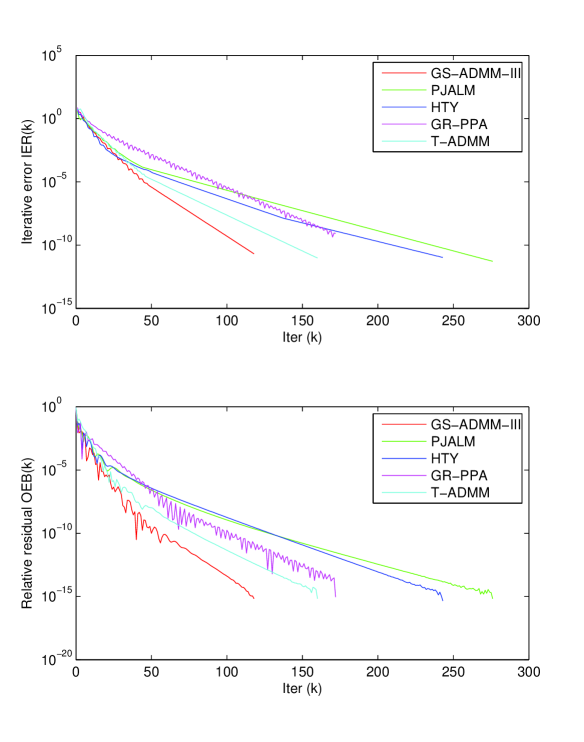
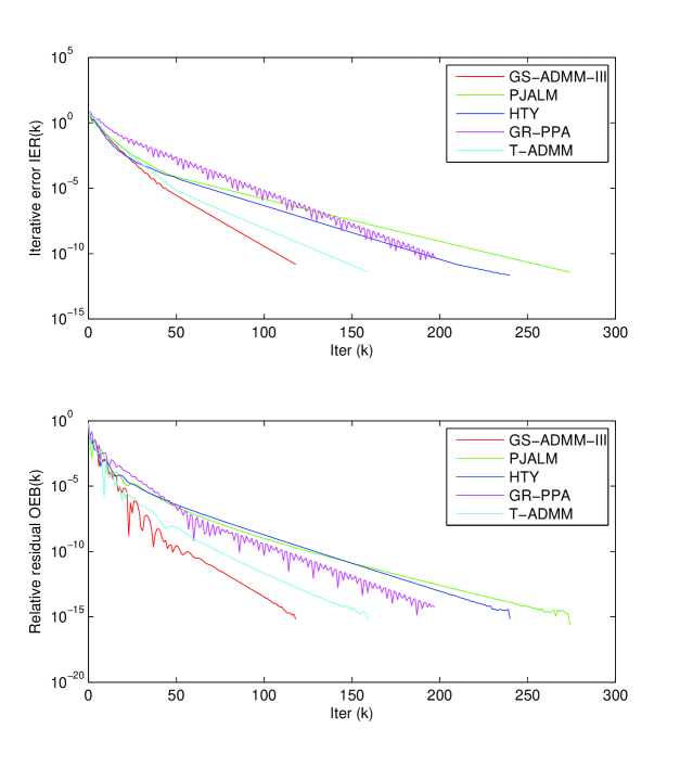
Fig. 1: Convergence curves of IER and OER with initial values $(X^{0},S^{0},L^{0},\Lambda^{0})=(\textbf{I},2\textbf{I},\textbf{I},\textbf{0})$.

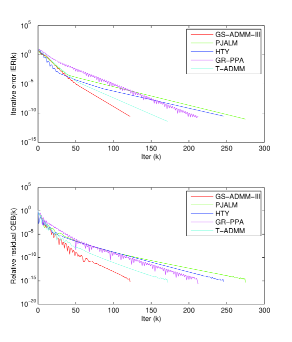
Fig. 2: Convergence curves of IER and OER with initial values $(X^{0},S^{0},L^{0},\Lambda^{0})=(\textbf{I},\textbf{I},\textbf{0},\textbf{0})$.

Fig. 3: Convergence curves of IER and OER with initial values $(X^{0},S^{0},L^{0},\Lambda^{0})=(\textbf{I},4\textbf{I},3\textbf{I},\textbf{0})$.

Acknowledgements. The authors would like to thank the anonymous referees for providing very constructive comments. The first author also wish to thank Prof. Defeng Sun at National University of Singapore for his valuable discussions on ADMM and Prof. Pingfan Dai at Xi’an Jiaotong University for discussion on an early version of the paper.

References

- (1) Bai, J.C., Li, J.C., Li, J.F.: A novel parameterized proximal point algorithm with applications in statistical learning. Optimization Online, March, (2017) http://www.optimization-online.org/DB_HTML/2017/03/5901.html.
- (2) Chandrasekaran, V., Parrilo, P.A., Willsky, A.S.: Latent variable graphical model selection via convex optimization. Ann. Stat. 40, 1935-1967 (2012)
- (3) Chen, C.H., He, B.S., Ye, Y.Y., Yuan, X.M.: The direct extension of ADMM for multi-block minimization problems is not necessarily convergent. Math. Program. 155, 57-79 (2016)
- (4) Dong, B., Yu, Y., Tian, D.D.: Alternating projection method for sparse model updating problems. J. Eng. Math. 93, 159-173 (2015)
- (5) Fortin, M., Glowinski, R.: Augmented Lagrangian Methods: Applications to the Numerical Solution of Boundary-Value Problems. P.299-331. North-Holland, Amsterdam (1983)
- (6) Facchinei, F., Pang, J.S.: Finite-Dimensional Variational Inequalities and Complementarity Problems. Springer Ser. Oper. Res. 1, Springer, New York (2003)
- (7) Fortin, M.: Numerical methods for Nonlinear Variational Problems. Springer-Verlag, New York (1984)
- (8) Glowinski, R. Marrocco, A.: Approximation parlments finis d’rdre un et rsolution, par pnalisation-dualit d’une classe de problmes de Dirichlet non linaires. Rev. Fr. Autom. Inform. Rech. Opr. Anal. Numr. 2, 41-76 (1975)
- (9) Gu, Y., Jiang, B., Han, D.: A semi-proximal-based strictly contractive Peaceman-Rachford splitting method. arXiv:1506.02221, (2015)
- (10) Hestenes, M.R.: Multiplier and gradient methods. J. Optim. Theory Appl. 4, 303-320 (1969)
- (11) He, B.S., Yuan, X.M.: On the convergence rate of the Douglas-Rachford alternating direction method. SIAM J. Num. Anal. 50, 700-709 (2012)
- (12) He, B.S., Liu, H., Wang, Z.R., Yuan, X.M.: A strictly contractive Peaceman-Rachford splitting method for convex programming. SIAM J. Optim. 24, 1011-1040 (2014)
- (13) He, B.S., Hou, L.S., Yuan, X.M.: On full Jacobian decomposition of the augmented Lagrangian method for separable convex programming. SIAM J. Optim. 25, 2274-2312 (2015)
- (14) He, B.S., Tao, M., Yuan, X.M.: A splitting method for separable convex programming. IMA J. Numer. Anal. 31, 394-426 (2015)
- (15) He, B.S., Yuan, X.M.: Block-wise alternating direction method of multipliers for multiple-block convex programming and beyond. SMAI J. Comput. Math. 1, 145-174 (2015)
- (16) He, B.S., Ma, F., Yuan, X.M.: Convergence study on the symmetric version of ADMM with larger step sizes. SIAM J. Imaging Sci. 9, 1467-1501 (2016)
- (17) He, B.S., Xu, H.K., Yuan, X.M.: On the proximal Jacobian decomposition of ALM for multiple-block separable convex minimization problems and its relationship to ADMM. J. Sci. Comput. 66, 1204-1217 (2016)
- (18) He, B.S.: On the convergence properties of alternating direction method of multipliers. Numer. Math.: A Journal of Chinese Universities(Chinese Series) 39, 81-96 (2017).
- (19) Liu, Z.S., Li, J.C., Li, G., Bai, J.C., Liu, X.N.: A new model for sparse and low-rank matrix decomposition. J. Appl. Anal. Comput. 7, 600-616 (2017)
- (20) Ma, S.Q.: Alternating proximal gradient method for convex minimization. J. Sci. Comput. 68, 546-572 (2016)
- (21) Rothman, A.J., Bickel, P.J., Levina, E., Zhu, J.: Sparse permutation invariant covariance estimation. Electron. J. Stat. 2, 494-515 (2008)
- (22) Tao, M., Yuan, X.M.: Recovering low-rank and sparse components of matrices from incomplete and noisy observations. SIAM J. Optim. 21, 57-81 (2011)
- (23) Wang, J.J., Song, W.: An algorithm twisted from generalized ADMM for multi-block separable convex minimization models. J. Comput. Appl. Math. 309, 342-358 (2017)