A Sequential Quadratic Programming Method for Constrained Multi-objective Optimization Problems

Abstract

In this article, a globally convergent sequential quadratic programming (SQP) method is developed for multi-objective optimization problems with inequality type constraints. A feasible descent direction is obtained using a linear approximation of all objective functions as well as constraint functions. The sub-problem at every iteration of the sequence has feasible solution. A non-differentiable penalty function is used to deal with constraint violations. A descent sequence is generated which converges to a critical point under the Mangasarian-Fromovitz constraint qualification along with some other mild assumptions. The method is compared with a selection of existing methods on a suitable set of test problems.

1 Introduction

A widely used line search technique for solving constrained single objective optimization problems is SQP method, which was developed by Wilson in 1963 and modified by several researchers (see mang1 ; rob1 ) in various directions. A serious limitation of these methods is the inconsistency of the quadratic sub-problem. Powell (powell ) suggested a modified sub-problem to overcome this restriction, which was further modified in burke1 ; liu2 ; mo1 for better efficiency. SQP method in burke1 converges to an infeasible point in some situations. SQP method in liu1 is a two step method. But, SQP method in mo1 is one step method and always converges to a feasible point. These developments are related to single objective optimization problems. In this article, a convergent SQP iterative scheme is developed for constrained multi-objective optimization problems, in the light of mo1 .

Classical methods for solving multi-objective optimization problems are either scalarization methods or heuristic methods. Scalarization methods reduce the multi-objective optimization problem to a single objective optimization problem using pre determined parameters. Heuristic methods do not guarantee the convergence to the solution. To address these limitations, line search methods for unconstrained multi-objective optimization problems have been developed since 2000 by many researchers (mat1 ; mat2 ; flg1 ; flg2 ; pav1 ), which are treated as the extension of single objective line search techniques. Possible extension of these concepts to constrained multi-objective problems is an interesting area of research in recent times.

The steepest descent method for multi-objective problems developed by Fliege and Svaiter (flg2 ) uses the linear approximation of all objective functions to find a descent direction. This concept is extended in drummond1 to projected gradient method for vector optimization problems, which is further extended in fukuda1 ; cruz1 in different directions. An interior point algorithm is developed in miglierina1 for box constrained multi-objective optimization problems using the concept of vector pseudo gradient. Recently Fliege and Vaz (flg3 ) and Gebken et al. (Bennet1 ) have developed SQP methods for constrained multi-objective optimization problems using the ideas of single objective SQP methods. The sub-problem in flg3 is not necessarily feasible at every iteration step. Some restoration process is used to make the sub-problem feasible, and approximate Pareto front is generated. The SQP method in Bennet1 requires feasible initial approximation, which is very difficult in nonlinear constrained problems. In addition to this, the iterative process in Bennet1 does not use penalty function, and only active constraints are used in the sub-problem. In this article these difficulties are taken care. A modified SQP scheme is developed using a different sub-problem so that the infeasibility of the sub-problem at every iteration step can be avoided and a non-differentiable penalty function is used to restrict constraint violations.

The outline of this article is as follows. Some preliminaries on the existence of the solution of a multi-objective optimization problem are discussed in Section 2. A modified SQP scheme for inequality constrained multi-objective optimization problems is developed in Section 3 and global convergence of this scheme is proved in Section 4. In Section 5, the proposed method is compared with existing methods using a set of test problems.

2 Preliminaries

Consider the multi-objective optimization problem:

$$MOP:\leavevmode\nobreak\ \leavevmode\nobreak\ \leavevmode\nobreak\ \min\leavevmode\nobreak\ \leavevmode\nobreak\ \left(f_{1}(x),f_{2}(x),...,f_{m}(x)\right)$$

$$\leavevmode\nobreak\ \leavevmode\nobreak\ \mbox{s.t. }g_{i}(x)\leq 0,\leavevmode\nobreak\ \leavevmode\nobreak\ \leavevmode\nobreak\ i=1,2,...,p,$$

where $f_{j},g_{i}:\mathbb{R}^{n}\rightarrow\mathbb{R}$ are continuously differentiable for $j\in\{1,2,...,m\}$ and $i\in\{1,2,...,p\}$. Denote $\mathbb{R}^{n}_{+}=\{x\in\mathbb{R}^{n}|x_{i}\geq 0,i=1,2,...,n\}$,
$\Lambda_{n}=\{1,2,...,n\}$ for any $n\in\mathbb{N}$, and the feasible set of the $MOP$ as
$X=\{x\in\mathbb{R}^{n}:g_{i}(x)\leq 0,\leavevmode\nobreak\ i\in\Lambda_{p}\}$. Inequality in $\mathbb{R}^{n}$ is understood componentwise. If there exists $x\in X$ which minimizes all objective functions simultaneously then it is an ideal solution. But in practice, decrease of one objective function may cause increase of another objective function. So, in the theory of multi-objective optimization, optimality is replaced by efficiency. A feasible point $x^{*}\in X$ is said to be an efficient solution of the $MOP$ if there does not exist $x\in X$ such that $f(x)\leq f(x^{*})$ and $f(x)\neq f(x^{*})$ hold where $f(x)=(f_{1}(x),f_{2}(x),...,f_{m}(x))$. A feasible point $x^{*}\in X$ is said to be a weak efficient solution of $MOP$ if there does not exist $x\in X$ such that $f(x)<f(x^{*})$ holds. For $x,y\in X$, we say $y$ dominates $x$, if and only if $f(y)\leq f(x)$, $f(y)\neq f(x)$. A point $x\in X$ is said to be non dominated if there does not exist any $y\in X$ such that $y$ dominates $x$. If $X^{*}$ is the set of all efficient solutions of the $MOP$, then the image of $X^{*}$ under $f$, i.e. $f(X^{*})$ is said to be the Pareto front of the $MOP.$

In our analysis, we use the $L_{\infty}$ non-differentiable penalty function

$$\Phi(x)=\max\{0,g_{i}(x),i\in\Lambda_{p}\}.$$

In order to obtain a feasible descent direction, the penalty function for the $MOP$ is used as the following merit function $\Psi_{j,\sigma}(x)$, with a penalty parameter $\sigma>0$ as

$$\Psi_{j,\sigma}(x)=f_{j}(x)+\sigma\Phi(x),\leavevmode\nobreak\ \leavevmode\nobreak\ j\in\Lambda_{m}.$$

Let $I(x)=\{i\in\Lambda_{p}:g_{i}(x)=\Phi(x)\}$ be the set of active or most violated constraints. The directional derivative of $\Phi(x)$ in any direction $d\in\mathbb{R}^{n}$ is

$$\Phi^{\prime}(x;d)=\underset{i\in I(x)}{\max}\{\nabla g_{i}(x)^{T}d\},$$

In general $\Phi^{\prime}(x;d)$ is not continuous. A continuous approximation of $\Phi^{\prime}(x;d)$ (see baz1 ) is

$$\Phi^{*}(x;d)=\underset{i\in I(x)}{\max}\{g_{i}(x)+\nabla g_{i}(x)^{T}d,0\}-\Phi(x).$$

Thus, an approximation of the directional derivative of $\Psi_{j,\sigma}(x)$ is

$$\theta_{j,\sigma}(x;d)=\nabla f_{j}(x)^{T}d+\sigma\Phi^{*}(x;d),\leavevmode\nobreak\ \leavevmode\nobreak\ j\in\Lambda_{m}.$$

If all $f_{j},g_{i}$ are continuously differentiable then the necessary condition of weak efficiency can be derived using Motzkin’s theorem as follows.

Theorem 1

(Fritz John necessary condition [Theorem 3.1.1,kmm1 ])
Suppose $f_{j}$, $j\in\Lambda_{m}$ and $g_{i}$, $i\in\Lambda_{p}$ are continuously differentiable at $x^{*}\in X$. If $x^{*}$ is a weak efficient solution of the $MOP$ then there exists $(\lambda,\mu)\in\mathbb{R}_{+}^{m}\times\mathbb{R}_{+}^{p}$, $(\lambda,\mu)\neq 0^{m+p}$ satisfying

$$\underset{j\in\Lambda_{m}}{\Sigma}\lambda_{j}\nabla f_{j}(x^{*})+\underset{i\in\Lambda_{p}}{\Sigma}\mu_{i}\nabla g_{i}(x^{*}) = 0$$ (1)

$$\mu_{i}g_{i}(x^{*}) = 0\leavevmode\nobreak\ \leavevmode\nobreak\ \forall\leavevmode\nobreak\ \leavevmode\nobreak\ i\in\Lambda_{p}.$$ (2)

The set of the vector $(\lambda,\mu)\in\mathbb{R}^{m}_{+}\times\mathbb{R}^{p}_{+}\setminus\{0^{m+p}\}$ satisfying (1) and (2) are called Fritz John multipliers associated with $x^{*}$. But the Fritz John necessary condition does not guarantee $\lambda_{j}>0$, for at least one $j$. So some constraint qualifications or regularity conditions should hold to ensure it.
Several constraint qualifications or regularity conditions are defined and discussed in mae1 ; maciel1 . Through the discussion of this article we consider the Mangasarian-Fromovitz constraint qualification.

Definition 1

mfcq1 The Mangasarian-Fromovitz constraint qualification (MFCQ) is said to be satisfied at a point $x\in\mathbb{R}^{n}$, if there is a $z\in\mathbb{R}^{n}$ such that $\nabla g_{i}(x)^{T}z<0$ for $i\in I(x)$.

Suppose MFCQ holds at $x$. Then the system of inequalities $\nabla g_{i}(x)^{T}z<0$ for $i\in I(x)$ has a nonzero solution $z\in\mathbb{R}^{n}$. Hence by Gordan’s theorem of alternative $\underset{i\in I(x)}{\Sigma}\mu_{i}\nabla g_{i}(x)=0$, $\mu_{i}\geq 0$ has no nonzero solution. That is, $\mu_{i}=0$ $\forall$ $i\in I(x)$.
Conversely suppose the system $\underset{i\in I(x)}{\Sigma}\mu_{i}\nabla g_{i}(x)=0,$ $\mu_{i}\geq 0$ at $x$ has no nonzero solution $\mu$. Then by Gordan’s theorem of alternative the system of inequalities $\nabla g_{i}(x)^{T}z<0$ for $i\in I(x)$ has some nonzero solution $z\in\mathbb{R}^{n}$.

Above discussion concludes that MFCQ holds at $x$ iff

$$\underset{i\in I(x)}{\Sigma}\mu_{i}\nabla g_{i}(x)=0,\leavevmode\nobreak\ \leavevmode\nobreak\ \mu_{i}\geq 0\leavevmode\nobreak\ \leavevmode\nobreak\ \Rightarrow\leavevmode\nobreak\ \leavevmode\nobreak\ \mu_{i}=0\leavevmode\nobreak\ \leavevmode\nobreak\ \forall\leavevmode\nobreak\ \leavevmode\nobreak\ i\in I(x).$$

Strong and weak stationary points for single-objective optimization problems are defined in Definition 1 of mo1 . In the light of this definition, strong and weakly critical point of the $MOP$ can be defined, taking care all objective functions together as follows.

Definition 2

A feasible point $x$ of the $MOP$ is said to be

1. a strongly critical point of the $MOP$ if there exist vectors $\lambda\in\mathds{R}^{m}_{+}-\{0^{m}\}$ and $\mu\in\mathds{R}^{p}_{+}$ satisfying (1) and (2).

2. a weakly critical point of the $MOP$ if there exists an infeasible sequence $\{x^{k}\}$ converging to $x\in X$ such that

   $$\underset{k\rightarrow\infty}{\lim}\frac{\underset{d\in D(x^{k})}{\max}\leavevmode\nobreak\ \underset{i\in\Lambda_{p}}{\max}\{g_{i}(x^{k})+\nabla g_{i}(x^{k})^{T}d;0\}}{\Phi(x^{k})}=1,$$

   where $D(x^{k})=\{d:\nabla f_{j}(x^{k})^{T}d\leq 0,\leavevmode\nobreak\ j\in\Lambda_{m}\}.$

One may observe that a strongly critical point is a KKT point of the $MOP$.

3 A SQP based line search method for MOP

In order to obtain a feasible descent direction at $x$, we solve a quadratic programming sub-problem $QP(x)$ at $x$ as

$$QP(x):\leavevmode\nobreak\ \leavevmode\nobreak\ \underset{t,d}{\min}\leavevmode\nobreak\ \leavevmode\nobreak\ t+\frac{1}{2}d^{T}d\leavevmode\nobreak\ \leavevmode\nobreak\$$

$$\mbox{s. t. }\nabla f_{j}(x)^{T}d \leq t\leavevmode\nobreak\ \leavevmode\nobreak\ \leavevmode\nobreak\ \leavevmode\nobreak\ j\in\Lambda_{m}$$ (3)

$$g_{i}(x)+\nabla g_{i}(x)^{T}d \leq t\leavevmode\nobreak\ \leavevmode\nobreak\ \leavevmode\nobreak\ \leavevmode\nobreak\ i\in\Lambda_{p}.$$ (4)

Motivation for this sub-problem comes from flg2 with modifications to address infeasibility. Notice that $t=\Phi(x)$, $d=0$ is a feasible solution of $QP(x)$. Hence the feasibility of the sub-problem is guaranteed. $QP(x)$ has unique solution since this is a convex quadratic problem. The solutions of $QP(x)$ satisfy MFCQ since the system

$$-\underset{j\in\Lambda_{m}}{\Sigma}\gamma_{j}-\underset{i\in\Lambda_{p}}{\Sigma}\eta_{i} = 0$$

$$\underset{j\in\Lambda_{m}}{\Sigma}\gamma_{j}\nabla f_{j}(x)+\underset{i\in\Lambda_{p}}{\Sigma}\eta_{i}\nabla g_{i}(x) = 0$$

$$\gamma_{j}\geq 0,\eta_{i}\geq 0$$

implies $\gamma_{j}=0$ for all $j$ and $\eta_{i}=0$ for all $i$. Hence there exist $\lambda\in\mathbb{R}^{m}_{+}$, $\mu\in\mathbb{R}^{p}_{+}$, $(\lambda,\mu)\neq 0^{m+p}$ satisfying the KKT optimality conditions. As a result,

$$d+\underset{j\in\Lambda_{m}}{\Sigma}\lambda_{j}\nabla f_{j}(x)+\underset{i\in\Lambda_{p}}{\Sigma}\mu_{i}\nabla g_{i}(x)=0,$$ (5)

$$1-\underset{j\in\Lambda_{m}}{\Sigma}\lambda_{j}-\underset{i\in\Lambda_{p}}{\Sigma}\mu_{i}=0,$$ (6)

$$\lambda_{j}\geq 0,\leavevmode\nobreak\ \leavevmode\nobreak\ \leavevmode\nobreak\ \leavevmode\nobreak\ \lambda_{j}(\nabla f_{j}(x)^{T}d-t)=0,\leavevmode\nobreak\ \leavevmode\nobreak\ \leavevmode\nobreak\ j\in\Lambda_{m},$$ (7)

$$\mu_{i}\geq 0,\leavevmode\nobreak\ \leavevmode\nobreak\ \leavevmode\nobreak\ \leavevmode\nobreak\ \mu_{i}(g_{i}(x)+\nabla g_{i}(x)^{T}d-t)=0\leavevmode\nobreak\ \leavevmode\nobreak\ \leavevmode\nobreak\ i\in\Lambda_{p},$$ (8)

$$\nabla f_{j}(x)^{T}d-t\leq 0,\leavevmode\nobreak\ \leavevmode\nobreak\ j\in\Lambda_{m},$$ (9)

$$\leavevmode\nobreak\ \leavevmode\nobreak\ g_{i}(x)+\nabla g_{i}(x)^{T}d-t\leq 0\leavevmode\nobreak\ \leavevmode\nobreak\ i\in\Lambda_{p}.$$ (10)

Lemma 1

Suppose that $(t,d)$ is the solution of the $QP(x)$.

1. Then

   $$t\leq\Phi(x)-\frac{1}{2}d^{T}d.$$ (11)

2. If $d=0$ and the MFCQ holds at $x$ then $x$ is a strong critical point of MOP.

3. If $d\neq 0$ then $d$ is a descent direction of $\Psi_{j,\sigma}(x)$ at $x$ for $\sigma$ sufficiently large.

Proof:
(I) One can observe that $t=\Phi(x)$, $d=0$ is a feasible solution of $QP(x)$. Hence $t+\frac{1}{2}d^{T}d\leq\Phi(x)$. This implies

$$t\leq\Phi(x)-\frac{1}{2}d^{T}d.$$

(II) Suppose $(t,0)$ is the solution of $QP(x)$. Replacing $d$ by $0$ in (5)-(10), we get

$$\underset{j\in\Lambda_{m}}{\Sigma}\lambda_{j}\nabla f_{j}(x)+\underset{i\in\Lambda_{p}}{\Sigma}\mu_{i}\nabla g_{i}(x)=0$$ (12)

$$1-\underset{j\in\Lambda_{m}}{\Sigma}\lambda_{j}-\underset{i\in\Lambda_{p}}{\Sigma}\mu_{i}=0$$ (13)

$$\lambda_{j}\geq 0\leavevmode\nobreak\ \leavevmode\nobreak\ \leavevmode\nobreak\ \leavevmode\nobreak\ \lambda_{j}t=0,\leavevmode\nobreak\ \leavevmode\nobreak\ \leavevmode\nobreak\ j\in\Lambda_{m}$$ (14)

$$\mu_{i}\geq 0\leavevmode\nobreak\ \leavevmode\nobreak\ \leavevmode\nobreak\ \mu_{i}(g_{i}(x)-t)=0\leavevmode\nobreak\ \leavevmode\nobreak\ \leavevmode\nobreak\ \leavevmode\nobreak\ i\in\Lambda_{p}$$ (15)

$$0\leq t,\leavevmode\nobreak\ \leavevmode\nobreak\ \leavevmode\nobreak\ \leavevmode\nobreak\ g_{i}(x)\leq t\leavevmode\nobreak\ \leavevmode\nobreak\ \leavevmode\nobreak\ \leavevmode\nobreak\ i\in\Lambda_{p}.$$ (16)

$\Phi(x)\leq t$ follows from definition of $\Phi(x)$ and (16). Then $t$, satisfying (11) with $d=0$ implies $\Phi(x)\geq t$. Hence $\Phi(x)=t$. From (15), $\mu_{i}=0$ follows for all $i\notin I(x).$ Also, $\lambda_{j}>0$ holds for at least one $j$. Otherwise, (12) and (13) will imply $\underset{i\in\Lambda_{p}}{\Sigma}\mu_{i}\nabla g_{i}(x)=0$, $\mu_{i}>0$ for at least one $i$, which violates the MFCQ. This implies that $t=0=\Phi(x)$ (from (14)). That is, $x$ is a feasible point. Then from (15), $\mu_{i}g_{i}(x)=0$, $\mu_{i}\geq 0$, $i\in\Lambda_{p}.$ Therefore, $x$ is a strongly critical point of $P$, which follows from (12).
(III) Suppose $(t,d)$ is the solution of $QP(x)$ and $d\neq 0$. Then the following two cases could arise:
Case-1: Let $\Phi(x)>0$. Applying (11) in (4) we get

$$g_{i}(x)+\nabla g_{i}(x)^{T}d\leq t\leq\Phi(x)-\frac{1}{2}d^{T}d < \Phi(x).$$

Since $0<\Phi(x)$, we have $\underset{i\in I(x)}{\max}\{g_{i}(x)+\nabla g_{i}(x)^{T}d,0\}-\Phi(x)<0$, from the inequalities above. That is, $\Phi^{*}(x;d)<0$. If $\sigma$ is chosen in such way that

$$\nabla f_{j}(x)^{T}d+\sigma\Phi^{*}(x;d)\leq-\frac{1}{2}{d}^{T}d<0$$

holds for all $j$ then $d$ will be a descent direction of $\Psi_{j,\sigma}(x)$ for all $j$ (from Lemma 2.1(1) of baz1 ).
Case-2: If $\Phi(x)=0$, then $t=0$, $d=0$ is a feasible solution of $QP(x)$. So $g_{i}(x)+\nabla g_{i}(x)^{T}d\leq t\leq 0$ holds for all $i\in I(x)$. So

$$\Phi^{*}(x;d)=\underset{i\in I(x)}{\max}\{g_{i}(x)+\nabla g_{i}(x)^{T}d,0\}-\Phi(x)=0.$$

Also, $d\neq 0$ implies $t<0$. Hence from (3), we have $\nabla f_{j}(x)^{T}d\leq t<0$ and consequently $\nabla f_{j}(x)^{T}d+\sigma\Phi^{*}(x;d)<0$.∎Let $(t^{k},d^{k})$ be the solution of the subproblem $QP(x^{k})$. Following the arguments of the proof of Lemma 1(III), the penalty parameter $\sigma_{k}$ can be updated to force $d^{k}$ to remain a descent direction for all $\Psi_{j,\sigma_{k+1}}(x^{k}).$ At $k^{th}$ iteration $\sigma_{k}$ is unchanged if $d^{k}$ is the descent direction. Otherwise, $\sigma_{k}$ is updated as

$$\sigma_{k+1}=\max\left\{2\sigma_{k},\frac{\nabla f_{j}(x^{k})^{T}d^{k}+\frac{1}{2}{d^{k}}^{T}d^{k}}{-\Phi^{*}(x^{k};d^{k})},\leavevmode\nobreak\ j\in\Lambda_{m}\right\}.$$ (17)

The theoretical results developed so far are summarized in the following algorithm.

Algorithm 1

(A SQP based algorithm)

1. (Initialization) Choose $x^{0}\in\mathbb{R}^{n}$, some scalars $r\in(0,1)$, $\beta\in(0,1)$, the initial penalty parameter $\sigma_{0}>0$, and an error tolerance $\epsilon$. Set $k:=0$.

2. Solve the $QP(x^{k})$ to find the descent direction $(t^{k};d^{k})$ with Lagrange multipliers $(\lambda^{k}$, $\mu^{k})$. If $\|d^{k}\|<\epsilon$, then stop, otherwise go to Step 3.

3. If $\Phi(x^{k})=0$ or $\theta_{j,\sigma_{k}}(x^{k};d^{k})\leq-\frac{1}{2}{d^{k}}^{T}d^{k}$ for all $j$, let $\sigma_{k+1}=\sigma_{k}$. Otherwise, $\sigma_{k+1}$ is updated using (17).

4. Compute step length $\alpha_{k}$ as the first number in the sequence $\{1,r,r^{2},...\}$ satisfying

   $$\Psi_{j,\sigma_{k+1}}(x^{k}+\alpha_{k}d^{k})-\Psi_{j,\sigma_{k+1}}(x^{k})\leq\alpha_{k}\beta\theta_{j,\sigma_{k+1}}(x^{k};d^{k})\leavevmode\nobreak\ \leavevmode\nobreak\ \leavevmode\nobreak\ \leavevmode\nobreak\ \forall\leavevmode\nobreak\ \leavevmode\nobreak\ j\in\Lambda_{m}.$$

   (18)

5. Update $x^{k+1}=x^{k}+\alpha_{k}d^{k}$. Set $k:=k+1$ and go to Step 2.

4 Convergence

In this section the global convergence of Algorithm 1 is proved. The following lemma is used to establish that Step 4 is well-defined. The extension to the multi-objective case justifies the convergence analysis.

Lemma 2

Suppose $\nabla f_{j}(x)$ and $\nabla g_{i}(x)$ are Lipschitz continuous for every $j\in\Lambda_{m}$ and $i\in\Lambda_{p}$ with Lipschitz constant $L$ and let $(t^{k},d^{k})$ be the solution of the $QP(x^{k})$ with $d^{k}\neq 0$. Then (18) holds for $\alpha$ sufficiently small.

Proof: Since $\nabla f_{j}(x)$ and $\nabla g_{i}(x)$ are Lipschitz continuous for every $j\in\Lambda_{m}$ and $i\in\Lambda_{p}$, from Lemma 2.1(3) of baz1 , there exists $L>0$ such that

$$\Psi_{j,\sigma_{k+1}}(x^{k}+\alpha d^{k})\leq\Psi_{j,\sigma_{k+1}}(x^{k})+\alpha\theta_{j,\sigma_{k+1}}(x^{k};d^{k})+\frac{1}{2}(1+\sigma_{k+1})L\alpha^{2}\|d^{k}\|^{2}$$

holds for every $\alpha\in[0,1]$. Hence for every $\alpha\in[0,1]$ and $\beta\in(0,1)$ (initialized in Step 1 of Algorithm 1) we have,

$$\Psi_{j,\sigma_{k+1}}(x^{k}+\alpha d^{k})-\Psi_{j,\sigma_{k+1}}(x^{k})-\beta\alpha\theta_{j,\sigma_{k+1}}(x^{k};d^{k})$$

$$\leq(1-\beta)\alpha\theta_{j,\sigma_{k+1}}(x^{k};d^{k})+\frac{1}{2}(1+\sigma_{k+1})L\alpha^{2}\|d^{k}\|^{2}.$$ (19)

Since $d^{k}\neq 0$, from Step 3 of Algorithm 1,

$$(1-\beta)\theta_{j,\sigma_{k+1}}(x^{k};d^{k})\leq-\frac{1}{2}(1-\beta)\|d^{k}\|^{2}<0.$$

Hence from (19), (18) holds for every $\alpha>0$ sufficiently small.∎

Lemma 3

Let $(t^{k},d^{k})$ be the solution of the sub-problem $QP(x^{k})$ and assume that the sequences $\{x^{k}\}$ and $\{(t^{k},d^{k})\}$ are bounded. If $x^{k}\rightarrow x^{*}$ as $k\rightarrow\infty$, then $\{(t^{k},d^{k})\}$ converges to $(t^{*},d^{*})$, where $(t^{*},d^{*})$ is the solution of $QP(x^{*})$.
In particular, if $d^{k}$ converges to $0$ and the MFCQ holds at every $x^{k}$ then $x^{*}$ is a strongly critical point of the $MOP$.

Proof: If possible let $\{x^{k}\}$ converges to $x^{*}$ but $\{(t^{k},d^{k})\}$ does not converge to $(t^{*},d^{*})$. Since $\{(t^{k},d^{k})\}$ is bounded, there exists a sub sequence $\{(t^{k},d^{k})\}_{k\in K}$ converging to $(\bar{t},\bar{d})\neq(t^{*},d^{*})$. Since $(t^{k},d^{k})$ is the optimal solution of $QP(x^{k})$, there exists $(\lambda^{k},\mu^{k})$ such that $(t^{k},d^{k};\lambda^{k},\mu^{k})$ satisfies the KKT optimality conditions (5)-(10). Now (6) implies $\{\lambda^{k}\}$ and $\{\mu^{k}\}$ are bounded. Hence there exists a converging sub sequence of the subsequence $\{(\lambda^{k},\mu^{k})\}_{k\in K}.$ Without loss of generality we may assume $\lambda^{k}\rightarrow\lambda^{*}$ and $\mu^{k}\rightarrow\mu^{*}$ as $k\rightarrow\infty$ and $k\in K$. Hence in (5)-(10), taking limit $k\rightarrow\infty$, $k\in K$, we have

$$\bar{d}+\underset{j\in\Lambda_{m}}{\Sigma}\lambda_{j}^{*}\nabla f_{j}(x^{*})+\underset{i\in\Lambda_{p}}{\Sigma}\mu_{i}^{*}\nabla g_{i}(x^{*})=0,$$

$$1-\underset{j\in\Lambda_{m}}{\Sigma}\lambda_{j}^{*}-\underset{i\in\Lambda_{p}}{\Sigma}\mu_{i}^{*}=0,$$

$$\lambda_{j}^{*}\geq 0\leavevmode\nobreak\ \leavevmode\nobreak\ \leavevmode\nobreak\ \leavevmode\nobreak\ \lambda_{j}^{*}(\nabla f_{j}(x^{*})^{T}\bar{d}-\bar{t})=0,\leavevmode\nobreak\ \leavevmode\nobreak\ \leavevmode\nobreak\ j\in\Lambda_{m},$$

$$\mu_{i}^{*}\geq 0\leavevmode\nobreak\ \leavevmode\nobreak\ \leavevmode\nobreak\ \leavevmode\nobreak\ \mu_{i}^{*}(g_{i}(x^{*})+\nabla g_{i}(x^{*})^{T}\bar{d}-\bar{t})=0\leavevmode\nobreak\ \leavevmode\nobreak\ \leavevmode\nobreak\ i\in\Lambda_{p},$$

$$\nabla f_{j}(x^{*})^{T}\bar{d}-\bar{t}\leq 0,\leavevmode\nobreak\ \leavevmode\nobreak\ j\in\Lambda_{m},$$

$$\leavevmode\nobreak\ \leavevmode\nobreak\ g_{i}(x^{*})+\nabla g_{i}(x^{*})^{T}\bar{d}-\bar{t}\leq 0\leavevmode\nobreak\ \leavevmode\nobreak\ i\in\Lambda_{p}.$$

These imply that $(\bar{t},\bar{d};\lambda^{*},\mu^{*})$ satisfies first order necessary conditions of the convex quadratic programming sub-problem $QP(x^{*})$. Hence $(\bar{t},\bar{d})$ is an optimal solution of $QP(x^{*})$. This contradicts the fact that $(t^{*},d^{*})$ is the optimal solution of $QP(x^{*})$, since $QP(x^{*})$ has unique solution. Hence $\{(t^{k},d^{k})\}$ converges to $(t^{*},d^{*})$.
In particular, if $d^{k}$ converges to $0$ and the MFCQ holds at every $x^{k}$ then replacing $d^{*}$ by $0$ in (5)-(10) at $(x^{*},t^{*},d^{*},\lambda^{*},\mu^{*})$ and proceeding as in Lemma 1(II) it is easy to prove that $x^{*}$ is a strongly critical point of the $MOP$.∎

Lemma 4

Suppose that $\sigma_{k}=\sigma>0$ for $k$ large enough, the sequences $\{x^{k}\}$ and $\{(t^{k},d^{k})\}$ are bounded, $\nabla f_{j}(x)$ and $\nabla g_{i}(x)$ are Lipschitz continuous for every $j\in\Lambda_{m}$ and $i\in\Lambda_{p}$ with Lipschitz constant $L$, and $\{x^{k}\}_{k\in K}$ is a convergent subsequence. Then $d^{k}\rightarrow 0$ as $k\rightarrow\infty$ and $k\in K$.

Proof: Without loss of generality, assume that $\sigma_{k}=\sigma$ for all $k\in K$. If possible suppose that there exists an infinite subset $K^{{}^{\prime}}\subset K$ and a positive constant $\eta$ such that

$$\|d^{k}\|\geq\eta,\leavevmode\nobreak\ \leavevmode\nobreak\ \leavevmode\nobreak\ \leavevmode\nobreak\ \leavevmode\nobreak\ k\in K^{{}^{\prime}}.$$ (20)

First we will show that there exists $\delta>0$ such that $\alpha_{k}\geq\delta$ holds for every $k$, where $\alpha_{k}$ is the step length obtained in Step 4 of Algorithm 1. From this step either $\alpha_{k}=1$ or $\alpha_{k}=r^{k_{1}}$ holds for some $k_{1}\in\mathbb{N}$. If $\alpha_{k}=r^{k_{1}}$ holds then there exists $\hat{j}\in\Lambda_{m}$ satisfying,

$$\Psi_{\hat{j},\sigma}(x^{k}+r^{k_{1}-1}d^{k})-\Psi_{\hat{j},\sigma}(x^{k})>r^{k_{1}-1}\beta\theta_{\hat{j},\sigma}(x^{k};d^{k}).$$

Then from (19),

$$\frac{1}{2}(1+\sigma)Lr^{2(k_{1}-1)}\|d^{k}\|^{2}\geq-r^{k_{1}-1}(1-\beta)\theta_{\hat{j},\sigma}(x^{k};d^{k}).$$

From Step 3 of Algorithm 1,

$$\frac{1}{2}(1+\sigma)Lr^{k_{1}-1}\|d^{k}\|^{2} \geq \frac{1}{2}(1-\beta)\|d^{k}\|^{2}$$

$$\Rightarrow r^{k_{1}} \geq \frac{r(1-\beta)}{(1+\sigma)L}$$

Choose $\delta=\min\{1,\frac{r(1-\beta)}{(1+\sigma)L}\}$. Then $\alpha_{k}\geq\delta$ holds for every $k$. Now

$$\Psi_{j,\sigma}(x^{k+1})-\Psi_{j,\sigma}(x^{0}) = \Sigma_{l=0}^{k}\Psi_{j,\sigma}(x^{l}+\alpha_{l}d^{l})-\Psi_{j,\sigma}(x^{l})$$

$$\leq -\frac{\beta}{2}\Sigma_{l=0}^{k}\alpha_{k}\|d^{k}\|^{2}$$

$$\leq -\frac{1}{2}(k+1)\delta\beta\eta^{2}\leavevmode\nobreak\ \leavevmode\nobreak\ \forall k\in K^{\prime}.$$

The second inequality follows from (18) and Step 3 of Algorithm 1. This implies $\Psi_{j,\sigma}(x^{k}+\alpha_{k}d^{k})\rightarrow-\infty$ as $k\rightarrow\infty$ and $k\in K^{\prime}$ (since $\alpha_{0}\beta\eta^{2}>0$). This contradicts the assumption that $\{x^{k}\}$, $\{(t^{k},d^{k})\}$ are bounded as $\Psi_{j,\sigma}$ is a continuous function. So there does not exist any $K^{{}^{\prime}}\subset K$ and $\eta>0$ such that (20) holds. Hence the lemma follows.∎

Lemma 5

If $\sigma_{k}\rightarrow\infty$ and the sequences $\{x^{k}\}$, $\{(t^{k},d^{k})\}$ are bounded then $\underset{k\rightarrow\infty}{\lim}\Phi(x^{k})=0.$

Proof: Proof of this result is similar to the proof of Lemma 7 in mo1 .∎

Theorem 2

Let $\{x^{k}\}$ be a sequence generated by Algorithm 1, the sequences $\{x^{k}\}$ and $\{(t^{k},d^{k})\}$ are bounded, $\nabla f_{j}(x)$ and $\nabla g_{i}(x)$ are Lipschitz continuous for every $j\in\Lambda_{m}$ and $i\in\Lambda_{p}$ with Lipschitz constant $L$, and the MFCQ is satisfied at every $x^{k}$. Then any accumulation point of $\{x^{k}\}$ is a critical point (either weak or strongly critical point) of the $MOP$.

Proof:
$(i)$ Convergence to a strongly critical point:
Let $K$ be an infinite index set such that $x^{k}\rightarrow x^{*}$ as $k\rightarrow\infty$ and $k\in K$. Let $\{(t^{k},d^{k})\}$ be the solution of $QP(x^{k})$. If $d^{k}\rightarrow 0$ as $k\rightarrow\infty$ then by Lemma 3, $x^{*}$ is a strongly critical point of $P$.
$(ii)$ Convergence to a weakly critical point:
If there exists a constant $c_{0}>0$ such that $\|d^{k}\|\geq c_{0}$ for large $k\in K$ then from Lemma 4, $\sigma_{k}\rightarrow\infty$ as $k\rightarrow\infty$. Since the sequences $\{x^{k}\}$, $\{(t^{k},d^{k})\}$ are bounded, so from Lemma 5, $\underset{k\rightarrow\infty}{\lim}\Phi(x^{k})=0$. Hence from (11) and (3),

$$\nabla f_{j}(x^{k})^{T}d\leq t^{k}<0\leavevmode\nobreak\ \leavevmode\nobreak\ \forall\leavevmode\nobreak\ \leavevmode\nobreak\ j\in\Lambda_{m}.$$

This implies, $d^{k}\in D(x^{k})$ for large $k$. Assume ad absurdum that there exists a constant $\eta_{2}>0$ such that for sufficiently large $k$,

$$\underset{d\in D(x^{k})}{\max}\underset{i\in\Lambda_{p}}{\max}\{g_{i}(x^{k})+\nabla g_{i}(x^{k})^{T}d;0\}\leq\Phi(x^{k})-\eta_{2}.$$

Suppose $\hat{d^{k}}$ maximizes $\underset{i\in\Lambda_{p}}{\max}\{g_{i}(x^{k})+\nabla g_{i}(x^{k})^{T}\hat{d^{k}},0\}$. Then

$$\theta_{j,\sigma_{k+1}}(x^{k};d^{k})+\frac{1}{2}{d^{k}}^{T}d^{k} \leq \Phi(x^{k})+\sigma_{k}\left(\underset{i\in\Lambda_{P}}{\max}\{g_{i}(x^{k})+\nabla g_{i}(x^{k})^{T}\hat{d^{k}},0\}-\Phi(x^{k})\right)$$

$$\leq \Phi(x^{k})-\eta_{2}\sigma_{k}$$

$$< 0.$$

This contradicts Step 3 of the Algorithm. As a result, $\{x^{k}\}$ converges to a weakly critical point.
Hence any accumulation point of $\{x^{k}\}$ is either a strongly critical point or a weakly critical point.∎

5 Numerical illustration and discussion

In this section the proposed method (Algorithm 1) (MOSQP) is compared with a classical method (weighted sum method (MOS)) and the method developed by Fliege and Vaz flg3 (MOSQP(F)). In order to compare different methods we use the performance profiles presented in flg3 ; zitq ; zitp with respect to the purity metric and the $\Gamma$ and $\Delta$ spread metrics. (The readers may see the details in flg3 ). In addition to this, two line search techniques MOSQP and MOSQP(F) are compared with respect to average function evaluations.

Performance profile: Performance profiles are defined by a cumulative function $\rho(\tau)$ representing a performance ratio with respect to a given metric, for a given set of solvers. Given a set of solvers $\mathcal{SO}$ and a set of problems $\mathcal{P}$, let $\varsigma_{p,s}$ be the performance of solver $s$ on solving problem $p$. The performance ratio is then defined as $r_{p,s}=\frac{\varsigma_{p,s}}{\underset{s\in\mathcal{SO}}{\min}\varsigma_{p,s}}$. The cumulative function $\rho_{s}(\tau)$ ($s\in\mathcal{SO}$) is defined as

$$\rho_{s}(\tau)=\frac{|\{p\in\mathcal{P}:r_{p,s}\leq\tau\}|}{|P|}.$$

It has been observed that the performance profiles are sensitive to the number and types of algorithms considered in the comparison (see gould1 ). So we have compared algorithms pairwise.
Purity metric: Purity metric is used to compare the number of non-dominated solutions obtained by different algorithms. Let $F_{p,s}$ be the approximated Pareto front of problem $p$ obtained by method $s$. Then we can build an approximation to the true Pareto front $F_{p}$ by first considering $\underset{s\in\mathcal{S}}{\cup}F_{p,s}$ and removing the dominated points. The purity metric for algorithm $s$ and problem $p$ is defined by the ratio

$$\bar{t}_{p,s}=\frac{|F_{p}|}{|F_{p,s}\cap F_{p}|}.$$

Clearly $\bar{t}_{p,s}=\infty$ implies that the algorithm is unable to generate any non-dominated point in the reference Pareto front of the corresponding problem.
Spread metrics: Two types of spread metrics ($\Gamma$ and $\Delta$) are used in order to analyze if the points generated by an algorithm are well-distributed in the approximated Pareto front of a given problem. Let $x_{1},x_{2},...x_{N}$ be the set of points obtained by a solver $s$ for problem $p$ and let these points be sorted by objective function $j$, i.e., $f_{j}(x_{i})\leq f_{j}(x_{i+1})$ $(i=1,2,...,N-1)$. Suppose $x_{0}$ is the best known approximation of global minimum of $f_{j}$ and $x_{N+1}$ is the best known global maximum of $f_{j}$, computed over all approximated Pareto fronts obtained by different solvers. Define $\delta_{i,j}=f_{j}(x_{i+1})-f_{j}(x_{i})$. Then the $\Gamma$ spread metric is defined by

$$\Gamma_{p,s}=\underset{j\in\Lambda_{m}}{\max}\leavevmode\nobreak\ \leavevmode\nobreak\ \underset{i\in\{0,1,...,N\}}{\max}\delta_{i,j}.$$

Define $\bar{\delta_{j}}$ as the average of the distances $\delta_{i,j}$, $i=1,2,...,N-1.$ For an algorithm $s$ and a problem $p$ the spread metric $\Delta_{p,s}$ is

$$\Delta_{p,s}=\underset{j\in\Lambda_{m}}{\max}\left(\frac{\delta_{0,j}+\delta_{N,j}+\Sigma_{i=1}^{N-1}|\delta_{i,j}-\bar{\delta_{j}}|}{\delta_{0,j}+\delta_{N,j}+(N-1)\bar{\delta_{j}}}\right).$$

Test problems: A set of test problems, collected from different sources, are summarized in Tables 1 and 2. Bound constrained test problems are summarized in Table 1. Linear and nonlinear constrained test problems are summarized in Table 2. In Table 2, ‘linear’ is the number of linear constraints except bound constraints, and ‘nonlinear’ is the number of nonlinear constraints. In both tables $m$ is the number of objective functions and $n$ represents the number of variables.

problem	Source	$m$	$n$	problem	Source	$m$	$n$	problem	Source	$m$	$n$
BK1	hub1	2	2	Fonseca	fonseca1	2	2	MLF1	hub1	2	1
CEC09_1	zhang1	2	30	GE2	adsc1	2	40	MLF2	hub1	2	2
CEC09_2	zhang1	2	15	GE5	adsc1	2	40	MOP1	hub1	2	1
CEC09_3	zhang1	2	30	IKK1	hub1	3	3	MOP2	hub1	2	2
CEC09_7	zhang1	2	30	IM1	hub1	2	2	MOP3	hub1	2	2
CL1	cheng1	2	4	Jin1	jin01	2	2	MOP5	hub1	3	2
Deb41	deb1999multi	2	2	Jin2_a	jin01	2	2	MOP6	hub1	2	2
Deb513	deb1999multi	2	2	Jin3	jin01	2	2	MOP7	hub1	3	2
Deb521a_a	deb1999multi	2	2	Jin4_a	jin01	2	2	SK1	hub1	2	1
Deb521b	deb1999multi	2	2	KW2	adsc1	2	2	SK2	hub1	2	4
DG01	hub1	2	1	lovison1	lovi1	2	2	SP1	hub1	2	2
DTLZ1	debs1	3	7	lovison2	lovi1	2	2	SSFYY1	hub1	2	2
DTLZ1n2	debs1	2	2	lovison3	lovi1	2	2	SSFYY2	hub1	2	1
DTLZ2	debs1	3	12	lovison4	lovi1	2	2	TKLY1	hub1	2	4
DTLZ2n2	debs1	2	2	lovison5	lovi1	3	3	VFM1	hub1	3	2
DTLZ5_a	debs1	3	12	lovison6	lovi1	3	3	VU1	hub1	2	2
DTLZ5n2_a	debs1	2	2	LRS1	hub1	2	2	VU2	hub1	2	2
ex005	hwang2	2	2	MHHM1	hub1	3	1	ZDT3	zitzler1	2	30
Far1	hub1	2	2	MHHM2	hub1	3	2

Table 1: Multi-objective test problems with bound constraints

problem	Source	$m$	$n$	linear	nonlinear	problem	Source	$m$	$n$	linear	nonlinear
ABC_Comp	hwang1	2	2	2	1	GE3	adsc1	2	2	0	2
BNH	deb1999multi	2	2	0	2	GE4	adsc1	3	3	0	1
CEC09_C3	zhang1	2	10	0	1	liswetm	leyffer1	2	7	5	0
CEC09_C9	zhang1	3	10	0	1	MOQP_002	leyffer1	3	20	9	0
ex003	tappeta	2	2	0	2	OSY	deb1999multi	2	6	4	2
ex004	oliveira1	2	2	2	0	SRN	deb1999multi	2	2	1	1
GE1	adsc1	2	2	0	1	TNK	deb1999multi	2	2	0	2

Table 2: Multi-objective test problems with linear and nonlinear constraints

Implementation details: MATLAB code (2019a) is developed for all three methods. The MATLAB code of MOSQP(F) is available in public domain, which is not used here. For MOSQP(F), we have developed own code which uses only the Step 4 (third stage) of Algorithm 4.1 flg3 since the convergence analysis of Algorithm 4.1 flg3 is different from the convergence analysis of MOSQP. Multi start techniques, similar to MOSQP, is used to generate an approximated Pareto front for MOSQP(F).

• Quadratic sub-problems are solved using MATLAB function ‘quadprog’ with ‘Algorithm’,‘interior-point-convex’.

• For MOS, the test problems are converted to single objective optimization problems and solved using MATLAB function ‘fmincon’ with ’Algorithm’ ‘sqp’, Specified ‘objective gradient’ and ‘constraint gradient’, and initial approximation as $(l+u)/2$, where $l$ and $u$ are used as in flg3 .

• $\|d^{k}\|<10^{-5}$ or a maximum of $500$ iterations are considered as stopping criteria.

• It is essential to find a set of well distributed solutions of $MOP$. Spreading out an approximation to a Pareto set is a difficult problem. One simple technique may not work always in a satisfactory manner for all type of problems. Here, to generate an approximated Pareto front, we have selected the initial point with the strategies LINE and RAND and random parameters in the scalarization method. LINE is considered only for bi-objective optimization problems and RAND is considered for both bi-objective and more than two objective optimization problems.

  • Initial point selection strategy LINE is considered for bi-objective optimization problems. Here $100$ initial points are chosen in the line segment joining $l$ and $u$, i.e. $x^{0,k}=l+k\frac{u-l}{99}$, $k=0,1,2,...,99$ and for MOS we have solved problems of the form
    $\underset{x\in X}{\min}\leavevmode\nobreak\ \leavevmode\nobreak\ wf_{1}(x)+(1-w)f_{2}(x)$ for $w=k/99$, $k=0,1,2,...,99$.

  • For every test (two or three objective) problem initial points selection strategy RAND is considered. Here $100$ random initial points are selected uniformly distributed in $l$ and $u$, and for MOS we have solved
    $\underset{x\in X}{\min}\leavevmode\nobreak\ \leavevmode\nobreak\ \underset{j\in\Lambda_{m}}{\Sigma}w_{j}f_{j}(x)$ $w_{j}\geq 0$ $w\neq 0$, where $w$ is a random vector. Every test problem is executed $10$ times with random initial points and weights.

• Restoration procedure is not used for MOSQP(F) if the quadratic sub-problem is infeasible. These points are excluded. Quadratic sub-problem ($QP(x^{k})$) of Algorithm 1 always has a solution since this is a convex quadratic problem and has at least one feasible solution.

• Different run with initial point selection strategy RAND generates different set of non-dominated points. Among 10 runs the run which generates highest number of non-dominated solutions, is denoted as best run. Similarly, the run which generates lowest number of non-dominated solutions, is denoted as worst run. Performance profiles are compared for best and worst runs.

The performance profiles between MOSQP and MOSQP(F) using purity metric of best run in RAND is provided in Figure 1(a) and the performance profiles between MOSQP and MOS using purity metric of best run in RAND is provided in Figure 1(b). Figures 2(a) and 2(b) correspond to the performance profiles for the purity metric in worst run comparing MOSQP with MOSQP(F) and MOSQP with MOS, respectively. The performance profiles for the $\Gamma$ metric in best run comparing MOSQP with MOSQP(F) and MOSQP with MOS are provided in Figures 3(a) and 3(b) respectively. The performance profiles for the $\Gamma$ metric in worst run comparing MOSQP with MOSQP(F) and MOSQP with MOS are provided in Figures 4(a) and 4(b) respectively. Figures 5(a) and 5(b) correspond to the performance profiles for $\Delta$ metric in best run comparing MOSQP with MOSQP(F) and MOSQP with MOS, respectively. The performance profiles for the $\Delta$ metric in worst run comparing MOSQP with MOSQP(F) and MOSQP with MOS are provided in Figures 6(a) and 6(b) respectively.

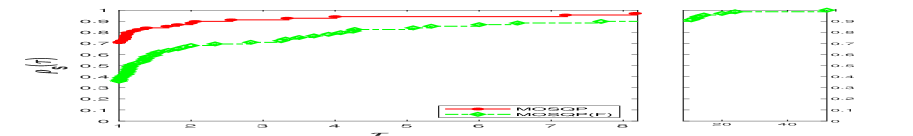
(a) Performance profile between MOSQP and MOSQP(F)

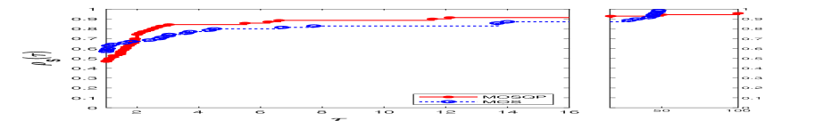
(b) Performance profile between MOSQP and MOS

Figure 1: Performance profile using purity metric in best run in RAND

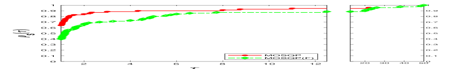
(a) Performance profile between MOSQP and MOSQP(F)

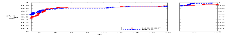
(b) Performance profile between MOSQP and MOS

Figure 2: Performance profile using purity metric in worst run in RAND

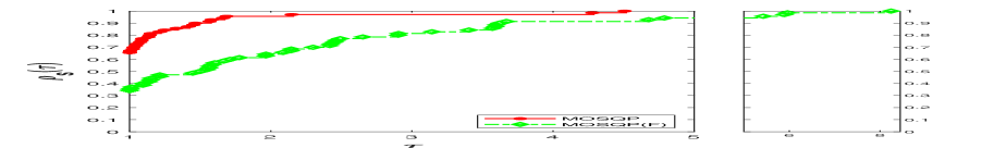
(a) Performance profile between MOSQP and MOSQP(F)

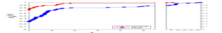
(b) Performance profile between MOSQP and MOS

Figure 3: Performance profile using $\Gamma$ metric in best run in RAND

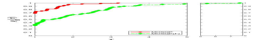
(a) Performance profile between MOSQP and MOSQP(F)

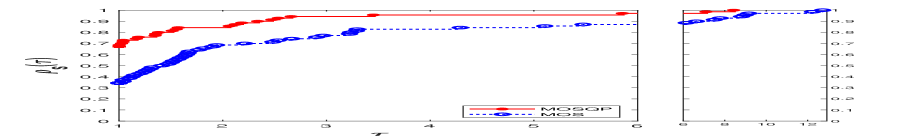
(b) Performance profile between MOSQP and MOS

Figure 4: Performance profile using $\Gamma$ metric in worst run in RAND

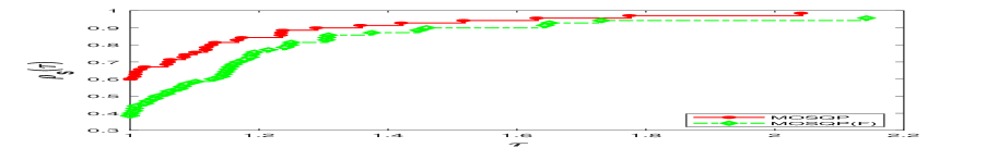
(a) Performance profile between MOSQP and MOSQP(F)

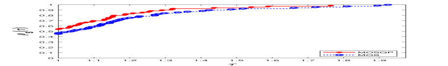
(b) Performance profile between MOSQP and MOS

Figure 5: Performance profile using $\Delta$ metric in best run in RAND

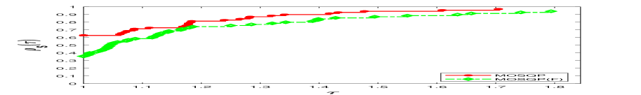
(a) Performance profile between MOSQP and MOSQP(F)

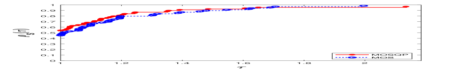
(b) Performance profile between MOSQP and MOS

Figure 6: Performance profile using $\Delta$ metric in worst run in RAND

The performance profiles using purity metric in LINE between MOSQP and MOSQP(F) and between MOSQP and MOS are provided in Figures 7(a) and 7(b) respectively. Figures 8(a) and 8(b) correspond to the performance profiles for $\Gamma$ metric in LINE comparing MOSQP with MOSQP(F) and MOSQP with MOS, respectively. The performance profiles for the $\Delta$ metric in LINE comparing MOSQP with MOSQP(F) and MOSQP with MOS are provided in Figures 9(a) and 9(b) respectively.

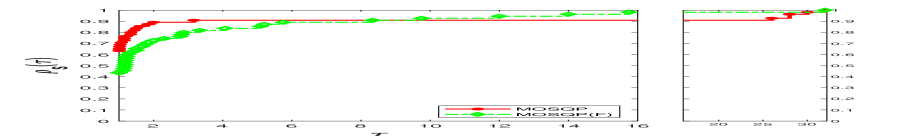
(a) Performance profile between MOSQP and MOSQP(F)

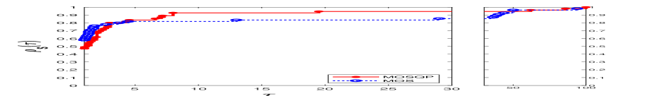
(b) Performance profile between MOSQP and MOS

Figure 7: Performance profile using purity metric in LINE

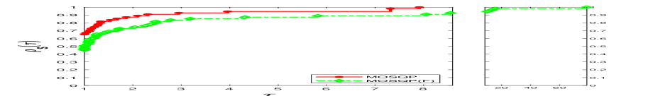
(a) Performance profile between MOSQP and MOSQP(F)

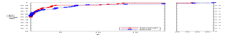
(b) Performance profile between MOSQP and MOS

Figure 8: Performance profile using $\Gamma$ metric in LINE

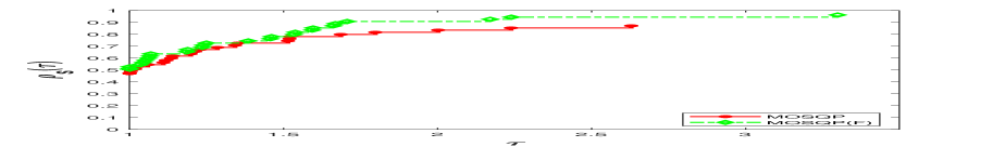
(a) Performance profile between MOSQP and MOSQP(F)

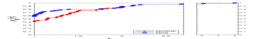
(b) Performance profile between MOSQP and MOS

Figure 9: Performance profile using $\Delta$ metric in LINE

Two line search techniques MOSQP and MOSQP(F) are compared using average number of function evaluations per non-dominated points. We have calculated gradient for MOSQP and MOSQP(F) and Hessian for MOSQP(F) using forward difference formula. If $n_{1}$ and $n_{2}$ are number of non-dominated points generated by MOSQP and MOSQP(F), then average function evaluations are derived as

$$FE_{1}=\left(\#f+n\#\nabla f\right)/n_{1}$$

and

$$FE_{2}=\left(\#f+n\#\nabla f+\frac{1}{2}n(n+1)\#\nabla^{2}f\right)/n_{2},$$

where $\#f$, $\#\nabla f$, and $\#\nabla^{2}f$ denote the number of objective function, objective gradient, and objective Hessian evaluations. Performance profiles between MOSQP and MOSQP(F) using average function evaluations in best and worst run in RAND are provided in Figures 10(a) and 10(b). Figure 11 represents performance profiles between MOSQP and MOSQP(F) using average function evaluations in LINE.

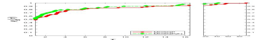
(a) Performance profile for best run

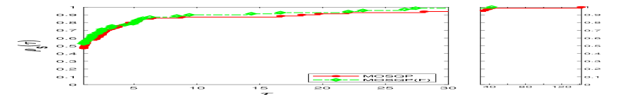
(b) Performance profile for worst run

Figure 10: Performance profile between MOSQP and MOSQP(F) using average function evaluations in RAND

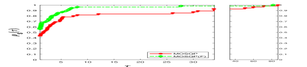
Figure 11: Performance profile between MOSQP and MOSQP(F) using average function evaluations in LINE

Result analysis: One may observe from the above figures that the method proposed in this article (MOSQP) gives better results than MOSQP(F) in purity, $\Gamma$, and $\Delta$ metrics using initial point selection strategy RAND and purity, $\Gamma$ metrics using initial point selection strategy LINE. Similarly MOSQP gives better results than MOS in $\Gamma$ metric using initial point selection strategy RAND and LINE. Other metrics have average performance ratios with MOS and MOSQP(F).

6 Conclusion

In this article we have developed a globally convergent modified SQP method for constrained multi-objective optimization problem. This method is free from any kind of a priori chosen parameters or ordering information of objective functions. Also feasibility of the sub-problem is guaranteed. To generate an approximate Pareto front, we have used the initial point selection strategies LINE and RAND. There is no single spreading technique for line search methods that can work in a satisfactory manner for all types of multi-objective programming problems. Spreading out an approximation to a Pareto front is a difficult task. A well distributed spreading technique is discussed in Step 3 of Algorithm 1.4 of flg3 . We keep the implementation of these techniques for future developments.

References

- (1) Ansary, M.A.T., Panda, G.: A modified quasi-Newton method for vector optimization problem. Optimization 64(11), 2289 2306 (2015)
- (2) Ansary, M.A.T., Panda, G.: A sequential quadratically constrained quadratic programming technique for a multi-objective optimization problem. Eng. Optim. 51(1), 22 41 (2019)
- (3) Bazaraa, M., Goode, J.: An algorithm for solving linearly constrained minimax problems. European J. Oper. Res. 11(2), 158 166 (1982)
- (4) Burke, J.V., Han, S.P.: A robust sequential quadratic programming method. Math. Program. 43(1-3), 277 303 (1989)
- (5) Cheng, F.Y., Li, X.S.: Generalized center method for multiobjective engineering optimization. Eng. Optim. 31(5), 641 661 (1999)
- (6) Cruz, J.Y.B., P erez, L.L., Melo, J.G.: Convergence of the projected gradient method for quasiconvex multiobjective optimization. Nonlinear Anal-Theor. 74(16), 5268 5273 (2011)
- (7) Deb, K.: Multi-objective genetic algorithms: Problem difficulties and construction of test problems. Evol. Comput. 7(3), 205 230 (1999)
- (8) Deb, K., Thiele, L., Laumanns, M., Zitzler, E.: Scalable multi-objective optimization test problems. In: Evolutionary Computation, 2002. CEC 02. Proceedings of the 2002 Congress on, vol. 1, pp. 825 830. IEEE (2002)
- (9) Drummond, L.M.G., Iusem, A.N.: A projected gradient method for vector optimization problems. Comput. Optim. Appl. 28(1), 5 29 (2004)
- (10) Eichfelder, G.: An adaptive scalarization method in multiobjective optimization. SIAM J. Optim. 19(4), 1694 1718 (2009)
- (11) Fliege, J., Drummond, L.M.G., Svaiter, B.F.: Newton s method for multiobjective optimization. SIAM J. Optim 20(2), 602 626 (2009)
- (12) Fliege, J., Svaiter, B.F.: Steepest descent methods for multicriteria optimization. Math. Methods Oper. Res. 51(3), 479 494 (2000)
- (13) Fliege, J., Vaz, A.I.F.: A method for constrained multiobjective optimization based on SQP techniques. SIAM J. Optim. 26(4), 2091 2119 (2016)
- (14) Fonseca, C.M., Fleming, P.J.: Multiobjective optimization and multiple constraint handling with evolutionary algorithms. I. A unified formulation. IEEE Trans. Syst. Man Cybern. A Syst. Hum. 28(1), 26 37 (1998)
- (15) Fukuda, E.H., Drummond, L. M. G.: Inexact projected gradient method for vector optimization. Comput. Optim. Appl. 54(3), 473 493 (2013)
- (16) Garcia-Palomares, U.M.G., Mangasarian, O.L.: Superlinearly convergent quasi-Newton algorithms for nonlinearly constrained optimization problems. Math. Program. 11, 1 13 (1976)
- (17) Gebken, B., Peitz, S., Dellnitz, M.: A descent method for equality and inequality constrained multiobjective optimization problems. In: L. rujillo, O. Schütze, Y. Maldonado, P. Valle (eds.) Numerical and Evolutionary Optimization-NEO 2017, pp. 29 61. Springer International Publishing, Cham (2019)
- (18) Gould, N., Scott, J.: A note on performance profiles for benchmarking software. ACM Transactions on Mathematical Software (TOMS) 43(2), 15 (2016)
- (19) Huband, S., Hingston, P., Barone, L., While, L.: A review of multiobjective test problems and a scalable test problem toolkit. IEEE Trans. Evol. Comput. 10(5), 477 506 (2006)
- (20) Hwang, C.L., Masud, A.S.M.: Multiple objective decision making methods and applications: a state-of-the-art survey. Springer Science & Business Media (1979)
- (21) Hwang, C.L., Yoon, K.: Multiple attribute decision making: methods and applications a state-of-the-art survey. Springer Science & Business Media (1981)
- (22) Jin, Y., Olhofer, M., Sendhoff, B.: Dynamic weighted aggregation for evolutionary multiobjective optimization: Why does it work and how? In: Proceedings of the Annual Conference on Genetic and Evolutionary Computation, pp. 1042 1049. Morgan Kaufmann Publishers Inc. (2001)
- (23) Leyffer, S.: A note on multiobjective optimization and complementarity constraints. Preprint ANL/MCS-P1290-0905, Mathematics and Computer Science Division, Argonne National Laboratory, Illinois, Argonne (2005)
- (24) Liu, X., Yuan, Y.: A robust algorithm for optimization with general equality and inequality constraints. SIAM J. Sci. Comput. 22(2), 517 534 (2000)
- (25) Liu, X.W.: Global convergence on an active set SQP for inequality constrained optimization. J. Comput. Appl. Math. 180(1), 201 211 (2005)
- (26) Lovison, A.: A synthetic approach to multiobjective optimization. arXiv preprint arXiv:1002.0093 (2010)
- (27) Maciel, M.C., Santos, S.A., Sottosanto, G.N.: Regularity conditions in differentiable vector optimization revisited. J. Optim. Theory Appl. 142(2), 385 398 (2009)
- (28) Maeda, T.: Constraint qualifications in multiobjective optimization problems: differentiable case. J. Optim. Theory Appl. 80(3), 483 500 (1994)
- (29) Mangasarian, O.L., Fromovitz, S.: The Fritz John necessary optimality conditions in the presence of equality and inequality constraints. J. Math. Anal. Appl. 17(1), 37 47 (1967)
- (30) Miettinen, K.: Nonlinear Multiobjective Optimization. Kluwer, Boston (1999)
- (31) Miglierina, E., Molho, E., Recchioni, M.C.: Box-constrained multi-objective optimization: a gradient-like method without a priori scalarization. European J. Oper. Res. 188(3), 662 682 (2008)
- (32) Mo, J., Zhang, K., Wei, Z.: A variant of SQP method for inequality constrained optimization and its global convergence. J. Comput. Appl. Math. 197(1), 270 281 (2006)
- (33) Oliveira, S.L.C., Ferreira, P.A.V.: Bi-objective optimisation with multiple decisionmakers: a convex approach to attain majority solutions. J. Oper. Res. Soc. 51(3), 333 340 (2000)
- (34) Ž. Povalej: Quasi-Newton s method for multiobjective optimization. J. Comput. Appl. Math. 255, 765 777 (2014)
- (35) Powell, M.J.D.: A fast algorithm for nonlinearly constrained optimization calculations. In: Numerical analysis, pp. 144 157. Springer (1978)
- (36) Robinson, S.M.: A quadratically-convergent algorithm for general nonlinear programming problems. Math. Program. 3, 145 156 (1972)
- (37) Tappeta, R., Renaud, J.: Interactive multiobjective optimization procedure. AIAA J. 37(7), 881 889 (1999)
- (38) Zhang, J., Zhang, X.: A robust SQP method for optimization with inequality constraints. J. Comput. Math. 21(2), 247 256 (2003)
- (39) Zitzler, E., Deb, K., Thiele, L.: Comparison of multiobjective evolutionary algorithms: Empirical results. Evol. Comput. 8(2), 173 195 (2000)
- (40) Zitzler, E., Knowles, J., Thiele, L.: Quality assessment of pareto set approximations. In: J. Branke, K. Deb, K. Miettinen, R. Słowiński (eds.) Multiobjective Optimization: Interactive and Evolutionary Approaches, pp. 373 404. Springer Berlin Heidelberg, Berlin, Heidelberg (2008)
- (41) Zitzler, E., Thiele, L., Laumanns, M., Fonseca, C.M., Da Fonseca, V.G.: Performance assessment of multiobjective optimizers: An analysis and review. IEEE Trans. Evol. Comput 7(2), 117 132 (2003)