Functional Design of Computation Graph

Abstract

Representing the control flow of a computer program as a computation graph can bring many benefits in a broad variety of domains where performance is critical. This technique is a core component of most major numerical libraries (TensorFlow, PyTorch, Theano, MXNet,…) and is successfully used to speed up and optimise many computationally-intensive tasks. However, different design choices in each of these libraries lead to noticeable differences in efficiency and in the way an end user writes efficient code.

In this report, we detail the implementation and features of the computation graph support in OCaml’s numerical library Owl, a recent entry in the world of scientific computing.

1 Introduction

With the recent progress of deep learning methods in fields such as computer vision and natural language processing, the need for performant and user-friendly frameworks for scientific computing is especially high. In this context, computation graph (sometimes referred to as dataflow graph) support is an essential tool to achieve state-of-the-art performance. This report explains the way this feature is implemented in Owl [Wan17], an emerging numerical library developed with the OCaml language.

The main idea behind a computation graph is to replace eager evaluation of variables, which is the default behaviour in OCaml, by the building of a graph representing the dependencies between variables (scalar values or arrays) and the operations linking them. The actual evaluation of the outputs of the graph is delayed so that the graph can be manipulated to reduce memory footprint and improve performance before calling any computationally-heavy operation.

There are numerous benefits from using this approach:

• preliminary optimisation of the graph structure to reduce the complexity of the computation and improve performance (see Section 4);

• reduction of the memory management overhead by preallocating space for each node (see Section 5.2);

• reduction of the memory consumption by sharing allocated memory blocks between multiple nodes (see Section 5.2);

• natural support for incremental computation (recomputation of exactly what is needed when some input is modified);

• natural support for parallel and distributed computing (see Section 5);

• natural support for symbolic mathematics.

This is especially relevant for a program that manipulates large multi-dimensional arrays (often called tensors) and for iterative optimisation algorithms, because the cost of building, storing and optimising the graph becomes negligible. These features also make it easier to write performant programs: a user simply has to write a high-level description of the control flow of the program. Everything else is automatically handled and optimised by Owl. This allows for quick and efficient prototyping.

2 Definitions

The following definition is inspired by [LINK18].

Definition 2.1 (Computation graph).

Let $O$ be a set of operations such that $\texttt{Var}\in O$.

A computation graph (or dataflow graph) over $O$ is a graph $G=(V,E,\lambda,U)$, where $V$ is the set of vertices of $G$, $E\subseteq V\times V$ is the set of directed edges, $\lambda:V\rightarrow O$ is a function mapping each vertex to an operation $o\in O$ and $U\subseteq V\times V$ is the set of update edges. We require that the graph $(V,E)$ is acyclic and that for all $(u,v)\in U$, $\lambda(v)=\texttt{Var}$.

Each vertex of the computation graph represents an operation. An edge $(u,v)\in E$ means that the output of vertex $u$ will be used as an input by the operation of vertex $v$ — it defines the dependencies between the operations. With a distributed system, different vertices of the graph might be computed on different machines. The graph is then also a description of the network linking the vertices together. You can see an example of a program and its computation graph in Figure 1. In this example, to evaluate the output vertex $x_{\_}5$, we need to specify values for the variables $x_{\_}1$ and $x_{\_}3$. If after evaluating it once, we only modify the value of $x_{\_}3$, there is no need to re-evaluate $x_{\_}2$ (this is an example of incremental computation).

$x_{\_}2\leftarrow 2-x_{\_}1$ $x_{\_}4\leftarrow x_{\_}2*x_{\_}3$ $x_{\_}5\leftarrow\sin x_{\_}4$

$\Longrightarrow$

Figure 1: A simple program and its computation graph.

The set of update edges $U$ is a mechanism to allow reusing the value of some vertices at the end of an evaluation as variables for the next evaluation. This is necessary to express recurrent neural networks or neural network training (where at the end of each iteration, weights are updated). Note that the graph $(V,E\cup U)$ can contain cycles. Notice also that the graph is not necessarily simple in the graph-theoretical meaning: two vertices can be linked by more than one edge (for instance with the computation $x\leftarrow y*y$).

Definition 2.2 (Topological Ordering).

Let $G=(V,E,\lambda,U)$ be a computation graph with $n$ vertices. A topological ordering of $G$ is a bijection $\gamma:V\rightarrow\{0,1,\ldots,n-1\}$ such that for all $(u,v)\in E$, $\gamma(u)<\gamma(v)$.

The vertices of a computation graph need to be evaluated in any topological order.

3 Memory allocation problem

Allocating memory to each vertex of a computation graph is a problem similar to one that was first described in 1973 [Set73] to look for an efficient algorithm for register allocation, using an abstraction called the pebble game. We recall its definition.

Definition 3.1 (Pebble game).

The pebble game is played on a directed acyclic graph (DAG). Each vertex can store at most one pebble. The game begins with no pebble on any vertex. At each step, the player can perform one of the following moves:

1. if a vertex $v$ has no predecessor (input vertex), the player can place a pebble on $v$.

2. if all predecessors of a vertex $v$ are pebbled, the player can place a pebble on $v$ or slide a pebble from one of its predecessors to $v$.

3. the player can remove any pebble from a vertex (and reuse that pebble later).

The goal of the game is to place a pebble at least once on some fixed output vertices of the graph. A pebbling strategy is a sequence of moves following the rules of the game and reaching the goal. The space used by a pebbling strategy is the maximum number of pebbles used during the execution of the strategy. The time of a strategy is the number of times a pebble is placed on a vertex (without counting the removals of pebbles).

This relates to the memory allocation of the computation graph if we see pebbles as memory blocks used to store the output value of a vertex. We assume that the values of the input vertices are known (move 1). We can only compute the value of a vertex if all its predecessors are simultaneously stored in memory (move 2). The sliding move means that the memory of a vertex can be overwritten by its successor during its computation (inplace reuse). We can always reuse a memory block from another vertex (move 3).

By pebbling a graph in topological order and removing pebbles when they are not needed anymore, it is always possible to pebble each vertex exactly once (time is minimal). However, such a strategy may not always yield a minimal space value. If we consider the example from Figure 1, we notice that we can pebble it with a space of 2 and a time of 6 (see Figure 2).

$\Longrightarrow$

$\Longrightarrow$

$\Longrightarrow$

$\Longrightarrow$

$\Longrightarrow$

Figure 2: Optimal pebbling of a computation graph.

The values of space and time of this strategy are both minimal. We now consider another example in Figure 3. It is possible to pebble this graph with a time of 6 and a space of 3 (by leaving a pebble on vertex 1 until the end). It is also possible to pebble it with a time of 8 and a space of 2 (by repebbling 0 and 1 once 4 is pebbled). However, one single strategy cannot be minimal for both time and space.

Figure 3: One pebbling strategy cannot reach the minimal values of both space and time.

We see that there is a time-space tradeoff and that depending on the space constraints, it might be worth computing the same vertex more than once. If a graph has certain properties, some algorithms can obtain interesting bounds on space complexity without sacrificing much of the time complexity. For instance, [CXZG16] uses the specific shape of the computation graph when training a neural network to devise a memory allocation strategy with a square root bound on space complexity by means of two computations of the forward pass. You can find more examples in [Sav97, Chapter 10]: there even exists a family of graph $G_{\_}k$ such that using $k$ pebbles takes exponential time at best, but using $k+1$ pebbles takes minimal time. This illustrates that excessive memory minimisation is not always desired in practice.

The problem of whether there exists a pebbling strategy using less than $k$ pebbles has been proven to be PSPACE-complete [GLT79]. If we do not allow any repebbling of the same vertex, the same problem is NP-complete [Set73], and even hard to approximate within any constant factor [APW12]. Since computation graphs can have a few thousand vertices, we will not consider exact algorithms to allocate memory.

For more information on pebbling games, see [Sav97, Nor13].

4 Core implementation

4.1 Design

Owl’s computation graph has been implemented with the following ideas in mind:

• it should be easy to switch between computation graph and standard eager evaluation — both should have similar interfaces;

• it should be flexible enough to be easily extended to other devices and number types.

This indicates that there should be a core code used by all devices to build and represent generic computation graphs and that it should be separated as much as possible from device-dependant code — each supported device should simply reimplement what is necessary to initialise data and perform the operations. This is done by wrapping the tensor module (Ndarray) directly into a new functor stack, which you can see in Figure 4.

Figure 4: Owl’s computation graph functor stack.

Owl’s computation graph is parameterised by a device and a number type. As an example, to use the computation graph on a CPU device with single-precision floating-point data type, you should replace

⬇

module N = Dense.Ndarray.S

by

⬇

module N =

Owl_computation_cpu_engine.Make(Dense.Ndarray.S)

This module declaration is a abbreviation of

⬇

module N =

Owl_computation_engine.Flatten (

Owl_computation_cpu_engine.Make_Nested (

Owl_computation_graph.Make (

Owl_computation_optimiser.Make (

Owl_computation_operator.Make (

Owl_computation_symbol.Make (

Owl_computation_shape.Make (

Owl_computation_type.Make (

Owl_computation_cpu_device.Make (

Dense.Ndarray.S)))))))))

which is the definition of the functor stack of Figure 4. This module N can be used as an functor argument in various parts of Owl such as the algorithmic differentiation module (Owlalgodiffgeneric.Make(N)), which is itself used by the neural network module. The Device and Engine layers are device-dependant (see Section 5). We describe the role of each core layer in Section 4.2.

This implementation of the computation graph is static in the sense that once a graph is built, it is not meant to be changed. This prevents the use of control structures such as if ... else ... that could lead to a different graph depending on some condition. The advantage is that a static approach yields a performance improvement over a dynamic one: the graph does not have to be rebuilt at every evaluation. This design choice relies on the assumption that the exact same graph has to be evaluated many times with different inputs, which turns out to be the case in many practical applications.

4.2 Functor stack

Type

The Type layer defines the different supported operations as a variant type. An operation can be parametrised by arguments (for instance, Conv2d of padding * int array). If an operation is not supported, user-defined functions on tensors can be used by defining them using eager evaluation and wrapping them in a Delay operation. As a rule of thumb, it is better to split a function in as many nodes as possible to allow for better memory optimisation and decrease temporal memory.

Shape

This layer defines functions to infer the shape of the output value of each operation, given the shape of its inputs. Users only have to specify the shape of the inputs (usually Var and Const operations) and that information is propagated to infer the shapes of all operations. This is necessary to preallocate the memory of each node.

Symbol

The Symbol layer provides functions to manipulate symbols as nodes of the computation graph.

Operator

The Operator functor defines the functions to create nodes and their dependencies for all the operators defined in Type. These are the functions that should be called when writing numerical code using a computation graph. The names and arguments of the functions are voluntarily the same as their counterpart in the Ndarray module to allow for an easy switching between both interfaces. It overloads the standard eager evaluation with graph-building (thus lazy) functions.

Optimiser

The Optimiser layer defines several structural patterns that can be optimised or removed before any computation is performed. This reduces the size of the computation graph and thus the time and memory to evaluate it. Here is a non-exhaustive list of the optimisations that it can perform.

• Nodes whose value only depends on constant nodes can be evaluated once and for all when the graph is created, and the constant nodes can be removed (constant folding, see Figure 5).

  

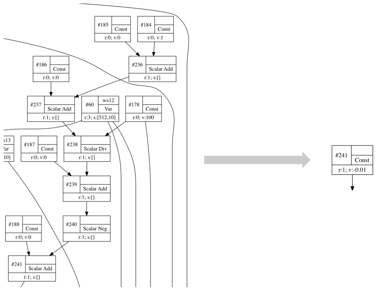
  Figure 5: Constant folding: node #241 depends only on constant nodes.

• Some patterns of nodes can be fused in order to be executed in a more efficient way. For instance, an FMA (fused-multiply-add) node can replace a multiplication followed by an addition to reduce memory access and improve numerical accuracy. A common subpattern of AdaGrad [DHS11], which is heavily used in neural network training, can also be fused into one node (see Figure 6).

  

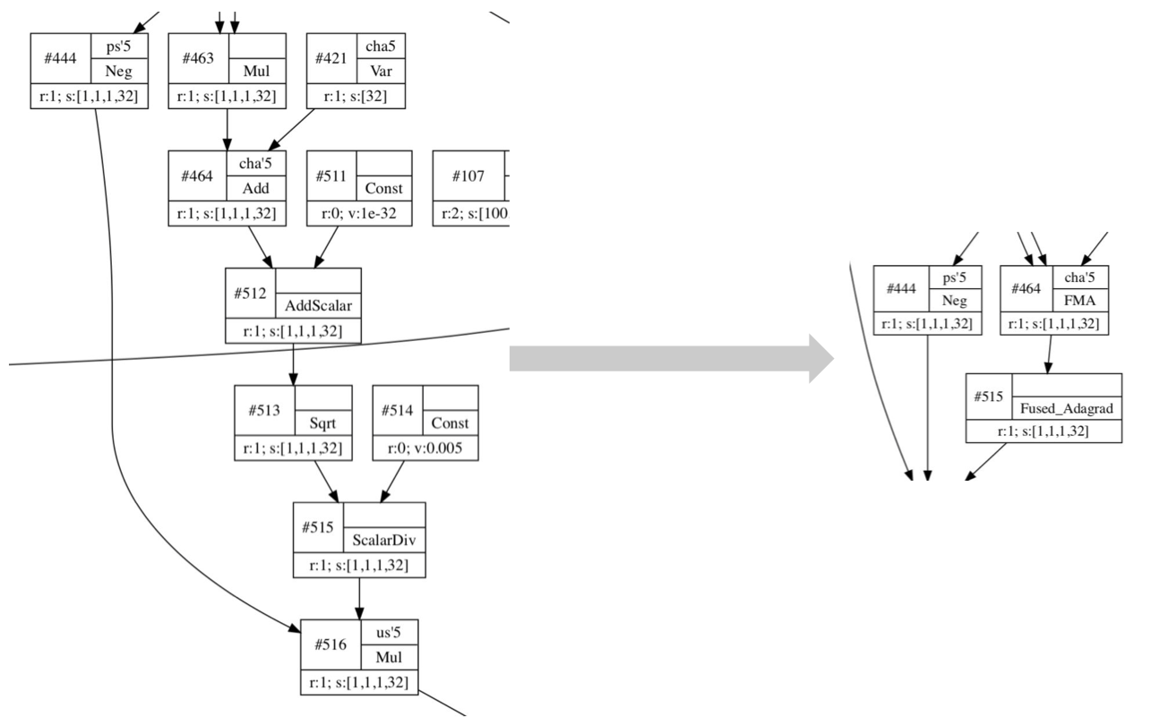
  Figure 6: Merging of #421, 463, 464 into FMA and of #511-516 into FusedAdagrad.

• Useless calculations, such as adding zero, dividing by one, multiplying by zero or one, repeating the input of an operation supporting broadcasting,… are automatically optimised.

Graph

This layer defines a graph type wrapping all the previous layers together. A graph is defined by its inputs and outputs nodes (from which the whole graph can be traversed). Inputs must be Var nodes and can be modified by the user before each evaluation. Graph visualisation functions are also provided. The mechanism to express the set of update edges $U$ from Definition 2.1 is a variable called iopair which should be specified when the graph is built. The function updateiopair activating this mechanism should be called at the end of each graph evaluation.

5 Device-dependant code

Owl’s computation graph currently supports both CPU and GPU devices. The GPU engine is based on OpenCL [SGS10]. We outline here the necessary parts to permit computation graph evaluation on a device.

5.1 Device

At the bottom of the functor stack, the Device layer abstracts implementation details about how tensors and scalar values are handled by the device. This is straightforward to implement for CPU devices — a tensor is simply a contiguous block in memory. On GPUs, tensors require a host (CPU) memory and a device (GPU) memory, plus a way to synchronise them.

5.2 Initialisation

Each device stores values in a different way, thus memory initialisation is device-dependant. We have seen that the ability to preallocate memory for each vertex is one of the main advantages of using a computation graph. Compared to the pebble game (Definition 3.1), we need to be careful of a few more caveats.

• Some operations, dependently on how they are implemented, can not overwrite some of their parents while they are being carried out. In the pebble game, this corresponds to forbidding the sliding of one pebble for some operators.

• We need to take into account that some vertices have different output sizes. In the pebble game, this means that we want to assign to each pebble a size that must be larger than the output size of the vertices the pebble is placed on. What we actually want to minimise is the sum of the sizes of the pebbles rather than the number of pebbles (this is still equivalent to the original problem in the specific case where all the output sizes are equal).

• We want to always keep the value of some vertices in memory for practical purposes (for example, vertices $v$ such that $\lambda(v)=\texttt{Const}$, output vertices, vertices $u$ such that $(u,v)\in U$). In Owl, a boolean value is used to indicate whether the memory of a vertex can be reused.

We explain in more detail the memory allocation performed in Owl when running the code on a CPU device. For practical reasons, since the algorithm should be efficient for arbitrary graphs, we assume that each vertex can only be computed once (i.e. keeping a minimal time value). The chosen algorithm is inspired by the one used by MXNet [CLL⁺15].

A first challenge is to find an efficient way to share memory between vertices which do not have the same output size. Since Owl’s multi-dimensional array module is based on OCaml’s Bigarray, we can use the reshape and subleft functions in the following way:

⬇

module N = Owl.Dense.Ndarray.S

let block = N.empty [|block_size|] in

let memory =

N.reshape (N.sub_left block 0 node_numel) shape

The block variable is a one-dimensional array of sufficient size. We reuse the nodenumel first elements of block and reshape that one-dimensional array to the right shape. Multiple nodes can thus base their memory on the same block, as long as their size is smaller than the size of the block, with no loss of performance.

The topological ordering $\gamma$ we use for allocation and evaluation is given by traversing the graph from the outputs using a post-order DFS.

By going through $\gamma$ in order, we can notice when the memory of a vertex becomes useless by keeping a counter of the number of times its value has been used by one of its successors. When all its successors have been evaluated, the memory block of the vertex can be tagged as reusable.

We follow the rules below to allocate a block of memory to a vertex $v$:

• we only allocate a new block when no block is available;

• when multiple blocks are available, we pick the smallest block that is big enough to contain the value of $v$, so that as little memory as possible stays unused. If the available blocks are all smaller that $v$, we increase the size of the current biggest block to fit $v$;

• when possible, we always favour an inplace reuse (i.e. reusing the memory of a direct predecessor of $v$) to reduce memory access overhead.

You can find the pseudo-code of the algorithm in Algorithm 1.

Algorithm 1 Memory Allocation for CPU devices

Variables

     $refs$, associating to each node its number of successors

     $reusable$, used to store the available blocks

     $block\_size$, associating to each block a size

     $block$, associating to each node a block

end Variables

function FindBestBlock($s$)

     if there is a block in $reusable$ with size $\geq s$ then

         return smallest block in $reusable$ of size $\geq s$

     else if $reusable$ is not empty then

         $b\leftarrow$ largest block in $block$

         $block\_size(b)\leftarrow s$

         return $b$

     else

         $b\leftarrow$ new block

         $block\_size[b]\leftarrow s$

         return $b$      

function Initialise($x$) Input: a node $x$ of the computation graph Effect: allocates a block of memory to $x$ and its ancestors.

     if $x$ is not initialised then

         for all predecessor $p$ of $x$ do Initialise($p$)          

         for all predecessor $p$ of $x$ do

              $ref[p]\leftarrow ref[p]-1$

              if $ref[p]=0$ then $reusable.add(p)$                        

         $block[x]\leftarrow$ FindBestBlock($size(x)$)      

The overall time complexity of the allocation is $\mathcal{O}(n*\log(b))$, where $n$ is the number of nodes in the graph and $b$ is the number of distinct memory blocks at the end of the algorithm (of course, $b\leq n$). The $\log(b)$ factor comes from the FindBestBlock function.

5.3 Evaluation

The device engine should also provide evaluation functions for all the operators defined in the Type functor, using functions defined in the selected Ndarray module.

6 Benchmarks

We show in Figure 7 the gain that can be obtained by using a computation graph in a few notorious neural network architectures, namely InceptionV3 [SLJ⁺15], ResNet [HZRS16], Mask R-CNN [HGDG17] (ported from implementation [Abd17]) and a small neural network solving the MNIST number classification .

Architecture	Time w/o	Time w/ CG (s)		Memory w/o	Memory w/
	CG (s)	Building	Evaluating	CG (MB)	CG (MB)
InceptionV3	0.5649	0.1066	0.2275	625.76	230.10
ResNet50	0.7933	0.1395	0.6090	1309.9	397.07
MNIST (training)	20.422	0.1436	10.920	3685.3	895.32
Mask R-CNN	11.538	0.3630	8.379	6483.4	870.48

Figure 7: InceptionV3 and ResNet50 are tested with a 299x299 image; Mask R-CNN is tested with a 768x768 image. The time is the average over 30 evaluations, without reusing pre-computed nodes when a computation graph is used. The graph building phase includes graph construction, optimisation and memory initialisation. The memory is the maximum resident set size of the program. This was evaluated on a laptop with an Intel i5-6300HQ CPU and 8 GB of RAM.

References

- [Abd17] Waleed Abdulla. Mask R-CNN for object detection and instance segmentation on Keras and TensorFlow. https://github.com/matterport/Mask_RCNN, 2017.
- [APW12] Per Austrin, Toniann Pitassi, and Yu Wu. Inapproximability of treewidth, one-shot pebbling, and related layout problems. In Anupam Gupta, Klaus Jansen, José Rolim, and Rocco Servedio, editors, Approximation, Randomization, and Combinatorial Optimization. Algorithms and Techniques, pages 13–24, Berlin, Heidelberg, 2012. Springer Berlin Heidelberg.
- [CLL+15] Tianqi Chen, Mu Li, Yutian Li, Min Lin, Naiyan Wang, Minjie Wang, Tianjun Xiao, Bing Xu, Chiyuan Zhang, and Zheng Zhang. MXNet: A flexible and efficient machine learning library for heterogeneous distributed systems. CoRR, abs/1512.01274, 2015.
- [CXZG16] Tianqi Chen, Bing Xu, Chiyuan Zhang, and Carlos Guestrin. Training deep nets with sublinear memory cost. CoRR, abs/1604.06174, 2016.
- [DHS11] John Duchi, Elad Hazan, and Yoram Singer. Adaptive subgradient methods for online learning and stochastic optimization. J. Mach. Learn. Res., 12:2121–2159, July 2011.
- [GLT79] John R. Gilbert, Thomas Lengauer, and Robert Endre Tarjan. The pebbling problem is complete in polynomial space. In Proceedings of the Eleventh Annual ACM Symposium on Theory of Computing, STOC ’79, pages 237–248, New York, NY, USA, 1979. ACM.
- [HGDG17] Kaiming He, Georgia Gkioxari, Piotr Dollár, and Ross B. Girshick. Mask R-CNN. 2017 IEEE International Conference on Computer Vision (ICCV), pages 2980–2988, 2017.
- [HZRS16] Kaiming He, Xiangyu Zhang, Shaoqing Ren, and Jian Sun. Deep residual learning for image recognition. In 2016 IEEE Conference on Computer Vision and Pattern Recognition, CVPR 2016, Las Vegas, NV, USA, June 27-30, 2016, pages 770–778. IEEE Computer Society, 2016.
- [LINK18] Tung D. Le, Haruki Imai, Yasushi Negishi, and Kiyokuni Kawachiya. TFLMS: Large model support in tensorflow by graph rewriting, 2018.
- [Nor13] Jakob Nordstrom. Pebble games, proof complexity, and time-space trade-offs. 2013.
- [Sav97] John E. Savage. Models of Computation: Exploring the Power of Computing. Addison-Wesley Longman Publishing Co., Inc., Boston, MA, USA, 1st edition, 1997.
- [Set73] Ravi Sethi. Complete register allocation problems. In Proceedings of the Fifth Annual ACM Symposium on Theory of Computing, STOC ’73, pages 182–195, New York, NY, USA, 1973. ACM.
- [SGS10] J. E. Stone, D. Gohara, and G. Shi. OpenCL: A parallel programming standard for heterogeneous computing systems. Computing in Science Engineering, 12(3):66–73, May 2010.
- [SLJ+15] Christian Szegedy, Wei Liu, Yangqing Jia, Pierre Sermanet, Scott Reed, Dragomir Anguelov, Dumitru Erhan, Vincent Vanhoucke, and Andrew Rabinovich. Going deeper with convolutions. In Computer Vision and Pattern Recognition (CVPR), 2015.
- [Wan17] Liang Wang. Owl: A general-purpose numerical library in OCaml. CoRR, abs/1707.09616, 2017.