Abduction-Based Explanations for Machine Learning Models

Abstract

The growing range of applications of Machine Learning (ML) in a multitude of settings motivates the ability of computing small explanations for predictions made. Small explanations are generally accepted as easier for human decision makers to understand. Most earlier work on computing explanations is based on heuristic approaches, providing no guarantees of quality, in terms of how close such solutions are from cardinality- or subset-minimal explanations. This paper develops a constraint-agnostic solution for computing explanations for any ML model. The proposed solution exploits abductive reasoning, and imposes the requirement that the ML model can be represented as sets of constraints using some target constraint reasoning system for which the decision problem can be answered with some oracle. The experimental results, obtained on well-known datasets, validate the scalability of the proposed approach as well as the quality of the computed solutions.

Introduction

The fast growth of machine learning (ML) applications has motivated efforts to validate the results of ML models (?; ?; ?; ?; ?; ?; ?), but also efforts to explain predictions made by such models (?; ?; ?; ?; ?; ?; ?; ?). One concern is the application of ML models, including Deep Neural Networks (DNNs) in safety-critical applications, and the need to provide some sort of certification about correctness of operation. The importance of computing explanations is further underscored by a number of recent works (?; ?; ?; ?; ?), by recent regulations (?), ongoing research programs (?), but also by recent meetings (?; ?; ?; ?).

For logic-based models, e.g. decision trees and sets, explanations can be obtained directly from the model, and related research work has mostly focused on minimizing the size of representations (?; ?). Nevertheless, important ML models, that include neural networks (NNs), support vector machines (SVMs), bayesian network classifiers (BNCs), among others, do not naturally provide explanations to predictions made. Most work on computing explanations for such models is based on heuristic approaches, with no guarantees of quality (?; ?; ?; ?; ?). Recent work (?) suggests that these heuristic approaches can perform poorly in practical settings. For BNCs, a recent compilation-based approach (?) represents a first step towards computing explanations with guarantees of quality. Nevertheless, a drawback of compilation approaches is the exponential worst-case size of the compiled representation, and also the fact that it is specific to BNCs.

This paper explores a different path, and proposes a principled approach for computing minimum explanations of ML models. Concretely, the paper exploits abductive reasoning for computing explanations of ML models with formal guarantees, e.g. cardinality-minimal or subset-minimal explanations. More importantly, our approach exploits the best properties of logic-based and heuristic-based approaches. Similar to heuristic approaches, our method is model-agnostic. If an ML model can be expressed in a suitable formalism then it can be explained in our framework. Similar to logic-based approaches, our method provides formal guarantees on the generated explanations. For example, we can generate cardinality-minimal explanations. Moreover, it allows a user to specify custom constraints on explanations, e.g. a user might have preferences over explanations. Although the use of abductive reasoning for computing explanations is well-known (?; ?), its application in explainable AI is novel to the best of our knowledge. The abductive reasoning solution is based on representing the ML model as a set of constraints in some theory (e.g. a decidable theory of first-order logic). The ML model prediction explanation approach proposed in this paper imposes mild requirements on the target ML model and the constraint reasoning system used. One must be able to encode the ML model as a set of constraints, and the constraint reasoning system must be able to answer entailment queries.

To illustrate the application of abductive reasoning for computing explanations, the paper focuses on Neural Networks. As a result, a recently proposed encoding of NNs into Mixed Integer Linear Programming is used (?). This encoding is also evaluated with Satisfiability Modulo Theories (SMT) solvers. Although other recently proposed MILP encodings could be considered (?), the most significant differences are in the algorithm used.

The experimental results, obtained on representative problem instances, demonstrate the scalability of the proposed approach, and confirm that small explanations can be computed in practice.

Background

Propositional Formulas, Implicants and Abduction.

We assume definitions standard in propositional logic and satifiability (?), with the usual definitions for (CNF) formulas, clauses and literals. Where required, formulas are viewed as sets of clauses, and clauses as sets of literals. For propositional formulas, a(n) (partial) assignment is a (partial) map from variables to $\mathbb{B}=\{0,1\}$. A satisfying assignment is such that the valuation of the formula (under the usual semantics of propositional logic) is 1. Throughout the paper, assignments will be represented as conjunctions of literals. Moreover, let $\mathcal{F}$ be a propositional formula defined on a set of variables $X=\{x_{1},\ldots,x_{n}\}$. A literal is either a variable $x_{i}$ or its complement $\neg x_{i}$. A term is a set of literals, interpreted as a conjunction of literals. A term $\pi$ is an implicant if $\pi\operatorname*{\vDash}\mathcal{F}$. An implicant $\pi$ is a prime implicant if $\pi\operatorname*{\vDash}\mathcal{F}$, and for any proper subset $\pi^{\prime}\subsetneq\pi$, $\pi^{\prime}\operatorname*{\nvDash}\mathcal{F}$ (?). A prime implicant $\pi$ given a satisfying assignment $\mu$ is any prime implicant $\pi\subseteq\mu$. Given a CNF formula and a satisfying assignment, a prime implicant can be computed in polynomial time. For an arbitrary propositional formula, given a satisfying assignment, a prime implicant can be computed with a linear number of calls to an NP solver (e.g. (?)). In contrast, computing the shortest prime implicant is hard for $\Sigma_{2}^{\textnormal{P}}$ (?), the second level of the polynomial hierarchy.

Let $\mathcal{F}$ denote a propositional theory which, for the goals of this paper can be understood as a set of clauses. Let $\mathcal{H}$ and $\mathcal{E}$ be respectively a set of hypotheses and a set of manifestations (or the evidence), which often correspond to unit clauses, but can also be arbitrary clauses.

A propositional abduction problem (PAP) is a 5-tuple $P=(\mathcal{V},\mathcal{H},\mathcal{E},\mathcal{F},c)$. $\mathcal{V}$ is a finite set of variables. $\mathcal{H}$, $\mathcal{E}$ and $\mathcal{F}$ are CNF formulas representing, respectively, the set of hypotheses, the set of manifestations, and the background theory. $c$ is a cost function associating a cost with each clause of $\mathcal{H}$, $c:\mathcal{H}\to\mathbb{R}^{+}$.

Given a background theory $\mathcal{F}$, a set $\mathcal{S}\subseteq\mathcal{H}$ of hypotheses is an explanation (for the manifestations) if: (i) $\mathcal{S}$ entails the manifestations $\mathcal{E}$ (given $\mathcal{F}$); and (ii) $\mathcal{S}$ is consistent (given $\mathcal{F}$). The propositional abduction problem consists in computing a minimum size explanation for the manifestations subject to the background theory, e.g. (?; ?; ?).

Definition 1 (Minimum-size explanations for $P$)

Let $P=(\mathcal{V},\mathcal{H},\mathcal{E},\mathcal{F},c)$ be a PAP. The set of explanations of $P$ is given by the set $\textnormal{Expl}(P)=\{\mathcal{S}\subseteq\mathcal{H}\>|\>\mathcal{F}\land\mathcal{S}\operatorname*{\nvDash}\bot,\mathcal{F}\land\mathcal{S}\operatorname*{\vDash}\mathcal{E}\}$. The minimum-cost solutions of $P$ are given by $\textnormal{Expl}_{c}(P)=\textnormal{argmin}_{E\in\textnormal{Expl}(P)}(c(E))$.

Subset-minimal explanations can be defined similarly. Moreover, throughout the paper the cost function assigns unit cost to each hypothesis, and so we use the following alternative notation for a PAP $P$, $P=(\mathcal{V},\mathcal{H},\mathcal{E},\mathcal{F})$.

First Order Logic and Prime Implicants.

We assume definitions standard in first-order logic (FOL) (e.g. (?)). Given a signature $\mathcal{S}$ of predicate and function symbols, each of which characterized by its arity, a theory $\mathcal{T}$ is a set of first-order sentences over $\mathcal{S}$. $\mathcal{S}$ is extended with the predicate symbol $=$, denoting logical equivalence. A model $\mathcal{M}$ is a pair $\mathcal{M}=(\mathcal{U},\mathcal{I})$, where $\mathcal{U}$ denotes a universe, and $\mathcal{I}$ is an interpretation that assigns a semantics to the predicate and function symbols of $\mathcal{S}$. A set $\mathcal{V}$ of variables is assumed, which is distinct from $\mathcal{S}$. A (partial) assignment $\nu$ is a (partial) function from $\mathcal{V}$ to $\mathcal{U}$. Assignments will be represented as conjunctions of literals (or cubes), where each literal is of the form $v=u$, with $v\in\mathcal{V}$ and $u\in\mathcal{U}$. Throughout the paper, cubes and assignments will be used interchangeably. The set of free variables in some formula $\mathcal{F}$ is denoted by $\textsl{free}(\mathcal{F})$. Assuming the standard semantics of FOL, and given an assignment $\nu$ and corresponding cube $C$, the notation $\mathcal{M},C\operatorname*{\vDash}\mathcal{F}$ is used to denote that $\mathcal{F}$ is true under model $\mathcal{M}$ and cube $C$ (or assignment $\nu$). In this case $\nu$ (resp. $C$) is referred to as satisfying assignment (resp. cube), with the assignment being partial if $|C|<|\mathcal{V}|$ (and so if $\nu$ is partial). A solver for some FOL theory $\mathcal{T}$ is referred to as a $\mathcal{T}$-oracle.

A well-known generalization of prime implicants to FOL (?) will be used throughout.

Definition 2

Given a FOL formula $\mathcal{F}$ with a model $\mathcal{M}=(\mathcal{U},\mathcal{I})$, a cube $C$ is a prime implicant of $\mathcal{F}$ if

1. $\mathcal{M},C\operatorname*{\vDash}\mathcal{F}$.

2. If $C^{\prime}$ is a cube such that $\mathcal{M},C^{\prime}\operatorname*{\vDash}\mathcal{F}$ and $\mathcal{M},C^{\prime}\operatorname*{\vDash}C$, then $\mathcal{M},C\operatorname*{\vDash}C^{\prime}$.

A smallest prime implicant is a prime implicant of minimum size. Smallest prime implicants can be related with minimum satisfying assignments (?). Finally, a prime implicant $C$ of $\mathcal{F}$ and $\mathcal{M}$ given a cube $C^{\prime}$ is a prime implicant of $\mathcal{F}$ such that $C\subseteq C^{\prime}$.

Satisfiability Modulo Theories (SMT) represent restricted (and often decidable) fragments of FOL (?). All the definitions above apply to SMT.

Mixed Integer Linear Programming (MILP).

In this paper, a MILP is defined over a set of variables $V$, which are partitioned into real (e.g. $Y$), integer (e.g. $W$) and Boolean (e.g. $Z$) variables.

$$\begin{array}[]{lll}\textnormal{min}&\sum_{v_{j}\in V}c_{j}v_{j}\\[5.0pt] \textnormal{s.t.}&\sum_{v_{j}\in V}a_{ij}v_{j}\leq b_{i}&1\leq i\leq K\\ \end{array}$$ (1)

where $\{b_{1},\ldots,b_{K}\}$ can either be real, integer or Boolean values. To help with the encoding of ML models, we will exploit indicator constraints (e.g. (?; ?)) of the form:

$$l_{i}\to\left(\sum_{v_{j}\in V}a_{ij}v_{j}\leq b_{i}\right)$$ (2)

where $l_{i}$ is some propositional literal.

Clearly, under a suitable definition of signature $\mathcal{S}$ and model $\mathcal{M}$, with $\mathcal{U}\triangleq\mathbb{R}\cup\mathbb{Z}\cup\mathbb{B}$, (smallest) prime implicants can be computed for MILP.

Minimal Hitting Sets.

Given a collection $\mathbb{S}$ of sets from a universe $\mathbb{U}$, a hitting set $h$ for $\mathbb{S}$ is a set such that $\forall S\in\mathbb{S},h\cap S\neq\emptyset.$ A hitting set $h$ is said to be minimal if none of its subsets is a hitting set.

ML Explanations as Abductive Reasoning

We consider the representation of an ML model using a set of constraints, represented in the language of some constraint reasoning system. Associated with this constraint reasoning system, we assume access to an oracle that can answer entailment queries. For example, one can consider Satisfiability Modulo Theories, Constraint Programming, or Mixed Integer Linear Programming.

Moreover, we associate the quality of an explanation with the number of specified features associated with a prediction. As a result, one of the main goals is to compute cardinality-minimal explanations. Another, in practice more relevant due to performance challenges of the first goal, is to compute subset-minimal explanations.

Propositional Case.

Let $\mathbb{M}$ denote some ML model. We assume a set of (binarized) features $\mathcal{V}=\{f_{1},\ldots,f_{k}\}$, and a classification problem with two classes $\{c_{0},c_{1}\}$. Let some $p\in\{c_{0},c_{1}\}$ denote some prediction. Moreover, let us assume that we can associate a logic theory $\mathcal{T}$ with the ML model $\mathbb{M}$, and encode $\mathbb{M}$ as a formula $\mathcal{F}$.

Given the above, one can compute cardinality minimal explanations for $p$ as follows. Let $\mathcal{H}=\{(f_{i}),(\neg f_{i})|f_{i}\in\mathcal{V}\}$, let $\mathcal{E}=\{(p)\}$, and associate a unit cost function $\nu$ with each unit clause of $\mathcal{H}$. Then, any explanation for the PAP $P=(\mathcal{V},\mathcal{H},\mathcal{E},\mathcal{F})$ is an explanation for the prediction $p$. To compute cardinality minimal explanations, we can use for example a recently proposed approach (?). Moreover, observe that if features are real-valued, then the approach outlined above for computing cardinality minimal explanations does not apply.

In a more concrete setting of some point $\phi$ in feature space and prediction $p$, we consider a concrete set $\mathcal{H}$, where the value of each feature of $\phi$ is represented with a unit clause. As above, we can consider propositional abduction, which in this case corresponds to computing the (minimum-size) prime implicants that explain the prediction as a subset of the point in feature space. This relationship is detailed next.

General Case.

In a more general setting, features can take arbitrary real, integer or Boolean values. In this case we consider an input cube $C$ and a prediction $\mathcal{E}$. The relationship between abductive explanations and prime implicants is well-known (e.g. (?; ?). Let $C$ be the cube associated with some satisfying assignment. Regarding the computation of abductive explanations, $C\land\mathcal{F}\operatorname*{\nvDash}\bot$ and the same holds for any subset of $C$. This means that we just need to consider the constraint $C\land\mathcal{F}\operatorname*{\vDash}\mathcal{E}$, which is equivalent to $C\operatorname*{\vDash}(\mathcal{F}\to\mathcal{E})$. Thus, a subset-minimal explanation $C_{m}$ (given $C$) is a prime implicant of $\mathcal{F}\to\mathcal{E}$ (given $C$), and a cardinality-minimal explanation $C_{M}$ (given $C$) is a cardinality-minimal prime implicant of $\mathcal{F}\to\mathcal{E}$ (given $C$). Thus, we can compute subset-minimal (resp. cardinality-minimal) explanations by computing instead prime implicants (resp. shortest PIs) of $\mathcal{F}\to\mathcal{E}$. As a final remark, the cardinality minimal prime implicants of $\mathcal{F}\to\mathcal{E}$ are selected among those that are contained in $C$.

Computing Explanations.

This section outlines the algorithms for computing a subset-minimal explanation and a cardinality-minimal explanation. The computation of a subset-minimal explanation requires a linear number of calls to a $\mathcal{T}$-oracle. In contrast, the computation of a cardinality-minimal explanation in the general case requires a worst-case exponential number of calls to a $\mathcal{T}$-oracle (?).

1

2

Input:     $\mathcal{F}$ under $\mathcal{M}$, initial cube $C$, prediction $\mathcal{E}$

Output: Subset-minimal explanation $C_{m}$

3 begin

4      foreach $l\in C$ do

5            if $\textnormal{{Entails}}(C\setminus\{l\},\mathcal{F}\rightarrow\mathcal{E},\mathcal{M})$ then

6                  $C\leftarrow C\setminus\{l\}$

7           

8     return $C$

9     

10      end

11     

Algorithm 1 Computing a subset-minimal explanation

Algorithm 1 shows the algorithm to compute a subset-minimal explanation for a prediction $\mathcal{E}$ made by an ML model $\mathbb{M}$ encoded into formula $\mathcal{F}$ under model $\mathcal{M}$. Given a cube $C$ encoding a data sample for the prediction $\mathcal{E}$, the procedure returns its minimal subset $C_{m}$ s.t. $\mathcal{F}\land C_{m}\operatorname*{\vDash}\mathcal{E}$ under $\mathcal{M}$. Based on the observation made above, Algorithm 1 iteratively tries to remove literals $l$ of the input cube $C$ followed by a check whether the remaining subcube is an implicant of formula $\mathcal{F}\rightarrow\mathcal{E}$, i.e. $(C\setminus\{l\})\operatorname*{\vDash}(\mathcal{F}\rightarrow\mathcal{E})$. Note that to check the entailment, it suffices to test whether formula $(C\setminus\{l\})\land\mathcal{F}\land\neg{\mathcal{E}}$ is false. As a result, the algorithm traverses all literals of the cube and, thus, makes $|C|$ calls to the $\mathcal{T}$-oracle.

1

2

3

Input:     $\mathcal{F}$ under $\mathcal{M}$, initial cube $C$, prediction $\mathcal{E}$

Output: Cardinality-minimal explanation $C_{M}$

4 begin

5      $\Gamma\leftarrow\emptyset$

6      while true do

7            $h\leftarrow\textnormal{{MinimumHS}}(\Gamma)$

8            if $\textnormal{{Entails}}(h,\mathcal{F}\rightarrow\mathcal{E},\mathcal{M})$ then

9                 return $h$

10           else

11                  $\mu\leftarrow\textnormal{{GetAssignment}}()$

12                  $C^{\prime}\leftarrow\textnormal{{PickFalseLits}}(C\setminus h,\mu)$

13                  $\Gamma\leftarrow\Gamma\cup C^{\prime}$

14                 

15           

16     

17      end

18     

Algorithm 2 Computing a smallest size explanation

Computing a cardinality-minimal explanation is hard for $\Sigma_{2}^{\textnormal{P}}$ (?) and so it is practically less efficient to perform. For the propositional case, a smallest size explanation can be extracted using directly a propositional abduction solver (?) applied to the setup described above. Note that in the general case dealing with FOL formulas, the number of all possible hypotheses is infinite and so a similar setup is not applicable. However, and analogously to Algorithm 1, one can start with a given cube $C$ representing an input data sample and consistent with formula $\mathcal{F}$ representing an ML model.

Algorithm 2 shows a pseudo-code of the procedure computing a smallest size explanation for prediction $\mathcal{E}$. The algorithm can be seen as an adaptation of the propositional abduction approach (?) to the general ML explanation problem and is based on the implicit hitting set paradigm. As such, Algorithm 2 is an iterative process, which deals with a set $\Gamma$ of the sets to hit. Initially, set $\Gamma$ is empty (line 2). At each iteration, a new smallest size hitting set $h$ for $\Gamma$ is computed (see line 2). Hitting set $h$ is then treated as a cube, which is tested on whether it is a prime implicant of formula $\mathcal{F}\rightarrow\mathcal{E}$ under model $\mathcal{M}$. As was discussed above, this can be tested by calling a $\mathcal{T}$-oracle on formula $h\land\mathcal{F}\land\neg{\mathcal{E}}$ (line 2). If the $\mathcal{T}$-oracle returns false, the algorithm reports hitting set $h$ as a smallest size explanation for the prediction and stops. Otherwise, i.e. if the $\mathcal{T}$-oracle returns true, an assignment $\mu$ for the free variables of formula $h\land\mathcal{F}\land\neg{\mathcal{E}}$ is extracted (see line 2). Assignment $\mu$ is then used to determine a subset $C^{\prime}$ of literals of cube $C\setminus h$ that were falsified by the previous call to the $\mathcal{T}$-oracle. Finally, set $\Gamma$ is updated on line 2 to include $C^{\prime}$ and the process continues.

Note that the correctness of Algorithm 2, although not proved here, immediately follows from the correctness of the original hitting set based approach to propositional abduction (?). The intuition behind the algorithm is the following. Every iteration checks whether a given (smallest size) subset $h$ of the input cube $C$ is an implicant of $\mathcal{F}\rightarrow\mathcal{E}$. If this is not the case, some other literals, i.e. from set $C\setminus h$, should be included to $h$ at the next iteration of the algorithm. Moreover, a new set $C^{\prime}$ to hit comprises only literals of $C\setminus h$ that were falsified during the previous $\mathcal{T}$-oracle call because they are guaranteed to have been disabled previously, not only by our choice of $h$ but also by the $\mathcal{T}$-oracle call.

Example 1

Consider an example model mapping pairs of all possible integers $i_{1}$ and $i_{2}$ into set $\{1,2\}$. Assume the model is encoded to the following set of (indicator) constraints $\mathcal{F}$ given variables $z_{k}\in\{0,1\}$, $k\in[3]$:

$z_{1}=1\leftrightarrow i_{1}\leq 0,\,\,z_{3}=1\leftrightarrow z_{1}+z_{2}\leq 1,\,\,z_{3}=1\rightarrow o=1$

$z_{2}=1\leftrightarrow i_{2}\leq 0,\;\;\;\;\;\;\;\;\;\;\;\;\;\;\;\;\;\;\;\;\;\;\;\;\;\;\;\;\;\;\;\;\;\;\;\,z_{3}=0\rightarrow o=2$

Given a data sample encoded as a cube $C=(i_{1}=3)\land(i_{2}=2)$, the prediction is $1$. It is clear that there are two minimal explanations for this classification: $C_{m}^{1}=(i_{1}=3)$ and $C_{m}^{2}=(i_{2}=2)$. Observe that both can be trivially computed by the linear search procedure of Algorithm 1 because $C_{m}^{j}\operatorname*{\vDash}(\mathcal{F}\rightarrow(o=1))$ is true for $j\in[2]$.

Encoding Neural Networks with MILP

This section considers a MILP encoding of a neural network with a commonly-used ‘rectified linear unit’ nonlinear operator (ReLU). For simplicity, we explain an encoding of a building block of the network as all blocks have the same structure and are assembled sequentially to form the network. A block consists of a linear transformation and a non-linear transformation. Let $x=\{x_{1},\ldots,x_{n}\},x\in\mathbb{R}^{n}$ be an input and $y=\{y_{1},\ldots,y_{m}\}\in\mathbb{R}_{\geq 0}^{m}$ be an output of a block. First, we apply a linear transformation $x^{\prime}=Ax+b$, where $A\in\mathbb{R}^{m}\times\mathbb{R}^{n}$ and $b\in\mathbb{R}^{m}$ are real-valued parameters of the network. Then we apply a non-linear transformation $y=\mbox{\sc ReLU}(x^{\prime})$, where $\mbox{\sc ReLU}=\mbox{max}(x^{\prime},0)$.

To encode a block, we use a recently proposed MILP encoding (?). One useful modeling property of this encoding is that it employs indicator constraints that are natively supported by modern MILP solvers. Hence, we can avoid using the Big-M notation in the encoding that requires good bounds tightening to compute the value of Big-M. To perform the encoding, we introduce two sets of variables: Boolean variables $z=\{z_{1},\ldots,z_{m}\},z\in\{0,1\}^{m}$ and auxiliary real variables $s=\{s_{1},\ldots,s_{m}\},s\in\mathbb{R}_{\geq 0}^{m}$. Intuitively, the $z_{i}$ variable encodes the sign of $\sum_{j=1}^{n}a_{i,j}x_{j}+b_{i}$. If $z_{i}=1$ then $\sum_{j=1}^{n}a_{i,j}x_{j}+b_{i}\leq 0$ and $y_{i}=0$. If $z_{i}=0$ then $\sum_{j=1}^{n}a_{i,j}x_{j}+b_{i}\geq 0$ and $y_{i}=\sum_{j=1}^{n}a_{i,j}x_{j}+b_{i}$. A block is encoded as follows:

$$\sum_{j=1}^{n}a_{i,j}x_{j}+b_{i}=y_{i}-s_{i},$$ (3)

$$z_{i}=1\rightarrow y_{i}\leq 0,$$ (4)

$$z_{i}=0\rightarrow s_{i}\leq 0,$$ (5)

$$y_{i}\geq 0,s_{i}\geq 0,z_{i}\in\{0,1\},$$ (6)

where $i\in[1,m]$. To see why the encoding is correct we consider two cases. First, we consider the case $z_{i}=1$. As we mentioned above, $y_{i}$ must be zero in this case. Indeed, if $z=1$ then $y_{i}\leq 0$ holds. Together with $y_{i}\geq 0$, we get that $y_{i}=0$. Similarly, $z_{i}=0$ should ensure that $\sum_{j=1}^{n}a_{i,j}x_{j}+b_{i}=y_{i}$. If $z=0$ then $s_{i}\leq 0$ forcing $s_{i}=0$. In this case, $y_{i}$ equals to $\sum_{j=1}^{n}a_{i,j}x_{j}+b_{i}$.

A common neural network architecture for classification problems performs a normalization of the network output as the last layer, e.g. the softmax layer. However, we do not need to encode this normalization transformation as it does not change the maximum value of the output that defines prediction of the network.

Example 2

Consider an example of a block with two inputs, $x_{1}$ and $x_{2}$ and two outputs $y_{1}$ and $y_{2}$. Let $A=[2,-1;1,1]$ and $b=[-1,1]$ be parameters of a linear transformation. To encode this block, we introduce auxiliary variables $s_{1}$, $s_{2}$, $z_{1}$ and $z_{2}$. We obtain the following constraints:

$$2x_{1}-x_{2}-1=y_{1}-s_{1},$$

$$x_{1}+x_{2}+1=y_{2}-s_{2},$$

$$z_{1}=1\rightarrow y_{1}\leq 0,z_{2}=1\rightarrow y_{2}\leq 0,$$

$$z_{1}=0\rightarrow s_{1}\leq 0,z_{2}=0\rightarrow s_{2}\leq 0,$$

$$y_{1}\geq 0,y_{2}\geq 0,s_{1}\geq 0,s_{2}\geq 0,z_{1}\in\{0,1\},z_{2}\in\{0,1\}.$$

Experimental Results

This section evaluates the scalability of the proposed approach to computing cardinality- and subset-minimal explanations and the quality of the computed explanations (in terms of the minimality guarantees). The benchmarks considered include the well-known text-based datasets from the UCI Machine Learning Repository and Penn Machine Learning Benchmarks, as well as the widely used MNIST digits database.

Setup and prototype implementation.

To assess scalability, all benchmarks were ran on a Macbook Pro having an Intel Core i7 2.8GHz processor with 8GByte of memory on board. Time limit was set to 1800 seconds while memory limit was set to 4GByte. The prototype implementation of the proposed approach follows Algorithm 1 and Algorithm 2 for computing subset- and cardinality-minimal explanations, respectively. It is written in Python and targets both SMT and MILP solvers. SMT solvers are accessed through the PySMT framework (?), which provides a unified interface to SMT solvers like CVC4, MathSAT5, Yices2, and Z3 among a few others. Note that in the following only the results of Yices2 (?) are shown as of the best performing SMT solver, selected based on a prior experimentation with CVC4, MathSAT5, Yices2, and Z3. CPLEX 12.8.0 (?) is used as a MILP oracle accessed via its official Python API. The implementation of minimum hitting set enumeration in Algorithm 2 is based on an award-winning maximum satisfiability solver RC2 written on top of the PySAT toolkit (?).

Quality of explanations.

This section focuses on a selection of datasets from UCI Machine Learning Repository and Penn Machine Learning Benchmarks (see Table 1 for details). The selected datasets have 9–32 features and contain 164–691 data samples. The experiment is organized as follows. First, given a dataset, a neural network is trained and encoded as described above. Second, the explanation procedure (computing either a subset- or a cardinality-minimal explanation) is ran for each sample of the dataset. If all samples get explained within 1800 seconds in total, the procedure is deemed to succeed. Otherwise, the process is interrupted meaning that the explanations for some of the samples are not extracted successfully.

Column 1 of Table 1 lists the selected datasets followed by the number of features. Column 4 details the minimal, average, and maximal size of explanations per sample for a given a dataset (depending on prefix m, a, and M in column 3). Analogously, columns 5–9 depict the minimal, average, and maximal time spent for computing an explanation for a given dataset, either with an SMT or a MILP oracle in use.

As one can observe, using a MILP oracle is preferred as it consistently outperforms its SMT rival. In general, the MILP-based solution is able to compute a subset-minimal explanation of a sample in a fraction of a second. Also note that subset- and cardinality-minimal explanation size varies a lot depending on the dataset. On the one hand, it may be (see australian) enough to keep just 1 feature to explain the outcome, which is $\approx 7\%$ of the data sample. On the other hand, some data samples cannot be reduced at all (see the M values in column 4). On average, the relative size of subset-minimal explanations varies from $28.5\%$ to $86.7\%$ with the mean value being $60.5\%$. This is deemed to provide a reasonable reduction of sample size, which may help a human interpret the outcomes of a machine learning classifier.

Table 1: Subset-minimal and cardinality-minimal explanations for the selected UCI and PennML datasets. Explanations are computed with the use of an SMT or a MILP oracle. The data shows minimal (m), average (a), and maximal (M) size of the computed explanations per dataset, as well as minimal (m), average (a), and maximal (M) time per dataset required to extract one explanation either by an SMT oracle or its MILP counterpart.

Dataset Minimal explanation Minimum explanation size SMT (s) MILP (s) size SMT (s) MILP (s) australian ($14$) m $1$ $0.03$ $0.05$ — — — a $8.79$ $1.38$ $0.33$ — — — M $14$ $17.00$ $1.43$ — — — auto ($25$) m $14$ $0.05$ $0.19$ — — — a $19.99$ $2.69$ $0.36$ — — — M $25$ $37.38$ $0.76$ — — — backache ($32$) m $13$ $0.13$ $0.14$ — — — a $19.28$ $5.08$ $0.85$ — — — M $26$ $22.21$ $2.75$ — — — breast-cancer ($9$) m $3$ $0.02$ $0.04$ $3$ $0.02$ $0.03$ a $5.15$ $0.65$ $0.20$ $4.86$ $2.18$ $0.41$ M $9$ $6.11$ $0.41$ $9$ $24.80$ $1.81$ cleve ($13$) m $4$ $0.05$ $0.07$ $4$ — $0.07$ a $8.62$ $3.32$ $0.32$ $7.89$ — $5.14$ M $13$ $60.74$ $0.60$ $13$ — $39.06$ cleveland ($13$) m $7$ — $0.07$ $7$ — $0.07$ a $9.23$ — $0.34$ $8.92$ — $2.03$ M $13$ — $1.02$ $13$ — $12.25$ glass ($9$) m $4$ $0.02$ $0.05$ $4$ $0.02$ $0.05$ a $7.82$ $0.18$ $0.15$ $7.68$ $1.13$ $0.29$ M $9$ $3.26$ $0.38$ $9$ $15.47$ $2.48$ glass2 ($9$) m $2$ $0.02$ $0.05$ $2$ $0.02$ $0.04$ a $5.20$ $0.47$ $0.15$ $4.51$ $3.31$ $0.74$ M $9$ $1.42$ $0.38$ $9$ $10.98$ $2.21$ heart-statlog ($13$) m $3$ $0.01$ $0.05$ $3$ $0.01$ $0.03$ a $8.13$ $0.13$ $0.15$ $7.09$ $1.51$ $1.01$ M $13$ $0.89$ $0.38$ $13$ $8.16$ $8.12$ hepatitis ($19$) m $6$ $0.02$ $0.04$ $4$ $0.01$ $0.04$ a $11.42$ $0.07$ $0.06$ $9.39$ $4.07$ $2.89$ M $19$ $0.26$ $0.20$ $19$ $27.05$ $22.23$ voting ($16$) m $3$ $0.01$ $0.02$ $3$ $0.01$ $0.02$ a $4.56$ $0.04$ $0.13$ $3.46$ $0.3$ $0.25$ M $11$ $0.10$ $0.37$ $11$ $1.25$ $1.77$ spect ($22$) m $3$ $0.02$ $0.02$ $3$ $0.02$ $0.04$ a $7.31$ $0.13$ $0.07$ $6.44$ $1.61$ $0.67$ M $20$ $0.88$ $0.29$ $20$ $8.97$ $10.73$

Subset- vs. cardinality-minimal explanations.

Compared to subset-minimal explanations, computing smallest size explanations is significantly more expensive due to the problem being hard for the second level of the polynomial hierarchy. As one can observe, the proposed explanation procedure fails to explain all data samples within the given total 1800 seconds (see australian, auto, backache). As in the case of minimal explanations, the MILP oracle outperforms the SMT-based solver being able to explain 2 more datasets. The size of smallest size explanations varies from $21.6\%$ to $85.3\%$ with the average value being $52.6\%$. Although cardinality-minimal explanations are in general smaller than subset-minimal ones, their computation takes a lot more time and so the overall advantage of minimum size explanations seems questionable.

State-of-the-art in logic-based explanations.

As a side problem, here we compare the quality of explanations produced by the current approach with the state of the art in logic-based explanation of Bayesian network classifiers (?), given a concrete dataset. Following (?), let us focus on the Congressional Voting Records dataset (referred to as voting in Table 1). The dataset contains 16 key votes by Congressmen of the U.S. House of Representatives, expressed as Boolean yes and no (1 and 0). Consider the following list of votes classified as Republican:

(0 1 0 1 1 1 0 0 0 0 0 0 1 1 0 1)

The BDD-based approach of (?) for explaining Bayesian network classifiers computes the following smallest size explanations of size 9:

(    0 1 1   0 0 0       1 1 0  )

(    0 1 1 1   0 0       1 1 0  )

To be able to compare to this data, we trained 4 neural networks separately of each other and tried to “explain” their predictions given this concrete data sample. As a result, we got the following subset-minimal explanations of size varying from 3 to 5:

(      1         0   0       0  )

(      1         0   0          )

(    0 1         0   0       0  )

(    0 1         0   0         1)

A possible intuition behind this impressive result is that models based on neural networks may generalize better than solutions relying on Bayesian networks and/or they allow for more “aggressive” and, thus, more efficient interpretation.

It should also be noted that the proposed approach is constraint-agnostic and computes explanations “of the fly” in the online manner while the work of (?) relies on prior compilation of the classifier function into a BDD, which is in general known to be computationally expensive.

Scalability and MNIST digits.

A widely used benchmark dataset for testing machine learning models is MNIST digits, which comprises a set of greyscale images depicting hand-written digits. This section aims at illustrating visually and discussing a few minimal explanations provided for example predictions of a neural network trained on the MNIST digits datasets. Concretely, let us consider a neural network with one hidden layer containing 15 or 20 neurons trained to distinguish two digits, e.g. 1 and 3, or 1 and 7, among other pairs. Each MNIST data sample describes a picture of size $\text{28}\times\text{28}$, and so the total number of features is 784.

Observe that the number of features makes these datasets significantly more challenging for extracting explanations. Our experiments confirm this fact as the average time spent for computing one subset-minimal explanation using a MILP oracle is about $52.86$ seconds. As for SMT, given 1 hour time limit, we were unable to get an explanation for any MNIST data sample using the SMT solvers available in PySMT. The average size of subset-minimal explanations varies from $46.4\%$ to $80.3\%$ of the total number of pixels (i.e. $784$), with the mean value being $63.92\%$. Also note that no cardinality-minimal explanation was computed within 1 hour time limit. This holds for all SMT and MILP alternatives tried.

(a)

(b)

(c)

(d)

Figure 1: Possible minimal explanations for digit one.

(a)

(b)

(c)

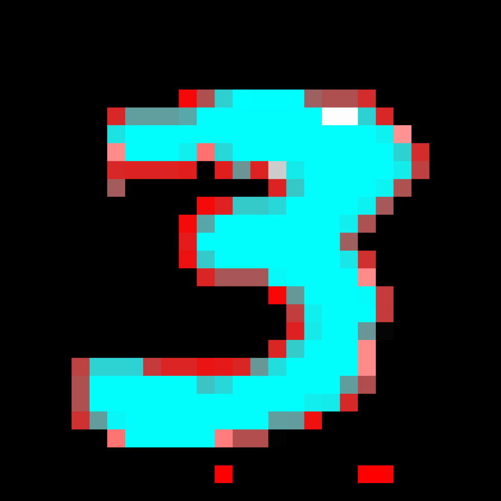
(d)

Figure 2: Possible minimal explanations for digit three.

Let us focus on two particular data samples shown in Figure 1(a) and Figure 2(a). These samples describe concrete ways of writing digits 1 and 3. Subset-minimal explanations for these samples computed by Algorithm 1 are depicted in Figure 1(b) and Figure 2(b), respectively. (Observe that pixels included in the explanations are either red or magenta while greyscale parts of the images are excluded from the explanations.) Note that Algorithm 1 tries to remove pixels from an image one by one starting from the top left corner and ending at the bottom right corner. As shown in Figure 1(b) and Figure 2(b), this procedure ends up keeping the bottom part of the image as it is needed to forbid misclassifications while the top part of the image being removed. While this is perfectly correct from the logical perspective, it may not satisfy some users as it does not give any reasonable hint on why the image is classified that specific way.

In this situation, better results could be obtained if the pixels were traversed in a different order. For instance, one may find reasonable first to remove pixels that are far from the image center because the most important information in an image is typically located close to its center. Applying this strategy to the considered samples results in the explanations highlighted in Figure 1(c) and Figure 2(c).

Another possible policy would be to prefer removing dark parts of an image keeping the light parts. The result of applying this policy is shown in Figure 1(d) and Figure 2(d). Moreover, a user may consider other heuristics to sort the pixels including various combinations of the ones described above. As there can be myriads of possible explanations for the same data sample, trying various heuristics to sort/order the pixels can help obtaining explanations that are more interpretable than the other from a human’s point of view.

Summary.

As shown above, the proposed approach for computing subset- and cardinality-minimal explanations for ML models using an underlying constraints formalism can obtain high quality results for a variety of popular datasets, e.g. from UCI Machine Learning Repository, Penn Machine Learning Benchmarks, and also MNIST digits. In particular, the experimental results indicate that the approach, if applied to neural network classifiers, is capable of obtaining explanations that are reasonably smaller than those of the state of the art and, thus, may be preferred as more interpretable from the point of view of human decision makers.

Scalability of the proposed ideas was tested with the use of SMT and MILP oracles. As it was shown, MILP in general outperforms its SMT counterparts. It was also shown that computing smallest-size explanations is computationally quite expensive, which makes subset-minimal explanations a better alternative. Another important factor here is that subset-minimal explanations are usually just a bit larger than cardinality-minimal explanations.

Related Work

We briefly overview two lines of research on heuristic-based explanations of machine learning models. The first line focuses on explaining a complex ML model as a whole using an interpretable model (?; ?). Such algorithms take a pair of ML models, an original complex ML model and a target explainable model, as an input. For example, the original model may be a trained neural network, and the target model may be a decision tree (?). One of the underlying assumptions here is that there exists a transformation from the original model to the target model that preserves the accuracy of the original model. The second line of work focuses on explanations of an ML model for a given input (?; ?; ?). For example, given an image of a car, we might want an explanation why a neural network classifies this image as a car. The most prominent example is the LIME framework (?). The main idea of the method is to learn important features of the input using its local perturbations. The algorithm observes how the ML model behaves on perturbed inputs. Based on this information, important features for the classification of a given sample are linearly separated from the rest of the features. The LIME method is model agnostic, as it can work with any ML model. Another group of methods is based on the saliency map (?). The idea is that the most important input features can be obtained using the knowledge of the ML model, e.g. gradients. However, none of these approaches provides any guarantees on the quality of explanations.

Discussion and Future Work

This paper proposes a principled approach to the problem of computing explanations of ML models. Nevertheless, the use of abductive reasoning, and the associated complexity, can raise concerns regarding robustness and scalability. Several ways can be envisioned to tackle the robustness issue. First, the approach enables a user not only to compute one explanation, either minimal or minimum, but also to enumerate a given number of such explanations. Second, since the proposed approach is based on calls to some oracle, preferences over explanations, e.g. in terms of (in)dependent feature weights, can in principle be accommodated.

Regarding the issue of scalability, it should be noted that developed prototype serves as a proof of concept that the proposed generic approach can provide small and reasonable explanations, which are arguably easier to understand by a human decision maker, this despite the underlying ML model being a blackbox, whose decisions may look uninterpretable per se. As the experimental results show, this holds for all the benchmark sets studied. Moreover and as the experimental results suggest, the approach still applies (with no conceptual modification) if one opts to use oracles other than an ILP solver (?; ?; ?; ?). Given the performance results obtained by these recent works, one should expect to be able to handle larger-scale NNs. Furthermore, since the proposed approach is constraint-agnostic, the same ideas can provide the basis for the the development of efficient decision procedures and effective encodings, not only for NN-based classifiers, but also for other state-of-the-art machine learning models. An alternative way to improve scalability would be to apply abstraction refinement techniques, a prominent approach that proved invaluable in many other settings.

Although the scalability of approaches for computing explanations is an important issue, the existence of a principled approach can serve to benchmark other heuristic approaches proposed in recent work (?; ?). More importantly, the proposed principled approach can elicit new heuristic approaches, that scale better than the exact methods outlined in the paper, but which in practice perform comparably to those exact methods. Observe also that explanations provided by any heuristic approach can, not only be validated, but can also be minimized further, in case additional minimization can be achieved.

As a final remark, note that by providing a high-level description, independent of a concrete ML model, the paper shows how the same general approach can be applied to any ML model that can be represented with (first-order logic) constraints. This demonstrates the flexibility of the proposed solution in that most existing ML models can (at least conceptually) be encoded with FOL. We emphasize that the approach is perfectly general. If for some reason FOL is inadequate to encode some ML model, one could consider second-order or even higher order logics. Of course, the price to pay would be the (potential) issues with decidability and scalability.

Conclusions

Explanations of ML predictions are essential in a number of applications. Past work on computing explanations for ML models has mostly addressed heuristic approaches, which can yield poor quality solutions. This paper proposes the use of abductive reasoning, namely the computation of (shortest) prime implicants, for finding subset- or cardinality-minimal explanations. Although the paper considers MILP encodings of NNs, the proposed approach is constraint-agnostic and independent of the ML model used. A similar approach can be applied to any other ML model, provided the model can be represented with some constraint reasoning system and entailment queries can be decided with a dedicated oracle. The experimental results demonstrate the quality of the computed explanation, and highlight an important tradeoff between subset-minimal explanations, which are computationally easier to find, and cardinality-minimal explanations, which can be far harder to find, but which offer the best possible quality (measure as the number of specified features).

A number of lines of work can be envisioned. These include considering other ML models, other encodings of ML models, other approaches for answering entailment queries, and also the evaluation of additional benchmark suites.

References

- [Al-Shedivat, Dubey, and Xing 2018] Al-Shedivat, M.; Dubey, A.; and Xing, E. P. 2018. The intriguing properties of model explanations. CoRR abs/1801.09808.
- [Angelino et al. 2017] Angelino, E.; Larus-Stone, N.; Alabi, D.; Seltzer, M.; and Rudin, C. 2017. Learning certifiably optimal rule lists. In KDD, 35–44.
- [Baehrens et al. 2010] Baehrens, D.; Schroeter, T.; Harmeling, S.; Kawanabe, M.; Hansen, K.; and Müller, K. 2010. How to explain individual classification decisions. Journal of Machine Learning Research 11:1803–1831.
- [Barrett et al. 2009] Barrett, C. W.; Sebastiani, R.; Seshia, S. A.; and Tinelli, C. 2009. Handbook of Satisfiability. IOS Press. chapter Satisfiability Modulo Theories.
- [Belotti et al. 2016] Belotti, P.; Bonami, P.; Fischetti, M.; Lodi, A.; Monaci, M.; Nogales-Gómez, A.; and Salvagnin, D. 2016. On handling indicator constraints in mixed integer programming. Comp. Opt. and Appl. 65(3):545–566.
- [Biere et al. 2009] Biere, A.; Heule, M.; van Maaren, H.; and Walsh, T., eds. 2009. Handbook of Satisfiability, volume 185 of Frontiers in Artificial Intelligence and Applications. IOS Press.
- [DARPA 2016] DARPA. 2016. DARPA explainable Artificial Intelligence (XAI) program.
- [Darwiche 2018] Darwiche, A. 2018. Human-level intelligence or animal-like abilities? Commun. ACM 61(10):56–67.
- [Dillig et al. 2012] Dillig, I.; Dillig, T.; McMillan, K. L.; and Aiken, A. 2012. Minimum satisfying assignments for SMT. In CAV, 394–409.
- [Doshi-Velez and Kim 2017] Doshi-Velez, F., and Kim, B. 2017. A roadmap for a rigorous science of interpretability. CoRR abs/1702.08608.
- [Dutertre 2014] Dutertre, B. 2014. Yices 2.2. In CAV, 737–744.
- [Dutta et al. 2018] Dutta, S.; Jha, S.; Sankaranarayanan, S.; and Tiwari, A. 2018. Output range analysis for deep feedforward neural networks. In NFM, 121–138.
- [Eiter and Gottlob 1995] Eiter, T., and Gottlob, G. 1995. The complexity of logic-based abduction. J. ACM 42(1):3–42.
- [EU Data Protection Regulation 2016] EU Data Protection Regulation. 2016. Regulation (EU) 2016/679 of the European Parliament and of the Council.
- [Evans and Grefenstette 2018] Evans, R., and Grefenstette, E. 2018. Learning explanatory rules from noisy data. J. Artif. Intell. Res. 61:1–64.
- [Fischetti and Jo 2018] Fischetti, M., and Jo, J. 2018. Deep neural networks and mixed integer linear optimization. Constraints 23(3):296–309.
- [Frosst and Hinton 2017] Frosst, N., and Hinton, G. E. 2017. Distilling a neural network into a soft decision tree. In CExAIIA.
- [Gallier 2003] Gallier, J. 2003. Logic For Computer Science. Dover.
- [Gario and Micheli 2015] Gario, M., and Micheli, A. 2015. PySMT: a solver-agnostic library for fast prototyping of SMT-based algorithms. In SMT Workshop.
- [Gehr et al. 2018] Gehr, T.; Mirman, M.; Drachsler-Cohen, D.; Tsankov, P.; Chaudhuri, S.; and Vechev, M. T. 2018. AI2: safety and robustness certification of neural networks with abstract interpretation. In S&P, 3–18.
- [Goodman and Flaxman 2017] Goodman, B., and Flaxman, S. R. 2017. European Union regulations on algorithmic decision-making and a ”right to explanation”. AI Magazine 38(3):50–57.
- [Huang et al. 2017] Huang, X.; Kwiatkowska, M.; Wang, S.; and Wu, M. 2017. Safety verification of deep neural networks. In CAV, 3–29.
- [IBM ILOG 2018] 2018. IBM ILOG: CPLEX optimizer 12.8.0. http://www-01.ibm.com/software/commerce/optimization/cplex-optimizer.
- [ICML WHI Workshop 2017] ICML WHI Workshop. 2017. ICML workshop on human interpretability in machine learning.
- [Ignatiev et al. 2018] Ignatiev, A.; Pereira, F.; Narodytska, N.; and Marques-Silva, J. 2018. A SAT-based approach to learn explainable decision sets. In IJCAR, 627–645.
- [Ignatiev, Morgado, and Marques-Silva 2016] Ignatiev, A.; Morgado, A.; and Marques-Silva, J. 2016. Propositional abduction with implicit hitting sets. In ECAI, 1327–1335.
- [Ignatiev, Morgado, and Marques-Silva 2018] Ignatiev, A.; Morgado, A.; and Marques-Silva, J. 2018. PySAT: A Python toolkit for prototyping with SAT oracles. In SAT, 428–437.
- [IJCAI XAI Workshop 2017] IJCAI XAI Workshop. 2017. IJCAI workshop on explainable artificial intelligence (XAI).
- [Katz et al. 2017] Katz, G.; Barrett, C. W.; Dill, D. L.; Julian, K.; and Kochenderfer, M. J. 2017. Reluplex: An efficient SMT solver for verifying deep neural networks. In CAV, 97–117.
- [Kwiatkowska, Fijalkow, and Roberts 2018] Kwiatkowska, M.; Fijalkow, N.; and Roberts, S. 2018. FLoC summit on machine learning meets formal methods.
- [Lakkaraju, Bach, and Leskovec 2016] Lakkaraju, H.; Bach, S. H.; and Leskovec, J. 2016. Interpretable decision sets: A joint framework for description and prediction. In KDD, 1675–1684.
- [Leofante et al. 2018] Leofante, F.; Narodytska, N.; Pulina, L.; and Tacchella, A. 2018. Automated verification of neural networks: Advances, challenges and perspectives. CoRR abs/1805.09938.
- [Li et al. 2018] Li, O.; Liu, H.; Chen, C.; and Rudin, C. 2018. Deep learning for case-based reasoning through prototypes: A neural network that explains its predictions. In AAAI, 3530–3537.
- [Liberatore 2005] Liberatore, P. 2005. Redundancy in logic I: CNF propositional formulae. Artif. Intell. 163(2):203–232.
- [Lipton 2018] Lipton, Z. C. 2018. The mythos of model interpretability. Commun. ACM 61(10):36–43.
- [Marquis 1991] Marquis, P. 1991. Extending abduction from propositional to first-order logic. In FAIR, 141–155.
- [Marquis 2000] Marquis, P. 2000. Consequence finding algorithms. In Handbook of Defeasible Reasoning and Uncertainty Management Systems. 41–145.
- [Monroe 2018] Monroe, D. 2018. AI, explain yourself. Commun. ACM 61(11):11–13.
- [Montavon, Samek, and Müller 2018] Montavon, G.; Samek, W.; and Müller, K. 2018. Methods for interpreting and understanding deep neural networks. Digital Signal Processing 73:1–15.
- [Narodytska et al. 2018] Narodytska, N.; Kasiviswanathan, S. P.; Ryzhyk, L.; Sagiv, M.; and Walsh, T. 2018. Verifying properties of binarized deep neural networks. In AAAI.
- [Narodytska 2018] Narodytska, N. 2018. Formal analysis of deep binarized neural networks. In IJCAI, 5692–5696.
- [NIPS IML Symposium 2017] NIPS IML Symposium. 2017. NIPS interpretable ML symposium.
- [Ribeiro, Singh, and Guestrin 2016] Ribeiro, M. T.; Singh, S.; and Guestrin, C. 2016. ”Why should I trust you?”: Explaining the predictions of any classifier. In KDD, 1135–1144.
- [Ribeiro, Singh, and Guestrin 2018] Ribeiro, M. T.; Singh, S.; and Guestrin, C. 2018. Anchors: High-precision model-agnostic explanations. In AAAI.
- [Ruan, Huang, and Kwiatkowska 2018] Ruan, W.; Huang, X.; and Kwiatkowska, M. 2018. Reachability analysis of deep neural networks with provable guarantees. In IJCAI, 2651–2659.
- [Saikko, Wallner, and Järvisalo 2016] Saikko, P.; Wallner, J. P.; and Järvisalo, M. 2016. Implicit hitting set algorithms for reasoning beyond NP. In KR, 104–113.
- [Shanahan 1989] Shanahan, M. 1989. Prediction is deduction but explanation is abduction. In IJCAI, 1055–1060.
- [Shih, Choi, and Darwiche 2018] Shih, A.; Choi, A.; and Darwiche, A. 2018. A symbolic approach to explaining bayesian network classifiers. In IJCAI, 5103–5111.
- [Simonyan, Vedaldi, and Zisserman 2013] Simonyan, K.; Vedaldi, A.; and Zisserman, A. 2013. Deep inside convolutional networks: Visualising image classification models and saliency maps. CoRR abs/1312.6034.
- [Tjeng and Tedrake 2017] Tjeng, V., and Tedrake, R. 2017. Verifying neural networks with mixed integer programming. CoRR abs/1711.07356.
- [Wicker, Huang, and Kwiatkowska 2018] Wicker, M.; Huang, X.; and Kwiatkowska, M. 2018. Feature-guided black-box safety testing of deep neural networks. In TACAS, 408–426.
- [Zhang et al. 2018] Zhang, Q.; Yang, Y.; Wu, Y. N.; and Zhu, S. 2018. Interpreting CNNs via decision trees. CoRR abs/1802.00121.