Deformation of Axion Potentials: Implications for Spontaneous Baryogenesis,
Dark Matter, and Isocurvature Perturbations

Abstract

We show that both the baryon asymmetry of the universe and dark matter (DM) can be accounted for by the dynamics of a single axion-like field. In this scenario, the observed baryon asymmetry is produced through spontaneous baryogenesis—driven by the early evolution of the axion—while its late-time coherent oscillations explain the observed DM abundance. Typically, spontaneous baryogenesis via axions is only successful in regions of parameter space where the axion is relatively heavy, rendering it highly unstable and unfit as a dark matter candidate. However, we show that a field-dependent wavefunction renormalization can arise which effectively “deforms” the axion potential, allowing for efficient generation of baryon asymmetry while maintaining a light and stable axion. Meanwhile, such deformations of the potential induce non-trivial axion dynamics, including a tracking behavior during its intermediate phase of evolution. This attractor-like dynamics dramatically reduces the sensitivity of the axion relic abundance to initial conditions and naturally suppresses DM isocurvature perturbations. Finally, we construct an explicit model realization, using a continuum-clockwork axion, and survey the details of its phenomenological viability.

I Introduction

A wide array of cosmological observations indicate that the universe has a significant matter-antimatter asymmetry, as quantified by the baryon-to-photon ratio Iocco et al. (2009); Ade et al. (2016)

$$\eta_{B}\equiv\frac{n_{\phantom{\overline{b}}b}-n_{\overline{b}}}{n_{\gamma}}=(6.10\pm 0.14)\times 10^{-10}\ ,$$ (1)

in which $n_{B}=n_{\phantom{\overline{b}}b}-n_{\overline{b}}$ is the baryon-number density and $n_{\gamma}$ is the photon number density. An essential task of fundamental physics is to explain this figure in terms of microphysical processes in the early universe. Along these lines, a set of necessary conditions for the production of baryon asymmetry were obtained in a seminal paper by Sakharov Sakharov (1967): (i) violation of baryon number ($B$) symmetry, (ii) violation of the discrete $C$ and $CP$ symmetries, and (iii) departure from thermal equilibrium. Typically, satisfying these conditions is a starting point for building any model of baryogenesis. However, it is important to note that the last condition includes an implicit assumption of $CPT$ invariance. Indeed, at thermal equilibrium, $CPT$ symmetry guarantees that the energy spectra and thermal distributions of baryons and antibaryons are equal, thereby enforcing $n_{\phantom{\overline{b}}b}=n_{\overline{b}}$.

By contrast, dynamical scenarios can arise in which $CPT$ is violated spontaneously, effectively lifting this degeneracy Cohen and Kaplan (1987, 1988). In this way, baryon asymmetry could be generated at equilibrium, provided $B$-violating processes occur at a sufficient rate in the plasma [i.e., that condition (i) is satisfied]. A model of such “spontaneous baryogenesis” is typically realized by coupling the baryon current $J^{\mu}_{B}$ to a tensor field which attains some non-zero vacuum expectation value (VEV). A straightforward example comes in the form of a scalar field $\phi$ coupled derivatively to the baryon current:

$$\mathcal{L}_{\text{eff}}\supset\frac{1}{M}\partial_{\mu}\phi\cdot J_{B}^{\mu}\ ,$$ (2)

where $M$ is a cutoff scale. It is often reasonable to assume negligible spatial variation in $\phi$, such that the interaction reduces to $M^{-1}\partial_{0}\phi\cdot n_{B}$. In the absence of any scalar field motion, this term has no effect. However, as soon as $\partial_{0}\phi\neq 0$ an energy gap is induced between baryon-antibaryon pairs. In other words, the “velocity” of the scalar field acts as an effective chemical potential for baryon number. The production of $n_{B}$ through this mechanism proceeds as long as $B$-violating processes are coupled to the thermal bath. However, as the universe expands the bath cools, and these eventually decouple, fixing the baryon asymmetry of the universe (BAU).

A candidate for the scalar $\phi$ can emerge in a variety of contexts: e.g., inflatons Brandenberger and Yamaguchi (2003); Takahashi and Yamada (2016), flat directions Chiba et al. (2004); Takahashi and Yamaguchi (2004), radions Alberghi et al. (2007), quintessence fields Li et al. (2002); De Felice et al. (2003); Li and Zhang (2003), scalar curvature Davoudiasl et al. (2004), Higgs fields Cohen et al. (1991); Kusenko et al. (2015a), etc.  However, scalars with an approximate shift symmetry such as pseudo–Nambu Goldstone bosons (pNGB) are particularly well-motivated in this context Carroll and Shu (2006); Kusenko et al. (2015b); De Simone and Kobayashi (2016); De Simone et al. (2017). These fields may couple linearly to total derivatives, such as topological Chern-Simons interactions with SM gauge fields $\phi\hskip 0.85358ptF\widetilde{F}$. An axion coupling to the weak gauge bosons in this way is equivalent to Eq. (2) due to the electroweak anomaly, and thus naturally leads to spontaneous baryogenesis.

In this respect, an axion-like particle Peccei and Quinn (1977a, b); Weinberg (1978); Wilczek (1978); Svrcek and Witten (2006); Jaeckel and Ringwald (2010) — which we shall refer to simply as an “axion” — is an attractive candidate for spontaneous baryogenesis models. Moreover, it is interesting to consider whether the late-time coherent oscillations of the axion field could also play the role of dark matter (DM). Recent studies Kusenko et al. (2015b); De Simone and Kobayashi (2016) suggest that axion masses exceeding $m_{\phi}\gtrsim 10^{5}\,\text{GeV}$ are necessary to generate the observed BAU, which would ruin such a prospect. In particular, a smaller curvature is associated with the potential of a lighter axion. This property generally yields a weaker chemical potential $M^{-1}\partial_{0}\phi$ and dynamics triggered at lower temperatures, both of which impair spontaneous baryogenesis. Other proposals have attempted to revive the idea, such as driving early axion dynamics with the Gauss-Bonnet term De Simone et al. (2017), effectively adding a linear term to the axion potential at early times. While such a scheme is interesting in that it can be implemented with the QCD axion, it requires a fine-tuning of the misalignment angle, or hierarchical mass scales, to obtain the observed DM abundance and prevent significant baryonic backreaction or isocurvature perturbations.

In this paper, we describe a novel approach to accommodate both the observed baryon asymmetry and DM abundance. Namely, we consider scenarios in which “deformations” to the sinusoidal axion potential arise from a field-dependent wavefunction renormalization $Z(\phi)$. A variation in $Z(\phi)$ between different regions of the potential establishes a mismatch in curvature between those respective regions. This can have a dramatic effect on axion dynamics and the overall evolution of the baryon asymmetry and DM abundance. In particular, we motivate scenarios in which $Z\gg 1$ toward the minimum of the potential, but $Z\simeq\mathcal{O}(1)$ elsewhere. Indeed, this implies that in its early stages of evolution the axion rolls through a region with relatively large curvature, generating a large chemical potential, and the appropriate baryon asymmetry is easily produced. However, as the field falls toward the minimum of the potential, the enhancement $Z\gg 1$ effectively “flattens” it, suppressing the axion mass. This enhancement also has the effect of suppressing the rate of axion decays to SM particles. These two considerations taken together imply a sufficiently stable DM candidate that can simultaneously generate the observed BAU.

Notably, the intermediate region of such potentials can give rise to highly non-trivial dynamics. In particular, we find a period of tracking behavior, similar to that found in quintessence models of dark energy. In this phase the axion follows an attractor-like trajectory, with its equation-of-state parameter converging rapidly to a value that depends on the details of $Z(\phi)$ and the background cosmology. Consequently, the axion relic abundance is rendered insensitive to the initial misalignment of the field, in contrast to traditional expectations. Furthermore, the axionic isocurvature perturbations also evolve in a non-trivial manner, experiencing a suppression in amplitude for as long as tracking continues, which can be a considerable duration. The generic suppression of this isocurvature mode is one of several features which leads to a different analysis of the cosmic microwave background (CMB) constraints for such models.

The paper is organized as follows. In Sec. II, we introduce a general model which forms the basis for our analysis in the remainder of the paper. We first discuss some of its important properties, illustrating the non-trivial axion dynamics that arise and producing estimates for the lifetime and relic abundance. We then incorporate the spontaneous baryogenesis mechanism into the model, outlining the different avenues by which baryon asymmetry may be produced and underscoring the significance of its interplay with the axion dynamics. We also discuss the form of isocurvature perturbations that appear in the model. The penultimate Sec. III is devoted to an explicit realization, in which we demonstrate how the above scheme could be furnished from a complete model construction. To this end, we consider an extra-dimensional “continuum-clockwork” model, where our axion corresponds to the lightest state in a Kaluza-Klein (KK) tower of axion modes. We determine the phenomenological viability of this model and thereby a “proof of concept” showing how the ideas in this paper may be applied within a specific setting. Finally, in Sec. IV we provide a summary of our main results and possible directions for future work.

This paper also contains two Appendices. In Appendix A we provide a brief review of the classification of tracking potentials relevant for our analysis. Meanwhile, a derivation of the Boltzmann evolution for $(B-L)$ is detailed in Appendix B, which carefully accounts for the various subtleties of sphaleron equilibrium.

II General Model Description

In this section, we delineate a general model for an axion-like field which shall serve as the basis for our analysis in this paper. We begin by defining the model and examining its dynamical evolution, and then we shift focus to incorporating a mechanism for spontaneous baryogenesis. Finally, we close the section with an analysis of the isocurvature perturbation spectrum.

II.1 Axion dynamics and relic abundance

Let us consider a model for an angular axion-like field $\theta(x)$ with periodic potential $U(\theta)$ and non-trivial wavefunction renormalization $Z(\theta)$, such that the Lagrangian contains a non-canonical kinetic term:

$$\mathcal{L}_{\text{eff}}=\frac{f^{2}}{2}Z(\theta)(\partial_{\mu}\theta)^{2}-\Lambda^{4}U(\theta)+\cdots\ .$$ (3)

We have refrained from writing any topological interactions since these will not affect our discussion of the dynamics that follow. The two mass parameters that characterize the model are determined by UV physics. Namely, $f$ is the spontaneous symmetry-breaking scale associated with our axion, and $\Lambda$ is the scale of some non-perturbative physics, e.g., the confinement scale of a non-Abelian gauge theory. In this paper, we shall not further address the origin of these parameters.

While a sinusoidal form $U(\theta)=1-\cos\theta$ may be associated with a potential generated through instanton effects, the wavefunction renormalization $Z(\theta)$ is less restricted. A field-dependent wavefunction renormalization may arise from a variety of mechanisms, e.g., integrating-out heavy degrees of freedom Rubin (2001); Tolley and Wyman (2010); Dong et al. (2011) or non-minimal couplings to gravity Bezrukov and Shaposhnikov (2008); Kallosh et al. (2014). The most activity in this area has been with inflationary model building Armendariz-Picon et al. (1999); Alishahiha et al. (2004); Domcke et al. (2017) or kinetically driven quintessence Chiba et al. (2000); Armendariz-Picon et al. (2000, 2001). However, apart from some exceptions Alonso-Álvarez and Jaeckel (2018), the implications of these effects have not been extensively explored in the context of axion DM models.

Any non-trivial field dependence in $Z(\theta)$ can significantly influence how the axion evolution unfolds, as it follows the equation of motion

$$\ddot{\theta}+\frac{1}{2Z}\frac{dZ}{d\theta}\dot{\theta}^{2}+3H\dot{\theta}+\frac{\Lambda^{4}}{f^{2}}\frac{1}{Z}\frac{dU}{d\theta}=0\ ,$$ (4)

where dots indicate time derivatives $\partial/\partial t$.

We can continue along these lines, analyzing the dynamics according to Eq. (4). However, it is also instructive to introduce the canonically normalized field

$$\phi(x)\equiv f\int_{0}^{\theta(x)}\hskip-5.69046pt\sqrt{Z(\theta)}d\theta$$ (5)

and study its corresponding dynamics. In particular, the equation of motion takes the more familiar form

$$\ddot{\phi}+3H\dot{\phi}+\frac{dV_{\text{eff}}}{d\phi}=0\ ,$$ (6)

where $V_{\text{eff}}(\phi)\equiv\Lambda^{4}U[\theta(\phi)]$, and $\theta(\phi)$ is obtained by inverting Eq. (5). In this picture, the influence of $Z(\theta)$ is captured solely through the deformations it induces on the canonical potential $V_{\text{eff}}(\phi)$. Naturally, in regions of field space where $Z\simeq\mathcal{O}(1)$, the deformation is insignificant, and $V_{\text{eff}}(\phi)$ is similar to the potential in the non-canonical representation. However, in regions with an enhancement $Z\gg 1$, the effect is to “flatten” the canonical potential, as seen explicitly through

$$\frac{dV_{\text{eff}}}{d\phi}=\frac{1}{\sqrt{Z}}\frac{\Lambda^{4}}{f}\frac{dU}{d\theta}$$ (7)

and the curvature

$$\frac{d^{2}V_{\text{eff}}}{d\phi^{2}}=\frac{\Lambda^{4}}{f^{2}}\frac{1}{Z}\left(\frac{d^{2}U}{d\theta^{2}}-\frac{1}{2Z}\frac{dZ}{d\theta}\frac{dU}{d\theta}\right)\ .$$ (8)

In this paper, we examine the possibility that such an axion can simultaneously (i) generate the observed BAU through spontaneous baryogenesis and (ii) serve as a DM candidate with the appropriate relic abundance. At first glance, the ingredients necessary to realize this appear incompatible. Indeed, in spontaneous baryogenesis the production of baryon asymmetry is driven by the velocity of the axion field $\partial_{0}\theta$, and thus ultimately depends on the shape of the potential traversed by the axion during its early evolution. In other words, a sufficiently steep region within $V_{\text{eff}}(\phi)$ is required for baryogenesis by these means. With the usual sinusoidal axion potential, this is to equivalent requiring a sufficiently large axion mass. However, previous studies suggest this mass must be so large that the axion is rendered highly unstable and thus an unsuitable DM candidate Kusenko et al. (2015b); De Simone and Kobayashi (2016).

By contrast, we argue that deformations to $V_{\text{eff}}(\phi)$ can repair this incompatibility. For the moment, we interpret the wavefunction renormalization $Z(\theta)$ simply as a vehicle for supplying the necessary deformations. Then, an enhancement $Z\gg 1$ around the minimum of the potential — but $Z=\mathcal{O}(1)$ elsewhere — can furnish a model with both an adequate baryon asymmetry, as well as a suppressed axion mass and decay rates.

To explore the implications of such a model more explicitly, let us consider the wavefunction

$$Z(\theta)\simeq\left\{\begin{array}[]{lcl}1&\text{for}&\theta=\mathcal{O}(1)\\ 1/\theta^{2n}&\text{for}&\epsilon\lesssim|\theta|<\mathcal{O}(1)\\ 1/\epsilon^{2n}&\text{for}&|\theta|\lesssim\epsilon\end{array}\right.\ ,$$ (9)

where $n>0$ is an integer. Along with $n$, the small parameter $\epsilon>0$ determines the strength of the deformation. Namely, the effective axion mass is suppressed as

$$m_{\phi}^{2}\equiv\left.\frac{d^{2}V_{\text{eff}}}{d\phi^{2}}\right|_{\phi=0}\!\!\!\!=\epsilon^{2n}\frac{\Lambda^{4}}{f^{2}}\ .$$ (10)

The dynamics that arises in response is generally non-trivial and reveals trajectories qualitatively different from the traditional axion dynamics. In the following, we outline the various periods of field evolution. A schematic of the canonical potential $V_{\text{eff}}(\phi)$ is shown in Fig. 1, with regions labeled by their associated dynamics. We shall discuss the timeline of axion field evolution, moving sequentially from right to left in the figure.

II.1.1 Slow-roll and fast-roll periods

Let us assume the global symmetry associated with the axion is broken either before or during inflation, and that the field is initially misaligned at some angle $|\theta_{\text{in}}|=\mathcal{O}(1)$. Then, according to Eq. (9), our initial conditions have $Z\simeq 1$. Furthermore, we shall only consider scenarios in which the axion is a light field during inflation and the subsequent reheating epoch, such that

$$\frac{\Lambda^{2}}{f}\ll H\ ,$$ (11)

where $H=H(t)$ is the Hubble parameter during that era. The damping imposed by the Hubble term holds the field to a slow-roll trajectory Kawasaki et al. (2011)

$$\dot{\phi}\simeq-\frac{1}{5H}\frac{dV_{\text{eff}}}{d\phi}$$ (12)

as the radiation-dominated epoch is approached. The slow-roll evolution continues for as long as the following condition is satisfied:

$$\frac{1}{5H^{2}}\left|\frac{d^{2}V_{\text{eff}}}{d\phi^{2}}\right|\ll 1\ .$$ (13)

The Hubble damping $H\sim 1/t$ eventually falls sufficiently to violate Eq. (13). The field then enters a transient “fast-roll” period in which $H\approx\Lambda^{2}/(\sqrt{5}f)$, and the velocity of the field reaches its maximum value over the evolution $|\partial_{0}\phi|\sim\Lambda^{2}/\sqrt{5Z}$.

The temperature of the thermal bath at this point is approximately

$$T_{\text{FR}}\approx\left(\frac{18}{\pi^{2}g_{*}}\right)^{\!\frac{1}{4}}\sqrt{\frac{m_{\phi}M_{P}}{\epsilon^{n}}}\ ,$$ (14)

in which $g_{*}$ is the effective number of relativistic degrees of freedom and $M_{P}\equiv 1/\sqrt{8\pi G}\approx 2.4\times 10^{18}\,\text{GeV}$ is the reduced Planck scale. The inverse dependence on the small parameter $\sim 1/\sqrt{\epsilon^{n}}$ is particularly noteworthy, as it implies the fast-roll period is driven to increasingly higher temperatures as the potential is more acutely deformed.

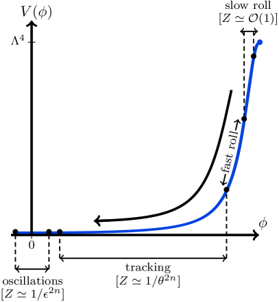
Figure 1: A schematic of the effective potential $V_{\text{eff}}(\phi)$ for the canonically normalized field $\phi$, associated with the wavefunction renormalization $Z(\theta)$ in Eq. (9). The non-trivial field dependence in $Z(\theta)$ induces deformations in the potential and alters the axion dynamics. The periods of evolution — slow roll, fast roll, tracking, and coherent oscillations — are labeled in their respective regions. The initial misalignment of the axion $\phi_{\text{in}}$ is assumed to be toward the edge of field space.

II.1.2 Tracking period

In the conventional axion dynamics [i.e., a model with $Z(\theta)=1$ for all $\theta$] the field would now transit into a harmonic region of the potential and undergo coherent oscillations. However, in our model, as the field enters $|\theta|\lesssim\mathcal{O}(1)$, the wavefunction changes form to $Z(\theta)\simeq 1/\theta^{2n}$. This change, and its associated deformation in $V_{\text{eff}}(\phi)$, dramatically alters the field trajectory and introduces a starkly different segment of evolution. In explicit terms, the canonical potential in this region is

$$V_{\text{eff}}(\phi)\simeq\frac{1}{2}\epsilon^{2}\Lambda^{4}\left\{\begin{array}[]{lcl}e^{2|\phi|/f-2}&\text{for}&n=1\\ \left[{n}-(n-1)\frac{\epsilon^{n-1}}{f}|\phi|\right]^{-\frac{2}{n-1}}&\text{for}&n>1\end{array}\right.\ .$$ (15)

The sort of dynamics induced by such a potential is well-known in the literature of quintessence models Wetterich (1988); Ratra and Peebles (1988). In particular, $V_{\text{eff}}(\phi)$ yields so-called “tracker” solutions: attractor-like field trajectories which have an identical late-time evolution for a wide range of initial conditions Zlatev et al. (1999); Steinhardt et al. (1999). These are characterized by an equation-of-state parameter (for axion pressure $P_{\phi}$ and energy density $\rho_{\phi}$)

$$w_{\phi}\equiv\frac{P_{\phi}}{\rho_{\phi}}=\frac{\frac{1}{2}\dot{\phi}^{2}-V_{\text{eff}}(\phi)}{\frac{1}{2}\dot{\phi}^{2}+V_{\text{eff}}(\phi)}$$ (16)

which converges to some fixed value, depending on parameters in the potential and the background cosmology. In Sec. A.1 we have provided a brief overview of the identification and classification of tracker solutions. Using that technology, we deduce that tracker solutions exist with $V_{\text{eff}}(\phi)$ for $n\geq 1$, which drive the axion equation-of-state parameter to

$$w_{\phi}=\frac{1+w-n}{n}$$ (17)

for background parameter $w$.

In other words, $n$ determines whether the axion energy density $\rho_{\phi}\propto a^{-3(1+w_{\phi})}$ dissipates less rapidly than the dominant component in the universe, which we assume is the radiation component ($w=\frac{1}{3}$). The case of an exponential potential ($n=1$) is unique, since it implies $w_{\phi}$ simply traces the background $w$ and the axion abundance $\Omega_{\phi}\equiv\rho_{\phi}/(3M_{P}^{2}H^{2})$ remains fixed. For potentials with larger $n$, the axion component behaves increasingly like vacuum energy, causing $\Omega_{\phi}$ to grow and eventually dominate if tracking lasts sufficiently long. Note that since we assumed $n$ is a positive integer, there is a bound $w_{\phi}\leq w$ and the axion energy density never dissipates more rapidly than the dominant component.

II.1.3 Coherently oscillating period

The tracking dynamics continues for as long as the angular field is confined to the $\epsilon\lesssim|\theta|\lesssim\mathcal{O}(1)$ region, i.e., for as long as the potential has the form in Eq. (15). However, as the field falls to $|\theta|\lesssim\epsilon$ it exits the tracking regime, and the wavefunction is frozen at a constant value $Z(\theta)\simeq 1/\epsilon^{2n}$. The potential is then approximately quadratic:

$$V_{\text{eff}}(\phi)\simeq\frac{1}{2}\frac{\epsilon^{2n}\Lambda^{4}}{f^{2}}\phi^{2}\quad\text{for}\quad|\phi|\lesssim\frac{f}{\epsilon^{n-1}}$$ (18)

and does not support a tracker solution.

To determine the field evolution during this final phase, we should compare the Hubble damping $H$ to the axion mass $m_{\phi}=\epsilon^{n}\Lambda^{2}/f$ at the time tracking completes. If we find that $3H\lesssim m_{\phi}$ the field will promptly begin to undergo coherent oscillations. On the other hand, if we find $3H\gtrsim m_{\phi}$, then it will sit in an overdamped phase until $H$ has dropped sufficiently for oscillations to commence. Assuming tracking lasts sufficiently long for the field to converge to the tracker trajectory, we can use Eq. (97), (99), and (17) to show that

$$\frac{3H}{m_{\phi}}\approx\sqrt{\frac{9n}{6n-4}}$$ (19)

at the time the field exits the tracking region. The ratio above is contained within $1.2\lesssim 3H/m_{\phi}\lesssim 2.1$, so the field commences coherent oscillations relatively soon after, regardless of $n$. Neglecting the minor $n$-dependence and any “overshooting” effect, the axion energy density at the time of oscillations is given approximately by

$$\rho_{\phi}\approx V_{\text{eff}}(\phi)\approx\frac{1}{2}\epsilon^{2}\Lambda^{4}\ .$$ (20)

Once coherent oscillations begin, the axion equation-of-state parameter averages to $\langle w_{\phi}\rangle\rightarrow 0$ and thus the axion behaves as matter. Ideally, the matter it constitutes would be abundant enough today to comprise the entirety of the DM. To calculate the relic abundance, we use that the temperature at which oscillations first occur is given approximately by $3H\approx m_{\phi}$:

$$T_{\text{osc}}^{4}\approx\frac{90M_{P}^{2}m_{\phi}^{2}}{g_{*}\pi^{2}}\ .$$ (21)

Then, employing conservation of entropy density, we find a relic abundance

$$\Omega_{\phi}h^{2}\approx\frac{\epsilon^{2(1-n)}}{g_{*}^{1/4}}\sqrt{\frac{m_{\phi}}{7\,\text{eV}}}\left(\frac{f}{10^{12}\,\text{GeV}}\right)^{2}$$ (22)

for a sufficiently long-lived axion.

It is important to note that for $n\neq 1$ a deformation in the potential enhances the relic abundance, while for $n=1$ it is independent of $\epsilon$. Moreover, $\Omega_{\phi}$ is independent of the initial misalignment angle $\theta_{\text{in}}$, as a result of the tracking dynamics encountered in the field evolution. This insensitivity reveals a significant departure from the traditional axion cosmology and also leads to a natural suppression of axionic isocurvature perturbations. We shall discuss the perturbations in more detail below and also provide a model-specific analysis in Sec. III.

Meanwhile, the lifetime of the axion is also enhanced if it decays primarily through an anomalous coupling to the electroweak sector. That is, the enhancement in $Z(\theta)$ near the origin generically implies a decay width $\Gamma_{\phi}\propto m_{\phi}^{3}/[f^{2}Z(0)]$ and thus an enhanced lifetime

$$\tau_{\phi}\approx\frac{6.6\times 10^{30}\,\text{s}}{\epsilon^{2n}}\left(\frac{f}{10^{12}\,\text{GeV}}\right)^{2}\left(\frac{7\,\text{eV}}{m_{\phi}}\right)^{3}\ ,$$ (23)

alleviating constraints from axion decays as the potential is deformed with $\epsilon\ll 1$.

II.2 Incorporating the baryogenesis mechanism

Let us now shift focus to embedding the mechanism for spontaneous baryogenesis in our model. We shall begin by describing the interactions necessary and discussing how they may appear in the UV theory. We then construct the Boltzmann equations for the matter-antimatter asymmetry and catalog the different ways in which production can occur.

II.2.1 Spontaneous $CPT$ violation

We must include interactions that spontaneously violate $CPT$ in the axion background, such as the effective coupling between the axion $\theta$ and the baryon current $J_{B}^{\mu}$:

$$\mathcal{L}_{\text{eff}}\supset\frac{1}{\mathcal{N}}\,\partial_{\mu}\theta\cdot J_{B}^{\mu}$$ (24)

where $\mathcal{N}$ is a constant that we clarify in what follows. The baryon current is given by

$$J^{\mu}_{B}=\frac{1}{3}\sum_{k}\left(q^{\dagger}_{k}\overline{\sigma}^{\mu}q_{k}+u^{*}_{k}\overline{\sigma}^{\mu}u_{k}+d^{*}_{k}\overline{\sigma}^{\mu}d_{k}\right)\ ,$$ (25)

where $q_{k}$, $u_{k}$, and $d_{k}$ are two-component Weyl spinors for the left-handed quark doublets, right-handed up-type quarks, and right-handed down-type quarks, respectively. Note also that we have suppressed $\text{SU}(3)_{c}$ and $\text{SU}(2)_{L}$ indices and the $\sigma^{\mu}$ are the Pauli matrices.

The homogeneity of the axion field in space implies its gradient is negligible and that Eq. (24) effectively reduces to an interaction

$$\mathcal{L}_{\text{eff}}\supset\frac{1}{\mathcal{N}}\,\partial_{0}\theta\cdot J_{B}^{0}\ .$$ (26)

Indeed, such a term spontaneously breaks $CPT$ symmetry once the field is set in motion, inducing an energy gap between baryons and antibaryons. If $B$-violating interactions are occurring in the thermal bath, then a baryon asymmetry is generated.

There are several ways to motivate the appearance of an interaction such as Eq. (24) in the effective Lagrangian. For instance, we may consider a spontaneous breaking of the baryon number symmetry $\text{U}(1)_{B}$ at high scales, in which $\theta$ is the corresponding Nambu-Goldstone boson (NGB), which in general would appear as the phase of some complex scalar field. In such a scenario, it is also necessary to specify the relationship between the axion potential and $\text{U}(1)_{B}$, as well as the effect of $B$-violating operators after integrating-out the radial scalar field.

However, other avenues exist through which we may generate such an interaction, even if $\theta$ is neutral under $\text{U}(1)_{B}$. By rotating the quark phases according to

$$q_{k} \longrightarrow e^{i\theta/\mathcal{N}}q_{k}$$

$$u_{k} \longrightarrow e^{i\theta/\mathcal{N}}u_{k}$$

$$d_{k} \longrightarrow e^{i\theta/\mathcal{N}}d_{k}\ ,$$ (27)

our term in Eq. (24) can be eliminated from the action, and we obtain an equivalent operator

$$\mathcal{L}_{\text{eff}}\supset\frac{3}{\mathcal{N}}\,\theta\left[\frac{\alpha_{2}}{16\pi}W^{\mu\nu}\widetilde{W}_{\mu\nu}-\frac{\alpha_{Y}}{8\pi}B^{\mu\nu}\widetilde{B}_{\mu\nu}\right]\ ,$$ (28)

with $W_{\mu\nu}$ the $\text{SU}(2)_{L}$ field strength, $B_{\mu\nu}$ the $\text{U}(1)_{Y}$ field strength, and $\widetilde{W}_{\mu\nu}$ and $\widetilde{B}_{\mu\nu}$ their respective duals. The factors $\alpha_{2}=g_{2}^{2}/(4\pi)$ and $\alpha_{Y}=g_{Y}^{2}/(4\pi)$ are the weak and hypercharge gauge coupling constants, respectively. Such an axion-like coupling of $\theta$ to the gauge bosons can naturally arise in the UV theory, independent of baryon number Witten (1984); Green and Schwarz (1984); Choi and Kim (1985a); Witten (1985); Choi and Kim (1985b); Svrcek and Witten (2006), if the normalization of the interaction is given by

$$\mathcal{N}=3/n\quad\text{for}\quad n=1,2,\cdots\ .$$ (29)

In what follows, we shall take $n=1$ for simplicity.

II.2.2 Source for $(B-L)$ violation

In addition to spontaneous $CPT$-violation, to satisfy the conditions for baryogenesis some $B$-violating interactions must also exist. The early-universe plasma is naturally equipped with such processes through weak sphaleron transitions. However, since the weak sphalerons preserve $(B-L)$ any baryon number generated through the spontaneous baryogenesis mechanism will still be annihilated once the axion settles to its minimum vacuum value. It is therefore essential that our theory also include interactions which break $(B-L)$. A well-motivated way to invoke such terms is through physics in the neutrino sector, where heavy right-handed neutrinos offer a natural explanation of neutrino masses and other associated phenomena. In the low-energy theory these appear in the form of a Weinberg operator

$$\mathcal{L}_{{L\hskip-4.26773pt/}}=\frac{(\ell_{i}\mathcal{H})(\ell_{j}\mathcal{H})}{2M_{*}}\ ,$$ (30)

where $\ell_{i}$ is an SM lepton doublet, $\mathcal{H}$ is the Higgs doublet, and neutrino observables determine the mass scale $M_{*}\simeq(10^{14}-10^{15})\,\text{GeV}$. Of course, the Weinberg operator breaks the lepton number $L$ in addition to $(B-L)$, so we shall denote associated processes by $L\hskip-4.26773pt/$. The existence of heavy right-handed neutrinos in the early universe may also lead to successful thermal leptogenesis through out-of-equilibrium decays Fukugita and Yanagida (1986). However, our study is dissociated from these models since $M_{*}$ is sufficiently heavy that the right-handed neutrinos are never produced in the thermal bath. The operator in Eq. (30) thus remains valid throughout our analysis.

II.2.3 Boltzmann evolution of asymmetry

Under the spontaneous breaking of $CPT$ by the term in Eq. (26), one may readily show that for sufficiently rapid $(B-L)$-violating processes, we obtain an equilibrium number-density asymmetry

$$n^{\text{eq}}_{B-L}=\frac{1}{6}\mu_{B-L}T^{2}\left[1+\mathcal{O}\left(\frac{\mu_{B-L}}{T}\right)^{2}\right]\ ,$$ (31)

where $\mu_{B-L}$ is the effective chemical potential associated with $(B-L)$. However, the asymmetry is not necessarily generated at equilibrium; rather, its evolution is more generally described by the Boltzmann equation

$$\dot{n}_{B-L}+3Hn_{B-L}=-\Gamma_{L\hskip-4.26773pt/}(n_{B-L}-n_{B-L}^{\text{eq}})\ .$$ (32)

A detailed derivation of the Boltzmann equation, in which we account for the role of sphaleron transitions in the plasma, is provided in Appendix B. Implementing these we can extract the interaction rate

$$\Gamma_{L\hskip-4.26773pt/}=\frac{9(171+65N_{f}-6N_{f}^{2})}{45+73N_{f}-3N_{f}^{2}}\cdot\frac{\gamma_{L\hskip-4.26773pt/}}{T^{3}}\ ,$$ (33)

in which

$$\gamma_{L\hskip-4.26773pt/}=\mathcal{O}(0.01)\frac{T^{6}}{M_{*}^{2}}$$ (34)

is the thermally averaged scattering rate density for processes sourced by the Weinberg operator in Eq. (30), and $N_{f}$ denotes the number of generations with Yukawa interactions in equilibrium during baryogenesis. The effective chemical potential is likewise given by

$$\mu_{B-L}=-g(N_{f})\cdot\partial_{0}\theta\ ,$$ (35)

for which the coefficient is derived in Eq. (128):

$$g(N_{f})=\frac{4}{3}\cdot\frac{36+65N_{f}-6N_{f}^{2}}{171+65N_{f}-6N_{f}^{2}}\ .$$ (36)

The weak sphaleron processes eventually decouple, and the final baryon number is set according to

$$n_{B}=\frac{28}{79}n_{B-L}\ .$$ (37)

The characteristic scale which determines the final $n_{B-L}$, however, is the temperature $T_{\text{D}}$ at which the processes derived from $\mathcal{L}_{L}\hskip-4.26773pt/$ decouple. In explicit terms, we define $T_{\text{D}}$ as the temperature at which the Hubble rate becomes dominant $H\geq\Gamma_{L\hskip-4.26773pt/}$. It is expressed as

$$T_{\text{D}}\simeq\mathcal{O}(\text{few})\sqrt{g_{*}}\,\frac{M_{*}^{2}}{M_{P}}\ ,$$ (38)

which in our study will be given by $T_{\text{D}}\approx 10^{13}\,\text{GeV}$. The conclusion we draw is that, given the assumptions above, a relatively high reheating temperature $T_{\text{RH}}\gtrsim T_{\text{D}}$ is necessary for processes sourced by Eq. (30) to ever achieve equilibrium. Indeed, depending on the temperature regime of the early radiation-dominated epoch, there are several different ways in which baryogenesis may unfold. To explore these in more detail, let us work instead with comoving quantities, such as the abundance $Y_{B-L}\equiv n_{B-L}/s$, in which

$$s=\frac{2\pi^{2}}{45}g_{*S}T^{3}$$ (39)

is the entropy density. It is then straightforward to determine the corresponding Boltzmann evolution

$$\frac{dY_{B-L}}{dT}=\frac{Y_{B-L}-Y_{B-L}^{\text{eq}}}{T_{\text{D}}}\ ,$$ (40)

where the equilibrium value $Y_{B-L}^{\text{eq}}\equiv n_{B-L}^{\text{eq}}/s$ is defined analogously to Eq. (31). An integral solution follows as

$$Y_{B-L}(T)=\int_{T}^{T_{\text{RH}}}dT^{\prime}\left[\frac{e^{-(T^{\prime}-T)/T_{\text{D}}}}{T_{\text{D}}}\right]Y_{B-L}^{\text{eq}}(T^{\prime})\ .$$ (41)

There are different limiting behaviors, depending on the relative size of the temperatures $T_{\text{D}}$ and $T_{\text{RH}}$, corresponding to equilibrium and out-of-equilibrium production. Below, we discuss each of these cases.

II.2.4 Equilibrium production

In the $T_{\text{D}}\ll T_{\text{RH}}$ regime, the function enclosed within square brackets of Eq. (41) approaches a Dirac delta function $\delta(T^{\prime}-T)$, which holds for temperatures $T>T_{\text{D}}$. The asymmetry closely follows its equilibrium value $Y_{B-L}(T)\simeq Y_{B-L}^{\text{eq}}(T)$ in that regime and reproduces the result in Eq. (31). However, once the plasma cools below $T<T_{\text{D}}$, equilibrium productions ceases and the asymmetry “freezes out.” Therefore, we obtain a late-time asymmetry

$$Y_{B-L}\simeq Y_{B-L}^{\text{eq}}(T_{\text{D}})\ .$$ (42)

The interplay between the equilibrium production of $Y_{B-L}$ and the axion dynamics is significant in determining the final baryon asymmetry. In particular, the late-time yield can be ruined if decoupling does not occur until after the axion undergoes oscillations — in this event $\mu_{B-L}$ oscillates as well, and the asymmetry is washed out. Almost as severely, if decoupling occurs within the tracking period, the field velocity and thus $Y_{B-L}$ is considerably weakened. In the context of equilibrium production we shall then assume that

$$\frac{\Lambda^{2}}{f}\ll\sqrt{5}H(T_{\text{D}})\approx 3T_{\text{D}}^{2}/M_{P}\ ,$$ (43)

which implies the field is slowly rolling at decoupling. The yield is then determined by the slow-roll trajectory in Eq. (12) and we find an approximate expression

$$Y_{B-L}\sim 10^{-3}\frac{1}{\epsilon^{2n}}\frac{m_{\phi}^{2}M_{P}}{T_{\text{D}}^{3}}\ .$$ (44)

Note that taking $\epsilon$ to smaller values, and thereby deforming the potential more acutely, corresponds to an enhancement in the matter-antimatter asymmetry.

II.2.5 Out-of-equilibrium production

Let us now consider the opposite temperature regime, in which reheating occurs below the scale of decoupling $T_{\text{RH}}<T_{\text{D}}$. In such a scenario, processes which violate $(B-L)$ are always out-of-equilibrium, i.e., $Y_{B-L}<Y_{B-L}^{\text{eq}}$ for all temperatures. Consequently, the asymmetry production occurs in a different fashion, weakly but persistently driven by the $Y_{B-L}^{\text{eq}}/T_{\text{D}}$ term in Eq. (40). The production mechanism here is analogous to the “freeze-in” production in the DM literature Hall et al. (2010). It is straightforward to obtain the yield

$$Y_{B-L}\simeq\frac{32}{25\pi^{2}g_{*}}\frac{\Lambda^{2}}{fT_{\text{D}}}\mathcal{I}(\theta_{\text{in}})\ ,$$ (45)

in which the integral $\mathcal{I}(\theta)$ is defined by

$$\mathcal{I}(\theta)\equiv\int_{0}^{\infty}du\,\frac{1}{u}\frac{d\theta}{du}\ ,$$ (46)

for a dimensionless temporal parameter $u\equiv\Lambda^{2}t/f$. It can be shown using Eq. (4) that $\mathcal{I}(\theta_{\text{in}})$ gives only an $\mathcal{O}(1)$ contribution. Finally, assuming baryogenesis occurs at temperatures $T\gtrsim 100\,\text{GeV}$, we conclude that

$$Y_{B-L}\sim 10^{-3}\frac{\Lambda^{2}}{fT_{\text{D}}}=10^{-3}\frac{1}{\epsilon^{n}}\frac{m_{\phi}}{T_{\text{D}}}$$ (47)

within order-of-magnitude accuracy.

We observe for both the equilibrium production in Eq. (42) and the out-of-equilibrium production above, for a fixed axion mass the asymmetry is enhanced by deformations $\epsilon\ll 1$ in the potential. Thus, possibilities for model-building can exist in either of these two regimes.

On another note, by comparing the scaling behavior for the axion relic abundance $\Omega_{\phi}\propto\epsilon^{2(1-n)}$ [see Eq. (22)] to the estimates for the late-time asymmetry $Y_{B-L}$ above, we find that $n=1$ has some intriguing properties. In particular, while the baryon asymmetry is always enhanced by $\epsilon\ll 1$, the relic abundance is unaffected for $n=1$, providing us with some modularity between these two cosmological quantities. We shall investigate these details further in the context of the explicit model constructed in Sec. III, which is specific to the $n=1$ case.

II.3 Isocurvature perturbations

As alluded to above, for successful baryogenesis the axion must be relatively light $\Lambda^{2}/f\ll H_{I}$ during inflation, for an inflationary Hubble scale $H_{I}$. Therefore, it is subject to quantum fluctuations with amplitude

$$\delta\phi_{\text{in}}=\frac{H_{I}}{2\pi}\ ,$$ (48)

in the pure-de Sitter limit. As a result, we find corresponding fluctuations in the angular field

$$\delta\theta_{\text{in}}=\frac{1}{\sqrt{Z(\theta_{\text{in}})}}\frac{H_{I}}{2\pi f}\ .$$ (49)

The sources of primordial scalar perturbations are decomposed into linearly independent adiabatic and isocurvature modes, i.e., perturbations to the total energy density and the local equation of state, respectively. The fluctuations $\delta\theta_{\text{in}}$ source only the isocurvature mode, which is subdominant and tightly constrained by observations of the CMB Akrami et al. (2018). Furthermore, since the baryon asymmetry is generated via the effective chemical potential $\mu_{B-L}\sim\partial_{0}\theta$, baryonic isocurvature perturbations $\delta Y_{B}$ also exist and play an important role.

As illustrated in Sec. II.1, the presence of a tracking region in the canonical potential $V_{\text{eff}}(\phi)$ renders the late-time axion dynamics insensitive to the initial field displacement. Consequently, the axionic isocurvature perturbations are generically suppressed with a magnitude corresponding to the duration of the tracking period. In the remainder of this section, we shall assume tracking lasts for a sufficiently long period that we may focus exclusively on the baryonic component.

As discussed above, $Y_{B}$ may be populated while driving the system either at equilibrium (freeze-out) or out-of-equilibrium (freeze-in). In the former case, the baryon asymmetry produced is simply $Y_{B}\approx Y_{B}^{\rm eq}\propto\mu_{B-L}$ evaluated at the decoupling temperature $T_{\text{D}}$. Therefore, the baryonic perturbation is

$$\frac{\delta Y_{B}}{Y_{B}}\simeq\frac{\delta\mu_{B-L}}{\mu_{B-L}} =\left.\frac{d\log\mu_{B-L}^{\rm eq}}{d\theta}\frac{1}{\sqrt{Z(\theta)}}\frac{H_{I}}{2\pi f}\right|_{\theta_{\text{in}}}$$

$$=\left.\frac{d\log\dot{\theta}}{d\theta}\frac{1}{\sqrt{Z(\theta)}}\frac{H_{I}}{2\pi f}\right|_{\theta_{\text{in}}}\ ,$$ (50)

also evaluated at $T_{\text{D}}$. As before, we assume decoupling occurs during the slow-roll period, so the trajectory is given by Eq. (12):

$$\dot{\theta}\simeq-\frac{1}{5H}\frac{\Lambda^{4}}{f^{2}}\frac{1}{Z(\theta)}\frac{dU}{d\theta}\ ,$$ (51)

which we have written in the non-canonical basis. Assuming the field moves negligibly from its initial misalignment $\theta\simeq\theta_{\text{in}}$, the approximate isocurvature is

$$\mathcal{P}_{\mathcal{S}\mathcal{S}}\simeq\frac{1}{Z(\theta)}\!\left(\!\frac{\Omega_{B}}{\Omega_{\text{CDM}}}\frac{H_{I}}{2\pi f}\!\right)^{\!2}\!\left.\left[\frac{U^{\prime\prime}(\theta)}{U(\theta)}-\frac{Z^{\prime}(\theta)}{Z(\theta)}\right]^{\!2}\right|_{\theta_{\text{in}}}\!$$ (52)

where a prime denotes a derivative with respect to the field $\theta$. Interestingly, the two terms in Eq. (52) may have opposite signs, allowing for cancellations and a vanishing perturbation. Additionally, the first term can clearly vanish if $\theta_{\text{in}}$ sits at any of its inflection points.

On the other hand, in the case of out-of-equilibrium production, we can derive the baryonic perturbation directly from Eq. (45):

$$\frac{\delta Y_{B}}{Y_{B}}\simeq\left.\frac{d\log\mathcal{I}(\theta)}{d\theta}\frac{1}{\sqrt{Z(\theta)}}\frac{H_{I}}{2\pi f}\right|_{\theta_{\text{in}}},$$ (53)

which results in the expression for the power

$$P_{\mathcal{S}\mathcal{S}}\simeq\left.\frac{1}{Z(\theta)}\left(\!\frac{\Omega_{B}}{\Omega_{\text{CDM}}}\frac{H_{I}}{2\pi f}\!\right)^{\!2}\left(\frac{d\log\mathcal{I}(\theta)}{d\theta}\right)^{\!2}\right|_{\theta_{\text{in}}}.\\$$ (54)

The integral $\mathcal{I}(\theta_{\text{in}})$ is over time [see Eq. (46)] and therefore it is not a simple function of the potential or its derivatives. Instead, these results must be obtained numerically from the equation of motion.

The power spectra in Eq. (52) and Eq. (54) act as constraints on the parameter space given an explicit model realization. In the remainder of this paper, we shall consider such a concrete model, and show a more detailed study of its phenomenology and cosmological constraints, using numerical simulations where necessary.

III An explicit model: The continuum-clockwork axion

In Sec. II, we described a general construction by which an axion-like field $\theta$ may dynamically generate matter-antimatter asymmetry in the early universe, while also serving as a plausible DM candidate. The crux of this approach is the appearance of a field-dependent wavefunction renormalization $Z(\theta)$ that meets some basic requirements. In particular, if the wavefunction is enhanced $Z\gg 1$ near the minimum of the axion potential, but remains $Z=\mathcal{O}(1)$ elsewhere, then the potential $V_{\text{eff}}(\phi)$ for the canonically normalized field $\phi$ is “deformed” in a way that suppresses its mass, generically suppresses its couplings, and can dramatically alter its dynamics.

In this section, we demonstrate that models exist with the ingredients necessary to furnish such a wavefunction renormalization. As an explicit example, we focus on “continuum-clockwork” (CCW) Giudice and McCullough (2017a); Craig et al. (2017); Giudice and McCullough (2017b); Choi et al. (2017) axion models, incorporating the interactions necessary for spontaneous baryogenesis along the lines of Sec. II.2. We show that regions of parameter space exist in which both the observed baryon asymmetry and dark matter abundance are produced. Furthermore, we show that other phenomenological constraints, such as those from decays and isocurvature perturbations, are adequately contained.

III.1 Overall features and construction

The hallmark of the “clockwork mechanism” Kim et al. (2005); Choi et al. (2014); Choi and Im (2016); Kaplan and Rattazzi (2016) is the generation of an exponential hierarchy of couplings in theories with exclusively $\mathcal{O}(1)$ input parameters. There have been many studies and implementations, including on the QCD axion Higaki et al. (2016a, b, c); Farina et al. (2017); Coy et al. (2017); Long (2018), dark matter Hambye et al. (2017); Kim and McDonald (2018); Kim and Mcdonald (2018); Goudelis et al. (2018), cosmological topics Fonseca et al. (2016); Saraswat (2017); Kehagias and Riotto (2017); Park and Shin (2018a); Agrawal et al. (2018), flavor physics Hong et al. (2018); Park and Shin (2018b); Ibarra et al. (2018); Alonso et al. (2018), and generalizations or more formal aspects Giudice and McCullough (2017a); Craig et al. (2017); Giudice and McCullough (2017b); Choi et al. (2017); Ahmed and Dillon (2017); Ben-Dayan (2017); Lee (2018); Giudice et al. (2018); Choi et al. (2017); Teresi (2018).

To introduce this idea more explicitly, let us consider a model with $N+1$ scalars $\chi_{i}$. The clockwork mechanism typically arises through “nearest-neighbor” interactions between adjacent scalars, such as through terms proportional to $(\chi_{i+1}-q\chi_{i})^{2}$, where $q>1$ is a dimensionless parameter. Then, the lightest mass eigenstate $\phi$ in the system exhibits most of the interesting phenomenology. In particular, if the $\chi_{i}$ have couplings $Q_{i}$ to some other sector, then these contribute to the coupling for $\phi$ as

$$Q_{\phi}~{}\propto~{}\sum_{i=0}^{N}\frac{Q_{i}}{q^{N-i}}\ .$$ (55)

That is, the coupling for the lightest state is determined through a non-uniform distribution over the $Q_{i}$. As their contributions are weighted by powers $1/q^{N-i}$, the distribution is effectively “localized” toward $Q_{N}$, where the parameter $q$ sets the strength of the localization.

A natural extension of this idea is to construct the clockwork mechanism in the continuum limit $N\rightarrow\infty$, where the theory is reinterpreted as that of a discretized compact extra dimension. In the continuum, the nearest-neighbor interactions composed of $\chi_{i+1}-q\chi_{i}$ are mapped onto $\partial_{y}\chi(x,y)-m\chi(x,y)$, where $m>0$, the extra spatial coordinate is $y$, and $\chi(x,y)$ is now a five-dimensional scalar field. This type of combination can be realized by bulk and boundary mass terms. Moreover, several of the phenomena found in the discrete clockwork theory are mapped onto the extra-dimensional theory in some way. In particular, the profile for the zero-mode is exponentially localized toward a boundary in the extra dimension, analogous to the localization of the coupling in Eq. (55). Similar phenomenological implications arise from this as well, such as the suppression of couplings to other boundary operators.

Furthermore, interesting observations can be made if the CCW theory is constructed from a five-dimensional angular field $\theta(x,y)$. Due to the periodicity $\theta\rightarrow\theta+2\pi$, the clockwork interactions should have the general form $\partial_{y}\theta(x,y)-mV(\theta)$, for periodic $V(\theta)=V(\theta+2\pi)$. As discussed in Ref. Choi et al. (2017), this results in a more non-trivial localization of the lightest mode along the extra dimension, which has subtle implications for the axion couplings and its dynamics. While the specific details are beyond the scope of this paper, it provides us the essential features by which we shall realize a field-dependent wavefunction renormalization of the form proposed in Sec. II.

Let us therefore begin by considering the action for this particular five-dimensional realization:

$$\mathcal{S}_{\theta}=\frac{f_{5}^{3}}{2}\int d^{4}xdy\left[(\partial_{\mu}\theta)^{2}-\left(\partial_{y}\theta-m\sin\theta\right)^{2}\right]\ ,$$ (56)

where we compactify over an $\mathcal{S}_{1}/\mathbb{Z}_{2}$ orbifold of radius $R$, and $m$ sets the scale for bulk and boundary terms. The SM fields are assumed to be confined to the $y=0$ brane and flat space is assumed for tractability. Note that a massless four-dimensional mode $\phi(x)$ is found in the spectrum:

$$\tan\left[\frac{\theta(x,y)}{2}\right]=e^{my}u\!\left[\phi(x)\right]\ ,$$ (57)

where the function $u[\phi]$ enforces canonical normalization for $\phi$ over its domain. Namely, we define

$$u\!\left[\phi\right]\equiv e^{-\pi mR}\text{sc}\bigg{[}\frac{\phi}{2f}\bigg{|}1-e^{-2\pi mR}\bigg{]}$$ (58)

in which $f^{2}\equiv f_{5}^{3}(1-e^{-2\pi mR})/(2m)$ and $\text{sc}[\,\cdot\,|\,\cdot\,]$ is a Jacobi elliptic function. Integrating out the higher KK modes and the compact dimension, we construct the low-energy effective action

$$S_{\theta}\approx\frac{1}{2}\int d^{4}x\,\frac{f_{5}^{3}}{m}\frac{\left(\partial_{\mu}\theta\right)^{2}}{\coth\left(\pi mR\right)-\cos\theta}\ ,$$ (59)

where it is understood that $\theta\equiv\theta(x,0)$ is evaluated at the $y=0$ brane. The wavefunction renormalization as defined in Eq. (3) is easily extracted:

$$Z(\theta)\simeq\frac{1}{\coth\left(\pi mR\right)-\cos\theta}\ .$$ (60)

In the regime $mR\gtrsim\mathcal{O}(\text{few})$ that clockwork has a substantial effect, this reduces to

$$Z(\theta)\simeq\frac{2}{1+2\epsilon^{2}-\cos\theta}\ ,$$ (61)

where $\epsilon\equiv e^{-\pi mR}$ is a small parameter. It is manifest that $Z(\theta)\simeq\mathcal{O}(1)$ near the boundaries of field space and $Z(\theta)\gg 1$ near the origin. Furthermore, expanding about the origin we find $Z(\theta)\approx 4/\theta^{2}$, which is the necessary scaling to ensure the desired “tracking” dynamics. It is then evident that the CCW axion reproduces the $n=1$ form of Eq. (9) and we can conclude: CCW axions satisfy our minimal requirements for spontaneous baryogenesis driven by a stable axion DM candidate.

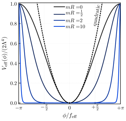
Figure 2: The effective 4D canonical potential $V_{\text{eff}}(\phi)$ that arises for a continuum-clockwork axion, where the different curves show various choices for the clockwork parameter $mR$, and the horizontal axis is normalized such that curves are plotted over the full field range $\phi\in\left[-\pi f_{\text{eff}},+\pi f_{\text{eff}}\right]$.

Having satisfied the minimal set of conditions from Sec. II, let us further investigate the details of this model. While the symmetry of the action in Eq. (56) yields a massless zero-mode $\phi$, any small deviation in boundary masses will generate an effective four-dimensional potential $\Lambda^{4}(1-\cos\theta)$, which in the canonical basis reads

$$V_{\text{eff}}(\phi)=\frac{2\Lambda^{4}}{\displaystyle{1+\frac{1}{u^{2}\!\left[\phi\right]}}}\ .$$ (62)

While $V_{\text{eff}}(\phi)$ is periodic in $\phi$, it is important to note the period is not given by $2\pi f$, but rather by the expression

$$2\pi f_{\text{eff}} \equiv 4fK\left(1-\epsilon^{2}\right)$$

$$\xrightarrow[~{}\epsilon^{2}\ll 1~{}]{}2f\log\left(\frac{16}{\epsilon^{2}}\right)\ ,$$ (63)

where $K(\cdot)$ is the complete elliptic integral of the first kind. As a result, the field range of the canonical four-dimensional axion is effectively extended for finite $mR$.

In Fig. 2 the potential is shown for several values of $mR$, normalized so that the curves all span the same domain. As soon as we exceed $mR\gtrsim\mathcal{O}(\text{few})$ the potential quickly shows substantial deformations, with the minimum flattened along most of the field range. The resulting axion mass

$$m_{\phi}^{2}\equiv\!\left.\frac{\partial^{2}V_{\text{eff}}}{\partial\phi^{2}}\right|_{\phi=0}\!\!\!\!=~{}e^{-2\pi mR}\frac{\Lambda^{4}}{f^{2}}\ ,$$ (64)

is exponentially suppressed relative to the standard $mR=0$ sinusoidal potential. Indeed, the suppression of this mass scale confirms the CCW axion model is equipped with one of the imperative features.

The other feature necessary to avoid phenomenological complications is the suppression of axion decays to SM states. In the discrete clockwork theory described above Eq. (55), this suppression would arise for the light state $\phi$ if the SM were coupled to the endpoint $\chi_{N}$ opposite to where $\phi$ is localized. Analogously, in the continuum limit this corresponds to SM fields confined to the $y=0$ brane. In other words, if we have an interaction between the axion and some generic SM operator $\mathcal{O}(x)$

$$\mathcal{S}_{\theta}\supset\int d^{4}x\theta(x,0)\mathcal{O}(x)\ ,$$ (65)

we can write it in the canonical basis using

$$\phi=f\int\!\!\sqrt{Z(\theta)}d\theta~{}\approx~{}\frac{\pi f_{\text{eff}}}{\epsilon}\frac{F\big{(}\frac{\theta}{2}\big{|}\!-\frac{1}{\epsilon^{2}}\big{)}}{K(1-\epsilon^{2})}\ ,$$ (66)

where $F(\cdot\,|\,\cdot)$ is the incomplete elliptic integral of the first kind. Let us examine how the coupling is affected for larger $mR$. Away from the minimum of the potential $\phi\approx\pi f_{\text{eff}}$ is quickly approached and thus the coupling is not significantly affected beyond the minor enhancement of $f_{\text{eff}}$. However, around the minimum Eq. (66) reduces to $\theta\approx\epsilon\phi/f$, so that couplings to $\phi$ are exponentially suppressed. For example, if we take the operator $\mathcal{O}(x)\sim F_{\mu\nu}\widetilde{F}^{\mu\nu}$, for some SM field strength $F_{\mu\nu}$ and its dual $\widetilde{F}_{\mu\nu}$, then the axion decay rate suffers a suppression

$$\Gamma_{\phi}\propto\frac{1}{Z(0)}\frac{m_{\phi}^{3}}{f^{2}}=\epsilon^{2}\cdot\frac{m_{\phi}^{3}}{f^{2}}\ .$$ (67)

Note that this suppression acts in addition to that implicitly included in the mass [see Eq. (64)].

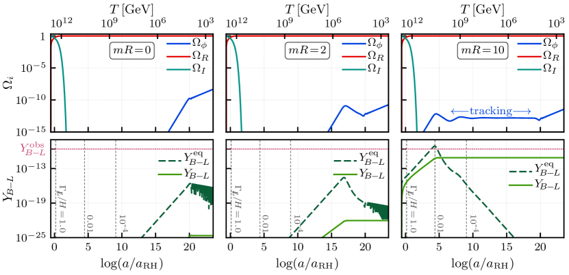
Figure 3: A numerical simulation of the dynamics in the explicit realization of our scheme, using a continuum-clockwork axion. In each column, a different clockwork strength $mR\in[0,2,10]$ is used. The rows show the evolution of cosmological abundances $\Omega_{i}=\{\Omega_{I},\Omega_{R},\Omega_{\phi}\}$ and $Y_{B-L}\equiv n_{B-L}/s$, as a function of the number of e-folds since reheating $\log(a/a_{\text{RH}})$, respectively. The axion mass $m_{\phi}=1\,\text{eV}$, initial misalignment $\theta_{\text{in}}=3\pi/4$, and scales for inflation $H_{I}=\Gamma_{I}=10^{8}\,\text{GeV}$ are fixed. The equilibrium $Y_{B-L}^{\rm eq}$ curves indicate that spontaneous baryogenesis proceeds out-of-equilibrium in this model, as also indicated by the $\Gamma_{L\hskip-4.26773pt/}/H$ values marked by vertical gray-dashed lines. As $mR$ is increased, despite the mass being fixed, production of asymmetry is exponentially more efficient. In the right-hand panel the “tracking” behavior of Sec. II.1.2 appears for the axion, during which the field does not oscillate, but follows a radiation-like equation of state $w_{\phi}\approx 1/3$, matching that of the background.

III.2 Early dynamics and baryogenesis

Above we have constructed the axion sector of the theory, however, we must also incorporate the necessary ingredients for baryogenesis. We shall proceed in a manner parallel with Sec. II.2, specializing our analysis to the continuum-clockwork model. As we argued previously, the motion of the axion $\partial_{0}\phi\neq 0$ spontaneously breaks $CPT$ symmetry if it couples derivatively to a baryon current, as in Eq. (24). In addition, the Weinberg operator in Eq. (30) provides a source for processes that violate $(B-L)$. Assuming a similar interaction in this model, the effective chemical potential from Eq. (35) in the canonical basis takes the form

$$\mu_{B-L}(\phi,\dot{\phi})=-g(N_{f})\cdot\frac{\frac{1}{2\Lambda^{4}}\left|\frac{\partial V_{\text{eff}}}{\partial\phi}\right|\dot{\phi}}{\sqrt{\left(1-\frac{V_{\text{eff}}}{2\Lambda^{4}}\right)\frac{V_{\text{eff}}}{2\Lambda^{4}}}}\ ,$$ (68)

where $V_{\text{eff}}(\phi)$ was used for a more succinct expression.

In order to numerically simulate the early dynamics we make several assumptions. Let us suppose a period of inflation with Hubble parameter $H_{I}$ during which the axion is misaligned from the minimum of its potential by angle $\theta_{\text{in}}\in[-\pi,\pi]$. Then, the reheating epoch is modeled by assuming the energy density in the inflaton $\rho_{I}\approx 3M_{P}^{2}H_{I}^{2}$ decays into radiation $\rho_{R}$ at some rate $\Gamma_{I}$. It follows that these quantities evolve as

$$\dot{\rho}_{I}+3H\rho_{I} =-\Gamma_{I}\rho_{I}$$

$$\dot{\rho}_{R}+4H\rho_{R} =+\Gamma_{I}\rho_{I}+\Gamma_{\phi}\rho_{\phi}\ ,$$ (69)

where the Hubble parameter is given by

$$H^{2}=\frac{\rho_{I}+\rho_{R}+\rho_{\phi}}{3M_{P}^{2}}\ ,$$ (70)

and

$$\rho_{\phi}=\frac{1}{2}\dot{\phi}^{2}+V_{\text{eff}}(\phi)$$ (71)

is the energy density in the axion field. Meanwhile, the axion equation of motion reads

$$\ddot{\phi}+\left(3H+\Gamma_{\phi}\right)\dot{\phi}+\frac{\partial V_{\text{eff}}}{\partial\phi}=\frac{\partial\mu_{B-L}}{\partial\dot{\phi}}\Gamma_{L\hskip-4.26773pt/}\left(n_{B-L}-n_{B-L}^{\text{eq}}\right)\ .$$ (72)

The term on the right-hand side is due to backreaction from $(B-L)$ generation and is usually negligible. As the axion is set into motion it drives the production of $Y_{B-L}$, which follows the Boltzmann evolution in Eq. (40).

In Fig. 3 the evolution of two types of quantities — the cosmological abundances $\Omega_{i}\equiv\rho_{i}/(3M_{P}^{2}H^{2})$ and abundance $Y_{B-L}$ — are shown in the two rows of panels, as functions of the number of e-folds since reheating $\log(a/a_{\text{RH}})$. Almost all parameters are held fixed: the mass $m_{\phi}=1~{}\text{eV}$, effective scale $f_{\text{eff}}=10^{13}\,\text{GeV}$, and misalignment angle $\theta_{\text{in}}=3\pi/4$. However, we have varied the strength of the clockwork mechanism $mR=\{0,2,10\}$ in each column. Therefore, the left-hand column shows dynamics for the traditional sinusoidal axion potential, the right-hand column shows a substantially deformed potential, and the center column shows an intermediate case between these two regimes.

Note that results are sensitive to inflationary scales $\Gamma_{I}$ or $H_{I}$ only if they are exceeded by the initial scale of curvature $\sqrt{\left|V_{\text{eff}}^{\prime\prime}(\phi_{\text{in}})\right|}\approx m_{\phi}e^{\pi mR}$. The curvature exceeding $H_{I}$ implies the axion is a heavy field during inflation and we shall exclude this region. On the other hand, if the curvature exceeds $\Gamma_{I}$ it implies the axion is set in motion prior to reheating. Then, washout effects that suppress the asymmetry can become sizeable. In this section, we look to identify phenomenologically viable regions of parameter space, and thus as a simplifying assumption we take these scales to be comparable $\Gamma_{I}\sim H_{I}$.

The influence from the variation of $mR$ in Fig. 3 is seen most immediately in the plots of $Y_{B-L}$. The deformation of the potential sets the axion in motion at higher temperatures. Nevertheless, we always find $\Gamma_{L\hskip-4.26773pt/}/H\lesssim 1$ such that $Y_{B-L}$ never exactly tracks the equilibrium value $Y_{B-L}^{\rm eq}$, i.e., this model exhibits the “freeze-in” spontaneous baryogenesis discussed in Sec. II, in contrast to more common examples in the literature. As a result, the asymmetry is mostly set during the fast-roll period and remains frozen at that value. Using the estimate in Eq. (47) and evaluating at the fast-roll temperature $T_{\text{FR}}$ from Eq. (14) we find

$$\frac{Y_{B-L}}{Y_{B-L}^{\text{eq}}}\approx\frac{1}{3}\sqrt{\frac{1}{5}\frac{m_{\phi}M_{P}}{T_{\text{D}}^{2}}}e^{\pi mR/2}\ ,$$ (73)

when production ceases. The above expression demonstrates how the deformation of the potential through the clockwork mechanism (i.e., the exponential factor $e^{\pi mR/2}$) enables sufficient baryogenesis while maintaining a relatively light axion.

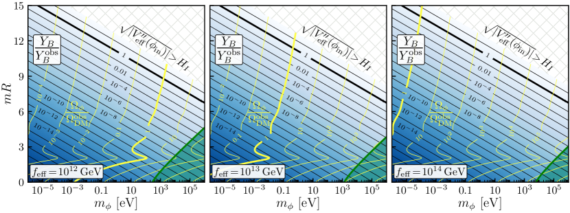
Figure 4: The result of numerical simulations, showing the normalized baryon abundance $Y_{B}/Y^{\text{obs}}_{B}$ (black contours, blue shading) and axion relic abundance $\Omega_{\phi}/\Omega_{\text{DM}}^{\text{obs}}$ (yellow contours), plotted with respect to the axion mass $m_{\phi}$ and clockwork parameter $mR$. The two thick curves mark where the observed values are attained. The scale $f_{\text{eff}}$ is fixed to a different value in each panel, while the other parameters are held fixed to values used in previous figures: $H_{I}=10^{8}\,\text{GeV}$ and $\theta_{\text{in}}=3\pi/4$. The hatched region rules axion oscillations during inflation, while the green region shows where the axion is too unstable to decays ($\tau_{\phi}\lesssim 10^{26}\,\text{seconds}$) to serve as a DM candidate. Other relevant constraints come from isocurvature perturbations, which we cover in Sec. III.4.

Another interesting dynamical feature is found in the $mR=12$ column of Fig. 3. Although the deformation of $V_{\text{eff}}(\phi)$ sets the axion in motion earlier, it does not undergo coherent oscillations until much later when $3H\lesssim m_{\phi}$. Instead, during this period the trajectory is such that $\Omega_{\phi}$ is temporarily fixed, with a radiation-like equation of state $w_{\phi}\approx 1/3$. Indeed, we have identified the “tracking” phenomenon, which we have discussed in more generality in Sec. II.1.2. We expect this dynamics to occur over the field range where $Z(\theta)\sim 1/\theta^{2}\sim e^{\left|\phi\right|/f}$, and taking $mR\gtrsim\mathcal{O}(\text{few})$ is sufficient to generate such a region. We find that

$$V_{\text{eff}}(\phi)\approx\frac{1}{2}m_{\phi}^{2}f^{2}e^{\left|\phi\right|/f}$$ (74)

is a good approximation over $f\lesssim|\phi|\lesssim(\log 2+2\pi mR)f$. The enhancement of the axion field range by $f_{\text{eff}}/f\approx 1+2mR$ makes such a displacement easy to achieve. The trajectory of the tracker is found using that

$$\frac{1+w_{\phi}}{1-w_{\phi}}=\frac{\frac{1}{2}\dot{\phi}^{2}}{V_{\text{eff}}(\phi)}$$ (75)

is approximately constant. The resulting solution

$$\left|\phi(t)\right|\approx-2f\log\left[e^{-\frac{\left|\phi_{\rm tr}\right|}{2f}}+\frac{m_{\phi}\left(t-t_{\rm tr}\right)}{\sqrt{2}}\right]\ ,$$ (76)

naturally depends weakly on the initial field amplitude $\phi_{\rm tr}\equiv\phi(t_{\rm tr})$ as it enters the tracking epoch. Considering that tracking ends once $m_{\phi}t\sim\mathcal{O}(1)$, the dependence on $\phi_{\rm tr}$ is ultimately washed away if $\phi_{\rm tr}\gtrsim f_{\text{eff}}$. Therefore, for sufficiently deformed potentials the late-time axion field is insensitive to the initial misalignment angle $\theta_{\text{in}}$, in contrast to the standard $mR=0$ case.

III.3 Survey of viable regions

We are now in position to discuss the phenomenological viability of this explicit model. As a first requirement we must verify the existence of regions in parameter space which have both the observed dark matter abundance $\Omega_{\text{DM}}^{\text{obs}}\approx 0.26$ and baryon abundance $Y_{B}^{\text{obs}}\approx 8.6\times 10^{-11}$. Furthermore, regions in which the axion is not sufficiently stable, i.e., lifetimes longer than $\tau_{\phi}\gtrsim 10^{26}\,\sec$ Chen and Kamionkowski (2004); Zhang et al. (2007), must be excluded. Indeed, regions with substantial deformations, i.e., at least moderately large $mR$, are where we expect to find viability in these respects.

As we have found above, such a regime is also associated with a tracking period for the axion. While tracking has little direct effect on the development of baryon asymmetry, it does have an marked influence on the relic abundance $\Omega_{\phi}$. Namely, employing the tracking-field solution in Eq. (76) we find at the onset of coherent oscillations $\rho_{\phi}\approx m_{\phi}^{2}f^{2}$, so that at present day

$$\Omega_{\phi}h^{2}\approx 0.12\left(\frac{f_{\text{eff}}}{10^{13}\,\text{GeV}}\cdot\frac{12}{mR}\right)^{2}\sqrt{\frac{m_{\phi}}{0.53~{}\text{eV}}}\ ,$$ (77)

In the region of interest $mR\gtrsim\mathcal{O}(\text{few})$ we find agreement with numerical computations to $\lesssim 10\%$. Note that the insensitivity of $\Omega_{\phi}$ to the initial misalignment angle $\theta_{\text{in}}$ is a result of the attractor-like dynamics and distinguishes our result from the standard axion cosmology.

An analytical approximation for the baryon asymmetry can also be constructed using the general result in Eq. (47), taking the integrated $\mathcal{O}(1)$ factor to be unity. We find an approximate expression

$$Y_{B}\sim 10^{-10}\left(\frac{m_{\phi}}{0.53~{}\text{eV}}\right)e^{\pi(mR-12)}\ ,$$ (78)

which holds to at least order-of-magnitude accuracy throughout the parameter space.

The results of our numerical simulations span the $\{m_{\phi},mR,f_{\text{eff}}\}$ space and are shown in Fig. 4. In each panel, contours show both the normalized baryon abundance $Y_{B}/Y_{B}^{\text{obs}}$ (black) and axion abundance $\Omega_{\phi}/\Omega_{\text{DM}}^{\text{obs}}$ (yellow). The sole distinction between each panel is the choice for the scale $f_{\text{eff}}$. The green regions show exclusions due to axion decays. As expected from Eq. (67), for even moderately large $mR$ these regions are substantially reduced in size. The points of intersection between the two thickest curves correspond to viable configurations that match observations, and these plots show that viable regions exist over all the panels shown in Fig. 4. The only constraints not yet applied are bounds on isocurvature perturbations, which is the focus for the remainder of the section.

III.4 Isocurvature perturbations

In the more general analysis provided in Sec. II.3, several significant observations were made regarding the axionic and baryonic isocurvature perturbations. Moreover, power spectra for these perturbations were found for both in-equilibrium and out-of-equilibrium production of the baryon asymmetry. We conclude this section with a more thorough treatment, in which the perturbation equations are solved numerically, within the context of the continuum-clockwork axion model.

III.4.1 System of perturbations

In our analysis, for perturbations of the FRW background, we use the conformal Newtonian gauge, defined by the line element Bardeen (1980); Mukhanov et al. (1992):

$$ds^{2}=(1+2\Phi)dt^{2}-a(t)^{2}(1-2\Psi)d\vec{x}^{2}\ ,$$ (79)

where the scalar potentials $\Phi,\Psi$ are functions of space and time. The anisotropic stress is vanishing in our model, which implies an equivalence $\Psi=\Phi$.

The gravitational potential develops according to the Einstein equations as Gorbunov and Rubakov (2011)

$$\frac{k^{2}}{a^{2}}\Phi+3H\left(H\Phi+\dot{\Phi}\right)=-\frac{\delta\rho_{\text{tot}}}{2M_{P}^{2}}$$ (80)

for a comoving Fourier mode $k$, where $\delta\rho_{\text{tot}}$ is the sum of energy density perturbations. Meanwhile, covariant stress-energy conservation gives the evolution for matter degrees of freedom. Namely, it gives axion perturbations

$$\delta\ddot{\phi}+3H\delta\dot{\phi}+\left[\frac{k^{2}}{a^{2}}+V_{\text{eff}}^{\prime\prime}(\phi)\right]\delta\phi=4\dot{\phi}\dot{\Phi}-2V_{\text{eff}}^{\prime}(\phi)\Phi\ ,$$ (81)

and radiation perturbations

$$\dot{\delta}_{\gamma}-\frac{4}{3}k^{2}v_{B\gamma}=4\dot{\Phi}\ ,$$ (82)

as well as the velocity potential $v_{B\gamma}$ of the baryon-photon fluid. However, for large-scale perturbations in our scenario $v_{B\gamma}$ has a negligible influence. Finally, the perturbations in lepton or baryon density are coupled to the axionic degrees of freedom through $\delta\mu_{B-L}=\delta\dot{\theta}(\delta\phi,\delta\dot{\phi})$:

$$\dot{\delta}_{B}-\frac{k^{2}}{a^{2}}v_{B\gamma}=-\Gamma_{L\hskip-4.26773pt/}\left(\delta_{B}-\frac{\delta\mu_{B-L}}{\mu_{B-L}}\right)\frac{Y_{B}^{\text{eq}}}{Y_{B}}+3\dot{\Phi}\ ,$$ (83)

where the distinction between $Y_{B}$ and $Y_{B-L}$ as they appear in these equations is inconsequential.

III.4.2 Initial conditions

Before discussing the features of this system in some detail, let us first make our initial conditions and other ancillary assumptions clear. The isocurvature mode is formally defined by a vanishing initial condition for the gauge-invariant curvature perturbation Mukhanov et al. (1992)

$$\mathcal{R}\equiv\frac{2}{3}\frac{H\Phi+\dot{\Phi}}{\left(1+w\right)H}+\Phi\ ,$$ (84)

and it follows that $\Phi$, $\dot{\Phi}$, and $\delta\rho_{\text{tot}}$ (after enforcing the Einstein equations) all have vanishing initial conditions as well Perrotta and Baccigalupi (1999).

The stress-energy fluctuations are functions both of perturbations in the field and the gravitational potential:

$$\delta\rho_{\phi} =\dot{\phi}\delta\dot{\phi}-\dot{\phi}^{2}\Phi+V_{\text{eff}}^{\prime}(\phi)\delta\phi$$

$$\delta P_{\phi} =\dot{\phi}\delta\dot{\phi}-\dot{\phi}^{2}\Phi-V_{\text{eff}}^{\prime}(\phi)\delta\phi\ ,$$ (85)

so there is a non-zero initial axion perturbation

$$\delta_{\phi}\simeq\frac{V_{\text{eff}}^{\prime}(\phi_{\text{in}})}{V_{\text{eff}}(\phi_{\text{in}})}\frac{H_{I}}{2\pi}\ .$$ (86)

Note that in a more traditional scenario — e.g., the QCD axion — the potential is flat until the confining phase transition is approached, when it is finally generated by instanton effects. Although the same non-zero field fluctuation $\delta\phi$ exists, the perturbation $\delta_{\phi}$ is vanishing until the potential for the axion is generated. By contrast, in our case $V_{\text{eff}}(\phi)$ is established already during (or prior to) inflation. As a result of this contrast and the deformation of the potential in our model, we shall find several interesting features in the evolution of axionic perturbations, even for large-scale modes.

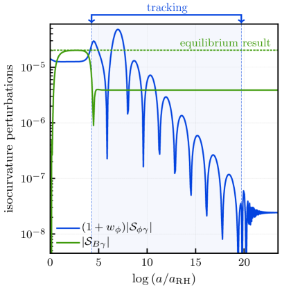
Figure 5: The evolution of both the axionic $\mathcal{S}_{\phi\gamma}$ (blue curve) and baryonic $\mathcal{S}_{B\gamma}$ (green curve) contributions to the isocurvature mode, with a choice of parameters — $m_{\phi}=1~{}\text{eV}$, $mR=10$, $f_{\text{eff}}=10^{13}\,\text{GeV}$, $\theta_{\text{in}}=3/4$, $H_{I}=10^{8}\,\text{GeV}$ — similar to previous figures. The dashed-green curve shows the result in Eq. (92), if spontaneous baryogenesis had occurred at equilibrium, and the shaded-blue area indicates the tracking phase, suppressing as $\mathcal{S}_{\phi\gamma}\propto 1/\sqrt{a}$ over its duration.

III.4.3 Axionic contribution

There are several significant observations to make that are unique to the axionic contribution. To simplify the discussion, we momentarily ignore the baryonic component and define two gauge-invariant entropy perturbations. One is intrinsic Kodama and Sasaki (1984):

$$\Gamma\equiv\frac{\delta P_{\phi}/\rho_{\phi}-c_{\phi}^{2}\delta_{\phi}}{1-c_{\phi}^{2}}\ ,$$ (87)

where $c_{\phi}^{2}\equiv\dot{P}_{\phi}/\dot{\rho}_{\phi}$ is the adiabatic sound speed of the axion fluid. The other is expressed relative to photons:

$$\mathcal{S}_{\phi\gamma}\equiv\frac{\delta_{\phi}}{1+w_{\phi}}-\frac{3}{4}\delta_{\gamma}\ .$$ (88)

The relevant modes for our discussion are outside the Hubble sphere $k\ll aH$ during the early evolution. At these scales, the basis of gauge-invariant perturbations $\{\Phi,\mathcal{R}\}$ and $\{\Gamma,\mathcal{S}_{\phi\gamma}\}$ is convenient, since these two sets decouple. In particular, writing the perturbation equations in this basis and simplifying the system for the tracking regime (i.e., taking $w_{\phi}\rightarrow w=\frac{1}{3}$), we find Bartolo et al. (2004)

$$\frac{1}{2}\frac{d\left[(1+w_{\phi})\mathcal{S}_{\phi\gamma}\right]}{d\log a} =-\Gamma$$

$$2\left[(1+w_{\phi})\mathcal{S}_{\phi\gamma}\right]-\Gamma =\frac{d\Gamma}{d\log a}\ .$$ (89)

The solutions for $\mathcal{S}_{\phi\gamma}$ undergo damped harmonic oscillations every few e-folds, rapidly suppressing the axionic isocurvature amplitude as

$$\mathcal{S}_{\phi\gamma}\propto\frac{1}{\sqrt{a}}\ .$$ (90)

It is instructive to view a numerical solution of the full system of perturbations in this regime, focusing on the tracking period. In Fig. 5 this is shown by the blue curve, where we have highlighted the tracking phase. Indeed, a few e-folds after reheating the axion begins to converge to the tracker solution, and the amplitude of the isocurvature perturbation falls as $1/\sqrt{a}$. The field eventually enters a region of the potential which is approximately harmonic, ending the tracking dynamics and thus concluding the suppression. The isocurvature $\mathcal{S}_{\phi\gamma}$ then undergoes some short-lived transient oscillations before finally settling on its asymptotic late-time value.

III.4.4 Baryonic contribution

The dynamical suppression of $\mathcal{S}_{\phi\gamma}$ is significant, since it could ensure that the baryonic contribution is dominant if tracking lasts for a sufficient number of e-folds. Indeed, this dominance was an assumption we made when deriving the general power spectra in Sec. II.3. The baryonic component is defined in an analogous way:

$$\mathcal{S}_{B\gamma}\equiv\frac{\delta Y_{B}}{Y_{B}}=\delta_{B}-\frac{3}{4}\delta_{\gamma}\ .$$ (91)

An example of numerical solutions for the evolution of $\mathcal{S}_{B\gamma}$ is shown in the solid-green curve of Fig. 5. Apart from some early dynamical behavior as the baryon asymmetry is being established, the $\mathcal{S}_{B\gamma}$ perturbations are essentially fixed after the fast-roll period. However, there are other subtleties that we should outline.

Although the baryon asymmetry is typically produced out-of-equilibrium in this model, a useful benchmark comparison with regard to the perturbation spectrum is the case of in-equilibrium production, which we have shown as a dashed-green line in Fig. 5. We find that the baryonic perturbations for different types of production typically do not differ by more than an order of magnitude throughout most of parameter space. However, there are some particularly important exceptions. To this end, it is instructive to derive an analytical approximation for the equilibrium case in terms of the canonical field $\phi$. Using the proportionality $Y_{B-L}\approx Y_{B-L}^{\text{eq}}\propto\mu_{B-L}T^{2}$ we find the perturbation by evaluating

$$\delta_{B}\approx\frac{\delta\mu_{B-L}}{\mu_{B-L}}=\frac{1}{\mu_{B-L}}\left(\frac{\partial\mu_{B-L}}{\partial\phi}\delta\phi+\frac{\partial\mu_{B-L}}{\partial\dot{\phi}}\delta\dot{\phi}\right)$$ (92)

at the decoupling temperature $T_{\text{D}}$. In previous investigations (e.g., Ref. De Simone and Kobayashi (2016)), a slow-roll approximation is used and neither $\delta\phi$ or $\phi$ are assumed to significantly evolve. Under these conditions, we find an analytical expression:

$$S_{B\gamma}\approx\left.\left\{\frac{2V_{\text{eff}}^{\prime\prime}(\phi)}{V_{\text{eff}}^{\prime}(\phi)}-\frac{V_{\text{eff}}^{\prime}(\phi)}{V_{\text{eff}}(\phi)}\left[\frac{1-\frac{V_{\text{eff}}}{\Lambda^{4}}}{1-\frac{V_{\text{eff}}}{2\Lambda^{4}}}\right]\right\}\right|_{\phi_{\text{in}}}\!\!\frac{H_{I}}{2\pi}\ ,$$ (93)

where the form of the expression is influenced by the chemical potential being a function of both the velocity of the canonical field and the field itself $\mu_{B-L}\propto\dot{\theta}(\phi,\dot{\phi})$. Additionally, note the appearance in Eq. (93) of several critical points for the initial field displacement $\phi_{\text{in}}$: the two terms may have opposite signs, allowing for cancellations and a vanishing $\mathcal{S}_{B\gamma}$, and any inflection points in the canonical potential cause the first term to vanish.

The behavior of the perturbations near these points can dramatically change the isocurvature power spectrum, making the baryonic contribution subdominant. While the perturbations for out-of-equilibrium asymmetry production cannot be found analytically in this way, it is important to investigate how these effects are manifested in that case, which is a question we shall continue to address below.

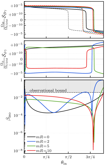
Figure 6: In the top two panels, numerical results for the baryonic and axionic contributions to the isocurvature power $\mathcal{P}_{\mathcal{S}\mathcal{S}}(k_{*})$ are shown, respectively, as a function of the misalignment angle $\theta_{\text{in}}$, with the various curves showing different values of $mR$. The values $f_{\text{eff}}=10^{13}\,\text{GeV}$ and $H_{I}=10^{8}\,\text{GeV}$ were chosen, and $m_{\phi}$ is set to satisfy $\Omega_{\phi}\approx\Omega_{\text{DM}}^{\text{obs}}$. In the top panel, dashed curves show the approximate equilibrium result of Eq. (93). In the bottom panel, the isocurvature fraction $\beta_{\text{iso}}$ is computed for each curve, comprising the total effect.

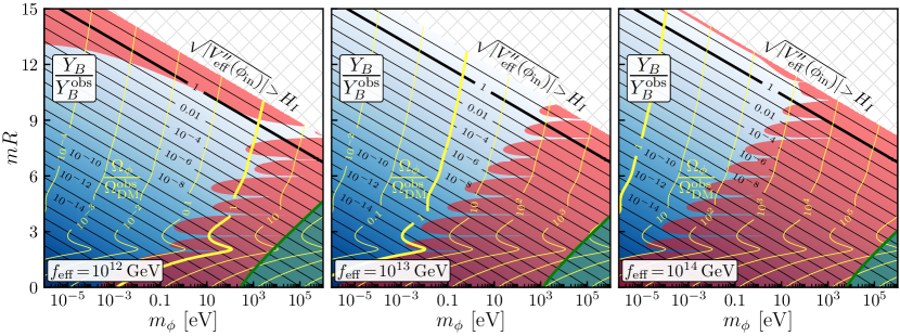
Figure 7: The result from Fig. 4, now including exclusion regions from isocurvature constraints (in red).

III.4.5 Isocurvature bounds

The constraint on isocurvature from the CMB comes in the form of an upper-bound on the uncorrelated “isocurvature fraction,” from Planck collaboration data Akrami et al. (2018):

$$\beta_{\text{iso}}(k_{*})\equiv\frac{\mathcal{P}_{\mathcal{SS}}(k_{*})}{\mathcal{P}_{\mathcal{RR}}(k_{*})+\mathcal{P}_{\mathcal{SS}}(k_{*})}<0.038\ ,$$ (94)

in which $\mathcal{P}_{\mathcal{RR}}(k_{*})\approx 2.10\times 10^{-9}$ is the adiabatic power, $\mathcal{P}_{\mathcal{SS}}(k_{*})$ is the isocurvature power, and each is evaluated at the pivot scale $k_{*}\equiv 0.05~{}\text{Mpc}$. The baryonic and axionic contributions are exactly correlated due to their common source, and appear as a weighted sum

$$\mathcal{P}_{\mathcal{SS}}(k)\equiv\left[\frac{\Omega_{\phi}}{\Omega_{\text{CDM}}}\mathcal{S}_{\phi\gamma}(k)+\frac{\Omega_{B}}{\Omega_{\text{CDM}}}\mathcal{S}_{B\gamma}(k)\right]^{2}\ ,$$ (95)

where $\Omega_{B}\approx 0.0486$ and $\Omega_{\text{CDM}}\approx 0.2589$ are the cosmological abundances for baryons and cold dark matter (CDM), respectively.

Note that the total power spectrum $\mathcal{P}_{\mathcal{S}\mathcal{S}}$ has the possibility for cancellations between axionic and baryonic components. This type of behavior is made more clear in the context of our model by examining the perturbations as a function of the misalignment angle $\theta_{\text{in}}$. In the bottom panel of Fig. 6, we plot the dependence of $\beta_{\text{iso}}(k_{*})$ on $\theta_{\text{in}}$ by numerically solving the perturbation equations. The upper panels show explicitly how the weighted isocurvature sources in Eq. (95) contribute to the bottom panel. The different curves show various choices for $mR$, while $m_{\phi}$ is taken to ensure the axions have the observed DM abundance $\Omega_{\phi}\approx\Omega_{\text{CDM}}$ at $\theta_{\text{in}}=3\pi/4$ (the value used in all previous figures). We have also included the equilibrium result from Eq. (93) with dashed curves in the top panel. Our interest is mostly in the behavior for at least moderate values of $\theta_{\text{in}}$, to ensure the field is misaligned sufficiently from the minimum to enable adequate production of baryon asymmetry.

In the $mR=0$ case of Fig. 6, the axionic isocurvature is monotonic with $\theta_{\text{in}}$ and does not experience any sign changes. However, as $mR$ is increased both isocurvature contributions show vanishing points that generally do not coincide. We also confirm that as $mR$ is increased tracking effects suppress the axionic component, as seen through the overall reduction in the $\mathcal{S}_{\phi\gamma}$ amplitude. The effect is more subtle toward the edge of field space, however, as both contributions are enhanced with $\theta_{\text{in}}$. The accumulation of all the effects is that as we deform the potential, the baryon asymmetry is amplified exponentially as $e^{\pi mR}$, while the isocurvature is increasingly suppressed at moderately large misalignment angles, focused roughly around the $\theta_{\text{in}}\sim 3\pi/4$ region.

While these discussions are instructive in forming a qualitative picture of the perturbations, our interest ultimately is in producing exclusion regions over the plots in Fig. 4. Therefore, we solve the perturbation equations over the full parameter space and mark regions that violate Eq. (94). These are indicated by dark-red in Fig. 7, while all other features and parameter choices are identical to Fig. 4, as discussed previously. We immediately observe that the viable regions in which the baryon abundance $Y_{B}$ (black contours) and axion abundance $\Omega_{\phi}$ (yellow contours) are produced in the observed amounts remain safely outside the exclusion region.

IV Discussion and Conclusions

In this paper, we have investigated the possibility that both the baryon asymmetry of the universe and dark matter may be accounted for by a single axion-like field. In this scenario, the early-universe dynamics of the axion drive a period of spontaneous baryogenesis, during which the observed baryon asymmetry is produced. As the axion field settles to the minimum of its potential, it undergoes coherent oscillations, which behave cosmologically as dark matter at late times. Typically, to generate the observed baryon asymmetry, a relatively “steep” axion potential is required in the region where the axion initially rolls. The corresponding axion mass is large and highly unstable against decays, making it inadequate as a dark matter candidate. However, we have shown that a field-dependent wavefunction renormalization can arise which effectively “deforms” the axion potential, inducing in a mismatch in curvature between different regions. In this way, novel possibilities have emerged, as we can not only generate the observed baryon and dark matter abundance jointly, but the axion dynamics can also exhibit dramatic modifications.

In Sec. II, we have given a general description of the type of wavefunction renormalization necessary to realize such a scenario. Namely, with an enhancement $Z(\theta\lesssim\epsilon)\simeq 1/\epsilon^{2n}$ near the minimum of the axion potential, and $Z(\theta\simeq\theta_{\text{in}})=\mathcal{O}(1)$ near the edges, the necessary deformations in the canonical potential are generated. Specifically, for $\epsilon\ll 1$ this has the effect of flattening the potential near its minimum while leaving its shape toward the edges of field space unaltered. The late-time mass is then suppressed by a factor of $\epsilon^{n}$, while the effective chemical potential which efficiently drives spontaneous baryogenesis is retained. Moreover, the wavefunction enhancement also has the effect of suppressing the axion decay width by a factor of $\epsilon^{2n}$. As we have discussed, the culmination of these features is that the general arrangement in Sec. II can yield the observed baryon asymmetry, while maintaining a sufficiently light and stable axion dark matter candidate. We have investigated the production of baryon asymmetry — both in-equilibrium and out-of-equilibrium — and found that both cases present compelling possibilities.

Meanwhile, to interpolate between the two regions of the wavefunction, we implemented a simple power-law form $Z(\theta)\simeq 1/\theta^{2n}$. As a result, we have shown that the axion exhibits a “tracking” behavior as it transits through this region. The field follows an attractor-like trajectory in which its late-time evolution is made increasingly insensitive to initial conditions. This phenomenon implies not only an axion relic abundance which is insensitive to the initial misalignment angle, but also a suppression of its isocurvature perturbations. We also have described how the axion equation-of-state parameter during this period converges to a non-trivial value $w_{\phi}\rightarrow(1+w-n)/n$, which reflects the shape of the potential through its dependence on the parameter $n$.

In Sec. III, we have supplied a “proof of concept” by constructing an explicit model using the five-dimensional continuum-clockwork axion, which serves as a realization of the more general scenario described in Sec. II. In particular, by integrating out the heavy KK modes and examining the theory for the lightest four-dimensional axion, we have shown that such a model furnishes a wavefunction renormalization $Z(\theta)$ with similar properties to the $n=1$ case of Sec. II. The small parameter $\epsilon$ that determines the deformation of the axion potential is mapped onto a factor $e^{\pi mR}$ in the clockwork theory, such that the scale of bulk and boundary masses $m$ and the size of the extra dimension $R$ together set the strength of the deformation. We have shown (see, for example, Fig. 3) that spontaneous baryogenesis in this model is typically accomplished via out-of-equilibrium production, in contrast to many of the conventional spontaneous baryogenesis models in the literature. Moreover, we have also recovered the anticipated tracking dynamics in this model, as the clockwork parameters exceed $mR\gtrsim\mathcal{O}(\text{few})$. We have determined regions of phenomenological viability by producing a set of numerical simulations over the parameter space. Namely, in Fig. 4 we have shown the produced baryon asymmetry and axion relic abundance over a range of parameters and found several viable regions.

We have also, at the close of Sec. III, given a more thorough treatment of the large-scale isocurvature perturbations produced in this model, which include both axionic and baryonic components. The evolution of these components in the early universe is made non-trivial by the deformations to the potential. As anticipated in Sec. II, the axionic component is suppressed by tracking dynamics, and we have determined that in most regions the baryonic isocurvature component is dominant. Furthermore, we have demonstrated an interesting dependence of the perturbations on the initial misalignment angle $\theta_{\text{in}}$. There are certain critical points for $\theta_{\text{in}}$ where sign-changes can occur in the amplitude of either of the perturbation components, which can result in a suppression in that region. These points generally shift throughout the model parameter space. The culmination of these effects is a non-trivial bound imposed by the CMB isocurvature constraints. Although these bounds can be quite severe, we have found that the viable regions for the CCW model all remain below the isocurvature constraints (see Fig. 7).

To conclude, we have shown in this paper that an axion with a field-dependent wavefunction renormalization, which is enhanced near the minimum of the axion potential, can generate both the observed baryon asymmetry and dark matter relic abundance. Using the continuum-clockwork axion, we have constructed an explicit model realization of this idea. Our results also suggest directions for further research, including approaches with multiple scalar fields, where non-trivial dynamics can arise that significantly alters the effective chemical potential, e.g., effects from temperature-dependent masses Dienes et al. (2016, 2017). Moreover, the CCW axion model constitutes only a single realization of the more general idea in this paper. A natural extension is to explore other models which yield similar non-canonical kinetic terms, but an altogether different set of phenomenological possibilities.

Appendix A Tracking Dynamics

In this appendix, we provide a short review on cosmological tracking solutions and their general classification in terms of the scalar field potential. Throughout much of this review we closely follow the methodology and results of Ref. Steinhardt et al. (1999). We first give the necessary background for Sec. II and the formalism used to deduce the class of potentials and regions in field space which exhibit tracking solutions [see Eq. (15)]. Then, we tailor our analysis specifically to the continuum-clockwork axion example of Sec III, showing that tracking solutions are a generic property of these potentials which drive the axion equation of state to that of the background $w_{\phi}\rightarrow w$.

A.1 Classification of Tracking Potentials

A tracking field, by definition, is a field that converges to a given evolution in phase space, even under a variation in initial conditions. Typically, such attractor-like solutions are also associated with convergence of the equation-of-state parameter $w_{\phi}$ to some fixed value, but this ultimately depends on the background cosmology.

Let us consider a canonically normalized scalar field $\phi$ with potential $V(\phi)$ that evolves in an FRW spacetime:

$$\ddot{\phi}+3H\dot{\phi}+V^{\prime}(\phi)=0\ .$$ (96)

A useful parameter to define is the ratio of kinetic energy to potential energy of the scalar field:

$$x\equiv\frac{\frac{1}{2}\dot{\phi}^{2}}{V(\phi)}=\frac{1+w_{\phi}}{1-w_{\phi}}\ .$$ (97)

After some rearrangement, Eq. (96) can be recast as

$$\frac{1}{6}\frac{d\log x}{d\log a}=M_{P}\sqrt{\frac{\Omega_{\phi}}{3(1+w_{\phi})}}\left|\frac{V^{\prime}(\phi)}{V(\phi)}\right|-1\ .$$ (98)

A tracking solution with a convergent equation of state requires that $x$ is approximately constant, such that the last term is small. The expression

$$\left|\frac{V^{\prime}(\phi)}{V(\phi)}\right|\approx\frac{1}{M_{P}}\sqrt{\frac{3(1+w_{\phi})}{\Omega_{\phi}}}\approx\frac{H}{\big{|}\dot{\phi}\big{|}}$$ (99)

then dictates the tracking trajectory, where in the last approximation we implicitly assumed $1+w_{\phi}=\mathcal{O}(1)$.

Naturally, for the tracking condition in Eq. (99) to remain satisfied as the system evolves, both sides of the relation must change in the same way. Therefore, differentiating the equation of motion with respect to $\phi$, and demanding still that $x$ varies negligibly with time, we arrive at the relation

$$\Gamma\equiv\frac{V^{\prime\prime}(\phi)V(\phi)}{\left[V^{\prime}(\phi)\right]^{2}}\approx 1+\frac{w-w_{\phi}}{2(1+w_{\phi})}\ .$$ (100)

The necessary (but not sufficient) condition is that a region of the potential may yield tracking solutions if the dimensionless quantity $\Gamma$ does not vary appreciably over that field range. It acts as a determinant for classifying the features of different tracking regions and it does this only through properties of the potential, without reference to any dynamical information. In particular, the equation-of-state parameter to which the tracker converges is found by rearranging the above expression:

$$w_{\phi}\approx\frac{w-2(\Gamma-1)}{1+2(\Gamma-1)}\ ,$$ (101)

which is determines the evolution of $\Omega_{\phi}$ during tracking.

The condition in Eq. (100) is not always sufficient because it does not guarantee that the tracking solutions are stable under small perturbations to the equation of state. An analysis shows that

$$\Gamma>1-\frac{1-w}{6+2w}\geq\frac{1}{2}$$ (102)

is required for stable tracking solutions. Moreover, within the above range there are two distinctive behaviors. In the case that $\Gamma>1$, the equation of state for the scalar field is less kinetic than the background $w_{\phi}<w$, so the abundance $\Omega_{\phi}$ grows during tracking. On the other hand, in the $\Gamma<1$ case we find $w_{\phi}>w$ instead, and the abundance falls during that epoch. The “borderline” scenario of $\Gamma=1$ is also an interesting critical case for which $w_{\phi}$ is driven to match the background, and $\Omega_{\phi}$ does not evolve at all. This borderline case is found with potentials that have an exponential region. Incidentally, this is approximately the scenario we find in the continuum-clockwork axion example of Sec. III, for which we now briefly specialize our discussion.

A.2 Tracking with Continuum-Clockwork Axion

Let us now examine the continuum-clockwork example of Sec. III and use the analysis above the identify any tracking regions for that potential. It is perhaps instructive to first consider $mR=0$, i.e., the standard sinusoidal axion potential $V_{\text{eff}}(\phi)=\Lambda^{4}[1-\cos(\phi/f)]$. Using the definition in Eq. (100) we find that

$$\Gamma=1-\frac{1}{1+\cos\left(\frac{\phi}{f}\right)}\ .$$ (103)

Regardless of how slowly this function varies throughout field space, it is bounded from above by $\Gamma\leq\frac{1}{2}$ and thus never can admit stable tracking solutions.

On the other hand, allowing for $mR>0$ sufficiently large such that $e^{-2\pi mR}\ll 1$, we can approximate

$$\Gamma\approx 1-\frac{1}{2}\text{sech}^{2}\!\!\left(\frac{\phi}{2f}\right)<1\ .$$ (104)

Although $\Gamma$ is always less than unity, for field values larger than $\phi/f\gtrsim 3$ we can achieve $\Gamma>\frac{9}{10}$ and thus find stable tracking solutions. This is easy to accomplish for $\phi\sim f_{\text{eff}}$ if $mR$ is moderately large. Additionally, we must check that $\Gamma$ is slowly varying over a Hubble time:

$$\left|\frac{1}{\Gamma}\frac{d\Gamma}{dN_{e}}\right|\approx\left|\text{sech}\!\left(\frac{\phi}{f}\right)\right|\tanh^{2}\!\!\left(\frac{\phi}{2f}\right)\ll 1\ ,$$ (105)

where $N_{e}$ is the number of efolds and we used Eq. (99). In the field range where Eq. (104) is viable, the above condition is easily satisfied as well, and we can therefore always identify a tracking region of the CCW axion potential for $e^{-2\pi mR}\ll 1$.

Indeed, the above analysis confirms the findings of our numerical simulations in Sec. III, including the fact that the axion equation of state always appears radiation-like during the tracking period. Using Eq. (101), we find

$$w_{\phi}\approx w+\left(1+w\right)\text{csch}^{2}\!\left(\frac{\phi}{2f}\right)\ ,$$ (106)

which in the proper field range matches the background $w_{\phi}\approx w$ to an excellent approximation.

Appendix B Boltzmann Equations for $B-L$ at High Temperature

In this appendix, we derive the effective chemical potential $\mu_{B-L}$ used in Eq. (35), taking into account the details of sphaleron transitions in the Boltzmann evolution. To begin, let us consider a species $X$ which is in kinetic equilibrium at temperature $T$. Assuming some chemical potential $\mu_{X}$, the asymmetry in number density between particles and antiparticles is described by either Fermi-Dirac $(+)$ or Bose-Einstein $(-)$ statistics as

$$n_{X}=g_{X}\int\frac{d^{3}\vec{p}}{(2\pi)^{3}} \left[\frac{1}{\exp\left[\left(E_{X}-\mu_{X}\right)/T\right]\pm 1}\right.$$

$$\hskip 5.69054pt-\left.\frac{1}{\exp\left[\left(E_{X}+\mu_{X}\right)/T\right]\pm 1}\right]\ ,$$ (107)

where $g_{X}$ is the number of degrees of freedom for the species and $E_{X}=\sqrt{p^{2}+m_{X}^{2}}$ is the energy. At high temperature $T\gg(\mu_{X},m_{X}\!)$, this is well-approximated by

$$n_{X}\approx\left\{\begin{array}[]{ll}g_{X}\mu_{X}T^{2}/6&\ \ \text{for fermions}\\ g_{X}\mu_{X}T^{2}/3&\ \ \text{for bosons}\end{array}\right.\ ,$$ (108)

such that a proportionality exists between the chemical potential and the number density for the species.

Let us now consider that this species is involved in some chemical process $A$, according to

$$A:\ \ X+i+\cdots\ \longleftrightarrow\ j+\cdots\ .$$ (109)

Naturally, if the reaction is sufficiently rapid and it reaches chemical equilibrium, then the associated chemical potentials satisfy algebraic relations

$$d_{A,X}\,\mu_{X}+d_{A,i}\,\mu_{i}+d_{A,j}\,\mu_{j}+\cdots=0\ ,$$ (110)

where $d_{A,X}$ ($d_{A,i}$) denotes the multiplicity of $X$ ​($i$) and the signs determine the direction of the reaction. In the case of a spatially homogeneous and spontaneous violation of $CPT$ symmetry, as studied in this paper, these relations are sourced by an effective chemical potential $\mu_{A}$. That is, we instead have the relations

$$d_{A,X}\mu_{X}+d_{A,i}\mu_{i}+d_{A,j}\mu_{j}+\cdots+\mu_{A}=0\ .$$ (111)

The corresponding out-of-equilibrium evolution for the number density $n_{X}$ is given by the Boltzmann equation

$$\dot{n}_{X} +3Hn_{X}$$ (112)

$$=-\sum_{A}d_{A,X}\gamma_{A}\left(d_{A,X}\,\frac{\mu_{X}}{T}+d_{A,i}\,\frac{\mu_{i}}{T}+\cdots+\frac{\mu_{A}}{T}\right)\ .$$

where $\gamma_{A}$ is the thermally averaged interaction rate density for the process $A$ normalized by $T^{3}$, and the sum is over all the chemical processes involving $X$. We can solve the coupled Boltzmann equations with some set of sources $\{\mu_{A}\}$ and obtain any of the number densities or chemical potentials in the process, e.g., the lepton- and baryon-number density $n_{L}$ and $n_{B}$.

Considering that all processes preserve the gauge symmetry $\text{SU}(3)_{c}\times\text{SU}(2)_{W}\times\text{U}(1)_{Y}$ during baryogenesis, the chemical potentials for the gauge bosons all vanish, and we can impose other additional constraints. In particular, the expectation value for the hypercharge $\langle Y\rangle$ over the chemical potentials should vanish:

$$\sum_{i}(\mu_{q_{i}}+2\mu_{u_{i}}-\mu_{d_{i}}-\mu_{\ell_{i}}-\mu_{e_{i}})+2\mu_{\mathcal{H}}=0\ ,$$ (113)

where, respectively, $i$ is a flavor index, $q$ and $\ell$ are left-handed quark and lepton doublets, $u$ and $d$ are right-handed up and down quarks, $e$ is a right-handed electron, and $\mathcal{H}$ is the Higgs boson.

Under the above constraint, we can show that the quark number densities evolve according to

$$\dot{n}_{q_{i}}+3Hn_{q_{i}}= -\frac{\gamma_{\lambda_{u_{i}}}}{T}\left(\mu_{q_{i}}-\mu_{u_{i}}+\mu_{\mathcal{H}}\right)$$

$$-\frac{\gamma_{\lambda_{d_{i}}}}{T}\left(\mu_{q_{i}}-\mu_{d_{i}}-\mu_{\mathcal{H}}\right)$$

$$-2\frac{\gamma_{\text{ss}}}{T}\sum_{j}\left(2\mu_{q_{j}}-\mu_{u_{j}}-\mu_{d_{j}}\right)$$

$$-3\frac{\gamma_{\text{ws}}}{T}\Big{[}\sum_{j}\left(3\mu_{q_{j}}+\mu_{\ell_{j}}\right)+\mu_{\text{ws}}\Big{]}$$ (114)

and

$$\dot{n}_{u_{i}}+3Hn_{u_{i}}= \phantom{+}\frac{\gamma_{\lambda_{u_{i}}}}{T}\left(\mu_{q_{i}}-\mu_{u_{i}}+\mu_{\mathcal{H}}\right)$$

$$+\frac{\gamma_{\text{ss}}}{T}\sum_{j}\left(2\mu_{q_{j}}-\mu_{u_{j}}-\mu_{d_{j}}\right)$$

$$\dot{n}_{d_{i}}+3Hn_{d_{i}}= \phantom{+}\frac{\gamma_{\lambda_{d_{i}}}}{T}\left(\mu_{q_{i}}-\mu_{d_{i}}-\mu_{\mathcal{H}}\right)$$

$$+\frac{\gamma_{\text{ss}}}{T}\sum_{j}\left(2\mu_{q_{j}}-\mu_{u_{j}}-\mu_{d_{j}}\right)\ ,$$ (115)

while the lepton number densities evolve as

$$\dot{n}_{\ell_{i}}+3Hn_{\ell_{i}}= -\frac{\gamma_{\lambda_{e_{i}}}}{T}\left(\mu_{\ell_{i}}-\mu_{e_{i}}-\mu_{\mathcal{H}}\right)$$

$$-\frac{\gamma_{\text{ws}}}{T}\Big{[}\sum_{j}\left(3\mu_{q_{j}}+\mu_{\ell_{j}}\right)+\mu_{\text{ws}}\Big{]}$$

$$-\sum_{j}\frac{{\gamma_{L\hskip-4.26773pt/}}_{ij}}{T}\left(\mu_{\ell_{i}}+\mu_{\ell_{j}}+2\mu_{\mathcal{H}}\right)$$

$$\dot{n}_{e_{i}}+3Hn_{e_{i}}= \phantom{+}\frac{\gamma_{\lambda_{e_{i}}}}{T}\left(\mu_{\ell_{i}}-\mu_{e_{i}}-\mu_{\mathcal{H}}\right)\ .$$ (116)

In the above, the rate densities $\gamma_{\lambda_{u_{i}}}$, $\gamma_{\lambda_{d_{i}}}$, and $\gamma_{\lambda_{e_{i}}}$ correspond to Yukawa interactions in the SM, while the other rate densities $\gamma_{\text{ss}}$ and $\gamma_{\text{ws}}$ correspond to strong and weak sphalerons. The source of $(B-L)$ violation in this paper is the Weinberg operator in Eq. (30), for which we denote the rate density as ${\gamma_{L\hskip-4.26773pt/}}_{ij}$. The one remaining unspecified quantity $\mu_{\text{ws}}$ is related to the spontaneous breaking of the $CPT$ symmetry through Eq. (28). As the axion field rolls down its potential, it induces this effective chemical potential for the weak sphalerons:

$$\mu_{\text{ws}}=\partial_{0}\theta\ .$$ (117)

Adding the various contributions from the Boltzmann equations above, we can determine the number-density evolution for baryons $n_{B}$ and leptons $n_{L}$ as

$$\dot{n}_{B}+3Hn_{B}= -3\frac{\gamma_{\text{ws}}}{T}\Big{[}\sum_{i}(3\mu_{q_{i}}+\mu_{\ell_{i}})+\mu_{\text{ws}}\Big{]}$$

$$\dot{n}_{L}+3Hn_{L}= -3\frac{\gamma_{\text{ws}}}{T}\Big{[}\sum_{i}(3\mu_{q_{i}}+\mu_{\ell_{i}})+\mu_{\text{ws}}\Big{]}$$

$$-\sum_{ij}\frac{{\gamma_{L\hskip-4.26773pt/}}_{ij}}{T}(\mu_{\ell_{i}}+\mu_{\ell_{j}}+2\mu_{\mathcal{H}})\ .$$ (118)

It is instructive to comment on the limit where the weak sphaleron rate is negligibly small. Taking $\gamma_{\text{ws}}\rightarrow 0$ in these equations, we find that the evolution of $n_{B}$ becomes trivial and that $n_{B}=0$ if the initial baryon number is zero. In this limit, the equation for lepton number also loses source terms, implying $n_{L}$ is also vanishing Shi and Raby (2015).

With the hypercharge constraint from Eq. (113), and vanishing initial conditions $\{\mu_{i}=0\}$, we can in principle solve the coupled Boltzmann equations numerically. However, we can also simplify them through some physical considerations. Let us assume that the Yukawa interactions for $N_{f}$ generations of fermions are in equilibrium, in addition to all gauge interactions and the strong and weak sphalerons. However, we shall ignore the Yukawa interactions of the remaining $3-N_{f}$ generations during baryogenesis. In such a case, baryon and lepton number are mostly generated by sphaleron processes in conjunction with axion dynamics, which leads approximately to the flavor-universal contributions

$$n_{B_{i}}\simeq\frac{1}{3}n_{B}\qquad n_{L_{i}}\simeq\frac{1}{3}n_{L}\ .$$ (119)

Furthermore, the interactions that violate $(B-L)$ are not flavor-diagonal. Instead, they are flavor-democratic, such that the off-diagonal components are determined by the PMNS neutrino mixing matrix. We can therefore simplify the $(B-L)$ rate density to

$${\gamma_{L\hskip-4.26773pt/}}_{ij}\simeq\gamma_{L\hskip-4.26773pt/}\ ,$$ (120)

for all lepton flavors, where we defined $\gamma_{L\hskip-4.26773pt/}$ in Eq. (34).

Taking these simplifications into account, we can compute the necessary chemical potentials. In particular, for the Higgs we find

$$\mu_{\mathcal{H}}=\frac{(9+N_{f})n_{L}-9n_{B}}{2(3+5N_{f})T^{2}}\ ,$$ (121)

while for the $N_{f}$ generations of quarks and leptons with Yukawa interactions in equilibrium we have

$$\mu_{u_{i}} =\frac{(9+N_{f})n_{L}-(6-5N_{f})n_{B}}{2(3+5N_{f})T^{2}}$$

$$\mu_{d_{i}} =\frac{(12+5N_{f})n_{B}-(9+N_{f})n_{L}}{2(3+5N_{f})T^{2}}$$

$$\mu_{\ell_{i}} =\frac{7(1+N_{f})n_{L}-3n_{B}}{2(3+5N_{f})T^{2}}$$

$$\mu_{e_{i}} =\frac{3n_{B}-(1-3N_{f})n_{L}}{(3+5N_{f})T^{2}}\ .$$ (122)

and for the remaining $3-N_{f}$ generations:

$$\mu_{u_{i}}=\mu_{d_{i}} =\frac{n_{B}}{2T^{2}}$$

$$\mu_{\ell_{i}} =\frac{n_{L}}{T^{2}}$$

$$\mu_{e_{i}} =0\ .$$ (123)

Meanwhile, the chemical potential for the left-handed quark doublets is independent of $N_{f}$:

$$\mu_{q_{i}}=\frac{n_{B}}{2T^{2}}\ .$$ (124)

The $n_{B}$ and $n_{L}$ number densities are related to each other by weak sphaleron processes:

$$n_{B} =\frac{(18+31N_{f}-3N_{f}^{2})n_{B-L}-2(3+5N_{f})\mu_{\text{ws}}T^{2}}{45+73N_{f}-3N_{f}^{2}}$$

$$n_{L} =\frac{-3(9+14N_{f})n_{B-L}-2(3+5N_{f})\mu_{\text{ws}}T^{2}}{45+73N_{f}-3N_{f}^{2}}\ .$$ (125)

The evolution of $n_{B-L}$ is determined by the difference between the equations in Eq. (B) and the chemical potentials above:

$$\dot{n}_{B-L}+3Hn_{B-L}=-\Gamma_{L\hskip-4.26773pt/}\left(n_{B-L}-n_{B-L}^{\text{eq}}\right)\ ,$$ (126)

where the rate is given by

$$\Gamma_{L\hskip-4.26773pt/}=\frac{9(171+65N_{f}-6N_{f}^{2})}{45+73N_{f}-3N_{f}^{2}}\frac{\gamma_{L\hskip-4.26773pt/}}{T^{3}}$$ (127)

and the equilibrium number density is given by

$$n_{B-L}^{\text{eq}}=-\frac{2(36+65N_{f}-6N_{f}^{2})}{9(171+65N_{f}-6N_{f}^{2})}\mu_{\text{ws}}T^{2}\ .$$ (128)

The above expression provides us with the coefficient that appears in Eq. (35). We are now equipped to compute the final number density $n_{B-L}$ and therefore the final baryon asymmetry. In particular, after the weak sphalerons decouple at $T\lesssim 100\,\text{GeV}$:

$$n_{B}=\frac{28}{79}n_{B-L}\ .$$ (129)

References

- Iocco et al. (2009) F. Iocco, G. Mangano, G. Miele, O. Pisanti, and P. D. Serpico, Phys. Rept. 472, 1 (2009), arXiv:0809.0631 [astro-ph] .
- Ade et al. (2016) P. A. R. Ade et al. (Planck), Astron. Astrophys. 594, A13 (2016), arXiv:1502.01589 [astro-ph.CO] .
- Sakharov (1967) A. D. Sakharov, Pisma Zh. Eksp. Teor. Fiz. 5, 32 (1967), [Usp. Fiz. Nauk161,61(1991)].
- Cohen and Kaplan (1987) A. G. Cohen and D. B. Kaplan, Phys. Lett. B199, 251 (1987).
- Cohen and Kaplan (1988) A. G. Cohen and D. B. Kaplan, Nucl. Phys. B308, 913 (1988).
- Brandenberger and Yamaguchi (2003) R. H. Brandenberger and M. Yamaguchi, Phys. Rev. D68, 023505 (2003), arXiv:hep-ph/0301270 [hep-ph] .
- Takahashi and Yamada (2016) F. Takahashi and M. Yamada, Phys. Lett. B756, 216 (2016), arXiv:1510.07822 [hep-ph] .
- Chiba et al. (2004) T. Chiba, F. Takahashi, and M. Yamaguchi, Phys. Rev. Lett. 92, 011301 (2004), [Erratum: Phys. Rev. Lett.114,no.20,209901(2015)], arXiv:hep-ph/0304102 [hep-ph] .
- Takahashi and Yamaguchi (2004) F. Takahashi and M. Yamaguchi, Phys. Rev. D69, 083506 (2004), arXiv:hep-ph/0308173 [hep-ph] .
- Alberghi et al. (2007) G. L. Alberghi, R. Casadio, and A. Tronconi, Mod. Phys. Lett. A22, 339 (2007), arXiv:hep-ph/0310052 [hep-ph] .
- Li et al. (2002) M.-z. Li, X.-l. Wang, B. Feng, and X.-m. Zhang, Phys. Rev. D65, 103511 (2002), arXiv:hep-ph/0112069 [hep-ph] .
- De Felice et al. (2003) A. De Felice, S. Nasri, and M. Trodden, Phys. Rev. D67, 043509 (2003), arXiv:hep-ph/0207211 [hep-ph] .
- Li and Zhang (2003) M. Li and X. Zhang, Phys. Lett. B573, 20 (2003), arXiv:hep-ph/0209093 [hep-ph] .
- Davoudiasl et al. (2004) H. Davoudiasl, R. Kitano, G. D. Kribs, H. Murayama, and P. J. Steinhardt, Phys. Rev. Lett. 93, 201301 (2004), arXiv:hep-ph/0403019 [hep-ph] .
- Cohen et al. (1991) A. G. Cohen, D. B. Kaplan, and A. E. Nelson, Phys. Lett. B263, 86 (1991).
- Kusenko et al. (2015a) A. Kusenko, L. Pearce, and L. Yang, Phys. Rev. Lett. 114, 061302 (2015a), arXiv:1410.0722 [hep-ph] .
- Carroll and Shu (2006) S. M. Carroll and J. Shu, Phys. Rev. D73, 103515 (2006), arXiv:hep-ph/0510081 [hep-ph] .
- Kusenko et al. (2015b) A. Kusenko, K. Schmitz, and T. T. Yanagida, Phys. Rev. Lett. 115, 011302 (2015b), arXiv:1412.2043 [hep-ph] .
- De Simone and Kobayashi (2016) A. De Simone and T. Kobayashi, JCAP 1608, 052 (2016), arXiv:1605.00670 [hep-ph] .
- De Simone et al. (2017) A. De Simone, T. Kobayashi, and S. Liberati, Phys. Rev. Lett. 118, 131101 (2017), arXiv:1612.04824 [hep-ph] .
- Peccei and Quinn (1977a) R. D. Peccei and H. R. Quinn, Phys. Rev. Lett. 38, 1440 (1977a).
- Peccei and Quinn (1977b) R. D. Peccei and H. R. Quinn, Phys. Rev. D16, 1791 (1977b).
- Weinberg (1978) S. Weinberg, Phys. Rev. Lett. 40, 223 (1978).
- Wilczek (1978) F. Wilczek, Phys. Rev. Lett. 40, 279 (1978).
- Svrcek and Witten (2006) P. Svrcek and E. Witten, JHEP 06, 051 (2006), arXiv:hep-th/0605206 [hep-th] .
- Jaeckel and Ringwald (2010) J. Jaeckel and A. Ringwald, Ann. Rev. Nucl. Part. Sci. 60, 405 (2010), arXiv:1002.0329 [hep-ph] .
- Rubin (2001) S. G. Rubin, JETP Lett. 74, 247 (2001), [Pisma Zh. Eksp. Teor. Fiz.74,275(2001)], arXiv:hep-ph/0110132 [hep-ph] .
- Tolley and Wyman (2010) A. J. Tolley and M. Wyman, Phys. Rev. D81, 043502 (2010), arXiv:0910.1853 [hep-th] .
- Dong et al. (2011) X. Dong, B. Horn, E. Silverstein, and A. Westphal, Phys. Rev. D84, 026011 (2011), arXiv:1011.4521 [hep-th] .
- Bezrukov and Shaposhnikov (2008) F. L. Bezrukov and M. Shaposhnikov, Phys. Lett. B659, 703 (2008), arXiv:0710.3755 [hep-th] .
- Kallosh et al. (2014) R. Kallosh, A. Linde, and D. Roest, Phys. Rev. Lett. 112, 011303 (2014), arXiv:1310.3950 [hep-th] .
- Armendariz-Picon et al. (1999) C. Armendariz-Picon, T. Damour, and V. F. Mukhanov, Phys. Lett. B458, 209 (1999), arXiv:hep-th/9904075 [hep-th] .
- Alishahiha et al. (2004) M. Alishahiha, E. Silverstein, and D. Tong, Phys. Rev. D70, 123505 (2004), arXiv:hep-th/0404084 [hep-th] .
- Domcke et al. (2017) V. Domcke, F. Muia, M. Pieroni, and L. T. Witkowski, JCAP 1707, 048 (2017), arXiv:1704.03464 [astro-ph.CO] .
- Chiba et al. (2000) T. Chiba, T. Okabe, and M. Yamaguchi, Phys. Rev. D62, 023511 (2000), arXiv:astro-ph/9912463 [astro-ph] .
- Armendariz-Picon et al. (2000) C. Armendariz-Picon, V. F. Mukhanov, and P. J. Steinhardt, Phys. Rev. Lett. 85, 4438 (2000), arXiv:astro-ph/0004134 [astro-ph] .
- Armendariz-Picon et al. (2001) C. Armendariz-Picon, V. F. Mukhanov, and P. J. Steinhardt, Phys. Rev. D63, 103510 (2001), arXiv:astro-ph/0006373 [astro-ph] .
- Alonso-Álvarez and Jaeckel (2018) G. Alonso-Álvarez and J. Jaeckel, Phys. Rev. D98, 023539 (2018), arXiv:1712.07500 [hep-ph] .
- Kawasaki et al. (2011) M. Kawasaki, T. Kobayashi, and F. Takahashi, Phys. Rev. D84, 123506 (2011), arXiv:1107.6011 [astro-ph.CO] .
- Wetterich (1988) C. Wetterich, Nucl. Phys. B302, 668 (1988), arXiv:1711.03844 [hep-th] .
- Ratra and Peebles (1988) B. Ratra and P. J. E. Peebles, Phys. Rev. D37, 3406 (1988).
- Zlatev et al. (1999) I. Zlatev, L.-M. Wang, and P. J. Steinhardt, Phys. Rev. Lett. 82, 896 (1999), arXiv:astro-ph/9807002 [astro-ph] .
- Steinhardt et al. (1999) P. J. Steinhardt, L.-M. Wang, and I. Zlatev, Phys. Rev. D59, 123504 (1999), arXiv:astro-ph/9812313 [astro-ph] .
- Witten (1984) E. Witten, Phys. Lett. 149B, 351 (1984).
- Green and Schwarz (1984) M. B. Green and J. H. Schwarz, Phys. Lett. 149B, 117 (1984).
- Choi and Kim (1985a) K. Choi and J. E. Kim, Phys. Lett. 154B, 393 (1985a), [Erratum: Phys. Lett.156B,452(1985)].
- Witten (1985) E. Witten, Phys. Lett. 153B, 243 (1985).
- Choi and Kim (1985b) K. Choi and J. E. Kim, Phys. Lett. 165B, 71 (1985b).
- Fukugita and Yanagida (1986) M. Fukugita and T. Yanagida, Phys. Lett. B174, 45 (1986).
- Hall et al. (2010) L. J. Hall, K. Jedamzik, J. March-Russell, and S. M. West, JHEP 03, 080 (2010), arXiv:0911.1120 [hep-ph] .
- Akrami et al. (2018) Y. Akrami et al. (Planck), (2018), arXiv:1807.06211 [astro-ph.CO] .
- Giudice and McCullough (2017a) G. F. Giudice and M. McCullough, JHEP 02, 036 (2017a), arXiv:1610.07962 [hep-ph] .
- Craig et al. (2017) N. Craig, I. Garcia Garcia, and D. Sutherland, JHEP 10, 018 (2017), arXiv:1704.07831 [hep-ph] .
- Giudice and McCullough (2017b) G. F. Giudice and M. McCullough, (2017b), arXiv:1705.10162 [hep-ph] .
- Choi et al. (2017) K. Choi, S. H. Im, and C. S. Shin, (2017), arXiv:1711.06228 [hep-ph] .
- Kim et al. (2005) J. E. Kim, H. P. Nilles, and M. Peloso, JCAP 0501, 005 (2005), arXiv:hep-ph/0409138 [hep-ph] .
- Choi et al. (2014) K. Choi, H. Kim, and S. Yun, Phys. Rev. D90, 023545 (2014), arXiv:1404.6209 [hep-th] .
- Choi and Im (2016) K. Choi and S. H. Im, JHEP 01, 149 (2016), arXiv:1511.00132 [hep-ph] .
- Kaplan and Rattazzi (2016) D. E. Kaplan and R. Rattazzi, Phys. Rev. D93, 085007 (2016), arXiv:1511.01827 [hep-ph] .
- Higaki et al. (2016a) T. Higaki, K. S. Jeong, N. Kitajima, and F. Takahashi, Phys. Lett. B755, 13 (2016a), arXiv:1512.05295 [hep-ph] .
- Higaki et al. (2016b) T. Higaki, K. S. Jeong, N. Kitajima, and F. Takahashi, JHEP 06, 150 (2016b), arXiv:1603.02090 [hep-ph] .
- Higaki et al. (2016c) T. Higaki, K. S. Jeong, N. Kitajima, T. Sekiguchi, and F. Takahashi, JHEP 08, 044 (2016c), arXiv:1606.05552 [hep-ph] .
- Farina et al. (2017) M. Farina, D. Pappadopulo, F. Rompineve, and A. Tesi, JHEP 01, 095 (2017), arXiv:1611.09855 [hep-ph] .
- Coy et al. (2017) R. Coy, M. Frigerio, and M. Ibe, JHEP 10, 002 (2017), arXiv:1706.04529 [hep-ph] .
- Long (2018) A. J. Long, JHEP 07, 066 (2018), arXiv:1803.07086 [hep-ph] .
- Hambye et al. (2017) T. Hambye, D. Teresi, and M. H. G. Tytgat, JHEP 07, 047 (2017), arXiv:1612.06411 [hep-ph] .
- Kim and McDonald (2018) J. Kim and J. McDonald, Phys. Rev. D98, 023533 (2018), arXiv:1709.04105 [hep-ph] .
- Kim and Mcdonald (2018) J. Kim and J. Mcdonald, (2018), arXiv:1804.02661 [hep-ph] .
- Goudelis et al. (2018) A. Goudelis, K. A. Mohan, and D. Sengupta, (2018), arXiv:1807.06642 [hep-ph] .
- Fonseca et al. (2016) N. Fonseca, L. de Lima, C. S. Machado, and R. D. Matheus, Phys. Rev. D94, 015010 (2016), arXiv:1601.07183 [hep-ph] .
- Saraswat (2017) P. Saraswat, Phys. Rev. D95, 025013 (2017), arXiv:1608.06951 [hep-th] .
- Kehagias and Riotto (2017) A. Kehagias and A. Riotto, Phys. Lett. B767, 73 (2017), arXiv:1611.03316 [hep-ph] .
- Park and Shin (2018a) S. C. Park and C. S. Shin, (2018a), arXiv:1807.09952 [hep-ph] .
- Agrawal et al. (2018) P. Agrawal, J. Fan, and M. Reece, (2018), arXiv:1806.09621 [hep-th] .
- Hong et al. (2018) D. K. Hong, D. H. Kim, and C. S. Shin, Phys. Rev. D97, 035014 (2018), arXiv:1706.09376 [hep-ph] .
- Park and Shin (2018b) S. C. Park and C. S. Shin, Phys. Lett. B776, 222 (2018b), arXiv:1707.07364 [hep-ph] .
- Ibarra et al. (2018) A. Ibarra, A. Kushwaha, and S. K. Vempati, Phys. Lett. B780, 86 (2018), arXiv:1711.02070 [hep-ph] .
- Alonso et al. (2018) R. Alonso, A. Carmona, B. M. Dillon, J. F. Kamenik, J. Martin Camalich, and J. Zupan, (2018), arXiv:1807.09792 [hep-ph] .
- Ahmed and Dillon (2017) A. Ahmed and B. M. Dillon, Phys. Rev. D96, 115031 (2017), arXiv:1612.04011 [hep-ph] .
- Ben-Dayan (2017) I. Ben-Dayan, (2017), arXiv:1706.05308 [hep-ph] .
- Lee (2018) H. M. Lee, Phys. Lett. B778, 79 (2018), arXiv:1708.03564 [hep-ph] .
- Giudice et al. (2018) G. F. Giudice, Y. Kats, M. McCullough, R. Torre, and A. Urbano, JHEP 06, 009 (2018), arXiv:1711.08437 [hep-ph] .
- Teresi (2018) D. Teresi, Phys. Lett. B783, 1 (2018), arXiv:1802.01591 [hep-ph] .
- Chen and Kamionkowski (2004) X.-L. Chen and M. Kamionkowski, Phys. Rev. D70, 043502 (2004), arXiv:astro-ph/0310473 [astro-ph] .
- Zhang et al. (2007) L. Zhang, X. Chen, M. Kamionkowski, Z.-g. Si, and Z. Zheng, Phys. Rev. D76, 061301 (2007), arXiv:0704.2444 [astro-ph] .
- Bardeen (1980) J. M. Bardeen, Phys. Rev. D22, 1882 (1980).
- Mukhanov et al. (1992) V. F. Mukhanov, H. A. Feldman, and R. H. Brandenberger, Phys. Rept. 215, 203 (1992).
- Gorbunov and Rubakov (2011) D. Gorbunov and V. Rubakov, Introduction to the Theory of the Early Universe, v. 2 (World Scientific Publishing Company, 2011).
- Perrotta and Baccigalupi (1999) F. Perrotta and C. Baccigalupi, Phys. Rev. D59, 123508 (1999), arXiv:astro-ph/9811156 [astro-ph] .
- Kodama and Sasaki (1984) H. Kodama and M. Sasaki, Prog. Theor. Phys. Suppl. 78, 1 (1984).
- Bartolo et al. (2004) N. Bartolo, P. S. Corasaniti, A. R. Liddle, and M. Malquarti, Phys. Rev. D70, 043532 (2004), arXiv:astro-ph/0311503 [astro-ph] .
- Abramo and Finelli (2001) L. R. W. Abramo and F. Finelli, Phys. Rev. D64, 083513 (2001), arXiv:astro-ph/0101014 [astro-ph] .
- Kawasaki et al. (2002) M. Kawasaki, T. Moroi, and T. Takahashi, Phys. Lett. B533, 294 (2002), arXiv:astro-ph/0108081 [astro-ph] .
- Copeland et al. (2006) E. J. Copeland, M. Sami, and S. Tsujikawa, Int. J. Mod. Phys. D15, 1753 (2006), arXiv:hep-th/0603057 [hep-th] .
- Dienes et al. (2016) K. R. Dienes, J. Kost, and B. Thomas, Phys. Rev. D93, 043540 (2016), arXiv:1509.00470 [hep-ph] .
- Dienes et al. (2017) K. R. Dienes, J. Kost, and B. Thomas, Phys. Rev. D95, 123539 (2017), arXiv:1612.08950 [hep-ph] .
- Shi and Raby (2015) B. Shi and S. Raby, Phys. Rev. D92, 085008 (2015), arXiv:1507.08392 [hep-ph] .