One-dimensional Hubbard-Holstein model with finite range electron-phonon coupling

Abstract

The Hubbard-Holstein model describes fermions on a discrete lattice, with on-site repulsion between fermions and a coupling to phonons that are localized on sites. Generally, at half-filling, increasing the coupling $g$ to the phonons drives the system towards a Peierls charge density wave state whereas increasing the electron-electron interaction $U$ drives the fermions into a Mott antiferromagnet. At low $g$ and $U$, or when doped, the system is metallic. In one-dimension, using quantum Monte Carlo simulations, we study the case where fermions have a long range coupling to phonons, with characteristic range $\xi$, interpolating between the Holstein and Fröhlich limits. Without electron-electron interaction, the fermions adopt a Peierls state when the coupling to the phonons is strong enough. This state is destabilized by a small coupling range $\xi$, and leads to a collapse of the fermions, and, consequently, phase separation. Increasing interaction $U$ will drive any of these three phases (metallic, Peierls, phase separation) into a Mott insulator phase. The phase separation region is once again present in the $U\neq 0$ case, even for small values of the coupling range.

I Introduction

Coupling between electrons and phonons is ubiquitous in solid state physics, resulting in many important phenomena such as polarons Frohlich54 , effective Cooper pairing between electrons Cooper56 , or to density modulations such as the Peierls instability Peierls79 . The Holstein model Holstein59 is a simple model describing such coupling. It is especially amenable to numerical treatment since it describes phonons as localized particles that interact locally with free fermions on a lattice. At half-filling, the Holstein model exhibits a transition between an homogeneous metallic phase and a gapped charge density wave (CDW) Peierls insulating phase Scalettar89 ; Marsiglio90 ; Freericks93 ; McKenzie96 ; Bursill98 . An effective attraction between fermions, mediated by phonons, triggers this instability for large enough electron-phonon couplingHirsch82 ; Fradkin83 ; Jeckelmann99 ; Hardikar07 ; Greitemann15 . In this work, we will concentrate on the one-dimensional version of the model.

Many effects are not taken into account in the original Holstein model that can alter the physics of fermion-phonon systems. Non-local coupling between fermions and phonons is expected in some materials and leads to the interpolation between Holstein’s local description and Fröhlich’s description where electrons and phonons interact at long distancesFrohlich54 . This problem has been studied in the context of polaron formationDevreese09 ; Alexandrov99 ; Fehske00 ; Chandler14 , high temperature superconductivity Hardy09 , and recentlyHohenadler12 for its impact on the physics of Peierls instability. It was shownHohenadler12 that increasing the coupling range leads to a collapse of the fermions causing them to clump together in one part of the system, i.e. phase separation.

Direct interactions between fermions are not included in the Holstein model, but a variant, dubbed the Hubbard-Holstein model Beni74 ; Takada03 , includes local interactions between fermions. At half filling, onsite interactions drive the system into an antiferromagnetic (AF) Mott insulator but there is competition between the Peierls and Mott phases, than can lead to the appearance of an intermediate metallic phase Takada95 ; Takada96 ; Fehske02 ; Tezuka05 ; Tezuka07 ; Hardikar07 ; Fehske08 ; Hohenadler13 ; Nocera14 .

The goal of this article is to study both the effects of the long range e-p (electron-phonon) coupling and those of direct e-e (electron-electron) repulsion in a one dimensional system. This leads to a rich phase diagram at half-filling where four competing phases come into play: metallic, Peierls, Mott phases and phase separation. Other modifications of the Hubbard-Holstein model have been envisioned such as an anharmonicity of the phonons Lavanya17 , or the effect of different band structures on the pairing of the fermions Tezuka05 .

The paper is organised as follow. First, we introduce the model and the quantum Monte Carlo (QMC) methods. Then we study the system with long range e-p coupling but without e-e interactions to validate our approach and compare with other work Hohenadler12 . Finally, the main results concerning the system with both e-e interactions and long range e-p coupling will be presented and compared with results obtained in the on-site coupling limit Hardikar07 ; Fehske08 ; Tezuka07 .

II Hamiltonian and Methods

II.1 Model

We consider the following model

$$H= -t\sum_{r,\sigma}\left(c^{\dagger}_{r,\sigma}c^{\phantom{\dagger}}_{r+1,\sigma}+{\rm H.c.}\right)+U\sum_{r}n_{r,\uparrow}n_{r,\downarrow}$$ (1)

$$+\omega\sum_{r}n_{r,\phi}+\sum_{r,R}G(R)\sqrt{2}\,X_{r}n_{r+R}$$

The fermionic operators $c^{\dagger}_{r,\sigma}$ and $c^{\phantom{\dagger}}_{r,\sigma}$ respectively create and destroy a fermion with spin $\sigma=\uparrow,\downarrow$ on site $r$ of a one dimensional periodic lattice containing $L$ sites. Similarly, $a^{\dagger}_{r}$ and $a_{r}$ are phonon creation and annihilation operators on site $r$. The operators $n_{r,\sigma}=c^{\dagger}_{r,\sigma}c^{\phantom{\dagger}}_{r,\sigma}$, $n_{r}=n_{r,\uparrow}+n_{r,\downarrow}$ and $n_{r,\phi}=a^{\dagger}_{r}a_{r}$ represent, on site $r$, the number of fermions of spin $\sigma$, the total number of fermions and the number of phonons, respectively. The corresponding densities will be noted $n_{\uparrow}$, $n_{\downarrow}$, $n=n_{\uparrow}+n_{\downarrow}$ and $n_{\phi}$ (for example, $n_{\phi}=\sum_{r}\langle n_{r,\phi}\rangle/L$).

The first (second) term of Eq. (1) describes the fermionic kinetic (potential) energy; together they give the conventional fermionic Hubbard model. The hopping parameter sets the energy scale, $t=1$. The additional terms are the diagonal energy of phonons with frequency $\omega$, and the coupling between the displacement of the lattice at position $r$, $X_{r}=(a^{\dagger}_{r}+a_{r})/\sqrt{2}$, and the density of fermions at site $r+R$, which describes long range electron-phonon coupling. The coupling $G(R)$ is characterised by its overall strength $g$ and its range $\xi$ and is given by

$$G(R)=g\frac{\exp(-|R|/\xi)}{\left(1+R^{2}\right)^{3/2}}.$$ (2)

Due to periodic boundary conditions, $R$ is defined as the minimum of $R$ and $L-R$.

II.2 Methods

We study the Hamiltonian Eq. (1), in the cases where the electrons are interacting with each others ($U\neq 0$) and where they are not ($U=0$), focusing on one value of $\omega=t/2$. To this end we use the directed stochastic Green function algorithmRousseau08 (SGF) which allowed us to simulate systems with size up to $L=42$. The inverse temperature $\beta$ was typically chosen proportional to the size of the lattice $\beta t=L$, which we found to be large enough to ensure convergence to ground state properties. The algorithm uses the mapping of fermionic degrees of freedom onto hardcore bosons using the Jordan-Wigner transformation Jordan28 . The convergence to equilibrium is sometimes quite difficult, especially when the system undergoes phase separation. To circumvent this problem, we performed simulations with different initial conditions and accept the results corresponding to the lowest free energy. In the most difficult cases, we could obtain reliable results on sizes only up to $L=18$, which does not allow a complete finite size scaling analysis of the phase transitions.

To verify the SGF results, the Hamiltonian was also studied for $U=0$ using a new algorithm based on a Langevin simulation technique initially used for lattice field theories Batrouni85 ; Batrouni19 . The algorithms are presented in more detail in appendix A.

We will use static quantities and correlation functions to analyse the system. The fermion densities, $n_{\sigma}$, are fixed in the canonical SGF algorithm while the density of phonons $n_{\phi}$ fluctuates due to the $X_{r}$ term in the Hamiltonian. We concentrate on the half-filled case where $n_{\uparrow}=n_{\downarrow}=1/2$.

The one particle Green functions $G_{\sigma}(R)$, and $G_{\phi}(R)$ probe the phase coherence of the different kinds of particles. They are defined as

$$G_{\sigma}(R) = \langle c^{\dagger}_{r+R,\sigma}c^{\phantom{\dagger}}_{r,\sigma}+{\rm H.c.}\rangle/2,$$

$$G_{\phi}(R) = \langle a^{\dagger}_{r+R}a^{\phantom{\dagger}}_{r}+{\rm H.c.}\rangle/2.$$ (3)

For the fermions, we have an indirect access to the phase stiffness through the Jordan-Wigner mapping to hardcore bosons: as for fermions Green function becomes long ranged or quasi-long ranged, it also does so for hardcore bosons and the phase stiffness (superfluid density) of the bosons becomes non zero. This stiffness is calculated by the fluctuations of the winding number of the bosons: $\rho_{s,\sigma}=\langle W_{\sigma}^{2}\rangle/2\beta t$.

To identify the Peierls phase, we use density-density correlations $D_{\alpha\beta}(R)=\langle n_{r,\alpha}n_{r+R,\beta}\rangle-n_{\alpha}n_{\beta}$, where $\alpha$ and $\beta$ correspond to particles species (electrons or phonons). The corresponding structure factors, $F_{\alpha\beta}(k)$, which are the Fourier transforms of the density-density correlations functions, are given by

$$F_{\alpha\beta}(k)=\sum_{R}\langle n_{r,\alpha}n_{r,\beta}\rangle\exp(ikR)/L.$$ (4)

$k$ varies in the interval $[-\pi,\pi]$ with step size $\epsilon=2\pi/L$. The Peierls phase, with alternating empty and filled sites shows pronounced peaks of the structure factors at $k=\pi$.

Finally, in the case where $U$ is different from zero, we expect some antiferromagnetic correlations to appear, which we will identify by using $S_{zz}(\pi)$, the Fourier transform of the spin-spin correlations along the $z$ axis,

$$S_{zz}(k)=\sum_{R}\langle S_{r,z}S_{r+R,z}\rangle\exp(ikR)/L.$$ (5)

where $S_{r,z}=(n_{r,\uparrow}-n_{r,\downarrow})/2$. The spin correlations in the $xy$ plane should be the same as the system has a $SU(2)$ symmetry and, with this continuous symmetry, we expect only quasi long range ground state order for the spin correlations.

In terms of hardcore bosons, the AF phase transforms into a Mott phase with two species of bosons. The AF correlations in the $xy$ plane correspond to counter-superfluid correlationsKuklov03 ; Pollet06 . In such a state, we have boson-hole quasi particles, corresponding to boson exchanges, that show quasi long range phase order and give a non zero stiffness $\rho_{s,\sigma}$, despite the fact that individual particles are exponentially localized in the Mott phase. In the Mott AF phase, individual Green functions $G_{\sigma}$ decay exponentially but $\rho_{s,\sigma}$ is still expected to be non zero, due to quasi long range spin correlations in the $xy$ plane.

III Case with zero electron-electron interaction

The $U=0$ case has already been studied in Ref. [Hohenadler12, ] where it was shown that, at half-filling $n_{\uparrow}=n_{\downarrow}=1/2$, the system exhibits three phases: A metallic phase with quasi long range order for density and phase correlations, a Peierls phase with a charge order with sites alternately occupied by particles or almost empty and where movement of fermions is suppressed, and finally, when $\xi$ is large enough, phase separation between regions that are almost completely filled with fermions ($\langle n_{r,\uparrow}\rangle=\langle n_{r,\downarrow}\rangle=1$) and regions that are empty.

As shown in Fig. 1, we found the same three phases. However, our phase diagram is quite different from that of Ref. [Hohenadler12, ]. In particular, we observe phase separation for $\xi$ below 0.3 whereas, in [Hohenadler12, ], it was only observed for $\xi\geq 2$. To explain how we constructed the phase diagram, Fig. 1, we will first present the properties of the three different phases, using as examples the three points (triangles) represented in Fig. 1.

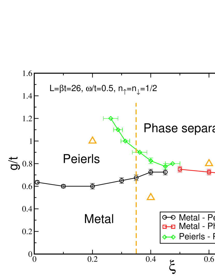
Figure 1: (Color online) Phase diagram for the $U=0$ system as a function of the coupling strength, $g$, and range, $\xi$, of the fermion-phonon coupling. The triangles correspond to three cases which are studied in detail in the text. The dashed line corresponds to the cut shown in Fig. 7.

In Fig. 2, we show the Green functions for the up fermions, $G_{\uparrow}$, and phonons, $G_{\phi}$, as well as fermion density-density correlations, $D_{\uparrow\uparrow}$, in the metallic phase for $\xi=0.4$ and $g/t=0.5$. As expected in a one-dimensional system Giamarchi03 , $G_{\uparrow}$ and $D_{\uparrow\uparrow}$ show an algebraic decay with distance $R$, typical of quasi long range order. Here the dominant effect is the one particle motion, as $G_{\uparrow}$ decays is slower than for $D_{\uparrow\uparrow}$. On the contrary, $G_{\phi}$ shows that the phonons adopt a long range ordered phase. This is expected as the coupling to the fermion density acts as an external field for the phonon displacement, $X_{r}$, and thus provides an explicit symmetry breaking. A simple coherent state approximation shows that, for a homogeneous density of fermions $n$, $\phi=\langle a\rangle=-n\sum_{R}G(R)/\omega$ and $n_{\phi}=G_{\phi}=\phi^{2}$. This simple ansatz yields $G_{\phi}=n_{\phi}=1.12$ for the case considered here, whereas our simulation gives a slightly lower value $G_{\phi}(L/2)=1.016\pm 0.007$. As the number of phonons increases, the coherent state approach describes the system more accurately. For example, for $\xi=g/t=0.6$, it predicts $n_{\phi}=G_{\phi}=1.87$ while the numerical value is $G_{\phi}(L/2)=1.91\pm 0.02$.

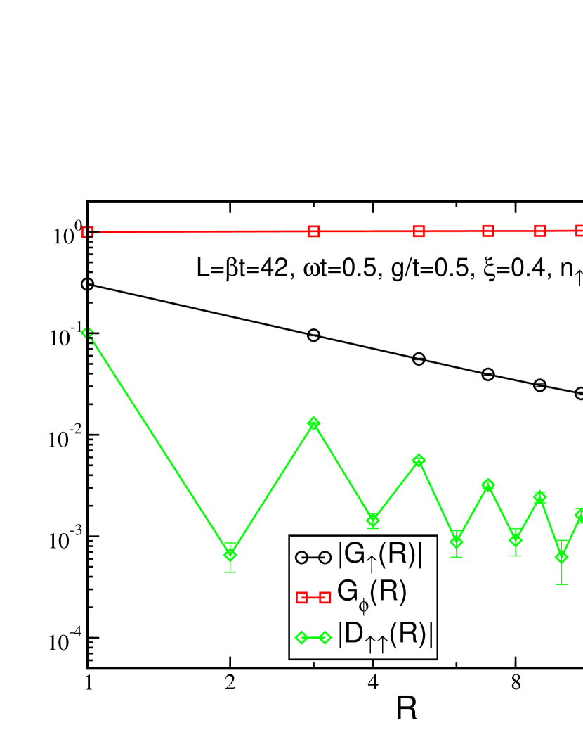
Figure 2: (Color online) The one body Green functions for up fermions, $G_{\uparrow}(R)$, phonons, $G_{\phi}(R)$, and the fermion density-density correlations, $D_{\uparrow\uparrow}(R)$, as functions of distance in the metallic phase. Logarithmic scales are used on both axes. The phonon Green function, $G_{\phi}$, shows long range order while for fermions, $G_{\uparrow}$ and $D_{\uparrow\uparrow}$ show quasi-long range order.

Turning now to the Peierls phase, we observe that, when $g$ is large enough ($\xi=0.2,g/t=1.0$) the homogeneous metallic phase is destabilised and changes into a Peierls state with a modulation of densities (a charge density wave, CDW). All the density-density correlation functions exhibit the same characteristic oscillations with wave vector $k=\pi$ (Fig. 3). Following the previous ansatz, the coupling energy between the fermions and the phonons on a site is roughly proportional to $-n_{r}^{2}g^{2}/\omega$. The electron-phonon coupling energy will then be multiplied by approximately two when the system undergoes a transition from a homogeneous phase where $n_{r}\simeq 1$ on each site to a state where $n_{r}\simeq 2$ every other site. This happens for large enough $g$ as the transition increases the hopping energy: delocalized particles occupy long wavelength states with negative energies, while localized particles have a hopping energy which is approximately zero. The decrease of the coupling energy should then compensate for this hopping energy increase.

The alternation of occupied and empty sites is similar to what is observed in the attractive Hubbard model, with the major difference that the attractive effect between fermions is mediated by the phonon field. The CDW structure is stabilized as it offers the largest amount of virtual hopping possibilities for the fermions.

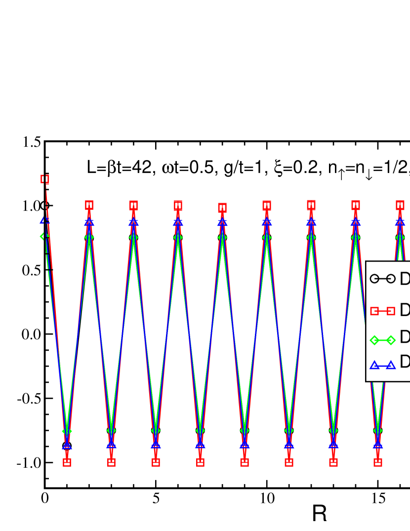
Figure 3: (Color online) Behavior of different density-density correlation functions with distance in the Peierls phase. The Peierls phase shows an alternation of sites that are occupied by fermions and phonons with sites that are almost empty. The functions have been rescaled by respective densities for better visibility.

The localization of the fermions is immediately visible in the behaviour of $G_{\uparrow}(R)$ and $G_{\downarrow}(R)$ which decay exponentially. However, $G_{\phi}(R)$ still shows a plateau at long distances, which shows the condensation of phonons (Fig. 4), albeit modulated by the density wave.

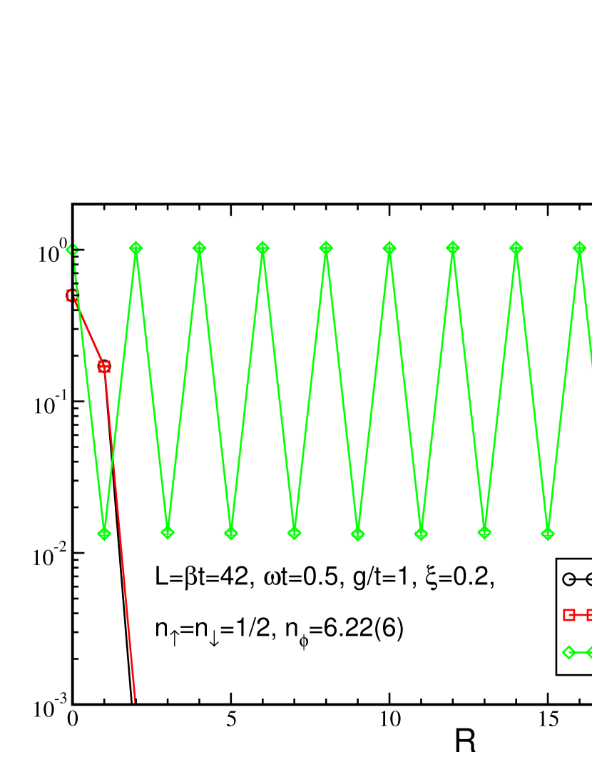
Figure 4: (Color online) Behavior of Green functions in the Peierls phase. The fermion Green functions, $G_{\uparrow}(R)$ and $G_{\downarrow}(R)$, decay rapidly to zero while the phonon Green function, $G_{\phi}(R)$, goes to a plateau when $R$ becomes large. This plateau is modulated by the CDW density oscillations.

Finally, when the range of the coupling is large enough, ($\xi=0.6,g/t=0.8)$, the Peierls phase is destabilized and the system collapses, forming a plateau of fermions and phonons surrounded by empty space (Fig. 5 (a)). This happens as the long range coupling energy overcomes the quantum pressure due to virtual hopping.

The fermionic Green function $G_{\uparrow}(R)$ decays exponentially, as the system is either empty or in a state where the movements of the particles are forbidden by Pauli principle (Fig. 5 (b)). The phonons remain coherent throughout the plateau. $G_{\phi}(R)$ then shows some long range modulations when averaged over all starting sites. If the plateau is located between $r=0$ and $L/2$, $G_{\phi}(R)$ ($R$ positive and smaller than $L/2$) receives non zero contributions from $\langle(a_{r}a^{\dagger}_{r+R}+{\rm H.c.})/2\rangle$ only if both $r$ and $r+R$ are located in the plateau, that is if $0\leq r<L/2-R$. Each non zero contribution is roughly equal to the density of phonons in the plateau. Then $G_{\phi}(R)\propto(L/2-R)/L=1/2-R/L$ decreases linearly with $R$ for $R<L/2$. The same happens for density-density correlation functions, as exemplified by $D_{\uparrow\uparrow}(R)$ (Fig. 5 (b)).

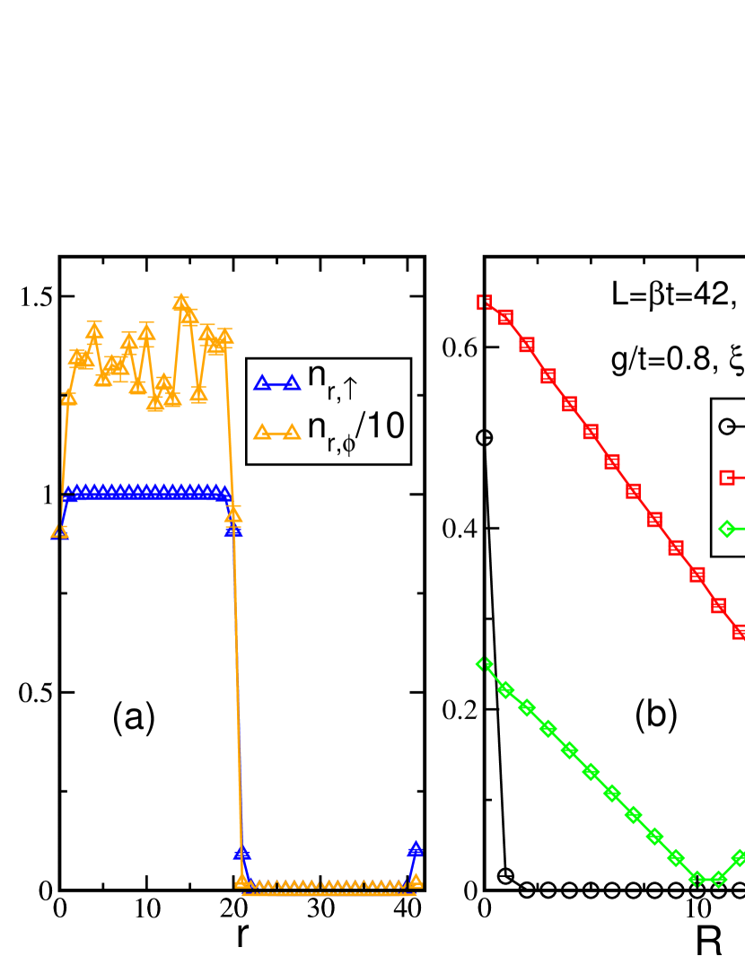
Figure 5: (Color online) (a) For $\xi$ large enough, the fermions and phonons collapse, forming density plateaus in half the system. (b) In that case, the fermionic Green function, $G_{\uparrow}(R)$, decays exponentially to zero while the density-density correlations and phonon Green functions show characteristic long range modulations, due to the plateaus in the density distributions.

We see that, in all three phases, the phonons retain some form of phase coherence, whereas the fermions exhibit quasi-long range coherence only in the metallic phase. In the following we will use the stiffness $\rho_{s,\sigma}$ and the behavior of $G_{\sigma}(R)$ to identify the metallic phase.

To distinguish between the Peierls phase and phase separation, we consider the behaviour of the structure factors (Fig. 6). In all three phases we observe a peak at $k=0$ which simply corresponds to the average density. As expected, in the Peierls phase, $F_{\uparrow\uparrow}(k)$ shows a strong peak at $k=\pi$. The metallic phase shows no particular structure. Finally, the collapsed phase shows a rather irregular form, which is the effect of the frozen plateau observed in Fig. 5. However, the long range modulation induced by the plateau enlarges the $k=0$ peak, which is not observed in the other phases. As such, the value of $F_{\uparrow\uparrow}(k)$ for small values of $k$ is much larger for the collapsed state. Then we can use a large value of $F_{\uparrow\uparrow}(\epsilon)$, where $\epsilon=2\pi/L$, as an indicator that the system has undergone phase separation.

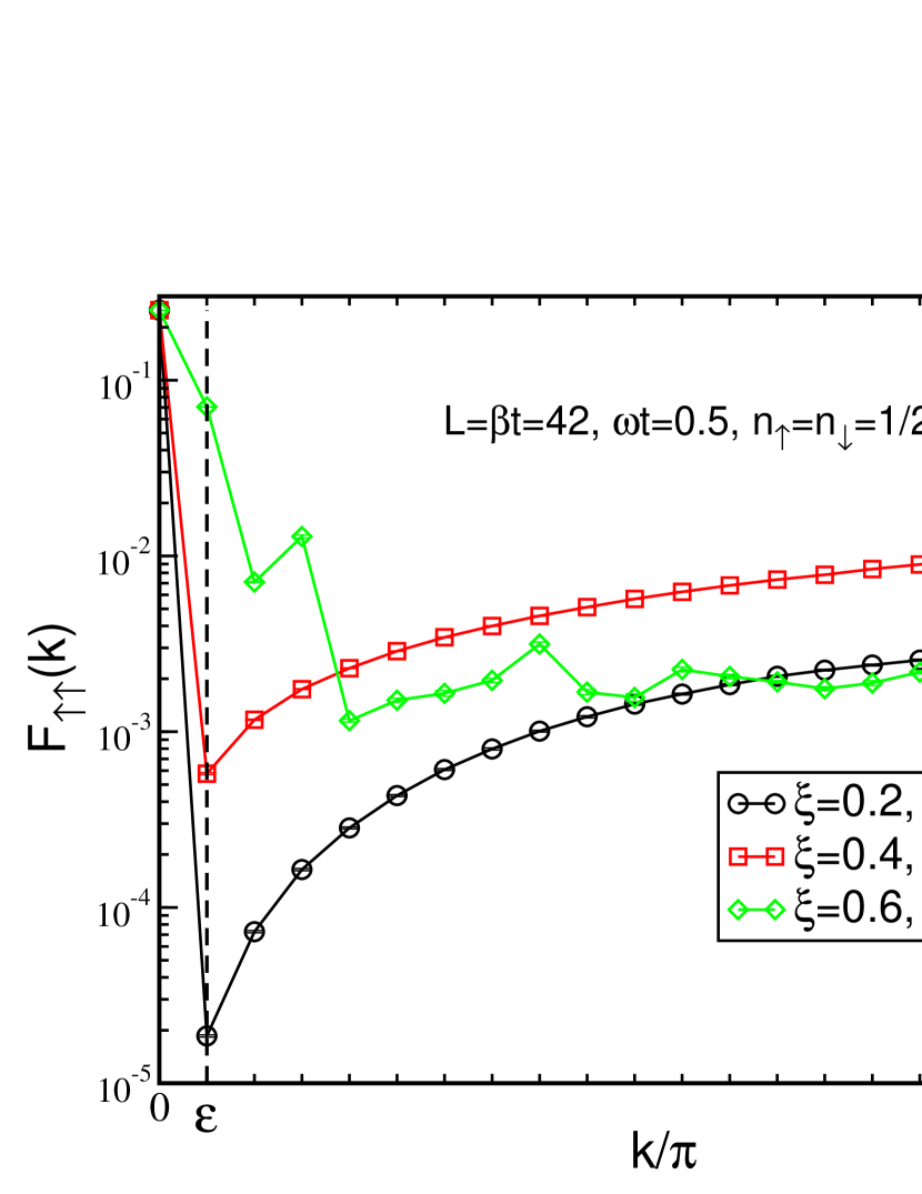
Figure 6: (Color online) Comparison of the behaviour of the structure factor $F_{\uparrow\uparrow}(k)$ in the three phases. In the metallic phase (squares), we only observe a peak at $k=0$ corresponding to the average density. In the Peierls phase (circles), a strong peak appears at $k=\pi$. In the phase separation region (diamond), the peak at $k=0$ is enlarged, giving significantly larger values for $F_{\uparrow\uparrow}(\epsilon)$ where $\epsilon=2\pi/L$.

Using these quantities, we build the phase diagram of the system by doing systematic cuts in the phase space and analyzing the stiffness, $\rho_{s,\uparrow}$, structure factors, $F_{\uparrow\uparrow}(\pi)$ and $F_{\uparrow\uparrow}(\epsilon)$, as well as the phonon density, $n_{\phi}$. We also analyze similar quantities for other types of particles (down fermions, phonons).

A typical cut, for a fixed value of $\xi=0.35$, varying $g/t$, and three sizes $L=26$, 30 and $42$ is shown in Fig. 7. We observe successively the three phases. The metallic phase is characterised by a non zero stiffness $\rho_{s,\uparrow}$. In the metallic phase $F_{\uparrow\uparrow}(\pi)$ takes a small although non zero value as there are quasi long range density-density correlations in this phase. In the Peierls phase, $\rho_{s,\uparrow}$ is zero and $F_{\uparrow\uparrow}(\pi)$ becomes larger as there is true long range order for the density-density correlations. Finally, at large $g$, $F_{\uparrow\uparrow}(\pi)$ becomes suddenly zero while $F_{\uparrow\uparrow}(\epsilon)$ rises. This is accompanied by an abrupt increase of the density of phonons and signals the occurrence of the phase separation. Using these signals, we can plot the phase diagram shown in Fig. 1. It is quite difficult to locate precisely the boundaries of the different regions. As can be observed in Fig. 7, the value of $g$ at which the transition from the Peierls phase to the phase separation regime occurs increases between $L=26$ and $L=30$ and then decreases between $L=30$ and $L=42$, offering no clear systematic scaling behavior.

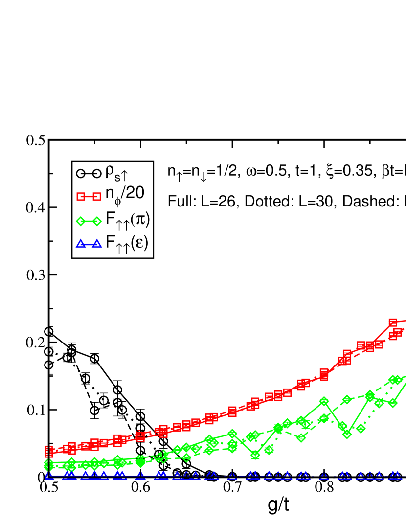
Figure 7: (Color online) The stiffness, $\rho_{s\uparrow}$, phonon density, $n_{\phi}$, and structure factor, $F_{\uparrow\uparrow}$ as functions of $g$ for $\xi=0.35$. We observe three phases: a metallic phase where $\rho_{s,\uparrow}\neq 0$ and $F_{\uparrow\uparrow}(\pi)$ remains small ($g/t\lesssim 0.65$); an intermediate Peierls phase where $\rho_{s,\uparrow}=0$ and $F_{\uparrow\uparrow}(\pi)$ is larger ($0.65\lesssim g/t\lesssim 0.9$); and phase separation, $\rho_{s,\uparrow}=0$, $F_{\uparrow\uparrow}(\pi)=0$ and $F_{\uparrow\uparrow}(\epsilon)\neq 0$ ($0.9\lesssim g/t$). Upon entering the phase separation region, the density of phonons $n_{\phi}$ becomes larger.

At low $\xi$, the simulations are easier to perform and allow a finite size scaling analysis. We identified the transition point $g_{c}$ between the metal and Peierls phases as the point where $\rho_{s,\uparrow}$ reaches half its maximum low $g$ value. Plotting $g_{c}(L)$ as a function of $1/L$ (Fig. 8) we can extrapolate to $L\rightarrow\infty$. For $\xi=0.01\simeq 0$ we find $g_{c}(\infty)/t=0.53\pm 0.03$ which is compatible with previously known results Fehske08 ; Hohenadler12 . For $\xi=0.1$ we find $g_{c}(\infty)/t=0.49\pm 0.02$.

We performed similar analyses with a Langevin algorithmBatrouni19 and found equivalent results (see, for example, Fig. 20 in appendix A).

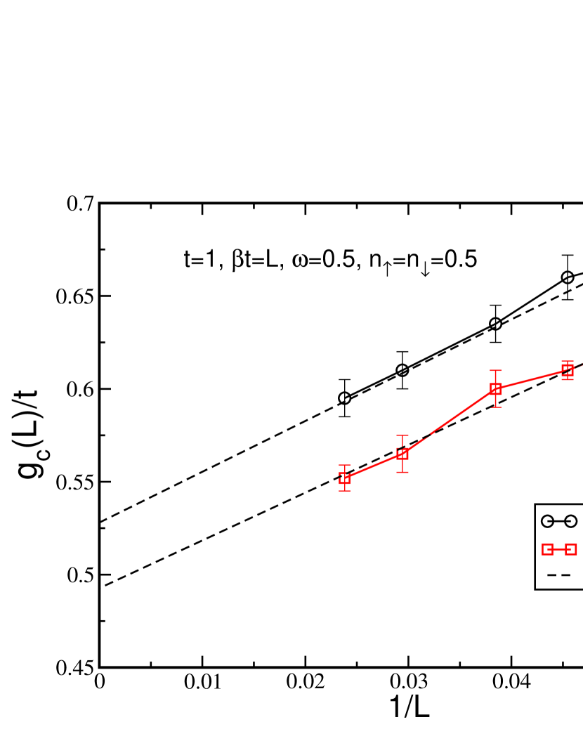
Figure 8: (Color online) Finite size scaling extrapolation of the transition point between the metallic and Peierls phases for low values of $\xi=0.01$ and $\xi=0.1$.

IV Case with non zero electron-electron interaction

We now turn to the case where $U\neq 0$. In addition to the three phases already observed we expect an antiferromagnetic phase to appear in the system at half-filling. We will concentrate on the $g=1$ and $g=0.4$ cases as they correspond to the two typical behaviours observed in the $U=0$ phase diagram (Fig. 1). In the first case, we have a transition from a Peierls to phase separation for $\xi\simeq 0.3$. In the second, we have a metallic phase for all the values of $\xi$ we examined, i.e. up to $\xi=0.8$.

IV.1 $g=1$, half-filled case

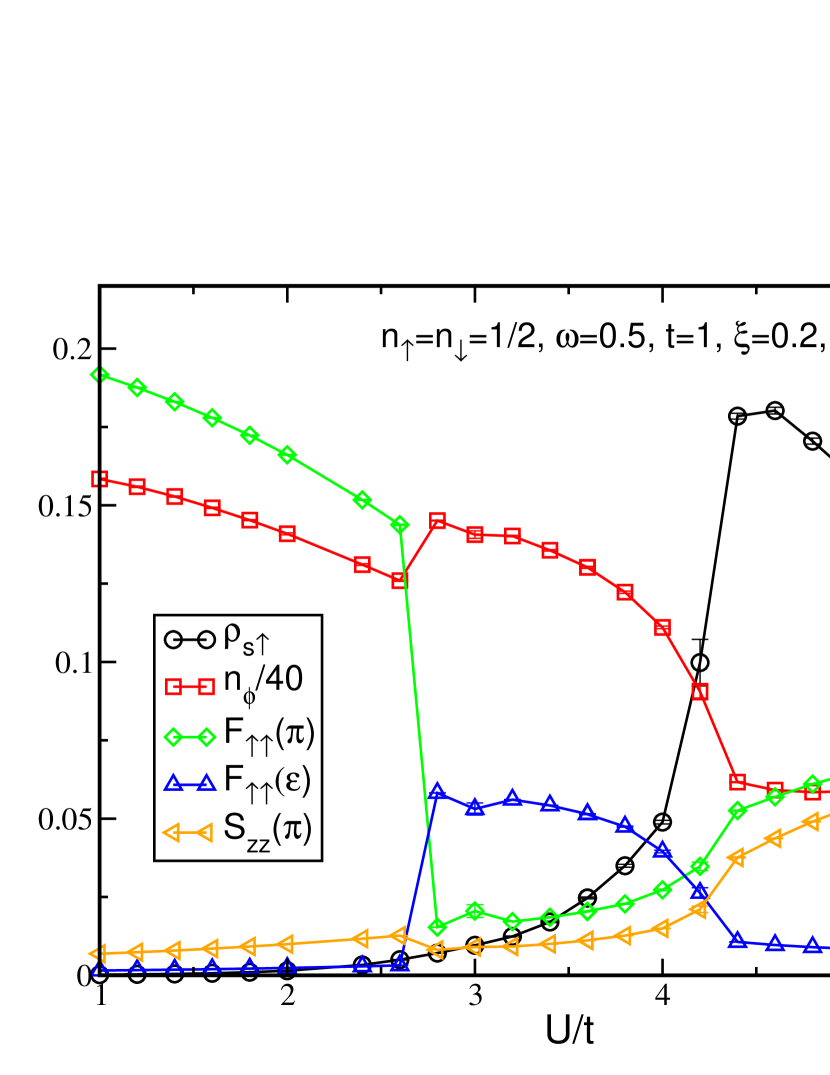
Figure 9: (Color online) Cut in the phase diagram for fixed $g=1$ and $\xi=0.2$. We observe three different phases. At low $U\lesssim 2.8$, the system is in a Peierls phase as the only non zero structure factor is $F_{\uparrow\uparrow}(\pi)$. A phase separated state is found for $2.8\lesssim U\lesssim 4.2$, marked by the larger value of $F_{\uparrow\uparrow}(\epsilon)$. Finally, for $U\gtrsim 4.2$ the system is in an antiferromagnetic state characterized by $S_{zz}(\pi)$, $F_{\uparrow\uparrow}(\pi)$ and $\rho_{s\uparrow}$ being nonzero.

Figure 9 shows the evolution of the system for a fixed $g=1$ and $\xi=0.2$ as $U$ is increased. Starting from a Peierls phase at $U=0$ (Fig. 1), we go through a phase separated state and, finally, an antiferromagnetic Mott phase at large $U$. The presence of the AF phase is demonstrated by the fact that $S_{zz}(\pi)$ is non zero. We also observe that $F_{\uparrow\uparrow}(\pi)$ and the stiffness $\rho_{s,\uparrow}$ are non zero in the AF phase, as expected. The change in behaviour of $n_{\phi}$ also marks the transitions between the different states, as $n_{\phi}$ is generally larger in the collapsed state.

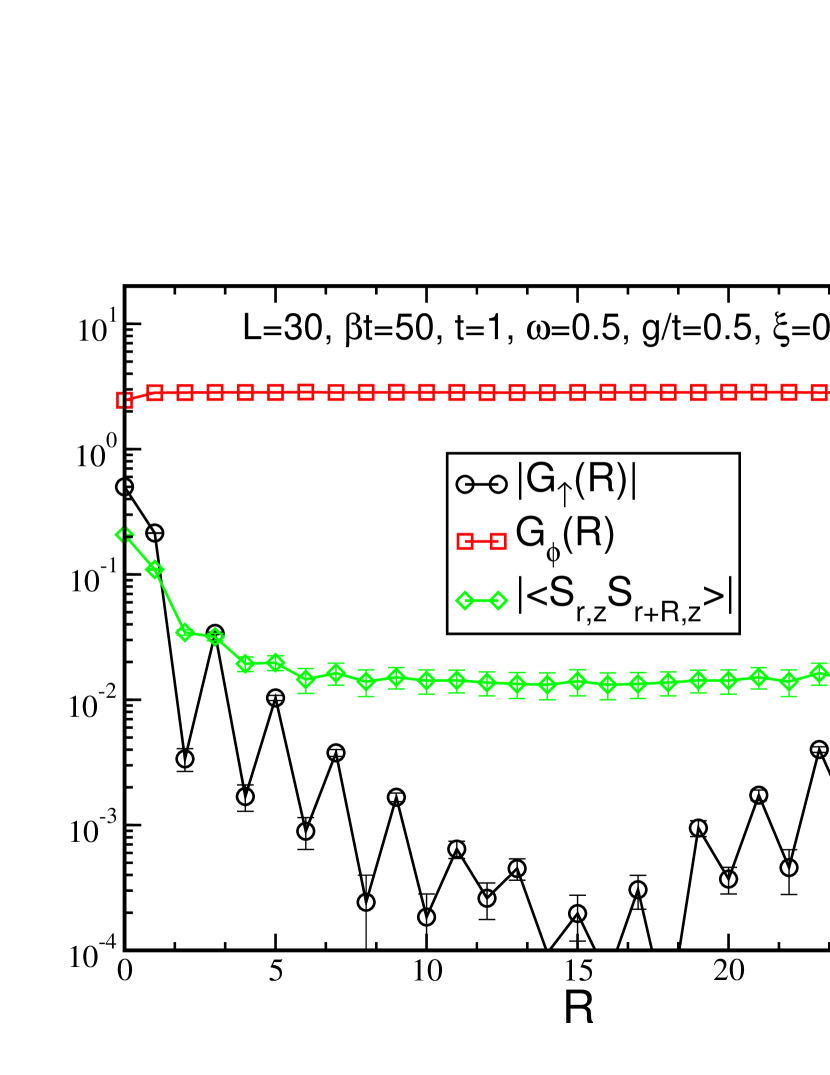
Figure 10: (Color online) Behaviour of correlations as functions of distance $R$ in the antiferromagnetic Mott phase. $G_{\phi}(R)$ shows the long range phase coherence of the phonons. $G_{\uparrow}(R)$ shows the localisation of the individual fermions in the Mott phase. The spin-spin correlations $\langle S_{r,z}S_{r+R,z}\rangle$ decay slowly with a behavior that is compatible with long range or quasi long range orders.

We analyse the AF phase by studying the correlation functions (Fig. 10). As in the other phases, the phonons develop a long range phase coherence shown by the behaviour of $G_{\phi}(R)$. The fermionic Green function $G_{\uparrow}(R)$ decays exponentially with $R$, as expected in a Mott like phase, while the spin-spin correlations $\langle S_{r,z}S_{r+R,z}\rangle$ reach a constant value. In one dimension one would rather expect a quasi long range order with an algebraic decay of $\langle S_{r,z}S_{r+R,z}\rangle$, because of the continuous symmetry of the spin degrees of freedom, but it is not visible here, due to the limited size of the system. A finite size analysis is needed to determine the exact nature of the spin correlations.

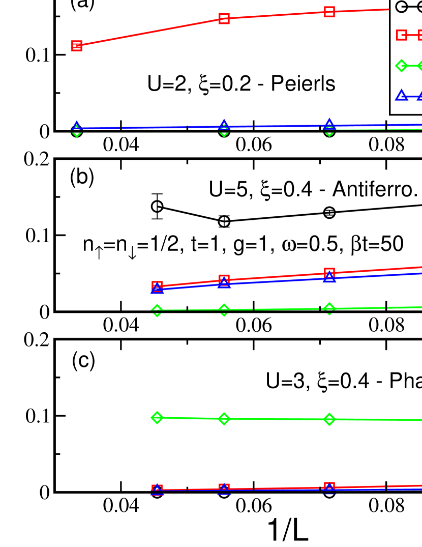
Figure 11: (Color online) Finite size behavior of the structure factors and stiffness in three different regions: Peierls (a), antiferromagnetic (b) and phase separation (c). While in the Peierls and phase separated state cases $F_{\uparrow\uparrow}(\pi)$ and $F_{\uparrow\uparrow}(\epsilon)$, respectively, extrapolates to nonzero values when $L\rightarrow\infty$, $S_{zz}(\pi)$ and $F_{\uparrow\uparrow}(\pi)$ extrapolate to a value compatible with zero in the AF case.

To confirm the presence of three different phases, we perform a finite size analysis (Fig. 11). In the Peierls phase (Fig. 11(a)), $F_{\uparrow\uparrow}(\pi)$ extrapolates to a nonzero value in the large $L$ limit, which signals long range order, while the other structure factors and the stiffness go to zero. The same is true for $F_{\uparrow\uparrow}(\epsilon)$ in the phase separated state (Fig. 11(c)). In contrast, in the AF phase (Fig. 11(b)) the leading structure factors $S_{zz}(\pi)$ and $F_{\uparrow\uparrow}(\pi)$ decrease with size. A linear fit gives a value in the $L\rightarrow\infty$ limit that is compatible with zero. At the same time, the stiffness $\rho_{s,\uparrow}$ extrapolates to a non zero value. This is characteristic of the quasi-long-range AF order that one expects in one dimension.

Using cuts similar to Fig. 9 for three different sizes, $L=10,14$, and $18$, at $\beta t=50$, we draw the phase diagram for $g=0.1$ in the $(\xi,U)$ plane at half-filling (Fig. 12). We find the three phases presented before. The phase separated region extends between the Peierls and AF phase, down to $\xi\simeq 0.1$. To confirm the presence of a direct Peierls AF transition at low $\xi$ we performed simulations at fixed small values of $\xi=0,0.025$ and 0.05 (Fig. 13). In all these cases, we found that $F_{\uparrow\uparrow}(\epsilon)$ always remains zero, indicating that there is no phase separation and indeed a direct transition from the Peierls phase to the AF phase. In the $\xi=0$ limit, our system is the conventional Hubbard-Holstein model. We observe a transition from the Peierls to the Mott insulator for $U\simeq 5.4$ but in this regime, we are limited to small sizes ($L$ up to 18 only). Previous studies Hardikar07 ; Fehske08 ; Tezuka07 located this transition at a lower value, slightly above $U=4$. For larger values of $\omega$, there may be an intermediate metallic phase but this is not the case for $\omega=t/2$.Hardikar07 ; Fehske08 ; Tezuka07

To locate better the left boundary of the phase separation region, we did some simulations with parameters $U$ and $\xi$ chosen along diagonal lines in the phase diagram (see the dotted dashed line in Fig. 12) as shown in Fig. 14. We again note an absence of phase separation for $\xi\lesssim 0.1$. As in the $U=0$ case, the phase separation does not seem to persist down to $\xi=0$. This is not surprising as the range needs to be long enough to collapse the system.

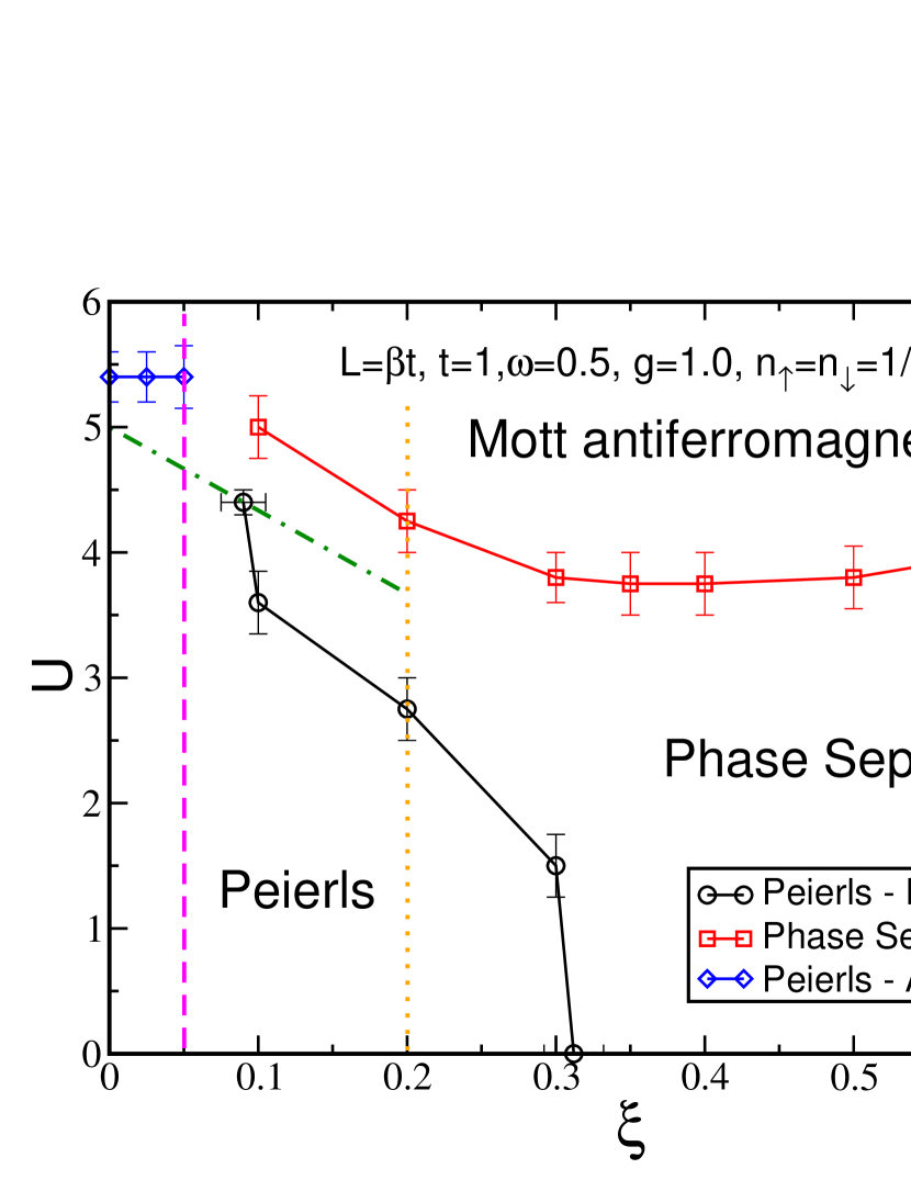
Figure 12: (Color online) Phase diagram for $g=1$ and $\omega=0.5$ in the half-filled case in the $(\xi,U)$ plane. We observe three phases, a Peierls phase at low $U$ and $\xi$, phase separation at low $U$ and large $\xi$ and an AF Mott insulator state at large $U$. The dotted line corresponds to the cut shown in Fig. 9, the dashed line to Fig. 13, and the dotted dashed line to Fig. 14.

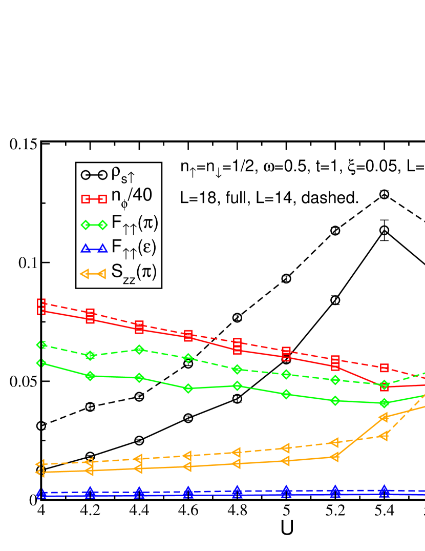
Figure 13: (Color online) Cut in the phase diagram at small $\xi=0.05$ to observe the direct transition from Peierls to AF. $F_{\uparrow\uparrow}(\epsilon)$ always remains zero and there is no sign of a phase separation. The transition from Peierls to AF is difficult to observe but is visible in the small jump in the value of $S_{zz}(\pi)$.

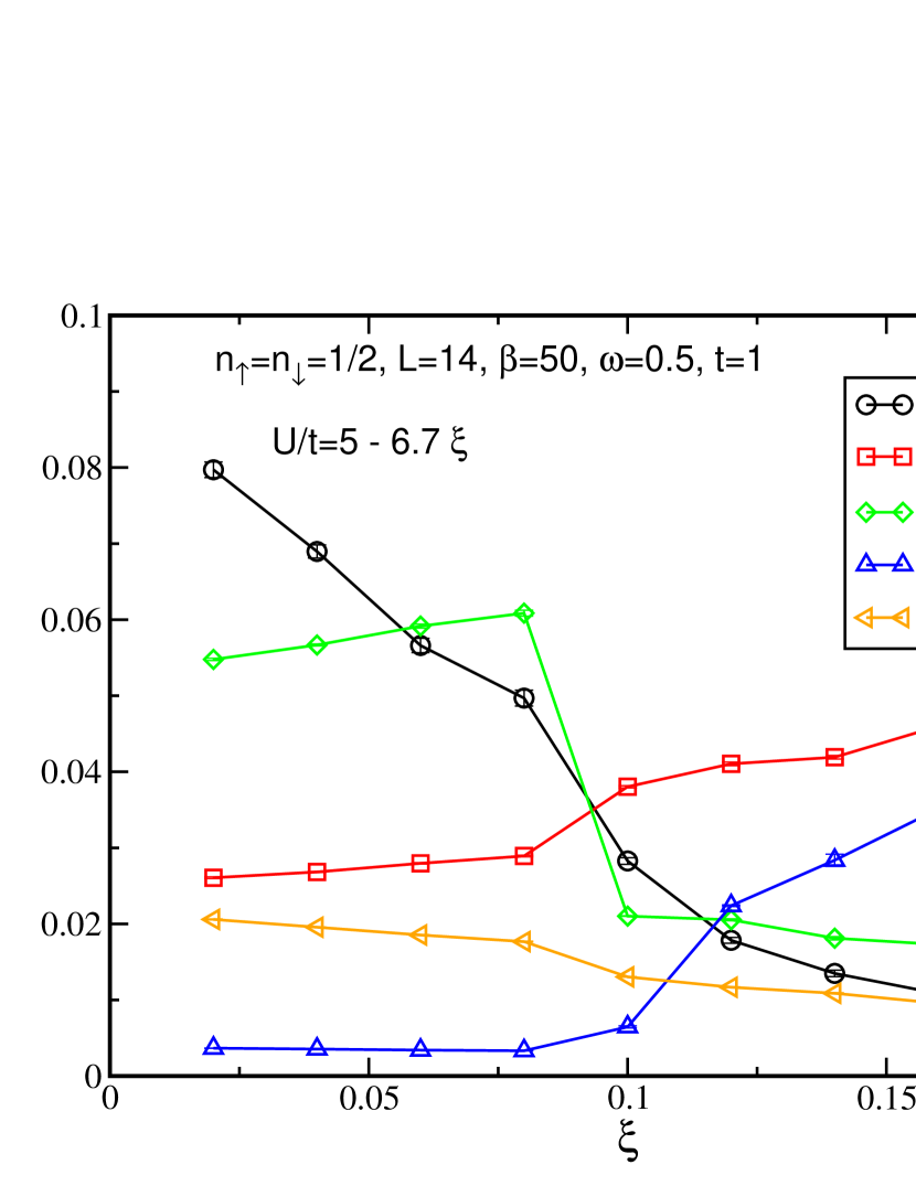
Figure 14: (Color online) Cut in the phase diagram along the dotted dashed diagonal line in Fig. 12 where $U/t=5-6.7\,\xi$. We observe a transition from Peierls to phase separation. For $\xi\lesssim 0.1$, $F_{\uparrow\uparrow}(\epsilon)$ is negligible while $F_{\uparrow\uparrow}(\pi)$ is large, which signals the Peierls phase. For $\xi\gtrsim 0.1$, $F_{\uparrow\uparrow}(\epsilon)$ becomes non zero and marks the entry into the phase separated region.

IV.2 $g=0.4$, half-filled case

For a lower value, $g=0.4$, the situation is simpler. As observed in the $U=0$ case, for low $g$, the system does not show phase separation. When electron-electron interactions are increased the system then simply undergoes a transition from a metallic state to a Mott antiferromagnet.

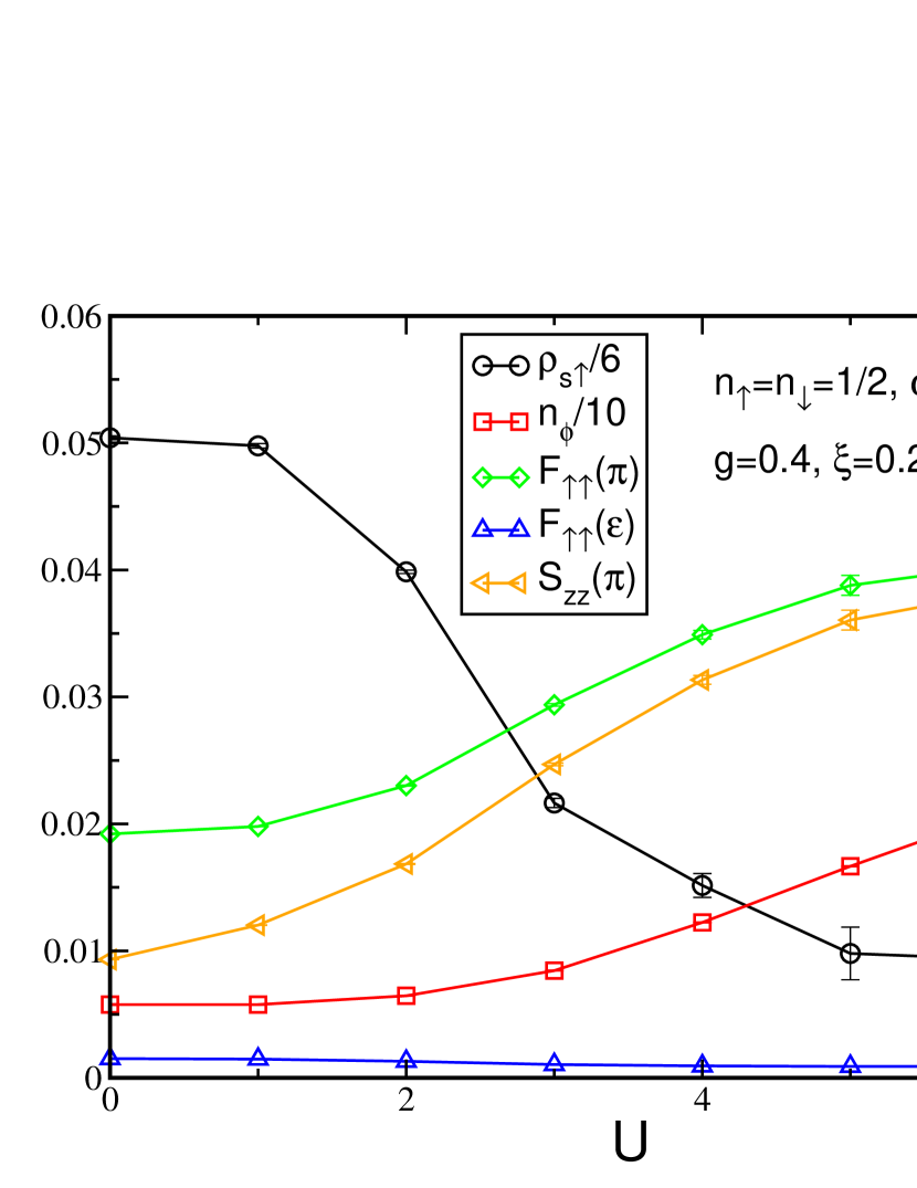
Figure 15: (Color online) Structure factors, density of phonons, $n_{\phi}$, and stiffness, $\rho_{s,\uparrow}$, as functions of $U$ for $g=0.4$. The system goes from a metallic to an AF phase as $U$ is increased without experiencing phase separation.

This is first observed in the evolution of the structure factors in Fig. 15: As $U$ increases, so do $S_{zz}(R)$ and $F_{\uparrow\uparrow}(\pi)$. In contrast, the stiffness $\rho_{s\uparrow}$, while nonzero in both the metallic and AF phases, drops when one enters the second.

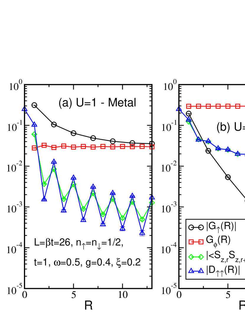
Figure 16: (Color online) Correlations as functions of distance for $g=0.4$ and $\xi=0.2$ in the metallic phase at low $U=1$ (a) and in the antiferromagnetic phase at $U=6$ (b).

It is a bit difficult to distinguish the AF phase from the metallic one in one dimension. Indeed, we do not expect long range magnetic order for the AF phase and, in one dimension, the metallic phase should be described by Luttinger physics and also shows some quasi long range order for the density and spin correlations.

This is indeed what is observed in Fig. 16 which shows different correlation functions for weak ($U=1$) and strong ($U=6$) interactions (Fig. 16 (a) and (b), respectively). For $U=1$, we observe quasi long range order for the fermion Green function $G_{\uparrow}(R)$, the spin-spin correlation $\langle S_{z,r}S_{z,r+R}\rangle$, and the density-density correlation $D_{\uparrow\uparrow}(R)$, although the fermion Green function is clearly the leading correlation in that case. We also observe, as mentioned before, a true long range order for the phonon phase coherence $G_{\phi}(R)$.

On the contrary, for $U=6$ (Fig. 16(b)), we observe that the spin-spin and density-density correlations remain quasi long ranged while the fermionic Green function decays exponentially, which is the sign that we are in a Mott insulating phase. This time, the leading effects are clearly spin correlations. The phonons still show long range phase order.

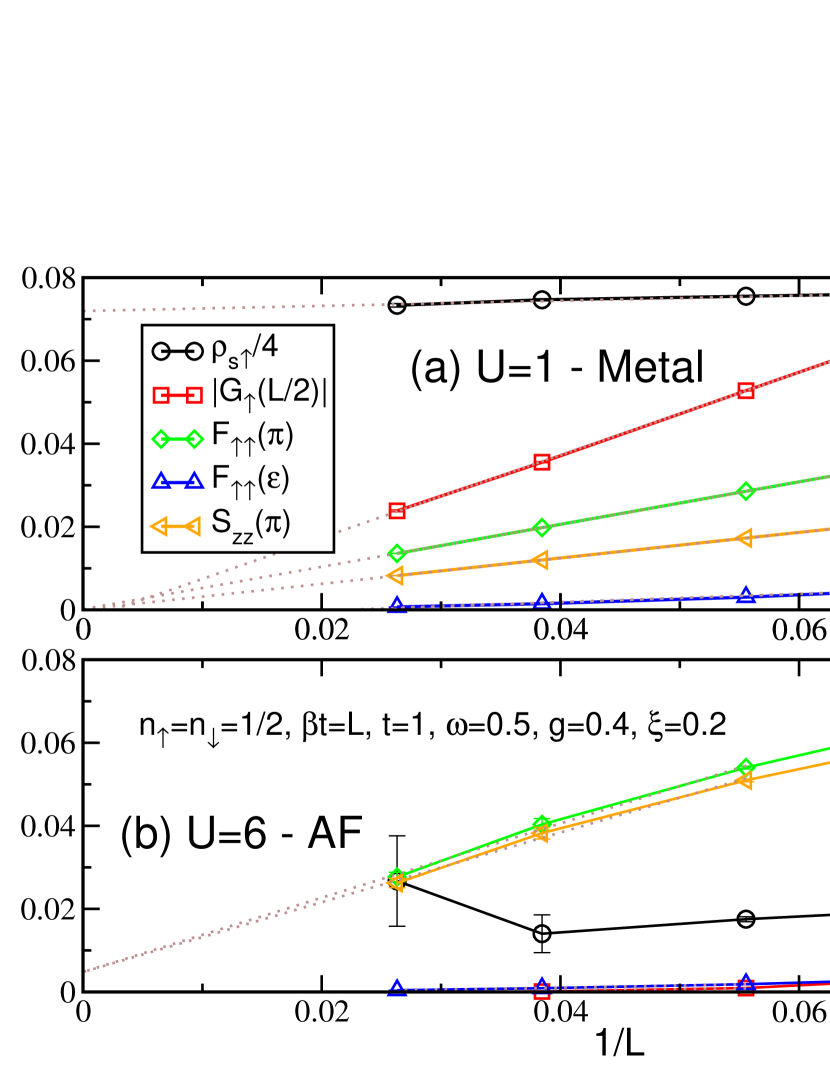
Figure 17: (Color online) Scaling of different quantities with size $L$ for $g=0.4$ and $\xi=0.2$ in the metallic phase at low $U=1$ (a) and in the antiferromagnetic phase at $U=6$ (b). In both, all quantities extrapolate to zero except for the stiffness $\rho_{s\uparrow}$. In the metal (a), the one body Green function $G_{\uparrow}(R)$ is the leading correlation, whereas in the AF (b), $S_{zz}(\pi)$ and $F_{\uparrow\uparrow}(\pi)$ are the leading correlations. The stiffness is difficult to measure in this second case.

Looking at the scaling of these quantities as a function of size $L$ in the metal $U=1$ phase (Fig. 17(a)) and AF phase (Fig. 17(b)) we observe that all quantities scale to zero, except for the stiffness. This was expected for a one dimensional system, as all correlation functions show at most quasi long range order. In the metallic phase, we observe a sizeable one particle Green function at long distances $G_{\uparrow}(L/2)$ as well as noticeable spin-spin $S_{zz}(\pi)$ and density correlations $F_{\uparrow\uparrow}(\pi)$. In the AF phase, $S_{zz}(\pi)$ and $F_{\uparrow\uparrow}(\pi)$ become the leading correlations while $G_{\uparrow}(L/2)$ is exponentially suppressed in that case.

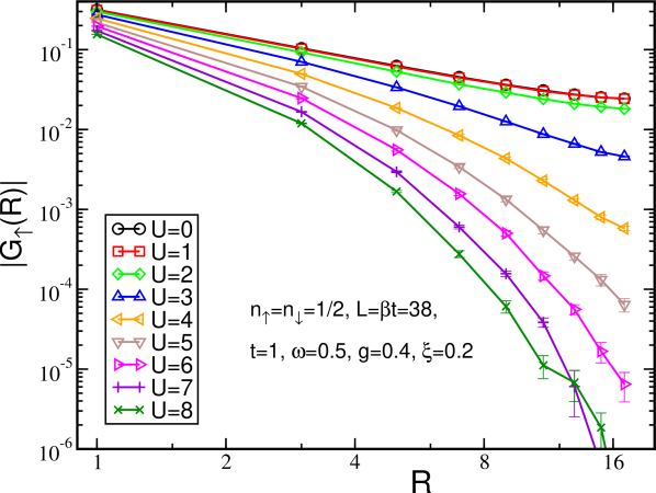
Figure 18: (Color online) Behavior of the one particle Green function $G_{\uparrow}(R)$ for $g=0.4$ and $\xi=0.2$ and different values of $U$. The behavior changes from an algebraic decay for $U\lesssim 4$ to an exponential one for $U\gtrsim 4$.

As we do not have true long range order in these two phases, the only behavior that allows their identification is that of the correlation functions, especially $G_{\uparrow}(R)$ that changes from an algebraic to an exponential decay (Fig. 18). Examining simulations on a $L=38$ system, we find a transition around $U\simeq 4$ for $g=0.4$ and $\xi=0.2$. This, unsurprisingly, corresponds to the point where the stiffness $\rho_{s\uparrow}$ drops in Fig. 15.

Finally $F_{\uparrow\uparrow}(\epsilon)$ decays rapidly to zero in both cases, which shows that there is no tendency towards phase separation for $g=0.4$.

V Summary

We studied a one-dimensional Hubbard-Holstein model with long range coupling between fermions and phonon, and on-site interaction between fermions. The results presented here are limited to the case of phonon frequency $\omega=t/2$. The physics of the Hubbard-Holstein with on-site phonon coupling for larger values of $\omega$ has been studied inHardikar07 ; Fehske08 ; Tezuka07 .

For $U=0$, the Holstein model, we observed, at half-filling, three different phases: A metal at low $g$ and, for larger $g$, a transition from a Peierls CDW phase at small coupling range $\xi$ to a phase separation region for larger values of $\xi$ (Fig. 1). This is reminiscent of the results found in a previous study Hohenadler12 although we found the phase separation region to extend to much smaller values of $\xi$.

Introducing strong enough electron-electron interactions, $U$, drives the half-filled system towards a Mott antiferromagnetic phase. For large $g=1$, the Peierls phase or phase separated region will transform into a Mott for $U\simeq 5$. However, we observe, as in the non $U=0$ case, that the phase separation region extends to low $\xi\simeq 0.1$, coming in between the Peierls and Mott phases (Fig. 12). A direct Peierls-Mott transition is observed only for small values of $\xi$. For $g=0.4$, the metallic phase present for all studied values of $\xi$ is transformed into an AF Mott phase without an intermediate phase (Fig. 15).

Appendix A Numerical methods

A.1 Stochastic Green function (SGF) algorithm

The SGF algorithm, introduced in Refs. Rousseau08-1, ; Rousseau08, , is a quantum Monte Carlo algorithm which evolved from the Worm Proko98 and canonical Worm algorithmsVanHoucke06 . The main interest of the SGF algorithm is to allow the measurement of $n$ points equal time Green functions and the simulation of complex models, especially models that do not conserve the number of particles.

If the Hamiltonian is written as the sum of two parts $H=V-K$, where $V$ is diagonal (in a chosen basis) and $K$ nondiagonal, the partition function can then be expressed as an expansion in powers of $K$ Proko98

$$Z={\rm Tr}\sum_{n=0}^{\infty}\int_{0<\tau_{1}<\tau_{2}\cdots<\tau_{n}<\beta}d\tau_{1}\cdots d\tau_{n}\ \ e^{-\beta V}K(\tau_{n})\cdots K(\tau_{1}),$$ (6)

where $K(\tau)=e^{\tau V}Ke^{-\tau V}$. Here we will choose the occupation number basis. We then have $V=U\sum_{r}n_{r,\uparrow}n_{r,\downarrow}+\omega\sum_{r}n_{r,\phi}$ and $K=t\sum_{r,\sigma}c_{r,\sigma}^{\dagger}(c_{r+1,\sigma}^{\phantom{\dagger}}+{\rm H.c.})-\sum_{r,R}G(R)\sqrt{2}X_{r}n_{r+R}$.

Introducing complete sets of states $|\psi_{\tau}\rangle$ between nondiagonal operators, we obtain

$$Z = \sum_{n=0}^{\infty}\sum_{\{|\psi_{\tau}\rangle\}}\int_{0<\tau_{1}<\tau_{2}\cdots<\tau_{n}<\beta}d\tau_{1}\cdots d\tau_{n}\ \ \langle\psi_{0}|e^{-\beta V}K(\tau_{n})|\psi_{n-1}\rangle$$

$$\times\langle\psi_{n-1}|K(\tau_{n-1})|\psi_{n-2}\rangle\langle\psi_{n-2}|K(\tau_{n-2})|\psi_{n-3}\rangle\cdots$$

$$\times\langle\psi_{2}|K(\tau_{2})|\psi_{1}\rangle\langle\psi_{1}|K(\tau_{1})|\psi_{0}\rangle.$$

If the product of the matrix elements of the form $\langle\psi_{k}|K(\tau_{k})|\psi_{k-1}\rangle$ is positive, it can be used as a weight with which to sample all the variables ($\{\tau_{k}\}$, $\{|\psi_{k}\rangle\}$ and the expansion order $n$). In practice, we resort to the Jordan-Wigner mapping of fermions onto hardcore bosons to simulate this one-dimensional fermionic system and avoid a sign problem for the weight.

In order to sample $Z$, an extended partition function is introduced $Z(\tau)={\rm Tr}e^{-(\beta-\tau)H}{\mathcal{G}}e^{-\tau H}$ where $\mathcal{G}$ is the Green operator defined by

$${\mathcal{G}}=\sum_{p,q=0}^{\infty}w_{pq}\sum_{\{c_{k}|d_{l}\}}\prod_{k=1}^{p}\frac{b^{\dagger}_{c_{k}}}{\sqrt{n_{c_{k}}+1}}\prod_{l=1}^{q}\frac{b_{d_{l}}}{\sqrt{n_{d_{l}}+1}}.$$ (7)

Here the $b^{\dagger}_{c}$ operator creates a particle in state $c$. State $c$ is specified by the type of particle that is created (in our case, two kinds of hardcore bosons, representing spin up and spin down fermions, or phonons) and by the site on which it is created. The $b_{d}$ operator destroys a particle in state $d$, in the same way. In the Green operator, the $c$ and $d$ states should be different, so that there are no diagonal contributions in the Green operator, except for $q=p=0$ which gives the identity operator. As the terms in $\mathcal{G}$ are products of creation and destruction operators, $\mathcal{G}$ is then the sum of all possible $n$-point Green functions, weighted by the matrix $w_{pq}$. The Green functions that have large weights $w_{pq}$ will appear more often is the sampling of $Z(\tau)$.

$Z(\tau)$ is expressed in the same way as $Z$, introducing an additional set of complete states,

$$Z(\tau) = \sum_{n=0}^{\infty}\sum_{\{|\psi_{\tau}\rangle\}}\int_{0<\tau_{1}<\tau_{2}\cdots<\tau_{n}<\beta}d\tau_{1}\cdots d\tau_{n}\ \ \langle\psi_{0}|e^{-\beta V}K(\tau_{n})|\psi_{n-1}\rangle$$ (8)

$$\times\cdots\times\langle\psi_{L+1}|K(\tau_{L})|\psi_{L}\rangle\times\langle\psi_{L}|{\mathcal{G}}(\tau)|\psi_{R}\rangle$$

$$\times\langle\psi_{R}|K(\tau_{R})|\psi_{R-1}\rangle\times\cdots\times\langle\psi_{1}|K(\tau_{1})|\psi_{0}\rangle,$$

where we used labels $L$ and $R$ to denote the states appearing on the left and right of $\mathcal{G}$.

Whenever $|\psi_{L}\rangle=|\psi_{R}\rangle$ during the sampling, the contribution of the Green operator is the simple constant $w_{00}$. The configuration that is then obtained by sampling $Z(\tau)$ also contributes to the original partition function $Z$. When $|\psi_{L}\rangle\neq|\psi_{R}\rangle$, only one of the terms present in $\mathcal{G}$ gives a non zero contribution to $\langle\psi_{L}|{\mathcal{G}}|\psi_{R}\rangle$. In that case, the configuration obtained contributes to the sampling of one peculiar Green function.

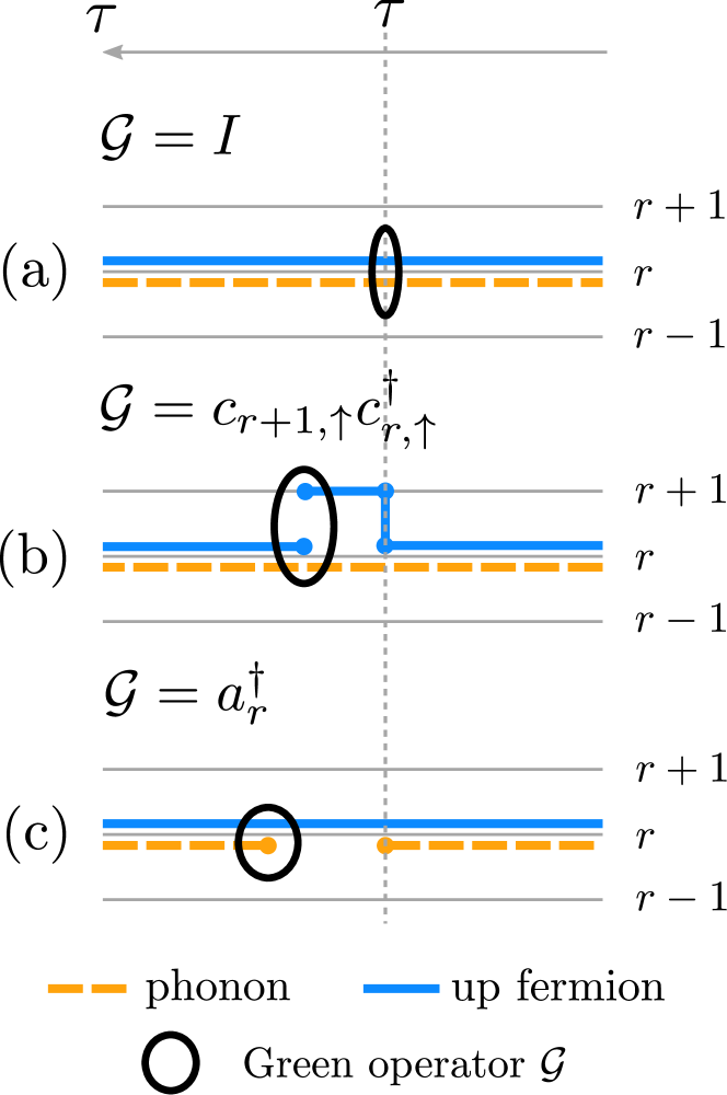
Figure 19: (Color online) Schematic representation of the movement of the Green operator ${\mathcal{G}}$. Starting from an initial configuration (a) where ${\mathcal{G}}=I$ and where there is one up particle (blue thick line) and a phonon (orange thick dashed line) on site $r$, $\mathcal{G}$ is shifted to the left ($\tau$ increasing) and a $K$ operator is created. In (b), a jump of the particle has been created, which modified the state on the right of $\mathcal{G}$ and the $\mathcal{G}$ operator itself. In (c) a destruction operator for the phonon has been created and $\mathcal{G}$ is a phonon creation operator.

In practice, the sampling of the extended partition function is made by using the Green operator. In the simplified update scheme introduced in Rousseau08 , two possible “movements” of $\mathcal{G}$ are shown to allow an ergodic sampling of the configurations. First a shift direction is chosen for ${\mathcal{G}}(\tau)$ (left if $\tau$ is increased, right if $\tau$ is decreased). Then moving in this direction, two different situations can occur: the Green operator can create a $K$ operator at its imaginary time and then be shifted, or the Green operator can be shifted to the imaginary time of the next $K$ operator and destroy it. Creating a $K$ operator requires to choose a new $|\psi_{R}\rangle$ state, assuming that a left move is chosen. Depending on the chosen $|\psi_{R}\rangle$, the Green operator is modified accordingly and only one of the terms appearing in $K$ gives a non zero contribution. The choice between all possible new $|\psi_{R}\rangle$ is made with a probability chosen to respect detailed balance. For example, in our case, the $K$ operator comprises two kinds of operators: jumps of particles from one site to the next or creation or destruction of a phonon. The creation of such operators and the corresponding modifications of the states and Green operator are illustrated in Fig. 19. The destruction of a $K$ operator modifies in the same way $\mathcal{G}$ and the states.

The Green operator is moved until it becomes the identity operator, at which point the measurement of diagonal quantities can be performed. To sample efficiently $Z(\tau)$, a directed propagation Rousseau08 is generally used to avoid $\mathcal{G}$ going back and forth in imaginary time. In that case, there is a stronger probability for the operator to continue its movement in the same direction as in the previous step.

A.2 Langevin algorithm

The Langevin method we used is introduced and benchmarked in Batrouni19 where some additional results for $U=0$ are also presented.

The method initially proceeds in a way that is similar to a determinant quantum Monte Carlo method dqmc (DQMC). We first rewrite the phonon diagonal energy of Hamiltonian (1) as $\omega n_{r,\phi}=\omega x_{r}^{2}/2+p_{r}^{2}/2$ and add a chemical potential term $-\mu\sum_{r}n_{r}$ to the Hamiltonian as the algorithm works in the grand canonical ensemble. When $\mu=-[\sum_{R}G(R)]^{2}/\omega$, the resulting Hamiltonian is particle-hole symmetric and $\langle n_{\uparrow}\rangle=\langle n_{\downarrow}\rangle=1/2$.

The partition function is written as a discrete path integral, where inverse temperature $\beta$ is divided into $L_{\tau}$ steps of size $\Delta\tau=\beta/L_{\tau}$ and complete sets of states $\{x_{r,\tau},p_{r,\tau}\}$ are introduced at each imaginary time step $\tau$. When $U=0$, the fermionic terms in the Hamiltonian (1) are quadratic and can be traced out, and the momentum dependence of the phonons can be integrated out, leading to an expression of the partition function that depends only on the phonon field $x_{r,\tau}$ Scalettar89

$$Z = \int\mathcal{D}x_{r,\tau}\exp(-S_{\rm Bose}(\{x_{r,\tau}\}))[\det M(\{x_{r,\tau}\})]^{2}$$ (9)

$$= \int\mathcal{D}x_{r,\tau}\exp(-S(\{x_{r,\tau}\})).$$

Detailed expressions for $S_{\rm Bose}$ and matrix $M$ are found in Batrouni19 ; dqmc . $M$ is a large sparse matrix of dimension $LL_{\tau}$ and the method is free of the sign problem as the determinant of $M$ is squared.

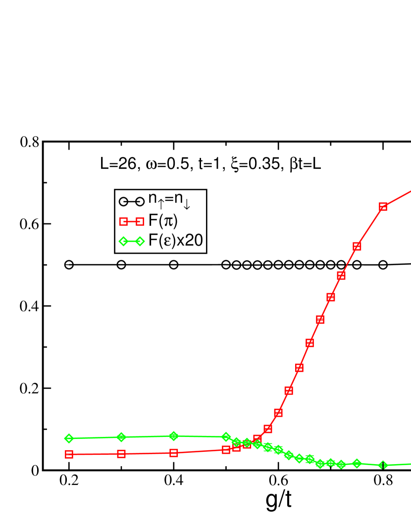
Figure 20: (Color online) Langevin simulations results for a cut in the phase diagram using the same parameters as in Fig. 7. Chemical potential is set to $\mu=-[\sum_{R}G(R)]^{2}/\omega$ to impose particle hole symmetry. $F(k)$ is the Fourier transform of $\langle n_{r}n_{r+R}\rangle$. We observe a homogeneous metallic phase for $g/t\lesssim 0.6$ where the density structure factors are small. A Peierls phase is observed for $0.6\lesssim g/t\lesssim 0.9$, marked by a large value of $F(\pi)$. Finally a phase separated region is obtained for $g/t\gtrsim 0.9$ as shown by the increase of $F(\epsilon)$ and by the average densities $\langle n_{\uparrow}\rangle=\langle n_{\downarrow}\rangle$ that are no longer 1/2.

The algorithm then proceeds by using a fictitious stochastic dynamics, governed by the Langevin equation

$$\frac{dx_{r,\tau}(t)}{dt}=-\frac{\partial S}{\partial x_{r,\tau}(t)}+\sqrt{2}\eta_{r,\tau}(t),$$ (10)

where $\eta_{r,\tau}(t)$ are stochastic variables satisfying

$$\langle\eta_{r,\tau}(t)\rangle=0,\ \langle\eta_{r,\tau}(t)\eta_{r^{\prime},\tau^{\prime}}(t^{\prime})\rangle=\delta_{r,r^{\prime}}\delta_{\tau,\tau^{\prime}}\delta(t-t^{\prime}).$$

The Langevin dynamics assures that, when $t\rightarrow\infty$, variables are distributed according to $P=\exp(-S)$.

Two main technical difficulties need to be overcome in order to integrate the Langevin equations efficiently. First, calculating $\partial S/\partial x_{r,\tau}(t)$ involves Batrouni19 a trace over an expression containing the inverse of matrix $M$. This would be extremely taxing in terms of simulation time, as inverting a matrix scales as the cube of its dimension. This trace is then calculated using a stochastic estimator which allows to replace the matrix inversion problem with a much simpler solution of a linear system. This solution is obtained by a conjudate gradient method that scales linearly with the dimension of $M$, $LL_{\tau}$. This is a big advantage of this method as other techniques, such as the conventional DQMC algorithm, scale as $L^{3}L_{\tau}$. The second difficulty comes from the autocorrelation times of the Langevin dynamics, which are generally very long. This is solved by the so-called Fourier acceleration of the Langevin dynamicsBatrouni19 .

A.3 Langevin simulations results

Using this algorithm, we confirmed the results obtained with the SGF algorithm at $U=0$, especially the fact that a phase separation is present for small values of $\xi$. Fig. 20 shows a cut in the phase diagram for the same parameters as in Fig. 7. As with SGF simulations, we observe a transition from the metal to the Peierls phase for $g/t\simeq 0.6$ and from the Peierls phase to a phase separated behavior for $g/t\simeq 0.9$. The Peierls phase is here signalled by the large value of $F(\pi)$ in the intermediate region, where $F(k)$ is the Fourier transform of $\langle n_{r}n_{r+R}\rangle$. The phase separation is marked by the increased value of $F(\epsilon)$ and, because the simulations are performed in the grand canonical ensemble, by the fact that the densities $\langle n_{\uparrow}\rangle=\langle n_{\downarrow}\rangle$ departs from their expected value of 1/2. Indeed, the density of particles in the system becomes arbitrary in the phase separation region despite the fact that the chemical potential has been chosen to ensure particle hole symmetry.

References

- (1) H. Fröhlich, Adv. Phys. 3, 325 (1954).
- (2) L. N. Cooper, Phys. Rev. 104, 1189 (1956).
- (3) R. Peierls, Surprises in Theoretical Physics, Princeton University Press (1979).
- (4) T. Holstein, Ann. Phys. 8, 325 (1959).
- (5) R.T. Scalettar, N.E. Bickers, and D.J. Scalapino, Phys. Rev. B 40, 197 (1989).
- (6) F. Marsiglio, Phys. Rev. B 42, 2416 (1990).
- (7) Ross H. McKenzie, C. J. Hamer, and D. W. Murray, Phys. Rev. B 53, 9676 (1996).
- (8) J. K. Freericks, M. Jarrell, and D. J. Scalapino, Phys. Rev. B 48, 6302 (1993).
- (9) Robert J. Bursill, Ross H. McKenzie, and Chris J. Hamer, Phys. Rev. Lett. 80, 5607 (1998).
- (10) E. Jeckelmann, C. Zhang, and S.R. White, Phys. Rev. B 60, 7950 (1999).
- (11) J.E. Hirsch and E. Fradkin, Phys. Rev. Lett. 49, 402 (1982).
- (12) J.E. Hirsch and E. Fradkin, Phys. Rev. B 27, 4302 (1983).
- (13) J. Greitemann, S. Hesselmann, S. Wessel, F.F. Assaad, and M. Hohenadler, Phys. Rev. B 92, 245132 (2015).
- (14) R.P. Hardikar and R.T. Clay, Phys. Rev. B 75, 245103 (2007).
- (15) J.T. Devreese and A.S. Alexandrov, Rep. Prog. Phys. 72, 066501 (2009).
- (16) A.S. Alexandrov and P.E. Kornilovitch, Phys. Rev. Lett. 82, 807 (1999).
- (17) H. Fehske, J. Loos, and G. Wellein, Phys. Rev. B 61, 8016 (2000).
- (18) C.J. Chandler and F. Marsiglio, Phys. Rev. B 90, 125131 (2014).
- (19) T. M. Hardy, J. P. Hague, J. H. Samson, and A. S. Alexandrov, Phys. Rev. B 79, 212501 (2009).
- (20) M. Hohenadler, F.F. Assaad, and H. Fehske, Phys. Rev. Lett. 109, 116407 (2012).
- (21) G. Beni, P. Pincus, and J. Kanamori, Phys. Rev. B 10, 1896 (1974).
- (22) Yasutami Takada and Ashok Chatterjee, Phys. Rev. B 67, 081102(R) (2003).
- (23) Y. Takada and T. Higuchi, Phys. Rev. B 52 12720 (1995).
- (24) Y. Takada, J. Phys. Soc. Jpn. 65 1544 (1996).
- (25) M. Tezuka, R. Arita, and H. Aoki, Phys. Rev. Lett. 95, 226401 (2005).
- (26) M. Tezuka, R. Arita, and H. Aoki, Phys. Rev. B 76, 155114 (2007).
- (27) H. Fehske, G. Hager, and J. Jeckelmann, Euro. Phys. Lett. 84, 57001 (2008)
- (28) H. Fehske, G. Wellein, A. Weiße, F. Göhmann, H. Büttner, and A. R. Bishop, Physica B 312-313, 562 (2002).
- (29) A. Nocera, M. Soltanieh-ha, C.A. Perroni, V. Cataudella, and A.E. Feiguin, Physical Review B 90, 195134 (2014).
- (30) M. Hohenadler and F.F. Assaad, Phys. Rev. B 87, 075149 (2013).
- (31) Ch. Uma Lavanya, I.V. Sankar, and Ashok Chatterjee, Scientific Reports 7, 3774 (2017).
- (32) V.G. Rousseau, Phys. Rev. E 77, 056705 (2008).
- (33) V.G. Rousseau, Phys. Rev. E 78, 056707 (2008).
- (34) P. Jordan and E. Wigner, Z. Phys. 47, 631 (1928).
- (35) G. G. Batrouni, G. R. Katz, A. S. Kronfeld, G. P. Lepage, B. Svetitsky, and K. G. Wilson, Phys. Rev. D 32, 2736 (1985).
- (36) G. G. Batrouni and R. T. Scalettar, Phys. Rev. B 99, 035114 (2019).
- (37) A. B. Kuklov and B. V. Svistunov, Phys. Rev. Lett. 90, 100401 (2003).
- (38) L. Pollet, M. Troyer, K. Van Houcke, and S.M.A. Rombouts, Phys. Rev. Lett. 96, 190402 (2006).
- (39) T. Giamarchi, Quantum Physics in One dimension, Oxford University Press (2003).
- (40) N.V. Prokof’ev, B.V. Svistunov, and I.S. Tupitsyn, JETP Lett. 87, 310 (1998).
- (41) K. Van Houcke, S.M.A. Rombouts, and L. Pollet, Phys. Rev. E 73, 056703 (2006).
- (42) R. Blankenbecler, D.J. Scalapino, and R.L. Sugar, Phys. Rev. D 24, 2278 (1981).