Measures of electronic-vibrational entanglement and quantum coherence in a molecular system

Abstract

We characterize both entanglement and quantum coherence in a molecular system by connecting the linear entropy of electronic-nuclear entanglement with Wigner-Yanase skew information measuring vibronic coherence and local quantum uncertainty on electronic energy. Linear entropy of entanglement and quantifiers of quantum coherence are derived for a molecular system described in a bipartite Hilbert space $\cal{H}$$=$$\cal{H}$_el$\bigotimes$$\cal{H}$_vib of finite dimension $N_{el}\times N_{v}$, and relations between them are established. For the specific case of the electronic-vibrational entanglement, we find the linear entropy of entanglement as having a more complex informational content than the von Neumann entropy. By keeping the information carried by the vibronic coherences in a molecule, linear entropy seizes vibrational motion in the electronic potentials as entanglement dynamics. We analyze entanglement oscillations in an isolated molecule, and show examples for the control of entanglement dynamics in a molecule through the creation of coherent vibrational wave packets in several electronic potentials by using chirped laser pulses.

I Introduction

Entanglement and coherence are both recognized as fundamental quantum properties rooted in the superposition principle Horodecki et al. (2009); Baumgratz et al. (2014); Streltsov et al. (2015), and as quantum resources Baumgratz et al. (2014); Streltsov et al. (2015); Horodecki and Oppenheim (2013); Eltschka and Siewert (2014); Brandão and Gour (2015). Both are intertwined in two prominent research directions uniting quantum information theory and molecular physics: quantum computation using molecular internal degrees of freedom Zadoyan et al. (2001); *lidar02; *tesch-riedle02; *palao-kosloff02; *vala02; *gollub06; *troppmann06; *brown06; *mishima08; *babikov14 and quantum biology Whaley et al. (2011); Smyth et al. (2012); Kassal et al. (2013); Hildner et al. (2013); Chenu and Scholes (2015). The first direction developed theoretical proposals for using coherent molecular superpositions to implement quantum algorithms. In the second direction, the functional roles of entanglement and electronic coherences in models of photosynthesis are subject to an open debate Whaley et al. (2011); Smyth et al. (2012); Briegel and Popescu (2009); Tiersch et al. (2012); Chenu and Scholes (2015). Nevertheless, the considerable interest in the role played by quantum superpositions of electronic states in photosynthetic light-harvesting complexes has flourished in femtosecond multidimensional spectroscopy experiments revealing interesting coherence effects and motivating advances in theory Smyth et al. (2012); Hildner et al. (2013); Chenu and Scholes (2015).

Recently, entanglement and coherence were brought closer by treating them in the unified framework of resource theories Baumgratz et al. (2014); Girolami (2014); Streltsov et al. (2015); Horodecki and Oppenheim (2013); Brandão and Gour (2015). The quantum theory of coherence being historically formulated in quantum optics Glauber (1963); Sudarshan (1963), recent approaches have attempted to develop a framework to quantify coherence in information theoretic terms, following similar steps as for the theory of entanglement Baumgratz et al. (2014); Streltsov et al. (2015). In analogy with entanglement, coherence is now seen as a quantum resource, and a quantitative theory of coherence was formulated as a resource theory Baumgratz et al. (2014); Horodecki and Oppenheim (2013); Brandão and Gour (2015). Connections between entanglement and coherence are investigated, searching “how can one resource emerge quantitatively from the other” Streltsov et al. (2015). It is interesting to underline that, unlike entanglement and other resources in information theory, coherence is basis-dependent Chenu and Scholes (2015); Streltsov et al. (2015). Its meaning being given in a reference basis of a particular observable, quantum coherence appears as related to quantum uncertainty in a measurement of that observable Girolami et al. (2013); Girolami (2014). Quantum correlations and quantum uncertainty are hence brought together in a context enriched by the search for new relations among these fundamental quantum concepts.

The present work searches for connections between electronic-vibrational entanglement and quantum coherence in a molecular system. In a previous paper Vatasescu (2013) we have investigated the entanglement between electronic and nuclear degrees of freedom created by vibronic couplings which produce a pure entangled state in the bipartite Hilbert space $\cal{H}$$=$$\cal{H}$_el$\bigotimes$$\cal{H}$_vib. We have derived the von Neumann and linear entropies of entanglement for the $2\times N_{v}$ and $3\times N_{v}$ dimensions of $\cal{H}$. Here we derive the linear entropy of electronic-vibrational entanglement for a bipartite Hilbert space with dimension $N_{el}\times N_{v}$, showing its dependence on the vibronic coherences of the molecule. We show relations of electronic-nuclear linear entropy of entanglement with several measures of coherence characterizing the bipartite molecular system. We employ coherence quantifiers based on $l_{1}$ norm Baumgratz et al. (2014) and Wigner-Yanase skew information ${\cal I_{S}}(\rho,H)$ for a quantum state $\rho$ and observable $H$ Wigner and Yanase (1963); Girolami (2014).

In a molecule with several populated electronic states, electronic and vibrational degrees of freedom are entangled Vatasescu (2013). Linear entropy of entanglement keeps the information about the vibronic coherences existent in such a system, and shows an entanglement dynamics due to vibrational motions in the electronic potentials. We analyze these entanglement oscillations in a molecule, considering the temporal evolution of linear entropy after the action of laser pulses which populate several electronic states. We show examples for the control of entanglement dynamics in a molecule by using chirped laser pulses, whose parameters can be chosen to excite various superpositions of vibrational states in each electronic potential, allowing specific quantum preparations and significant changes in entanglement dynamics.

The paper is structured as follows. Section II outlines our model for entanglement in a pure state of the bipartite Hilbert space $\cal{H}$$=$$\cal{H}$_el$\bigotimes$$\cal{H}$_vib. In Sec. II.1 we discuss the expressions for the von Neumann and linear entropies of entanglement in a $2\times N_{v}$ system, emphasizing the difference between these two entanglement measures revealed by their temporal behaviours in the case of an isolated molecule. In Sec. II.2 we derive the linear entropy of entanglement for an $N_{el}\times N_{v}$ system. Section II.3 analyzes the characteristic times of entanglement dynamics in an isolated molecule. Section III characterizes quantum coherence in the pure entangled state $\hat{\rho}_{el,vib}(t)$, employing the resource approach, and shows the relation between the linear entropy of entanglement and the $l_{1}$ norm measure of coherence in the reduced electronic state $\hat{\rho}_{el}(t)$. Section III.2 connects quantum coherence in the pure bipartite state $\hat{\rho}_{el,vib}(t)$ relative to the vibronic basis of the molecular Hamiltonian $\hat{H}_{mol}$, to quantum uncertainty in a measurement of the observable $\hat{H}_{mol}$, and to the ”velocity” of $\hat{\rho}_{el,vib}(t)$ evolution introduced by Anandan and Aharonov Anandan and Aharonov (1990). In Sec. IV are derived quantum coherence measures for the bipartite system (el$\bigotimes$vib) based on the Wigner-Yanase skew information, disclosing their connections with the linear entropy of entanglement. Section V contains examples showing entanglement oscillations in a molecule due to vibronic coherences among several electronic states populated by laser pulses. The control of entanglement dynamics by using chirped laser pulses is shown in the case of the $Cs_{2}$ molecule, for quantum preparations implying two (Sec. V.1) and three (Sec. V.2) electronic states. Conclusions are drawn in Sec. VI.

II Entanglement in a pure state of the Hilbert space $\cal{H}$$=$$\cal{H}$_el$\bigotimes$$\cal{H}$_vib

We consider the entanglement between electronic and vibrational degrees of freedom created by vibronic couplings in a diatomic molecule described in the Born-Oppenheimer (BO) approximation Vatasescu (2013). Neglecting the rotational degree of freedom, we focus on a pure entangled state $\hat{\rho}^{2}_{el,vib}=\hat{\rho}_{el,vib}$ of the Hilbert space $\cal{H}$$=$$\cal{H}$_el$\bigotimes$$\cal{H}$_vib:

$$\hat{\rho}_{el,vib}(t)=|\Psi_{el,vib}(t)><\Psi_{el,vib}(t)|.$$ (1)

$|\Psi_{el,vib}(t)>$ is an entangled state of the bipartite system (el$\bigotimes$vib) created by nonadiabatic couplings between BO molecular states (for example, laser pulses coupling the electronic states), having the form

$$|\Psi_{el,vib}(t)>=\sum_{\alpha=1}^{N_{el}}|\alpha>\bigotimes|\psi_{{}_{\alpha}}(t)>,$$ (2)

where the summation is over the populated electronic channels $\alpha=\overline{1,N_{el}}$. The ket $|\Psi_{el,vib}(t)>$ denotes the molecular wavefunction $\Psi_{el,vib}(\vec{r_{i}},R,t)$ which depends on the electronic coordinates $\{\vec{r_{i}}\}$ (expressed in the molecule-fixed coordinate system), the internuclear distance $R$, and the time $t$. $|\alpha>$ denominates the electronic state $\phi_{\alpha}^{el}(\vec{r_{i}};R)$, and $|\psi_{{}_{\alpha}}(t)>$ the corresponding vibrational wave packet $\psi_{{}_{\alpha}}(R,t)$. The electronic states $|\alpha>=\phi_{\alpha}^{el}(\vec{r_{i}};R)$, depending parametrically on R, are orthonormal eigenstates of the electronic Hamiltonian $\hat{H}_{el}$, for which the ”clamped nuclei” electronic Schrödinger equation

$$\hat{H}_{el}|\alpha>=V_{{}_{\alpha}}(R)|\alpha>$$ (3)

gives the adiabatic potential-energy surfaces $V_{{}_{\alpha}}(R)$ as eigenvalues of $\hat{H}_{el}$ Lefebvre-Brion and Field (2004).

The molecular Hamiltonian is the sum of the electronic Hamiltonian $\hat{H}_{el}$ and the nuclear kinetic-energy $\hat{T}_{R}$:

$$\hat{H}_{mol}=\hat{H}_{el}+\hat{T}_{R}.$$ (4)

Taking into account that in the BO approximation the nuclear motion in an electronic state $|\alpha>$ is uniquely determined by the corresponding electronic potential $V_{{}_{\alpha}}(R)$, the Schrödinger equation giving the vibrational eigenfunctions $\chi_{v_{\alpha}}(R)$ and vibrational energies $E_{v_{\alpha}}$ is

$$[\hat{T}_{R}+V_{{}_{\alpha}}(R)]|\chi_{v_{\alpha}}(R)>=E_{v_{\alpha}}|\chi_{v_{\alpha}}(R)>.$$ (5)

The eigenvectors $\{|\chi_{v_{\alpha}}(R)>\}_{v_{\alpha}=\overline{1,N_{\alpha}}}$ form an orthonormal vibrational basis with dimension $N_{\alpha}$ corresponding to the electronic surface $\alpha$. The vibrational wave packet corresponding to the electronic potential $\alpha$ can be developed in this basis as $|\psi_{\alpha}(R,t)>=\sum_{v_{\alpha}=1}^{N_{\alpha}}c_{v_{\alpha}}(t)|\chi_{v_{\alpha}}(R)>$, with the complex coefficients $c_{v_{\alpha}}(t)$ providing the probabilities $|c_{v_{\alpha}}(t)|^{2}$ for the population of the vibrational states $|\chi_{v_{\alpha}}(R)>$.

Let us note that the product vectors $|\alpha>|\chi_{v_{\alpha}}(R)>$ are eigenvectors of $\hat{H}_{mol}$:

$$[\hat{H}_{el}+\hat{T}_{R}]|\alpha>|\chi_{v_{\alpha}}(R)>=E_{v_{\alpha}}|\alpha>|\chi_{v_{\alpha}}(R)>.$$ (6)

The product basis $\{|\alpha>|\chi_{v_{\alpha}}(R)>\}$ constitutes an orthonormal basis set in $\cal{H}$_el$\bigotimes$$\cal{H}$_vib, and we shall refer to it as the vibronic basis. We recall that $\{|\alpha>\}$ constitutes a basis set for $\cal{H}$_el, but $\{|\chi_{v_{\alpha}}(R)>\}$ is not a basis set for $\cal{H}$_vib, because vibrational functions corresponding to different electronic states are generally not orthogonal.

II.1 Von Neumann and linear entropies of entanglement ($2\times N_{v}$ system)

We begin by discussing electronic-vibrational entanglement in the case of a bipartite Hilbert space $\cal{H}$$=$$\cal{H}$_el$\bigotimes$$\cal{H}$_vib with dimension $2\times N_{v}$. Denoting by $|g>,|e>$ the two populated electronic states, the bipartite pure entangled state (2) is

$$|\Psi_{el,vib}(t)>=|g>\bigotimes|\psi_{g}(R,t)>+|e>\bigotimes|\psi_{e}(R,t)>.$$ (7)

In a previous work Vatasescu (2013) we have analyzed the entanglement between electronic and vibrational degrees of freedom in the bipartite pure state (7) using two measures of entanglement: the von Neumann entropy and the linear entropy of the reduced density operator $\hat{\rho}_{el}=$Tr${}_{vib}(\hat{\rho}_{el,vib})$.

We have shown that for the state (7) the von Neumann entropy of entanglement has a simple expression related to the populations of the two electronic states $P_{g}(t)=<\psi_{g}(R,t)|\psi_{g}(R,t)>$, $P_{e}(t)=<\psi_{e}(R,t)|\psi_{e}(R,t)>$ Vatasescu (2013):

$$S_{vN}(\hat{\rho}_{el}(t))=-P_{g}(t)\log_{2}P_{g}(t)-P_{e}(t)\log_{2}P_{e}(t).$$ (8)

We have also derived the expression for the linear entropy of entanglement, which is related to the purity of the reduced density operator of one of the two subsystems (we have considered $\hat{\rho}_{el}$):

$$L(t)=1-\text{Tr}(\hat{\rho}^{2}_{el}(t)).$$ (9)

With the normalization condition $P_{g}(t)+P_{e}(t)=1$, the following expressions can be written for the purity and the linear entropy Vatasescu (2013):

$$\text{Tr}(\hat{\rho}^{2}_{el}(t))=P^{2}_{g}(t)+P^{2}_{e}(t)+2|<\psi_{g}(R,t)|\psi_{e}(R,t)>|^{2},$$ (10)

$$L(t)=2P_{g}(t)P_{e}(t)-2|<\psi_{g}(R,t)|\psi_{e}(R,t)>|^{2}.$$ (11)

In Eq. (11), $L(t)$ is bounded by $0\leq L(t)\leq\frac{1}{2}$. Obviously, if only one of the electronic states is populated, $S_{vN}(\hat{\rho}_{el}(t))$=0 and $L(t)=0$, and the pure bipartite state is non-entangled.

Let us remark that, in contrast to the von Neumann entropy expressed by Eq. (8), the linear entropy of entanglement (Eq. (11) ) depends not only on the populations of the electronic states, but also on the overlap integral $<\psi_{g}(R,t)|\psi_{e}(R,t)>$ of the vibrational wave packets belonging to the two electronic surfaces. In a molecule this overlap integral is always time evolving due to the vibrational motion. Therefore, a remarkable difference between these two measures of the molecular entanglement is revealed by their temporal behaviours in the case of an isolated molecule. For an isolated molecule, the time evolution is generated by the molecular Hamiltonian $\hat{H}_{mol}$, which (without introducing supplementary nonadiabatic radial couplings between the electronic states) preserves constant population in each electronic channel. Consequently, the von Neumann entropy of entanglement will remain constant, but the linear entropy will show an entanglement dynamics due to the vibrational motion in each electronic potential. This entanglement dynamics illustrates the fact that, in a molecule with at least two electronic states populated (i.e. entanglement), the electronic and nuclear degrees of freedom are not isolated one from each other, and the evolution directed by $\hat{H}_{mol}$ constitutes interaction between these two degrees of freedom, i.e. a ”nonlocal operation” leading to entanglement dynamics. Such a temporal evolution of entanglement, due entirely to the vibrational motion, without exchange of population between the electronic channels, is ”seen” by the linear entropy, but it is not seized by the von Neumann entropy of entanglement.

The difference shown here between these two entanglement measures could be considered as an example supporting the view that ”different entanglement measures quantify different types of resources” Eltschka and Siewert (2014). Nevertheless, in this specific case of molecular entanglement, the linear entropy of entanglement appears as a more complex informational quantity than the von Neumann entropy. In this context it is interesting to recall the discussion about the ”conceptual inadequacy” of the von Neumann entropy in defining the information content of a quantum system, accompanied by proposals for a new measure of the information content carried by the system, which has proven to be essentially the linear entropy Brukner and Zeilinger (1999, 2001); Luo (2006).

II.2 Linear entropy of entanglement and vibronic coherences ($N_{el}\times N_{v}$ system)

For more than two electronic states, it is an intricate work to deduce the von Neumann entropy of the reduced density matrix $\hat{\rho}_{el}(t)$, but we can write the expression for the linear entropy of entanglement. For $N_{el}$ populated electronic states of the molecule, assuming a pure entangled state described by Eq. (2) in the bipartite Hilbert space of dimension $N_{el}\times N_{v}$, the density operator (1) can be written as

$$\hat{\rho}_{el,vib}(t)=\sum_{\alpha,\beta}^{N_{el}}|\alpha><\beta|\bigotimes|\Psi_{\alpha}(t)><\Psi_{\beta}(t)|,$$ (12)

and the reduced electronic density operator $\hat{\rho}_{el}=$Tr${}_{vib}(\hat{\rho}_{el,vib})$$=\sum_{j=1}^{N_{v}}<j|\hat{\rho}_{el,vib}|j>$ (with $\{|j>\}_{j=1,N_{v}}$ a complete orthonormal basis of $\cal{H}$_vib) becomes

$$\hat{\rho}_{el}(t)=\sum_{\alpha,\beta}^{N_{el}}|\alpha><\beta|<\Psi_{\beta}(R,t)|\Psi_{\alpha}(R,t)>.$$ (13)

Therefore, one obtains for the purity of the reduced electronic density

$$\text{Tr}_{el}(\hat{\rho}^{2}_{el}(t))=\sum_{\alpha,\beta}^{N_{el}}|<\psi_{{}_{\alpha}}(R,t)|\psi_{{}_{\beta}}(R,t)>|^{2}.$$ (14)

Taking into account the normalization condition $\sum_{\alpha=1}^{N_{el}}P_{{}_{\alpha}}(t)=1$ for the total population, with $P_{{}_{\alpha}}(t)$$=$$<\psi_{\alpha}(R,t)|\psi_{\alpha}(R,t)>$, the linear entropy $L(t)=1-\text{Tr}_{el}(\hat{\rho}^{2}_{el}(t))$ can be written as

$$L(t)=2\sum_{\alpha,\beta,\alpha\neq\beta}^{N_{el}}[P_{{}_{\alpha}}(t)P_{{}_{\beta}}(t)-|<\psi_{\alpha}(R,t)|\psi_{\beta}(R,t)>|^{2}].$$ (15)

The linear entropy defined by Eq. (15) is bounded by $0\leq L(t)\leq 1-\frac{1}{N_{el}}$, which shows the increasing of $L(t)$ maximum by increasing the number of populated electronic states $N_{el}$.

The linear entropy (15) is related to the vibronic coherences of the molecular system. The connection appears through the matrix elements of the density operator $\hat{\rho}_{el,vib}(t)$ in the vibronic basis $\{|\alpha>|\chi_{v_{\alpha}}(R)>\}$, constituted by the eigenvectors of $\hat{H}_{mol}=\hat{H}_{el}+\hat{T}_{R}$.

The entangled state (2) can be written as

$$|\Psi_{el,vib}(t)>=\sum_{\alpha=1}^{N_{el}}|\alpha>\bigotimes\sum_{v_{\alpha}=1}^{N_{\alpha}}c_{v_{\alpha}}(t)|\chi_{v_{\alpha}}(R)>,$$ (16)

where each nuclear wave packet $|\psi_{\alpha}(R,t)>$ was developed in the corresponding vibrational basis $\{|\chi_{v_{\alpha}}(R)>\}_{v_{\alpha}=\overline{1,N_{\alpha}}}$. The dimension of the vibrational Hilbert space $\cal{H}$_vib is $N_{v}=\sum_{\alpha=1}^{N_{el}}N_{\alpha}$. The complex coefficients $c_{v_{\alpha}}(t)$ give the population probabilities $|c_{v_{\alpha}}(t)|^{2}$ for the vibrational levels $\{v_{\alpha}\}$, and the population of an electronic state $\alpha$ is $P_{\alpha}=\sum_{v_{\alpha}=1}^{N_{\alpha}}|c_{v_{\alpha}}(t)|^{2}$.

The populations and coherences Cohen-Tannoudji et al. (1977) of the molecular system are obtained as matrix elements of the density operator $\hat{\rho}_{el,vib}(t)$:

$$\rho_{\alpha v_{\alpha},\beta v_{\beta}}(t)=<\alpha|<\chi_{v_{\alpha}}|\hat{\rho}_{el,vib}(t)|\chi_{v_{\beta}}>|\beta>=c_{v_{\alpha}}(t)c^{*}_{v_{\beta}}(t).$$ (17)

The diagonal matrix elements $\rho_{\alpha v_{\alpha},\alpha v_{\alpha}}(t)=|c_{v_{\alpha}}(t)|^{2}$ are the vibrational populations, and the off-diagonal matrix elements (17) give the vibronic coherences (for $\alpha$$\neq$$\beta$), as well as the vibrational coherences $\rho_{\alpha v_{\alpha},\alpha v^{\prime}_{\alpha}}(t)=$$c_{v_{\alpha}}(t)c^{*}_{v^{\prime}_{\alpha}}(t)$.

Using Eq. (16) to rewrite Eq. (15), it appears that, besides the electronic populations $P_{{}_{\alpha}}(t)$, the linear entropy contains explicitely the vibronic coherences $\rho_{\beta v_{\beta},\alpha v_{\alpha}}(t)$$=c^{*}_{v_{\alpha}}(t)c_{v_{\beta}}(t)$ modulated by the overlap integral $<\chi_{v_{\alpha}}(R)|\chi_{v_{\beta}}(R)>$ of the vibrational wave functions:

$$L(t)=2\sum_{\alpha,\beta,\alpha\neq\beta}^{N_{el}}[P_{{}_{\alpha}}(t)P_{{}_{\beta}}(t)$$

$$-|\sum_{v_{\alpha}=1}^{N_{\alpha}}\sum_{v_{\beta}=1}^{N_{\beta}}c^{*}_{v_{\alpha}}(t)c_{v_{\beta}}(t)<\chi_{v_{\alpha}}(R)|\chi_{v_{\beta}}(R)>|^{2}]$$ (18)

Linear entropy dependence on the vibronic coherences is a key property, which connects this entanglement measure with coherence quantifiers in a molecule, as we will show in the next sections. It is also due to this property that vibrational motion in at least two electronic states is seized as giving a dynamics of entanglement between electronic and vibrational degrees of freedom.

II.3 Linear entropy dynamics due to vibrational motions in the electronic potentials: Entanglement oscillations in an isolated molecule.

In Sec. II.1 we have shown that, in contrast to the von Neumann entropy of entanglement, the linear entropy “understands” the vibrational motion in the electronic potentials as entanglement dynamics. Sec. II.2 has developed further this observation, showing that linear entropy keeps the information carried by the vibronic coherences of the molecular system. This section will specify the characteristic times of entanglement dynamics due to vibrational motion.

In a previous work Vatasescu (2013) we have analyzed the electronic- vibrational entanglement dynamics produced by laser pulses coupling electronic states, focusing on the dynamics during pulses. Here we will closely look at entanglement dynamics after a laser pulse (or a pulse sequence) populates several electronic states. The time evolution after pulses is determined by the molecular Hamiltonian $H_{mol}$, and in the absence of other nonadiabatic radial couplings which could transfer population between the electronic channels, the electronic populations will remain constant. In this case, as it is shown in Sec. II.1, the von Neumann entropy of entanglement remains constant too, but the linear entropy shows an entanglement dynamics due to the dependence on the vibronic coherences among electronic channels. This entanglement dynamics entirely due to the vibrational motion in the electronic channels of an “isolated molecule” will be analyzed in this section. Numerical examples will be shown in the last section of this paper.

Let us consider an isolated molecule with at least two populated electronic states, whose time evolution generated by $\hat{H}_{mol}$ leaves these electronic populations constant in time. The linear entropy of entanglement is expressed by Eq. (15), and we look at its time evolution due to vibrational motion. We begin by noting the two extreme cases of zero and maximal overlap between vibrational wave packets. i) For nonoverlapping vibrational wave packets, $<\psi_{\alpha}(R,t)|\psi_{\beta}(R,t)>=0$, $L(t)$ will remain constant in time if the electronic populations are constant. ii) In principle a separability could appear even if several electronic surfaces are populated, if the vibrational wave packets corresponding to different electronic surfaces are very similar both in R and in t. We can see that if $|\psi_{\alpha}(R,t)>\approx|\psi_{\beta}(R,t)>$, $L(t)\to 0$, and the entanglement is absent. Obviously this is a very particular case, which would be possible in a special configuration of electronic potentials with similar shapes.

Returning to the general case, let us see the characteristic times appearing in $L(t)$ evolution due to vibrational motion. Taking into account that the electronic channels $\alpha$ are not coupled, the time evolution of each vibrational wave packet $|\psi_{\alpha}(R,t)>=\sum_{v_{\alpha}=1}^{N_{\alpha}}c_{v_{\alpha}}(t)|\chi_{v_{\alpha}}(R)>$ in the electronic potential $V_{\alpha}(R)$ is directed by the Schrödinger equation $[\hat{T}_{R}+V_{\alpha}(R)]|\psi_{\alpha}(R,t)>=i\hbar{\partial}/{\partial t}|\psi_{\alpha}(R,t)>$. The probability amplitudes $c_{v_{\alpha}}(t)$ have the simple form:

$$c_{v_{\alpha}}(t)=c_{v_{\alpha}}(t_{i})e^{-\frac{i}{\hbar}E_{v_{\alpha}}(t-t_{i})},$$ (19)

where $t_{i}$ is a time moment after which the electronic channels can be considered uncoupled, and $E_{v_{\alpha}}$ is the vibrational energy corresponding to the vibrational function $|\chi_{v_{\alpha}}(R)>$ (see Eq. (5)).

We shall take the example of two electronic channels, for which the linear entropy is given by Eq. (11). If the populations $P_{g},P_{e}$ rest constant in time for $t\geq t_{i}$, with $P_{g}=P_{g}(t_{i})$ and $P_{e}=P_{e}(t_{i})$, the time evolution of the linear entropy in Eq. (11) is given by the term

$$|<\psi_{g}(R,t)|\psi_{e}(R,t)>|^{2}=\sum_{v_{g}=1}^{N_{g}}\sum_{v^{\prime}_{g}=1}^{N_{g}}\sum_{v_{e}=1}^{N_{e}}\sum_{v^{\prime}_{e}=1}^{N_{e}}c^{*}_{v_{g}}(t_{i})c_{v_{e}}(t_{i})c_{v^{\prime}_{g}}(t_{i})c^{*}_{v^{\prime}_{e}}(t_{i})$$

$$<\chi_{v_{g}}(R)|\chi_{v_{e}}(R)><\chi_{v^{\prime}_{e}}(R)|\chi_{v^{\prime}_{g}}(R)>e^{\frac{i}{\hbar}[(E_{v_{g}}-E_{v^{\prime}_{g}})-(E_{v_{e}}-E_{v^{\prime}_{e}})](t-t_{i})}.$$ (20)

Therefore, the time evolution of $L(t)$ will show oscillations with the characteristic times:

$$T_{osc}=\frac{2\pi\hbar}{\Delta E_{v_{g}v^{\prime}_{g}v_{e}v^{\prime}_{e}}},$$ (21)

with $\Delta E_{v_{g}v^{\prime}_{g}v_{e}v^{\prime}_{e}}=|(E_{v_{g}}-E_{v^{\prime}_{g}})-(E_{v_{e}}-E_{v^{\prime}_{e}})|$. Depending on the vibrational levels populated in each electronic surface, the oscillation periods contributing in the time evolution are determined by energy intervals varying from $\Delta E_{v_{g}v^{\prime}_{g}v_{e}v^{\prime}_{e}}=||E_{v_{g}}-E_{v^{\prime}_{g}}|-|E_{v_{e}}-E_{v^{\prime}_{e}}||$ to $\Delta E_{v_{g}v^{\prime}_{g}v_{e}v^{\prime}_{e}}=|E_{v_{g}}-E_{v^{\prime}_{g}}|+|E_{v_{e}}-E_{v^{\prime}_{e}}|$. On the other hand, the oscillations will have amplitudes depending on the populations of the vibrational levels (through the coefficients $c_{v}(t_{i})$) and on the vibrational overlaps.

Let us specify two particular simple cases:

$\bullet$ In a $2\times 2$ system, with one vibrational level in each electronic state, the linear entropy does not vary in time: $L_{v_{g}v_{e}}(t)=2|c_{v_{g}}(t)|^{2}|c_{v_{e}}(t)|^{2}(1-|<\chi_{v_{g}}|\chi_{v_{e}}>|^{2})$.

$\bullet$ In a $2\times 3$ system, supposing one level $v_{g}$ populated in the electronic state $g$, and two levels $v_{e},v^{\prime}_{e}$ in the electronic state $e$ , $L(t)$ will show oscillations given by $\cos[(E_{v_{e}}-E_{v^{\prime}_{e}})(t-t_{i})/\hbar]$, with a characteristic time $T_{osc}=2\pi\hbar/|E_{v_{e}}-E_{v^{\prime}_{e}}|$. If $v_{e},v^{\prime}_{e}$ are neighboring levels, this time is the vibrational period of $v_{e}$, $T_{osc}=T_{vib}(v_{e})$.

An interesting question is how large the time variations of the linear entropy can be, during the time evolution under $H_{mol}$. Obviously the dynamics of the electronic-nuclear entanglement depends on the electronic potentials of the molecule and on the specific quantum preparations. Therefore, for a particular molecule, the entanglement dynamics can be directed by laser pulses able to excite vibrational superpositions in several electronic states, creating a molecule with ”multiple vibrations”. In Sec. V we will expose examples showing the control of entanglement dynamics in a molecule with laser pulses coupling electronic states.

III Quantum Coherence in the pure entangled state $\hat{\rho}_{el,vib}(t)$

The entangled state $|\Psi_{el,vib}(t)>$ (Eq. (2)) may be regarded as a superposition of eigenstates of $\hat{H}_{mol}$, and therefore can also be characterized as a coherent state. The concept of ”state coherence” Chenu and Scholes (2015) refers to a superposition of eigenstates of an operator and implies a basis-dependent coherence definition Cohen-Tannoudji et al. (1977); Chenu and Scholes (2015). In the present case, one may speak of coherence relative to the vibronic basis, but also of coherence relative to a local vibrational basis (related to a specific electronic state). If only one electronic state is populated, $|\Psi_{el,vib}(t)>$ being constituted by a superposition of vibrational states of this electronic state, obviously $\hat{\rho}_{el,vib}(t)$ is not anymore an entangled state, but it may still be a coherent state, due to the presence of vibrational coherences.

We will explore the connections between entanglement and coherence in the state $|\Psi_{el,vib}(t)>$, showing that linear entropy of entanglement is connected to measures of coherence in the molecular system.

III.1 Coherence in the framework of resource theories

A variety of measures are used to characterize coherence, generally being functions of the density matrix’ off-diagonal elements in a reference basis. Recently, Baumgratz et al Baumgratz et al. (2014) proposed to use the framework of resource theories Horodecki and Oppenheim (2013); Brandão and Gour (2015) for the quantification of coherence in information theoretic terms, following the approach previously established for entanglement. In the resource approach, the quantification of coherence begins with the characterization of the ”incoherent states” (having a basis dependent definition: a state is incoherent in a particular basis if its density matrix is diagonal in this basis) and of the corresponding class of ”incoherent operations” (”free” operations that do not create coherence from an incoherent state) Baumgratz et al. (2014). A set of conditions a proper measure of coherence should satisfy is proposed, in analogy with well known requirements from entanglement theory, such as the basic conditions of monotonicity under incoherent operations and of the coherence quantifier becoming zero for all incoherent states. Several coherence quantifiers satisfying these conditions are discussed in Ref. Baumgratz et al. (2014), such as the $l_{1}$ norm, the relative entropy of coherence, and coherence quantifiers based on distance measures.

We will make two observations in order to connect the case treated here to the coherence approach formulated in Ref. Baumgratz et al. (2014), based on the identification of incoherent states and incoherent operations.

i) The pure entangled state $\hat{\rho}_{el,vib}(t)$ is a bipartite coherent state in the vibronic basis. A question of interest is the following: Is it possible to found a basis in which this density matrix would become diagonal, defining an incoherent state in that basis ? The answer is no, there is no basis in the bipartite Hilbert space in which the entangled state $\hat{\rho}_{el,vib}(t)$ would become incoherent. It can be shown that this requirement would imply identical vibrational wave packets (up to a constant complex factor) in all electronic states, which supposes a factorization dissolving the entanglement. On the other hand, it can be shown that bipartite incoherent states are always separable Streltsov et al. (2015), while $\hat{\rho}_{el,vib}(t)$ is an entangled state.

ii) Temporal evolution generated by $\hat{H}_{mol}$ constitutes an ”incoherent operation”. In Ref. Streltsov et al. (2015) it is shown that entanglement can be generated from coherent states via incoherent operations, which introduces an interrogation about the ”maximization of the output entanglement”. For an isolated molecule, it is $\hat{H}_{mol}$ that generates the evolution of the coherent entangled state $\hat{\rho}_{el,vib}(t)$ (Eq. (27)). We have already shown that temporal evolution under $\hat{H}_{mol}$ creates an entanglement dynamics, and consequently a maximization or a minimization of entanglement. In the last section we will show specific examples of temporal evolution in a molecule illustrating significant linear entropy variations during time evolution.

Unlike entanglement, coherence is basis-dependent Streltsov et al. (2015). Here we shall refer to two reference bases for molecular coherence. We shall discuss coherence of the bipartite state $\hat{\rho}_{el,vib}(t)$ relative to the vibronic basis $\{|\alpha>|\chi_{v_{\alpha}}(R)>\}$, and coherence of the electronic state $\hat{\rho}_{el}(t)$ taking the basis $\{|\alpha>\}$ of the electronic adiabatic states as reference basis.

We begin by using the $l_{1}$ norm, defined as Baumgratz et al. (2014)

$$C_{l_{1}}(\hat{\rho})=\sum_{i,j,i\neq j}|\rho_{ij}|$$ (22)

as a coherence quantifier. For simplicity, we consider the $2\times N_{v}$ case, the two electronic states being $|g>,|e>$. $C_{l_{1}}(\hat{\rho}_{el,vib})$ is a measure for the coherence of the pure state $\hat{\rho}_{el,vib}(t)$ in the vibronic basis, and for the $2\times N_{v}$ case is

$$C_{l_{1}}(\hat{\rho}_{el,vib})=2\{\sum_{v_{g}=1}^{N_{g}}\sum_{v_{e}=1}^{N_{e}}|c_{v_{g}}(t)c^{*}_{v_{e}}(t)|$$

$$+\sum_{v_{g},v^{\prime}_{g},v_{g}\neq v^{\prime}_{g}}^{N_{g}}|c_{v_{g}}(t)c^{*}_{v^{\prime}_{g}}(t)|+\sum_{v_{e},v^{\prime}_{e},v_{e}\neq v^{\prime}_{e}}^{N_{e}}|c_{v_{e}}(t)c^{*}_{v^{\prime}_{e}}(t)|\}.$$

The first term is a measure of the vibronic coherence, the others being quantifiers of vibrational coherence in each electronic state. As a measure of coherence in the global pure entangled state, $C_{l_{1}}(\hat{\rho}_{el,vib})$ remains constant in time for an isolated molecule.

Let us also consider the coherence of the reduced electronic state $\hat{\rho}_{el}(t)$ in the electronic adiabatic basis $\{|g>,|e>\}$, measured by $C_{l_{1}}(\hat{\rho}_{el})$. Taking into account the definition (22) and Eq. (13), we find

$$C_{l_{1}}(\hat{\rho}_{el})=2|<\psi_{g}(R,t)|\psi_{e}(R,t)>|,$$ (24)

and then the following relation to the linear entropy of entanglement:

$$L(t)=2P_{g}(t)P_{e}(t)-\frac{1}{2}[C_{l_{1}}(\hat{\rho}_{el})]^{2}.$$ (25)

Eq. (25) constitutes a first relation established here between a measure of entanglement in the bipartite molecular system and a measure of coherence for the electronic subsystem. The measure $C_{l_{1}}(\hat{\rho}_{el})$ of the electronic coherence varies in time for an isolated molecule in the bipartite pure state $\hat{\rho}_{el,vib}(t)$, being a sensor of quantum correlations in this entangled state. The temporal variation of $L(t)$ due to vibrational motions reflects the time variation of coherence of the reduced electronic state $\hat{\rho}_{el}(t)$. When the overlap $|<\psi_{g}(R,t)|\psi_{e}(R,t)>|$ is large, $C_{l_{1}}(\hat{\rho}_{el})$ is large, and $L(t)$ diminishes. Intuitively, a large overlap indicates the same spatial localization of the vibrational wave packets, favoring the separability between electronic and vibrational degrees of freedom, and consequently diminishing the entanglement.

III.2 Quantum coherence, quantum uncertainty in energy, and the ”velocity” of $\hat{\rho}_{el,vib}(t)$ evolution

Quantum coherence has been shown to be closely related to quantum uncertainty in a measurement Girolami et al. (2013); Girolami (2014). For the system treated in this paper, the connection between quantum coherence and quantum uncertainty could be formulated in the following manner: $\hat{\rho}_{el,vib}(t)$ shows coherence in $\hat{H}_{mol}$ basis because $\hat{\rho}_{el,vib}(t)$ does not commute with $\hat{H}_{mol}$ , and therefore a quantum measurement of the observable $\hat{H}_{mol}$ in the state $\hat{\rho}_{el,vib}(t)$ is characterized by a quantum uncertainty due to quantum coherence. Indeed, the commutator

$$[\hat{H}_{mol},\hat{\rho}_{el,vib}(t)]=$$

$$\sum_{\alpha,\beta}\sum_{v_{\alpha},v_{\beta}}c_{v_{\alpha}}(t)c^{*}_{v_{\beta}}(t)(E_{v_{\alpha}}-E_{v_{\beta}})|\alpha><\beta||\chi_{v_{\alpha}}><\chi_{v_{\beta}}|$$

is nonzero due to nonzero coherences of $\hat{\rho}_{el,vib}(t)$, and it determines the time evolution of the density operator if $\hat{H}_{mol}$ is the Hamiltonian generating the evolution of the system:

$$i\hbar\frac{d\hat{\rho}_{el,vib}(t)}{dt}=[\hat{H}_{mol},\hat{\rho}_{el,vib}(t)].$$ (27)

For the pure state $|\Psi_{el,vib}(t)>$, the energy uncertainty on an outcome associated with a measurement of $\hat{H}_{mol}$ is exclusively due to the quantum coherence Girolami (2014), being measured by the energy variance ${\cal V}(\hat{H}_{mol},|\Psi_{el,vib}(t)>)$ (i.e. the mean square deviation from the average value, $(\Delta\hat{H}_{mol})^{2}=<\hat{H}^{2}_{mol}>-<\hat{H}_{mol}>^{2}$):

$$(\Delta\hat{H}_{mol})^{2}={\cal V}(\hat{H}_{mol},|\Psi_{el,vib}(t)>)$$

$$=\frac{1}{2}\sum_{\alpha,\beta}\sum_{v_{\alpha},v_{\beta}}(E_{v_{\beta}}-E_{v_{\alpha}})^{2}|c_{v_{\alpha}}(t)|^{2}|c_{v_{\beta}}(t)|^{2}$$ (28)

Anandan and Aharonov Anandan and Aharonov (1990) have given a ”geometric meaning to the uncertainty in energy” for a quantum system, connecting the energy uncertainty to the ”distance along the evolution of the system” in the projective Hilbert space. For a pure state, the uncertainty in energy gives the squared ”velocity” of the state evolution Anandan and Aharonov (1990); Brody (2011). Here the equation illustrating this idea is

$$\text{Tr}_{el,vib}\left[\frac{d\hat{\rho}_{el,vib}(t)}{dt}\frac{d\hat{\rho}_{el,vib}(t)}{dt}\right]=\frac{2}{\hbar^{2}}(\Delta\hat{H}_{mol})^{2}.$$ (29)

Eq. (29) recovers a relation for the pure states evolution appearing in Ref. Brody (2011), being connected to a time-energy uncertainty relation deduced in quantum state estimation theory.

IV Wigner-Yanase skew information as a measure of quantum coherence and uncertainty in energy measurement. Connection with linear entropy of entanglement.

In Ref. Girolami (2014), Girolami proposed a quantum coherence measure based on the Wigner-Yanase skew information, satisfying the criteria enounced in Ref. Baumgratz et al. (2014) which treats coherence in the framework of the quantum information theory. Central to this approach is the observation that quantum uncertainty in measuring an observable $K$ in a state $\rho$ is due to coherence shown by $\rho$ in $K$ eigenbasis.

The skew information was introduced by Wigner and Yanase as a measure for the information content of a quantum state $\rho$ not commuting with (skew to) an observable $K$ Wigner and Yanase (1963):

$${\cal I_{S}}(\rho,K)=-\frac{1}{2}\text{Tr}[\sqrt{\rho},K]^{2}.$$ (30)

Wigner and Yanase have shown that ${\cal I_{S}}$ satisfies the requirements of an information measure Wigner and Yanase (1963), relevant to the measurement of observables which do not commute with a conserved additive quantity $K$. The skew information is positive and vanishes only if the state $\rho$ and observable $K$ commute. ${\cal I_{S}}(\rho,K)$ is always smaller than the variance of $K$, ${\cal I_{S}}(\rho,K)\leq{\cal V}(\rho,K)$, and equals the variance for a pure state $\rho=|\psi><\psi|=\sqrt{\rho}$.

The skew information is a well known information-theoretic quantity, associated with the quantum Fisher information Luo (2003a, b), quantum correlations Chen (2005); Luo et al. (2012); Girolami et al. (2013), and uncertainty relations Luo (2003a, 2005, 2006); Furuichi (2010). We refer to Luo et al. (2012) for several related interpretations of ${\cal I_{S}}$. The skew information (Eq. 30) depends on both the state $\rho$ and the observable $K$, being a measure of the quantum uncertainty of $K$ in the state $\rho$ Luo (2005, 2006); Furuichi (2010); Girolami et al. (2013), and a measure of the $K$ coherence of the state $\rho$ Girolami (2014).

Here we employ the skew information as a measure of quantum coherence and quantum uncertainty in the pure entangled state $\hat{\rho}_{el,vib}(t)$ and in the reduced electronic state $\hat{\rho}_{el}$, taking as observables the Hamiltonians $\hat{H}_{mol}$ or $\hat{H}_{el}$. Considering coherence in the case of the bipartite entangled state $\hat{\rho}_{el,vib}(t)$, as well as for the reduced electronic state $\hat{\rho}_{el}$, we will provide links between entanglement and coherence measures.

We calculate the skew information in the bipartite state $\hat{\rho}_{el,vib}(t)$ for the observables $\hat{H}_{mol}$ and $\hat{H}_{el}\bigotimes\hat{I}_{v}$, as well as the skew information in the reduced electronic state $\hat{\rho}_{el}$ for the electronic Hamiltonian $\hat{H}_{el}$.

Eq. (30) is usually rewritten as Wigner and Yanase (1963)

$${\cal I_{S}}(\rho,H)=Tr({\rho},H^{2})-Tr(\sqrt{\rho}H\sqrt{\rho}H),$$ (31)

where we have considered as observable a Hamiltonian $H$. In an orthonormal basis $\{|u_{n}>\}$ of $H$ (with eigenvalues $E_{n}$ and eigenvectors $|u_{n}>$, $H|u_{n}>=E_{n}|u_{n}>$), Eq. (31) becomes Luo (2003b):

$${\cal I_{S}}(\rho,H)=\frac{1}{2}\sum_{m,n}(E_{m}-E_{n})^{2}|<u_{m}|\sqrt{\rho}|u_{n}>|^{2}.$$ (32)

Eq. (32) will be used to obtain skew information relative to the molecular system. For the pure bipartite state $\hat{\rho}_{el,vib}(t)$, using the vibronic basis of $\hat{H}_{mol}$ (Eq. (6)), one obtains

$${\cal I_{S}}(\hat{\rho}_{el,vib}(t),\hat{H}_{mol})={\cal V}(\hat{H}_{mol},|\Psi_{el,vib}(t)>)$$

$$=\frac{1}{2}\sum_{\alpha,\beta}\sum_{v_{\alpha},v_{\beta}}(E_{v_{\beta}}-E_{v_{\alpha}})^{2}|c_{v_{\alpha}}(t)|^{2}|c_{v_{\beta}}(t)|^{2}.$$ (33)

Eqs. (33) and (28) express the same result, taking into account that for a pure state $\rho=\sqrt{\rho}$. ${\cal I_{S}}[\hat{\rho}_{el,vib}(t),\hat{H}_{mol}]$ represents a measure of the coherence of $\hat{\rho}_{el,vib}(t)$ relative to the vibronic basis of $\hat{H}_{mol}$, and a measure of the quantum uncertainty on a measurement pertaining to $\hat{H}_{mol}$ in the state $\hat{\rho}_{el,vib}(t)$. We recall also the original meaning of ${\cal I_{S}}$ Wigner and Yanase (1963) as information content of $\hat{\rho}_{el,vib}(t)$ on the values of observables not commuting with $\hat{H}_{mol}$.

We will show that the linear entropy of entanglement (Eqs. (11) and (15)) is related to the skew information for the observable $\hat{H}_{el}$. For this end, we compute ${\cal I_{S}}(\hat{\rho}_{el},\hat{H}_{el})$ and ${\cal I_{S}}(\hat{\rho}_{el,vib},\hat{H}_{el}\bigotimes\hat{I}_{v})$. Both are connected to the measurement of the local observable $\hat{H}_{el}$ in the correlated quantum systems (el$\bigotimes$vib). We shall treat separately the $2\times N_{v}$ and $N_{el}\times N_{v}$ cases.

IV.1 Wigner-Yanase skew information for the electronic Hamiltonian $\hat{H}_{el}$, in the quantum states $\hat{\rho}_{el}$ and $\hat{\rho}_{el,vib}$ ($2\times N_{v}$ case)

IV.1.1 $\mathbf{\cal I_{S}}(\hat{\rho}_{el},\hat{H}_{el})$

The skew information

$${\cal I_{S}}(\hat{\rho}_{el},\hat{H}_{el})=-\frac{1}{2}\text{Tr}_{el}[\sqrt{\hat{\rho}_{el}},\hat{H}_{el}]^{2}$$ (34)

for the local state $\hat{\rho}_{el}$ with respect to the local observable $\hat{H}_{el}$ has several related interpretations: as a measure of the noncommutativity between $\hat{\rho}_{el}$ and $\hat{H}_{el}$; as information content of $\hat{\rho}_{el}$ with respect to $\hat{H}_{el}$, and with respect to observables not commuting with $\hat{H}_{el}$; as a measure of quantum uncertainty on $\hat{H}_{el}$ in the state $\hat{\rho}_{el}$; and as a measure of the $\hat{H}_{el}$ coherence in the state $\hat{\rho}_{el}$. Moreover, ${\cal I_{S}}(\hat{\rho}_{el},\hat{H}_{el})$ is a quantity with information content on a local observable ($\hat{H}_{el}$) of a quantum subsystem ($\hat{\rho}_{el}$), and therefore it will also keep the trace of quantum correlations in the bipartite system $\hat{\rho}_{el,vib}$.

We have employed Eq. (32) to obtain ${\cal I_{S}}(\hat{\rho}_{el},\hat{H}_{el})$, taking into account that the electronic states $\{|g>,|e>\}$ form an orthonormal basis for $\hat{H}_{el}$, with eigenvalues $V_{g}(R)$, $V_{e}(R)$ (the adiabatic electronic potentials):

$$\hat{H}_{el}|g>=V_{g}(R)|g>~{},~{}\hat{H}_{el}|e>=V_{e}(R)|e>.$$ (35)

The matrix of the reduced electronic density $\hat{\rho}_{el}=\text{Tr}_{vib}[\hat{\rho}_{el,vib}]=\sum_{j=1}^{N_{v}}<j|\hat{\rho}_{el,vib}|j>$ ( with $\{|j>\}_{j=1,N_{v}}$ a complete orthonormal basis of $\cal{H}$_vib) in the electronic basis $\{|g>,|e>\}$ is

$$(\hat{\rho}_{el})_{\{g,e\}}=\left(\begin{array}[]{cc}P_{g}&<\psi_{e}|\psi_{g}>\\ <\psi_{g}|\psi_{e}>&P_{e}\end{array}\right).$$ (38)

Let us observe that in the $\{|g>,|e>\}$ basis the commutator between $\hat{\rho}_{el}$ and $\hat{H}_{el}$ is

$$([\hat{\rho}_{el},\hat{H}_{el}])_{\{g,e\}}=$$

$$\left(\begin{array}[]{cc}0&(V_{e}-V_{g})<\psi_{e}|\psi_{g}>\\ (V_{g}-V_{e})<\psi_{g}|\psi_{e}>&0\end{array}\right),$$ (41)

(42)

and, with Eq. (32), the skew information ${\cal I_{S}}(\hat{\rho}_{el},\hat{H}_{el})$ in this basis becomes

$${\cal I_{S}}(\hat{\rho}_{el},\hat{H}_{el})=[V_{g}(R)-V_{e}(R)]^{2}\frac{|<\psi_{g}(R,t)|\psi_{e}(R,t)>|^{2}}{1+\sqrt{2L(t)}}.$$ (43)

Eq. (43) shows that ${\cal I_{S}}(\hat{\rho}_{el},\hat{H}_{el})$ has a time evolution determined by the vibronic coherences (see Eq. (20)) and the linear entropy of entanglement $L(t)$, having the following relation to the $l_{1}$ norm measure of coherence $C_{l_{1}}(\hat{\rho}_{el}(t))$:

$${\cal I_{S}}(\hat{\rho}_{el},\hat{H}_{el})=[V_{g}(R)-V_{e}(R)]^{2}\frac{[C_{l_{1}}(\hat{\rho}_{el}]^{2}}{4[1+\sqrt{2L(t)}]}$$ (44)

${\cal I_{S}}(\hat{\rho}_{el},\hat{H}_{el})$ depends on the internuclear distance $R$ and the time $t$. It indicates how the uncertainty related to a measurement of the electronic energy in the electronic subsystem depends on the difference between the electronic potentials at particular $R$, and on the time evolutions of the coherence and entanglement. ${\cal I_{S}}(\hat{\rho}_{el},\hat{H}_{el})$ may be considered as a quantifier of quantum uncertainty on $\hat{H}_{el}$ in the state $\hat{\rho}_{el}(t)$.

IV.1.2 $\mathbf{\cal I_{S}}(\hat{\rho}_{el,vib},\hat{H}_{el}\bigotimes\hat{I}_{v})$

The skew information ${\cal I_{S}}(\hat{\rho}_{el,vib},\hat{H}_{el}\bigotimes\hat{I}_{v})$ (with $\hat{I}_{v}$ the identity operator in the vibrational Hilbert space $\cal{H}$_vib) reflects the concept of ”local quantum uncertainty” introduced in Ref. Girolami et al. (2013), being associated to the measurement of local observables in correlated quantum systems .

Taking $\{|g>,|e>\}$ as the electronic basis for $\hat{H}_{el}$, with eigenvalues $V_{g}(R)$, $V_{e}(R)$, the matrix of the density operator $\hat{\rho}_{el,vib}$ in this basis is

$$\left(\hat{\rho}_{el,vib}\right)_{\{g,e\}}=\left(\begin{array}[]{lc}|\psi_{g}><\psi_{g}|&|\psi_{g}><\psi_{e}|\\ |\psi_{e}><\psi_{g}|&|\psi_{e}><\psi_{e}|\end{array}\right),$$ (47)

and the commutator between $\hat{\rho}_{el,vib}$ and $\hat{H}_{el}\bigotimes\hat{I}_{v}$ is given by

$$([\hat{\rho}_{el,vib},\hat{H}_{el}\bigotimes\hat{I}_{v}])_{\{g,e\}}=$$

$$\left(\begin{array}[]{cc}0&(V_{e}-V_{g})|\psi_{g}><\psi_{e}|\\ (V_{g}-V_{e})|\psi_{e}><\psi_{g}|&0\end{array}\right).$$ (50)

The skew information can be expressed as

$${\cal I_{S}}(\hat{\rho}_{el,vib},\hat{H}_{el}\bigotimes\hat{I}_{v})=-\frac{1}{2}\text{Tr}_{el,vib}[\sqrt{\hat{\rho}_{el,vib}},\hat{H}_{el}\bigotimes\hat{I}_{v}]^{2}$$

$$=\sum_{j=1}^{N_{v}}<j|\frac{1}{2}\sum_{m,n}(E_{m}-E_{n})^{2}|<u_{m}|\sqrt{\hat{\rho}_{el,vib}}|u_{n}>|^{2}|j>,$$

(51)

where $\{|j>\}_{j=1,N_{v}}$ is a complete orthonormal basis in $\cal{H}$_vib, and $\{|u_{n}>\}$ an orthonormal basis of $\hat{H}_{el}$ (with eigenvalues $E_{n}$, $\hat{H}_{el}|u_{n}>=E_{n}|u_{n}>$). Therefore, we obtain

$${\cal I_{S}}(\hat{\rho}_{el,vib},\hat{H}_{el}\bigotimes\hat{I}_{v})=[V_{g}(R)-V_{e}(R)]^{2}P_{g}(t)P_{e}(t).$$ (52)

The skew information (52) is a measure of quantum uncertainty on a measurement of the local observable $\hat{H}_{el}$ (electronic energy) in the bipartite state $\hat{\rho}_{el,vib}(t)$. As $\hat{\rho}_{el,vib}(t)$ is the state of a bipartite entangled system, and $\hat{H}_{el}\bigotimes\hat{I}_{v}$ a local observable, ${\cal I_{S}}(\hat{\rho}_{el,vib},\hat{H}_{el}\bigotimes\hat{I}_{v})$ may be considered as a witness of the bipartite quantum correlations.

IV.1.3 Connection with $L(t)$

Now we can see that the linear entropy of entanglement $L(t)$ given by Eq. (11) has an interesting connection with the two types of skew information corresponding to the electronic Hamiltonian:

$${\cal I_{S}}(\hat{\rho}_{el,vib},\hat{H}_{el}\bigotimes\hat{I}_{v})-[1+\sqrt{2L(t)}]{\cal I_{S}}(\hat{\rho}_{el},\hat{H}_{el})$$

$$=[V_{g}(R)-V_{e}(R)]^{2}\frac{L(t)}{2}.$$ (53)

The relation (53) can be seen as expressing the quantum correlations in the bipartite system $\hat{\rho}_{el,vib}(t)$ from the ”perspective of the local observable” $\hat{H}_{el}$ (see also Ref. Luo et al. (2012)).

IV.2 Wigner-Yanase skew information for the electronic Hamiltonian $\hat{H}_{el}$ in the $N_{el}\times N_{v}$ case

We shall now deduce the skew information ${\cal I_{S}}(\hat{\rho}_{el},\hat{H}_{el})$ and ${\cal I_{S}}(\hat{\rho}_{el,vib},\hat{H}_{el}\bigotimes\hat{I}_{v})$ for the general case of $N_{el}$ populated electronic states, for which the density operators $\hat{\rho}_{el,vib}(t)$ and $\hat{\rho}_{el}(t)$ are expressed in Eqs. (12) and (13). The skew information can be obtained in the adiabatic basis $\{|\alpha>\}$ of the electronic Hamiltonian $H_{el}$, having the adiabatic potential-energy surfaces $V_{{}_{\alpha}}(R)$ as eigenvalues (Eq. (3)). In the electronic basis $\{|\alpha>\}_{j=1,N_{el}}$ the density operators have the matrix elements

$$<\alpha|\hat{\rho}_{el,vib}|\beta>=|\psi_{{}_{\alpha}}><\psi_{{}_{\beta}}|,$$ (54)

$$<\alpha|\hat{\rho}_{el}|\beta>=<\psi_{{}_{\beta}}|\psi_{{}_{\alpha}}>.$$ (55)

Using Eqs. (32) and  (51) we obtain

$${\cal I_{S}}(\hat{\rho}_{el,vib},\hat{H}_{el}\bigotimes\hat{I}_{v})=\sum_{\alpha,\beta,\alpha\neq\beta}^{N_{el}}[V_{\alpha}(R)-V_{\beta}(R)]^{2}P_{\alpha}(t)P_{\beta}(t),$$ (56)

$${\cal I_{S}}(\hat{\rho}_{el},\hat{H}_{el})=\sum_{\alpha,\beta,\alpha\neq\beta}^{N_{el}}[V_{\alpha}(R)-V_{\beta}(R)]^{2}|<\alpha|\sqrt{\hat{\rho}_{el}}|\beta>|^{2}.$$ (57)

Therefore, it appears that for more than two electronic states, the quantum correlations become more intricate, and the relation between the skew information and the linear entropy of entanglement is not as simple as in Eq. (53). We observe that the difference ${\cal I_{S}}(\hat{\rho}_{el,vib},\hat{H}_{el}\bigotimes\hat{I}_{v})$$-{\cal I_{S}}(\hat{\rho}_{el},\hat{H}_{el})$ is a sum containing correlations terms of the type $[P_{\alpha}(t)P_{\beta}(t)-$$|<\alpha|\sqrt{\hat{\rho}_{el}}|\beta>|^{2}]$ as significant quantities, whereas the linear entropy $L(t)$ expressed in Eq. (15) is a sum containing terms $[P_{{}_{\alpha}}(t)P_{{}_{\beta}}(t)-$$|<\psi_{\alpha}(R,t)|\psi_{\beta}(R,t)>|^{2}]$.

Let us also observe that the coherence measures $C_{l_{1}}(\hat{\rho}_{el})$ and ${\cal I_{S}}(\hat{\rho}_{el},\hat{H}_{el})$, pertaining to the reduced electronic system, contain the quantities $|<\psi_{\alpha}(R,t)|\psi_{\beta}(R,t)>|$ related to the vibronic coherences, as we have shown in Sec. II.2. Therefore, like the linear entropy of entanglement $L(t)$, these coherence measures reflect the bipartite correlations and are varying in time due to the vibrational motion.

V Entanglement oscillations in a molecule with several populated electronic states

The aim of this section is to show examples of electronic-nuclear entanglement dynamics in a molecule, after the action of laser pulses, which populate several electronic states. We have shown that linear entropy of entanglement has a time evolution due to the vibronic coherences arisen in the molecular system, being connected to coherence measures analyzed in the previous section. We will give examples of entanglement and coherence dynamics, in a molecule with two or three electronic states populated by chirped laser pulses. The purpose is double: on the one hand, to show the entanglement oscillations due to vibrational motions in realistic electronic potentials of a molecule, and to have an insight about the amplitude of $L(t)$ variations over time; on the other hand, to show the control of the entanglement dynamics by using chirped laser pulses, whose parameters can be chosen to excite various superpositions of vibrational states in each electronic potential. Specific quantum preparations according to the shapes of the electronic curves lead to various possibilities of entanglement control in a given molecule.

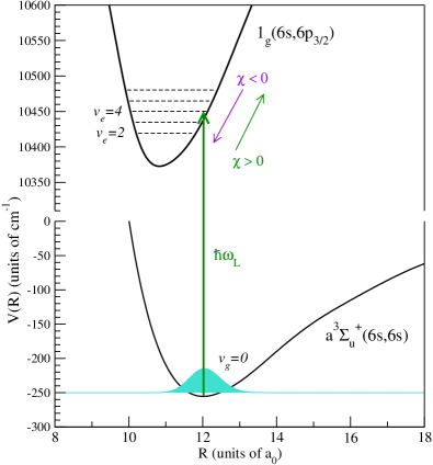
Figure 1: (Color online) $a^{3}\Sigma_{u}^{+}(6s,6s)$ and $1_{g}(6s,6p_{3/2})$ electronic potentials of Cs₂, coupled by a chirped laser pulse with central energy $\hbar\omega_{L}=$ 10695 cm^-1. The initial state of the process is the vibrational wavefunction with $v_{g}=0$ of the $a^{3}\Sigma_{u}^{+}(6s,6s)$ electronic state. The pulse excites several vibrational levels $v_{e}$ in the $1_{g}(6s,6p_{3/2})$ electronic potential. The energy origin is taken to be the dissociation limit $E_{6s+6s}=0$ of the $a^{3}\Sigma_{u}^{+}(6s,6s)$ potential.

We will take as examples transitions implying the electronic states $a^{3}\Sigma_{u}^{+}(6s,6s)$, $1_{g}(6s,6p_{3/2})$, and $0^{-}_{g}(6s,6p_{3/2})$ of the Cs₂ molecule. Sec. V.1 contains a paradigmatic example of two electronic states coupled by a chirped laser pulse which transfers population from the ground electronic state to several vibrational levels of the excited state. We will show that, depending on the quantum preparation, the entanglement dynamics is significantly different. Sec. V.2 shows an example in which three electronic states are populated by a sequence of two chirped laser pulses. The vibrational wave packets excited in each electronic potential are much more complex, having various localizations and intricate vibrational motions.

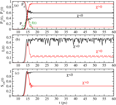
Figure 2: (Color online) Control of the electronic-nuclear entanglement dynamics by the sign of the chirp rate $\chi$, for a coupling $W_{L}=26.34$ cm^-1 between the electronic states $g=a^{3}\Sigma_{u}^{+}$ and $e=1_{g}$ of Cs₂ (Fig. 1). (a) Time evolution of the populations $P_{g}(t)$ and $P_{e}(t)$ for positive and negative chirp. The Gaussian pulse envelope $f(t)$, centered at $t_{P}=15$ ps and with temporal width $\tau_{C}=2.1$ ps, is represented with dashed line. (b) Time evolution of the linear entropy $L(t)$ for positive and negative chirp. (c) Time evolution of the von Neumann entropy $S_{vN}(t)$ for positive and negative chirp.

V.1 Controlling the electronic-nuclear entanglement dynamics in a molecule by populating two electronic states with a chirped laser pulse.

We consider the Cs₂ molecule in which the electronic channels $g=a^{3}\Sigma_{u}^{+}(6s,6s)$ and $e=1_{g}(6s,6p_{3/2})$ are coupled by a chirped laser pulse (Fig. 1), described by the electric field

$${\cal E}(t)={\cal{E}}_{0}f(t)\cos[\omega_{L}t+\varphi(t)],$$ (58)

with amplitude ${\cal{E}}_{0}$ and Gaussian temporal envelope $f(t)$. A chirped pulse Cao et al. (1998); *cao00 is characterized by several parameters belonging to the spectral and temporal domains, which can be used to control the system evolution Luc-Koenig et al. (2004a, b); Vatasescu (2012). $\omega_{L}/2\pi$ is the central frequency of the pulse, reached at $t=t_{P}$, and $\varphi(t)$ is a phase which is a quadratic function of time, such that the instantaneous frequency $\omega(t)=\omega_{L}+d\varphi/dt$ varies linearly with the chirp rate $\chi$ around the central frequency $\omega_{L}/2\pi$: $\omega(t)=\omega_{L}+\chi(t-t_{P})$. The Gaussian envelope $f(t)=\sqrt{\tau_{L}/\tau_{C}}\exp\{-2\ln 2[(t-t_{P})/\tau_{C}]^{2}\}$ is centered at $t=t_{P}$, having the temporal width $\tau_{C}$. The duration $\tau_{L}$ is the temporal width of the transform limited pulse (before chirping), and characterizes the spectral width of the pulse in the frequency domain: $\delta\omega=4\ln 2/\tau_{L}$. The chirp rate $\chi$ and its sign are essential control parameters. The sign of the chirp determines the sense of sweeping the difference $V_{g}(R)-V_{e}(R)$ between the electronic potentials, by increasing or decreasing the instantaneous frequency of the pulse $\omega(t)$ (see Fig. 1), which leads to the excitation of different vibrational wave packets.

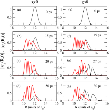
Figure 3: (Color online) Time evolution of the vibrational components $\psi_{g}(R,t)$ (thin line) and $\psi_{e}(R,t)$ (thick line) of the pure entangled state $|\Psi_{el,vib}(t)>$, created by a chirped pulse. (a-d, left column) Time evolution of $|\psi_{g}(R,t)|$, $|\psi_{e}(R,t)|$ for positive chirp, $\chi>0$. (e-h, right column) Time evolution of $|\psi_{g}(R,t)|$, $|\psi_{e}(R,t)|$ for negative chirp, $\chi<0$.

Here we consider a chirped pulse with central energy $\hbar\omega_{L}=$ 10695 cm^-1 which couples the electronic potentials $V_{g}(R)=a^{3}\Sigma_{u}$ and $V_{e}(R)=1_{g}$ of Cs₂ around the internuclear distance $R_{c}\approx 12$ a₀, transferring population from the ground state $v_{g}=0$ of $g=a^{3}\Sigma^{+}_{u}$ to several low vibrational levels $v_{e}$ of the excited state $e=1_{g}$. The process is represented in Fig. 1, the electronic curves being those described in Vatasescu (2009). We suppose a chirped pulse with the envelope $f(t)$ centered at $t_{P}=15$ ps, and temporal width $\tau_{C}=2.1$ ps (represented in Fig. 2(a)), obtained by chirping a transform limited pulse with duration $\tau_{L}=0.3$ ps (spectral width $\delta\omega=49$ cm^-1), using a chirp rate $|\chi|=4.35$ ps^-2. The energy range swept by the chirped pulse around the central frequency $\omega_{L}/2\pi$ is $2\hbar|\chi|\tau_{C}$ Luc-Koenig et al. (2004b), with $\hbar|\chi|=23.11$ cm${}^{-1}/$ps, allowing the excitation of several vibrational levels in the $1_{g}$ potential, where the vibrational level spacing in the excitation range is about 16 cm^-1.

The time-dependent Schrödinger equation describing the dynamics of the vibrational wave packets $\psi_{g,e}(R,t)$ in the electronic channels coupled by the pulse, written using the rotating wave approximation with the frequency $\omega_{L}/2\pi$ Luc-Koenig et al. (2004a); Vatasescu (2012), is

$$i\hbar\frac{\partial}{\partial t}\left(\begin{array}[]{c}\Psi_{e}(R,t)\\ \Psi_{g}(R,t)\end{array}\right)=$$ (61)

$$\left(\begin{array}[]{lc}{\bf\hat{T}}+V^{\prime}_{e}(R)&W_{L}f(t)e^{-i\varphi(t)}\\ W_{L}f(t)e^{i\varphi(t)}&{\bf\hat{T}}+V^{\prime}_{g}(R)\end{array}\right)\left(\begin{array}[]{c}\Psi_{e}(R,t)\\ \Psi_{g}(R,t)\end{array}\right).$$ (66)

In Eq. (61), ${\bf\hat{T}}$ is the kinetic energy operator, and $V^{\prime}_{e}(R)=V_{e}(R)$, $V^{\prime}_{g}(R)=V_{g}(R)+\hbar\omega_{L}$ are the diabatic potentials dressed with the energy $\hbar\omega_{L}$. $W_{L}={\cal{E}}_{0}D_{ge}/2$ is the strength of the laser coupling depending on the laser intensity $I$ (${\cal{E}}_{0}=\sqrt{2I/c\epsilon_{0}}$) and on the transition dipole moment $D_{ge}$ between the electronic surfaces Vatasescu et al. (2001). Here we just use a constant strength coupling $W_{L}$ to explore time evolution under various pulse parameters.

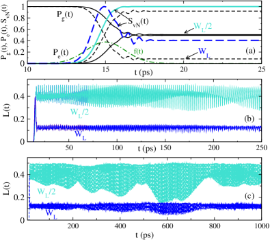
Figure 4: (Color online) Control of electronic-nuclear entanglement dynamics in Cs₂ through the strength $W_{L}$ of the chirped pulse coupling the electronic states $g=a^{3}\Sigma_{u}^{+}$ and $e=1_{g}$ (Fig. 1). Results for $W_{L}=26.34$ cm^-1 and $W_{L}/2$, the last one producing “maximum electronic-nuclear entanglement”. (a) Time evolution of the populations $P_{g}(t)$, $P_{e}(t)$ (full line for $W_{L}/2$, dashed line for $W_{L}$), and of the von Neumann entropy $S_{vN}(t)$ (full line for $W_{L}/2$, dashed line for $W_{L}$) during the pulse. The Gaussian pulse envelope $f(t)$ is represented with dot-dashed line. (b,c) Time evolutions of the linear entropy $L(t)$ after pulse: (b) until 250 ps; (c) until 1000 ps.

The Schrödinger equation (61) is solved numerically by propagating in time the initial wavefunction $\left(\begin{array}[]{c}0\\ \chi_{v_{g}=0}(R)\end{array}\right)$ on a spatial grid with length $L_{R}$, $\chi_{v_{g}=0}(R)$ being the vibrational eigenstate with $v_{g}=0$ in the $a^{3}\Sigma^{+}_{u}$ potential, represented in Fig. 1 and in Figs. 3(a),(e). The time propagation uses the Chebychev expansion of the evolution operator Kosloff (1994, 1996) and the Mapped Sine Grid (MSG) method Luc-Koenig et al. (2004b); Willner et al. (2004) to represent the radial dependence of the wave packets. The populations in each electronic state are calculated from the vibrational wave packets $\Psi_{g,e}(R,t)$ as $P_{g,e}(t)=\int_{0}^{L_{R}}|\Psi_{g,e}(R^{\prime},t)|^{2}dR^{\prime}$, with the total population normalized at 1 on the spatial grid ($P_{g}(t)+P_{e}(t)=1$), and $P_{g}(0)=1$. The von Neumann entropy $S_{vN}(t)$ and the linear entropy $L(t)$ are calculated using the formulas (8) and (11).

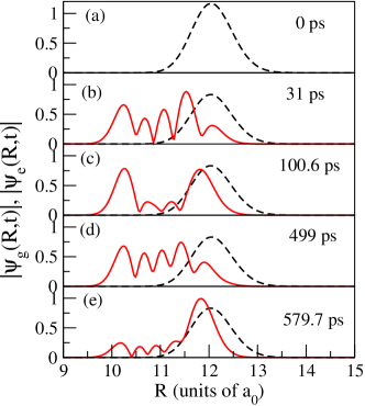
Figure 5: (Color online) Time evolution of the vibrational wave packets $|\psi_{g}(R,t)|$ (dashed line) and $|\psi_{e}(R,t)|$ (thick line) for the case of “maximum entanglement“ achieved by the chirped pulse for a coupling $W_{L}/2$ (Fig. 4).

Figs. 2,3 show results obtained for a positive or a negative chirp rate $\chi$, for the same coupling $W_{L}=26.34$ cm^-1. We see that, by changing the chirp sign, significantly different results are obtained. The pulse with positive chirp $\chi>0$ begins excitation from the lowest $v_{e}$ levels in $1_{g}$, producing an inversion of population between the two electronic channels (Fig. 2(a)) and a “small“ entanglement: the von Neumann entropy after pulse is $S_{vN}(t)=0.4$ (Fig. 2(c)) and the linear entropy oscillates around 0.1 (Fig. 2(b)). The time evolution of the wave packets is shown in Figs. 3(a-d). In the electronic state $g=a^{3}\Sigma^{+}_{u}$ the fundamental vibrational state $v_{g}=0$ (which is the initial state of the process) is the only one populated. The pulse populates the vibrational levels with $v_{e}=2,3$ in the excited state $1_{g}$, separated by $\approx$ 16 cm^-1, which is reflected in the oscillations of about 2 ps in the linear entropy after pulse (Fig. 2(b)). Indeed, in Sec. II.3 we have shown that this is the characteristic time to be expected in the linear entropy evolution in a $2\times 3$ system (one level $v_{g}$ populated in $g$ electronic state, and two levels $v_{e},v^{\prime}_{e}$ in $e$ electronic state), and it coincides with the vibrational period $T_{vib}(v_{e}=3)=2$ ps.

On the contrary, if the chirp is negative, $\chi<0$, the pulse begins by exciting higher vibrational levels in $1_{g}$, and continues with lower vibrational levels. A superposition of vibrational states dominated by $v_{e}=4,5$ is excited in $1_{g}$, and also a superposition of vibrational levels (mainly $v_{g}=3,4,5$) remains populated in $a^{3}\Sigma^{+}_{u}$ (Figs. 3(e-h)). This gives a stronger entanglement: the von Neumann entropy after pulse is close to 1 (Fig. 2(c)). After pulse, the linear entropy (Fig. 2(b)) is a highly oscillating function, whose amplitude varies between 0.33 and 0.5. Since several vibrational states are populated in each electronic potential, there are several characteristic times $T_{osc}$ interwined in $L(t)$ evolution, according to the analysis made in Sec. II.3.

We shall consider now the formation of an entangled state $|\Psi_{el,vib}(t)>$ using the coupling strength $W_{L}$ as a control parameter. Fig. 4 shows results obtained with a chirped pulse having the same parameters as before and positive chirp rate $\chi=4.35$ ps^-2, for the coupling strengths $W_{L}=26.34$ cm^-1 and $W_{L}/2$. The case $W_{L}$ with positive chirp was already analyzed. If the coupling is diminished at $W_{L}/2$, the pulse achieves the equalization of electronic populations $P_{g}(t)=P_{e}(t)=1/2$ (Fig. 4(a)), creating maximum entanglement ($S_{vN}(t)=1$) at the end. The time evolution of the wave packets is shown in Fig. 5, illustrating several instants of the vibrational motion in the excited electronic state. In the electronic state $g=a^{3}\Sigma^{+}_{u}$ only the fundamental vibrational state $v_{g}=0$ is populated, and the vibrational superposition in the excited state $e=1_{g}$ is made mainly by the vibrational levels $v_{e}=3,4$. After pulse, the linear entropy is an oscillating function (Fig. 4(b)) with the main oscillation period equal to $T_{vib}(v_{e}=3)=2$ ps. The long term evolution (until 1000 ps) shows the large amplitude of the linear entropy variations: $L(t)$ oscillates from a maximum of 0.5 to a minimum of 0.15 (Fig. 4(c)). This large difference between $L(t)$ minima and maxima is due to the maximization and minimization of the overlap integral, created by the vibrational motion of the excited wave packet. Figs. 5(d,e) show the vibrational wave packets at $t=499$ ps, when entanglement is maximal ($L(t)\approx 0.5$) and the overlap is minimal, and at $t=579.7$ ps, when the entanglement becomes minimal ($L(t)\approx 0.15$) because the overlap is maximal.

V.2 Entanglement dynamics in a case of three electronic potentials coupled by two chirped laser pulses

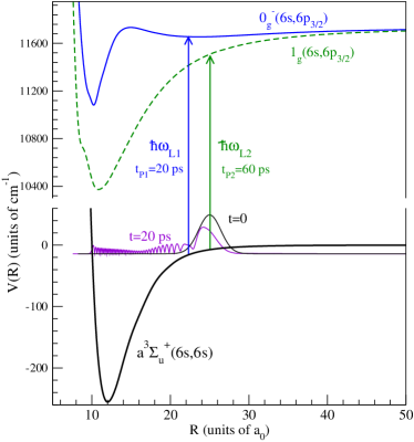
Figure 6: (Color online) $a^{3}\Sigma_{u}^{+}(6s,6s)$, $1_{g}(6s,6p_{3/2})$, and $0_{g}^{-}(6s,6p_{3/2})$ electronic potentials of Cs₂, coupled by two successive chirped laser pulses. The first pulse, with central energy $\hbar\omega_{L1}=11680$ cm^-1, and $t_{P1}=20$ ps, transfers population from $a^{3}\Sigma_{u}^{+}$ to the double well potential $0_{g}^{-}(6s,6p_{3/2})$. The second one, with $\hbar\omega_{L2}=11513$ cm^-1 and centered at $t_{P2}=60$ ps, transfers population from $a^{3}\Sigma_{u}^{+}$ to $1_{g}(6s,6p_{3/2})$. The initial state of the process is a Gaussian wave packet in the $a^{3}\Sigma_{u}^{+}(6s,6s)$ electronic state, represented in the figure. After pulses, all three electronic potentials remain populated. The energy origin is taken to be the dissociation limit $E_{6s+6s}=0$ of the $a^{3}\Sigma_{u}^{+}(6s,6s)$ potential.

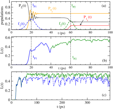
Figure 7: (Color online) Electronic-nuclear entanglement dynamics in the Cs₂ molecule, created by the sequence of two pulses which populate the three electronic potentials represented in Fig. 6. (a) Time evolution of the populations $P_{\Sigma}(t)$, $P_{0_{g}}(t)$, and $P_{1_{g}}(t)$ due to the chirped pulses whose envelopes $f_{1}(t)$ and $f_{2}(t)$ are represented with dashed line. (b) Time evolution of the linear entropy $L(t)$ during the first pulse (after which two electronic states are populated) and the second pulse (which populates also the third one). (c) Long term evolution of the linear entropy $L(t)$. With dashed line is represented the long term evolution of $L(t)$ in the hypothetical case of the first pulse only.

Let us now consider the Cs₂ molecule, in which an entangled state $|\psi_{el,vib}(t)>$ is created by a sequence of two chirped laser pulses, which couple consecutively the electronic state $a^{3}\Sigma_{u}^{+}(6s,6s)$ to $0_{g}^{-}(6s,6p_{3/2})$ and to $1_{g}(6s,6p_{3/2})$. The scheme is shown in Fig. 6. The first pulse couples $a^{3}\Sigma_{u}^{+}$ to $0_{g}^{-}$, leaving both states populated. After the end of the first pulse, the second pulse couples $a^{3}\Sigma_{u}^{+}$ to $1_{g}$. At the end of the sequence, all three electronic states rest populated, in a process which increases progressively the entanglement (from two to three electronic states).

Let us detail the scheme. The initial state of the process, represented in Fig. 6, is a Gaussian wave packet in the electronic $a^{3}\Sigma_{u}^{+}(6s,6s)$ potential, localized around 25 a₀ and simulating a superposition of vibrational states of $a^{3}\Sigma_{u}^{+}(6s,6s)$ centered around the state with $v_{{}_{\Sigma}}=36$, which is bounded by $E_{v_{{}_{\Sigma}}=36}\approx-17$ cm^-1. The two chirped pulses have Gaussian temporal envelopes $f_{1}(t)$ and $f_{2}(t)$, which are centered at $t_{P1}=20$ ps and $t_{P2}=60$ ps, respectively (represented in Fig. 7(a)).

The first chirped pulse, with central energy $\hbar\omega_{L1}=11680$ cm^-1, couples the $a^{3}\Sigma_{u}^{+}$ electronic state to the $0_{g}^{-}(6s,6p_{3/2})$ state. The pulse has the temporal width $\tau_{C1}=7.2$ ps (with $\tau_{L1}=1$ ps) and a positive chirp rate $\chi_{1}=0.379$ ps^-2, such as the energy range resonantly swept around the central frequency is $2\hbar|\chi_{1}|\tau_{C1}\approx 28$ cm^-1. The coupling strength is $W_{L1}=6.6$ cm^-1. The first pulse populates a superposition of vibrational levels in the external well of the $0_{g}^{-}(6s,6p_{3/2})$ potential, exciting also the vibrational level $v_{i}=24$ of the $0_{g}^{-}$ inner well. Fig. 8 shows the vibrational wave packets $a^{3}\Sigma_{u}^{+}$ and $0_{g}^{-}$ populated by the first pulse at t=20 ps. The wave packets evolution during the pulse is obtained by solving numerically a temporal Schrödinger equation similar with Eq. (61). The time evolution of the populations is represented in Fig. 7(a).

The second pulse, with $\hbar\omega_{L2}=11513$ cm^-1 and centered at $t_{P2}=60$ ps, transfers population from $a^{3}\Sigma_{u}^{+}$ to $1_{g}(6s,6p_{3/2})$. The pulse has a coupling strength $W_{L2}=26.3$ cm^-1, temporal width $\tau_{C2}=5$ ps (with $\tau_{L1}=0.5$ ps) and a positive chirp rate $\chi_{2}=1.1$ ps^-2. The energy range resonantly swept around its central frequency $\omega_{L2}/2\pi$ is $2\hbar|\chi_{2}|\tau_{C2}\approx 58.6$ cm^-1, and a superposition of high excited vibrational levels (around the level with $v_{1_{g}}=108$) is populated in the $1_{g}$ electronic potential.

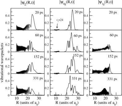
Figure 8: Time evolution of the vibrational wave packets $\psi_{{}_{\Sigma}}(R,t)$, $\psi_{0_{g}}(R,t)$ and $\psi_{1_{g}}(R,t)$ excited by the sequence of two chirped pulses in the electronic potentials $a^{3}\Sigma_{u}^{+}(6s,6s)$, $0_{g}^{-}(6s,6p_{3/2})$, and $1_{g}(6s,6p_{3/2})$, represented in Fig. 6.

Fig. 8 shows the dynamics of the vibrational wave packets in the three electronic potentials. The time evolution of the electronic populations is represented in Fig. 7(a). The chirped Rabi periods characteristic for the action of a chirped pulse Luc-Koenig et al. (2004a) are visible during each pulse.

The linear entropy of entanglement $L(t)$ is calculated using the formula (15), and its time evolution during the pulse sequence is represented in Fig. 7(b). By populating a third electronic state, the second pulse increases the molecular entanglement, as we have shown in Sec. II.2. The long term linear entropy evolution, after the end of the pulse sequence, is shown in Fig. 7(c). In the same figure we have represented $L(t)$ evolution supposing that only the first pulse would act on the molecule, and therefore only two electronic states would be populated. In this case the entanglement dynamics is due to vibronic coherences between only two electronic states, showing large variations between minima and maxima. As we have shown in Sec. III.1, this large amplitude in $L(t)$ variations is an indicator for the strength of the electronic coherence measured by $C_{l_{1}}(\hat{\rho}_{el})$, which is proportional to the overlap $|<\psi_{g}(R,t)|\psi_{e}(R,t)>|$. When three electronic states are populated, entanglement is increased and $L(t)$ variations in time are diminished. This shows a decreasing of the electronic coherence measured by $C_{l_{1}}(\hat{\rho}_{el})$, due to smaller overlaps between the three vibrational wave packets.

Therefore, we have shown examples of a molecule prepared in an electronic-vibrational entangled state by chirped laser pulses which create coherent vibrational wave packets in several electronic potentials. Dephasing and recurrence due to periodic oscillations are specific to wave packets vibrational motion in bound electronic potentials. Electronic-nuclear entanglement oscillations in an isolated molecule so prepared with laser pulses are indicative for phenomena of electronic coherence in the molecular system and periodicity specific to vibrational motions Gruebele and Zewail (1993); *aspuru12; *cina12. Entanglement may be increased by increasing the number of populated electronic states. On the other hand, entanglement oscillations, expressed in the temporal variations of the linear entropy, may be of large amplitude, and can be controlled by quantum preparations.

VI Conclusion

We have derived measures of entanglement and quantum coherence for a molecular system described in a bipartite Hilbert space $\cal{H}$$=$$\cal{H}$_el$\bigotimes$$\cal{H}$_vib of dimension $N_{el}\times N_{v}$, establishing relations between the linear entropy of electronic-vibrational entanglement and quantifiers of quantum coherence in the bipartite molecular system.

For a Hilbert space of dimension $2\times N_{v}$, we have discussed the expressions for the von Neumann and linear entropy of electronic-nuclear entanglement Vatasescu (2013), showing that a remarkable difference between these two measures of entanglement appears when their temporal behaviours in the case of an isolated molecule are considered. In contrast to the von Neumann entropy of entanglement, the linear entropy ”understands” vibrational motion in the electronic potentials as entanglement dynamics. We find linear entropy of entanglement as being a more complex informational quantity, recalling previous assertions about the ”conceptual inadequacy” Brukner and Zeilinger (2001) of the von Neumann entropy in defining the information content of a quantum system. These discussions were accompanied by proposals for a more appropriate measure, which, interestingly, has proven to be essentially the linear entropy Brukner and Zeilinger (1999, 2001); Luo (2006).

We have derived the linear entropy of electronic-vibrational entanglement for a bipartite Hilbert space $\cal{H}$$=$$\cal{H}$_el$\bigotimes$$\cal{H}$_vib with dimension $N_{el}\times N_{v}$, showing its dependence on the vibronic coherences of the molecule, a property that connects this entanglement measure to coherence quantifiers.

Quantum coherence in the bipartite entangled state $\hat{\rho}_{el,vib}(t)$ was characterized employing the resource approach Baumgratz et al. (2014); Girolami (2014), using measures of coherence based on $l_{1}$ norm and Wigner-Yanase skew information. Connections between quantum coherence, quantum uncertainty in energy, and the ”velocity” of $\hat{\rho}_{el,vib}(t)$ evolution Anandan and Aharonov (1990) are outlined in Sec. III.2.

We have employed the skew information as a measure of quantum coherence and quantum uncertainty in the pure entangled state $\hat{\rho}_{el,vib}(t)$ and in the reduced electronic state $\hat{\rho}_{el}$, taking as observables the Hamiltonians $\hat{H}_{mol}$ and $\hat{H}_{el}$. We have derived the Wigner-Yanase skew information in the reduced electronic state $\hat{\rho}_{el}$ for the electronic Hamiltonian $\hat{H}_{el}$, and in the pure entangled state $\hat{\rho}_{el,vib}(t)$ for the observables $\hat{H}_{mol}$ (molecular Hamiltonian) and $\hat{H}_{el}\bigotimes\hat{I}_{v}$ (local observable $\hat{H}_{el}$), for a bipartite Hilbert space of dimension $N_{el}\times N_{v}$. We have shown that linear entropy of entanglement is connected to the skew information ${\cal I_{S}}(\hat{\rho}_{el,vib},\hat{H}_{el}\bigotimes\hat{I}_{v})$ and ${\cal I_{S}}(\hat{\rho}_{el},\hat{H}_{el})$, related to the measurement of the local observable $\hat{H}_{el}$ in the correlated quantum systems (el$\bigotimes$vib).

The characteristic times of entanglement dynamics due to vibrational motion in the electronic potentials are analyzed in Sec. II.3. In the last part of this paper, Sec. V.1, we show examples of these entanglement oscillations for the $Cs_{2}$ molecule prepared in an electronic-vibrational entangled state by chirped laser pulses which create coherent vibrational wave packets in several electronic potentials. We have shown the control of entanglement dynamics by using chirped laser pulses, whose parameters can be chosen to create specific quantum preparations and significant changes in entanglement dynamics.

We hope that the present work will contribute to the ample research program intended to enlighten our understanding of molecular phenomena by using quantum information concepts.